GDI: Rethinking What Makes Reinforcement Learning Different from Supervised Learning

Abstract

Deep Q Network (DQN) firstly kicked the door of deep reinforcement learning (DRL) via combining deep learning (DL) with reinforcement learning (RL), which has noticed that the distribution of the acquired data would change during the training process. DQN found this property might cause instability for training, so it proposed effective methods to handle the downside of the property. Instead of focusing on the unfavorable aspects, we find it critical for RL to ease the gap between the estimated data distribution and the ground truth data distribution while supervised learning (SL) fails to do so. From this new perspective, we extend the basic paradigm of RL called the Generalized Policy Iteration (GPI) into a more generalized version, which is called the Generalized Data Distribution Iteration (GDI). We see massive RL algorithms and techniques can be unified into the GDI paradigm, which can be considered as one of the special cases of GDI. We provide theoretical proof of why GDI is better than GPI and how it works. Several practical algorithms based on GDI have been proposed to verify its effectiveness and extensiveness. Empirical experiments prove our state-of-the-art (SOTA) performance on Arcade Learning Environment (ALE), wherein our algorithm has achieved 9620.98% mean human normalized score (HNS), 1146.39% median HNS and 22 human world record breakthroughs (HWRB) using only 200M training frames. Our work aims to lead the RL research to step into the journey of conquering the human world records and seek real superhuman agents on both performance and efficiency.

1 Introduction

Machine learning (ML) can be defined as improving some measure performance P at some task T according to the acquired data or experience E (Mitchell, others, 1997). As one of the three main components of ML (Mitchell, others, 1997), the training experiences matter in ML, which can be reflected from many aspects. For example, three major ML paradigms can be distinguished from the perspective of the different training experiences. Supervised learning (SL) is learning from a training set of labeled experiences provided by a knowledgable external supervisor (Sutton, Barto, 2018). Unsupervised learning (UL) is typically about seeking structure hidden in collections of unlabeled experiences (Sutton, Barto, 2018). Unlike UL or SL, reinforcement learning (RL) focuses on the problem that agents learn from experiences gained through trial-and-error interactions with a dynamic environment (Kaelbling et al., 1996). As (Mitchell, others, 1997) said, there is no free lunch in the ML problem - no way to generalize beyond the specific training examples. The performance can only be improved through learning from the acquired experiences in ML problems (Mitchell, others, 1997). All of them have revealed the importance of the training experiences and thus the selection of the training distribution appears to be a fundamental problem in ML.

Recalling these three paradigms, SL and RL receive explicit learning signals from data. In SL, there is no way to make up the gap between the distribution estimated by the collected data and the ground truth without any domain knowledge unless collecting more data. Researchers have found RL explicitly and naturally transforming the training distribution (Mnih et al., 2015), which makes RL distinguished from SL. In the recent RL advances, many researchers (Mnih et al., 2015) have realized that RL agents hold the property of changing the data distribution and massive works have revealed the unfavorable aspect of the property. Among those algorithms, DQN (Mnih et al., 2015) firstly noticed the unique property of RL and considered it as one of the reasons for the training instability of DRL. After that, massive methods like replay buffer (Mnih et al., 2015), periodically updated target (Mnih et al., 2015) and importance sampling (Espeholt et al., 2018) have been proposed to mitigate the impact of the data distribution shift. However, after rethinking this property, we wonder whether changing the data distribution always brings unfavorable nature. What if we can control it? More precisely, what if we can control the ability to select superior data distribution for training automatically? Prior works in ML have revealed the great potential of this property. As (Cohn et al., 1996) put it, when training examples are appropriately selected, the data requirements for some problems decrease drastically, and some NP-complete learning problems become polynomial in computation time (Angluin, 1988; Baum, 1991), which means that carefully selecting good training data benefits learning efficiency. Inspired by this perspective, instead of discussing how to ease the disadvantages caused by the change of data distribution like other prior works of RL, in this paper, we rethink the property distinguishing RL from SL and explore more effective aspects of it. One of the fundamental reasons RL holds the ability to change the data distribution is the change of behavior policies, which directly interact with the dynamic environments to obtain training data (Mnih et al., 2015). Therefore, the training experiences can be controlled by adjusting the behavior policies, which makes behavior selection the bridge between RL agents and training examples.

In the RL problem, the agent has to exploit what it already knows to obtain the reward, but it also has to explore to make better action selections in the future, which is called the exploration and exploitation dilemma (Sutton, Barto, 2018). Therefore, diversity is one of the main factors that should be considered while selecting the training examples. In the recent advances of RL, some works have also noticed the importance of the diversity of training experiences (Badia et al., 2020a, b; Parker-Holder et al., 2020; Niu et al., 2011; Li et al., 2019; Eysenbach et al., 2018), most of which have obtained diverse data via enriching the policy diversity. Among those algorithms, DIAYN (Eysenbach et al., 2018) focused entirely on the diversity of policy via learning skills without a reward function, which has revealed the effect of policy diversity but ignored its relationship with the RL objective. DvD (Parker-Holder et al., 2020) introduced a diversity-based regularizer into the RL objective to obtain more diverse data, which changed the optimal solution of the environment (Sutton, Barto, 2018). Besides, training a population of agents to gather more diverse experiences seems to be a promising approach. Agent57 (Badia et al., 2020a) and NGU (Badia et al., 2020b) trained a family of policies with different degrees of exploratory behaviors using a shared network architecture. Both of them have obtained SOTA performance at the cost of increasing the uncertainty of environmental transition, which leads to extremely low learning efficiency. Through those successes, it is evident that the diversity of the training data benefit the RL training. However, why does it perform better and whether more diverse data always benefit RL training? In other words, we have to explore the following question:

Does diverse data always benefit effective learning?

To investigate this problem, we seek inspiration from the natural biological processes. In nature, the population evolves typically faster than individuals because the diversity of the populations boosts more beneficial mutations which provide more possibility for acquiring more adaptive direction of evolution (Pennisi, 2016). Furthermore, beneficial mutations rapidly spread among the population, thus enhancing population adaptability (Pennisi, 2016). Therefore, an appropriate diversity brings high-value individuals, and active learning among the population promotes its prosperity. From this perspective, the RL agents have to pay more attention to experiences worthy of learning from. DisCor (Kumar et al., 2020), which re-weighted the existing data buffer by the distribution that explicitly optimizes for corrective feedback, has also noticed the fact that the choice of the sampling distribution is of crucial importance for the stability and efficiency of approximation dynamic programming algorithms. Unfortunately, DisCor only changes the existing data distribution instead of directly controlling the source of the training experiences, which may be more important and also more complex. In conclusion, it seems that both expanding the capacity of policy space for behaviors and selecting suitable behavior policies from a diverse behavior population matter for efficient learning. This new perspective motivates us to investigate another critical problem:

How to select superior behaviors from the behavior policy space?

To address those problems, we proposed a novel RL paradigm called Generalized Data Distribution Iteration (GDI), which consists of two major process, the policy iteration operator $\mathcal{T}$ and the data distribution iteration operator $\mathcal{E}$. Specifically, behaviors will be sampled from a policy space according to a selective distribution, which will be iteratively optimized through the operator $\mathcal{E}$. Simultaneously, elite training data will be used for policy iteration via the operator $\mathcal{T}$. More details about our methodology can see Sec. 3.

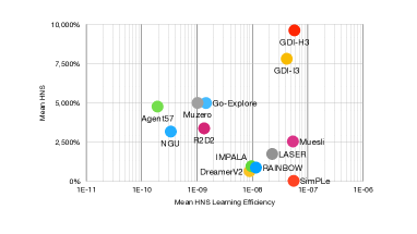
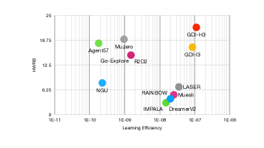
Figure 1: Performance of SOTA algorithms of Atari 57 games on mean HNS(%) with corresponding learning efficiency and human world record breakthrough with corresponding game time. Details on those evaluation criteria can see App. H.

In conclusion, the main contributions of our work are:

• A Novel RL Paradigm: Rethinking the difference between RL and SL, we discover RL can ease the gap between the sampled data distribution and the ground truth data distribution via adjusting the behavior policies. Based on the perspective, we extend GPI into GDI, a more general version containing a data optimization process. This novel perspective allows us to unify massive RL algorithms, and various improvements can be considered a special case of data distribution optimization, detailed in Sec. 3.

• Theoretical Proof of GDI: We provide sufficient theoretical proof of GDI. The effectiveness of the data distribution optimization of GDI has been proved on both first-order optimization and second-order optimization, and the guarantee of monotonic improvement induced by the data distribution optimization operator $\mathcal{E}$ has also been proved. More details can see Sec. 3 and App. E.

• A General Practical Framework of GDI: Based on GDI, we propose a general practical framework, wherein behavior policy belongs to a soft $\epsilon$-greedy space which unifies $\epsilon$-greedy policies (Watkins, 1989) and Boltzmann policies (Wiering, 1999). As a practical framework of GDI, a self-adaptable meta-controller is proposed to optimize the distribution of the behavior policies. More implementation details can see App. F and App. G.

• The State-Of-The-Art Performance: From Figs. 1, our approach has achieved 9620.98% mean HNS and 1146.39% median HNS, which achieves new SOTA. More importantly, our learning efficiency has approached the human level as achieving the SOTA performance within less than 1.5 months of game time. We have also illustrated the RL Benchmark on HNS in App. D.1 and recorded their scores in App. J.5.

• Human World Records Breakthrough: As our algorithms have achieved SOTA on mean HNS, median HNS and learning efficiency, we aim to lead RL research on ALE to step into a new era of conquering human world records and seeking the real superhuman agents. Therefore, we propose several novel evaluation criteria and an open challenge on the Atari benchmark based on the human world records. From Figs. 1, our method has surpassed 22 human world records, which has also surpassed all previous algorithms. We have also illustrated the RL Benchmark on human world records normalized scores (HWRNS), SABER (Toromanoff et al., 2019), HWRB in App. D.2, D.3 and D.4, respectively. Relevant scores are recorded in App. J.6 and App. J.7.

2 Preliminaries

The RL problem can be formulated as a Markov Decision Process (Howard, 1960, MDP) defined by $\left(\mathcal{S},\mathcal{A},p,r,\gamma,\rho_{0}\right)$. Considering a discounted episodic MDP, the initial state $s_{0}$ is sampled from the initial distribution $\rho_{0}(s):\mathcal{S}\rightarrow\Delta(\mathcal{S})$, where we use $\Delta$ to represent the probability simplex. At each time $t$, the agent chooses an action $a_{t}\in\mathcal{A}$ according to the policy $\pi(a_{t}|s_{t}):\mathcal{S}\rightarrow\Delta(\mathcal{A})$ at state $s_{t}\in\mathcal{S}$. The environment receives $a_{t}$, produces the reward $r_{t}\sim r(s,a):\mathcal{S}\times\mathcal{A}\rightarrow\mathbf{R}$ and transfers to the next state $s_{t+1}$ according to the transition distribution $p\left(s^{\prime}\mid s,a\right):\mathcal{S}\times\mathcal{A}\rightarrow\Delta(\mathcal{S})$. The process continues until the agent reaches a terminal state or a maximum time step. Define the discounted state visitation distribution as $d_{\rho_{0}}^{\pi}(s)=(1-\gamma)\textbf{E}_{s_{0}\sim\rho_{0}}\left[\sum_{t=0}^{\infty}\gamma^{t}\textbf{P}(s_{t}=s|s_{0})\right]$. The goal of reinforcement learning is to find the optimal policy $\pi^{*}$ that maximizes the expected sum of discounted rewards, denoted by $\mathcal{J}$ (Sutton, Barto, 2018):

$$\pi^{*}=\underset{\pi}{\operatorname{argmax}}\mathcal{J}_{\pi}=\underset{\pi}{\operatorname{argmax}}\textbf{E}_{s_{t}\sim d_{\rho_{0}}^{\pi}}\textbf{E}_{\pi}\left[G_{t}|s_{t}\right]=\underset{\pi}{\operatorname{argmax}}\textbf{E}_{s_{t}\sim d_{\rho_{0}}^{\pi}}\textbf{E}_{\pi}\left[\sum_{k=0}^{\infty}\gamma^{k}r_{t+k}|s_{t}\right]$$ (1)

where $\gamma\in(0,1)$ is the discount factor.

RL algorithms can be divided into off-policy manners (Mnih et al., 2015, 2016; Haarnoja et al., 2018; Espeholt et al., 2018) and on-policy manners (Schulman et al., 2017b). Off-policy algorithms select actions according to a behavior policy $\mu$ that can be different from the learning policy $\pi$. On-policy algorithms evaluate and improve the learning policy through data sampled from the same policy. RL algorithms can also be divided into value-based methods (Mnih et al., 2015; Van Hasselt et al., 2016; Wang et al., 2016; Hessel et al., 2017; Horgan et al., 2018) and policy-based methods (Schulman et al., 2017b; Mnih et al., 2016; Espeholt et al., 2018; Schmitt et al., 2020). In the value-based methods, agents learn the policy indirectly, where the policy is defined by consulting the learned value function, like $\epsilon$-greedy, and the value function is learned by a typical GPI. In the policy-based methods, agents learn the policy directly, where the correctness of the gradient direction is guaranteed by the policy gradient theorem (Sutton, Barto, 2018), and the convergence of the policy gradient methods is also guaranteed (Agarwal et al., 2019). More background on RL can see App. B.

3 Methodology

3.1 Generalized Data Distribution Iteration

Let’s abstract our notations first, which is also summarized in App. A.

Define $\Lambda$ to be an index set, $\Lambda\subseteq\textbf{R}^{k}$. $\lambda\in\Lambda$ is an index in $\Lambda$. $(\Lambda,\mathcal{B}|_{\Lambda},\mathcal{P}_{\Lambda})$ is a probability space, where $\mathcal{B}|_{\Lambda}$ is a Borel $\sigma$-algebra restricted to $\Lambda$. Under the setting of meta-RL, $\Lambda$ can be regarded as the set of all possible meta information. Under the setting of population-based training (PBT) (Jaderberg et al., 2017), $\Lambda$ can be regarded as the set of the whole population.

Define $\Theta$ to be a set of all possible values of parameters. $\theta\in\Theta$ is some specific value of parameters. For each index $\lambda$, there exists a specific mapping between each parameter of $\theta$ and $\lambda$, denoted as $\theta_{\lambda}$, to indicate the parameters in $\theta$ corresponding to $\lambda$. Under the setting of linear regression $y=w\cdot x$, $\Theta=\{w\in R^{n}\}$ and $\theta=w$. If $\lambda$ represents using only the first half features to make regression, assume $w=(w_{1},w_{2})$, then $\theta_{\lambda}=w_{1}$. Under the setting of RL, $\theta_{\lambda}$ defines a parameterized policy indexed by $\lambda$, denoted as $\pi_{\theta_{\lambda}}$.

Define $\mathcal{D}\overset{def}{=}\{d^{\pi}_{\rho_{0}}|\ \pi\in{\Delta(\mathcal{A})}^{\mathcal{S}},\rho_{0}\in\Delta(\mathcal{S})\}$ to be the set of all states visitation distributions. For the parameterized policies, denote $\mathcal{D}_{\Lambda,\Theta,\rho_{0}}\overset{def}{=}\{d^{\pi_{\theta_{\lambda}}}_{\rho_{0}}|\ \theta\in\Theta,\lambda\in\Lambda\}$. Note that $(\Lambda,\mathcal{B}|_{\Lambda},\mathcal{P}_{\Lambda})$ is a probability space on $\Lambda$, which induces a probability space on $\mathcal{D}_{\Theta,\Lambda,\rho_{0}}$, with the probability measure given by $\mathcal{P}_{\mathcal{D}}(\mathcal{D}_{\Lambda_{0},\Theta,\rho_{0}})=\mathcal{P}_{\Lambda}(\Lambda_{0}),\ \forall\Lambda_{0}\in\mathcal{B}|_{\Lambda}$.

We use $x$ to represent one sample, which contains all necessary information for learning. For DQN, $x=(s_{t},a_{t},r_{t},s_{t+1})$. For R2D2, $x=(s_{t},a_{t},r_{t},\dots,s_{t+N},a_{t+N},r_{t+N},s_{t+N+1})$. For IMPALA, $x$ also contains the distribution of the behavior policy. The content of $x$ depends on the algorithm, but it’s sufficient for learning. We use $\mathcal{X}$ to represent the set of samples. At training stage $t$, given the parameter $\theta=\theta^{(t)}$, the distribution of the index set $\mathcal{P}_{\Lambda}=\mathcal{P}^{(t)}_{\Lambda}$ and the distribution of the initial state $\rho_{0}$, we denote the set of samples as

$$\mathcal{X}_{\rho_{0}}^{(t)}\overset{def}{=}\bigcup_{d_{\rho_{0}}^{\pi}\sim\mathcal{P}_{\mathcal{D}}^{(t)}}\{x|x\sim d_{\rho_{0}}^{\pi}\}=\bigcup_{\lambda\sim\mathcal{P}_{\Lambda}^{(t)}}\{x|x\sim d_{\rho_{0}}^{\pi_{\theta}},\theta={\theta^{(t)}_{\lambda}}\}\triangleq\bigcup_{\lambda\sim\mathcal{P}_{\Lambda}^{(t)}}\mathcal{X}^{(t)}_{\rho_{0},\lambda}.$$

Now we introduce our main algorithm:

Algorithm 1 Generalized Data Distribution Iteration (GDI).

  Initialize $\Lambda$, $\Theta$, $\mathcal{P}_{\Lambda}^{(0)}$, $\theta^{(0)}$.

  for $t=0,1,2,\dots$ do

     Sample $\{\mathcal{X}^{(t)}_{\rho_{0},\lambda}\}_{\lambda\sim\mathcal{P}^{(t)}_{\Lambda}}$.

     $\theta^{(t+1)}=\mathcal{T}(\theta^{(t)},\{\mathcal{X}^{(t)}_{\rho_{0},\lambda}\}_{\lambda\sim\mathcal{P}^{(t)}_{\Lambda}})$.

     $\mathcal{P}_{\Lambda}^{(t+1)}=\mathcal{E}(\mathcal{P}_{\Lambda}^{(t)},\{\mathcal{X}^{(t)}_{\rho_{0},\lambda}\}_{\lambda\sim\mathcal{P}^{(t)}_{\Lambda}})$.

  end for

$\mathcal{T}$ defined as $\theta^{(t+1)}=\mathcal{T}(\theta^{(t)},\{\mathcal{X}^{(t)}_{\rho_{0},\lambda}\}_{\lambda\sim\mathcal{P}^{(t)}_{\Lambda}})$ is a typical optimization operator of RL algorithms, which utilizes the collected samples to update the parameters for maximizing some function $L_{\mathcal{T}}$. For instance, $L_{\mathcal{T}}$ may contain the policy gradient and the state value evaluation for the policy-based methods, may contain generalized policy iteration for the value-based methods, may also contain some auxiliary tasks or intrinsic rewards for special designed methods.

$\mathcal{E}$ defined as $\mathcal{P}_{\Lambda}^{(t+1)}=\mathcal{E}(\mathcal{P}_{\Lambda}^{(t)},\{\mathcal{X}^{(t)}_{\rho_{0},\lambda}\}_{\lambda\sim\mathcal{P}^{(t)}_{\Lambda}})$ is a data distribution optimization operator. It uses the samples $\{\mathcal{X}^{(t)}_{\rho_{0},\lambda}\}_{\lambda\sim\mathcal{P}^{(t)}_{\Lambda}}$ to maximize some function $L_{\mathcal{E}}$, namely,

$$\mathcal{P}_{\Lambda}^{(t+1)}=\operatorname*{arg\,max}_{\mathcal{P}_{\Lambda}}L_{\mathcal{E}}(\{\mathcal{X}^{(t)}_{\rho_{0},\lambda}\}_{\lambda\sim\mathcal{P}_{\Lambda}}).$$

When $\mathcal{P}_{\Lambda}$ is parameterized, we abuse the notation and use $\mathcal{P}_{\Lambda}$ to represent the parameter of $\mathcal{P}_{\Lambda}$. If $\mathcal{E}$ is a first order optimization operator, then we can write $\mathcal{E}$ explicitly as

$$\mathcal{P}_{\Lambda}^{(t+1)}=\mathcal{P}_{\Lambda}^{(t)}+\eta\nabla_{\mathcal{P}_{\Lambda}^{(t)}}L_{\mathcal{E}}(\{\mathcal{X}^{(t)}_{\rho_{0},\lambda}\}_{\lambda\sim\mathcal{P}^{(t)}_{\Lambda}}).$$

If $\mathcal{E}$ is a second order optimization operator, like natural gradient, we can write $\mathcal{E}$ formally as

$$\mathcal{P}_{\Lambda}^{(t+1)}=\mathcal{P}_{\Lambda}^{(t)}+\eta\textbf{F}(\mathcal{P}_{\Lambda}^{(t)})^{\dagger}\nabla_{\mathcal{P}_{\Lambda}^{(t)}}L_{\mathcal{E}}(\{\mathcal{X}^{(t)}_{\rho_{0},\lambda}\}_{\lambda\sim\mathcal{P}^{(t)}_{\Lambda}}),$$

$$\textbf{F}(\mathcal{P}_{\Lambda}^{(t)})=\left[\nabla_{\mathcal{P}_{\Lambda}^{(t)}}\log\mathcal{P}_{\Lambda}^{(t)}\right]\cdot\left[\nabla_{\mathcal{P}_{\Lambda}^{(t)}}\log\mathcal{P}_{\Lambda}^{(t)}\right]^{\top},$$

where $\dagger$ denotes the Moore-Penrose pseudoinverse of the matrix.

3.2 Systematization of GDI

We can further divide all algorithms into two categories, GDI-Iⁿ and GDI-Hⁿ. $n$ represents the degree of freedom of $\Lambda$. I represents Isomorphism. We say one algorithm belongs to GDI-Iⁿ, if $\theta=\theta_{\lambda},\,\forall\lambda\in\Lambda$. H represents Heterogeneous. We say one algorithm belongs to GDI-Hⁿ, if $\theta_{\lambda_{1}}\neq\theta_{\lambda_{2}},\,\exists\lambda_{1},\lambda_{2}\in\Lambda$. We say one algorithm is "w/o $\mathcal{E}$" if it doesn’t have the operator $\mathcal{E}$, in another word, its $\mathcal{E}$ is an identical mapping.

Now we discuss the connections between GDI and some algorithms.

For DQN, RAINBOW, PPO and IMPALA, they are in GDI-I⁰ w/o $\mathcal{E}$. Let $|\Lambda|=1$, WLOG, assume $\Lambda=\{\lambda_{0}\}$. The probability measure $\mathcal{P}_{\Lambda}$ collapses to $\mathcal{P}_{\Lambda}(\lambda_{0})=1$. $\Theta=\{\theta_{\lambda_{0}}\}$. $\mathcal{E}$ is an identical mapping of $\mathcal{P}_{\Lambda}^{(t)}$. $\mathcal{T}$ is the first order operator that optimizes the loss functions, respectively.

For Ape-X and R2D2, they are in GDI-I¹ w/o $\mathcal{E}$. Let $\Lambda=\{\epsilon_{l}|\ l=1,\dots,256\}$. $\mathcal{P}_{\Lambda}$ is uniform, $\mathcal{P}_{\Lambda}(\epsilon_{l})=|\Lambda|^{-1}$. Since all actors and the learner share parameters, we have $\theta_{\epsilon_{1}}=\theta_{\epsilon_{2}}$ for $\forall\epsilon_{1},\epsilon_{2}\in\Lambda$, hence $\Theta=\bigcup_{\epsilon\in\Lambda}\{\theta_{\epsilon}\}=\{\theta_{\epsilon_{l}}\},\ \forall\ l=1,\dots,256$. $\mathcal{E}$ is an identical mapping, because $\mathcal{P}_{\Lambda}^{(t)}$ is always a uniform distribution. $\mathcal{T}$ is the first order operator that optimizes the loss functions.

For LASER, it’s in GDI-H¹ w/o $\mathcal{E}$. Let $\Lambda=\{i|\ i=1,\dots,K\}$ to be the number of learners. $\mathcal{P}_{\Lambda}$ is uniform, $\mathcal{P}_{\Lambda}(i)=|\Lambda|^{-1}$. Since different learners don’t share parameters, $\theta_{i_{1}}\cap\theta_{i_{2}}=\emptyset$ for $\forall i_{1},i_{2}\in\Lambda$, hence $\Theta=\bigcup_{i\in\Lambda}\{\theta_{i}\}$. $\mathcal{E}$ is an identical mapping. $\mathcal{T}$ can be formulated as a union of $\theta^{(t+1)}_{i}=\mathcal{T}_{i}(\theta^{(t)}_{i},\{\mathcal{X}^{(t)}_{\rho_{0},\lambda}\}_{\lambda\sim\mathcal{P}^{(t)}_{\Lambda}})$, which represents optimizing $\theta_{i}$ of $i$th learner with shared samples from other learners.

For PBT, it’s in GDI-Hⁿ⁺¹, where $n$ is the number of searched hyperparameters. Let $\Lambda=\{h\}\times\{i|i=1,\dots,K\}$, where $h$ represents the hyperparameters being searched and $K$ is the population size. $\Theta=\bigcup_{i=1,\dots,K}\{\theta_{i,h}\}$, where $\theta_{i,h_{1}}=\theta_{i,h_{2}}$ for $\forall(h_{1},i),(h_{2},i)\in\Lambda$. $\mathcal{E}$ is the meta-controller that adjusts $h$ for each $i$, which can be formally written as $\mathcal{P}_{\Lambda}^{(t+1)}(\cdot,i)=\mathcal{E}_{i}(\mathcal{P}_{\Lambda}^{(t)}(\cdot,i),\{\mathcal{X}^{(t)}_{\rho_{0},(h,i)}\}_{h\sim\mathcal{P}^{(t)}_{\Lambda}(\cdot,i)})$, which optimizes $\mathcal{P}_{\Lambda}$ according to the performance of all agents in the population. $\mathcal{T}$ can also be formulated as a union of $\mathcal{T}_{i}$, but is $\theta^{(t+1)}_{i}=\mathcal{T}_{i}(\theta^{(t)}_{i},\{\mathcal{X}^{(t)}_{\rho_{0},(h,i)}\}_{h\sim\mathcal{P}^{(t)}_{\Lambda}(\cdot,i)})$, which represents optimizing the $i$th agent with only samples from the $i$th agent.

For NGU and Agent57, it’s in GDI-I². Let $\Lambda=\{\beta_{i}|i=1,\dots,m\}\times\{\gamma_{j}|j=1,\dots,n\}$, where $\beta$ is the weight of the intrinsic value function and $\gamma$ is the discount factor. Since all actors and the learner share variables, $\Theta=\bigcup_{(\beta,\gamma)\in\Lambda}\{\theta_{(\beta,\gamma)}\}=\{\theta_{(\beta,\gamma)}\}$ for $\forall(\beta,\gamma)\in\Lambda$. $\mathcal{E}$ is an optimization operator of a multi-arm bandit controller with UCB, which aims to maximize the expected cumulative rewards by adjusting $\mathcal{P}_{\Lambda}$. Different from above, $\mathcal{T}$ is identical to our general definition $\theta^{(t+1)}=\mathcal{T}(\theta^{(t)},\{\mathcal{X}^{(t)}_{\rho_{0},\lambda}\}_{\lambda\sim\mathcal{P}^{(t)}_{\Lambda}})$, which utilizes samples from different $\lambda$s to update the shared $\theta$.

For Go-Explore, it’s in GDI-H¹. Let $\Lambda=\{\tau\}$, where $\tau$ represents the stopping time of switching between robustification and exploration. $\Theta=\{\theta_{r}\}\cup\{\theta_{e}\}$, where $\theta_{r}$ is the robustification model and $\theta_{e}$ is the exploration model. $\mathcal{E}$ is a search-based controller, which defines the next $\mathcal{P}_{\Lambda}$ for a better exploration. $\mathcal{T}$ can be decomposed into $(\mathcal{T}_{r},\mathcal{T}_{e})$.

3.3 Monotonic Data Distribution Optimization

We see massive algorithms can be formulated as a special case of GDI. For the algorithms without a meta-controller, whose data distribution optimization operator $\mathcal{E}$ is trivially an identical mapping, the guarantee that the learned policy could converge to the optimal policy has been wildly studied, for instance, GPI in (Sutton, Barto, 2018) and policy gradient in (Agarwal et al., 2019). But for the algorithms with a meta-controller, whose data distribution optimization operator $\mathcal{E}$ is non-identical, though most algorithms in this class show superior performance, it still lacks a general study on why the data distribution optimization operator $\mathcal{E}$ helps. In this section, with a few assumptions, we show that given the same optimization operator $\mathcal{T}$, a GDI with a non-identical data distribution optimization operator $\mathcal{E}$ is always superior to a GDI w/o $\mathcal{E}$.

For brevity, we denote the expectation of $L_{\mathcal{E}},L_{\mathcal{T}}$ for each $\lambda\in\Lambda$ as $\mathcal{L}_{\mathcal{E}}(\lambda,\theta_{\lambda})=\textbf{E}_{x\sim\pi_{\theta_{\lambda}}}[L_{\mathcal{E}}(\{\mathcal{X}_{\rho_{0},\lambda}\})],\ \mathcal{L}_{\mathcal{T}}(\lambda,\theta_{\lambda})=\textbf{E}_{x\sim\pi_{\theta_{\lambda}}}[L_{\mathcal{T}}(\{\mathcal{X}_{\rho_{0},\lambda}\})],$ and denote the expectation of $L_{\mathcal{E}},L_{\mathcal{T}}$ for any $\mathcal{P}_{\Lambda}$ as $\mathcal{L}_{\mathcal{E}}(\mathcal{P}_{\Lambda},\theta)=\textbf{E}_{\lambda\sim\mathcal{P}_{\Lambda}}[\mathcal{L}_{\mathcal{E}}(\lambda,\theta_{\lambda})],\ \mathcal{L}_{\mathcal{T}}(\mathcal{P}_{\Lambda},\theta)=\textbf{E}_{\lambda\sim\mathcal{P}_{\Lambda}}[\mathcal{L}_{\mathcal{T}}(\lambda,\theta_{\lambda})].$

Assumption 1 (Uniform Continuous Assumption).

For $\forall\epsilon>0,\ \forall s\in\mathcal{S},\ \exists\,\delta>0,\ s.t.|V^{\pi_{1}}(s)-V^{\pi_{2}}(s)|<\epsilon,\ \forall\,d_{\pi}(\pi_{1},\pi_{2})<\delta$, where $d_{\pi}$ is a metric on ${\Delta(\mathcal{A})}^{\mathcal{S}}$. If $\pi$ is parameterized by $\theta$, then for $\forall\epsilon>0,\ \forall s\in\mathcal{S},\ \exists\,\delta>0,\ s.t.|V^{\pi_{\theta_{1}}}(s)-V^{\pi_{\theta_{2}}}(s)|<\epsilon,\ \forall\,||\theta_{1}-\theta_{2}||<\delta$.

Remark.

(Dadashi et al., 2019) shows $V^{\pi}$ is infinitely differentiable everywhere on $\Delta(\mathcal{A})^{\mathcal{S}}$ if $|\mathcal{S}|<\infty,|\mathcal{A}|<\infty$. (Agarwal et al., 2019) shows $V^{\pi}$ is $\beta$-smooth, namely bounded second order derivative, for direct parameterization. If $\Delta(\mathcal{A})^{\mathcal{S}}$ is compact, continuity implies uniform continuity.

Assumption 2 (Formulation of $\mathcal{E}$ Assumption).

Assume $\mathcal{P}_{\Lambda}^{(t+1)}=\mathcal{E}(\mathcal{P}_{\Lambda}^{(t)},\{\mathcal{X}^{(t)}_{\rho_{0},\lambda}\}_{\lambda\sim\mathcal{P}^{(t)}_{\Lambda}})$ can be written as $\mathcal{P}_{\Lambda}^{(t+1)}(\lambda)=\mathcal{P}_{\Lambda}^{(t)}(\lambda)\frac{\exp(\eta\mathcal{L}_{\mathcal{E}}(\lambda,\theta_{\lambda}^{(t)}))}{Z^{(t+1)}}$, $Z^{(t+1)}=\textbf{E}_{\lambda\sim\mathcal{P}_{\Lambda}^{(t)}}[\exp(\eta\mathcal{L}_{\mathcal{E}}(\lambda,\theta_{\lambda}^{(t)}))]$.

Remark.

The assumption is actually general. Regarding $\Lambda$ as an action space and $r_{\lambda}=\mathcal{L}_{\mathcal{E}}(\lambda,\theta_{\lambda}^{(t)})$, when solving $\operatorname*{arg\,max}_{\mathcal{P}_{\Lambda}}\textbf{E}_{\lambda\sim\mathcal{P}_{\Lambda}}[\mathcal{L}_{\mathcal{E}}(\lambda,\theta_{\lambda}^{(t)})]=\operatorname*{arg\,max}_{\mathcal{P}_{\Lambda}}\textbf{E}_{\lambda\sim\mathcal{P}_{\Lambda}}[r_{\lambda}]$, the data distribution optimization operator $\mathcal{E}$ is equivalent to solving a multi-arm bandit (MAB) problem. For the first order optimization, (Schulman et al., 2017a) shows that the solution of a KL-regularized version, $\operatorname*{arg\,max}_{\mathcal{P}_{\Lambda}}\textbf{E}_{\lambda\sim\mathcal{P}_{\Lambda}}[r_{\lambda}]-\eta KL(\mathcal{P}_{\Lambda}||\mathcal{P}_{\Lambda}^{(t)})$, is exactly the assumption. For the second order optimization, let $\mathcal{P}_{\Lambda}=softmax(\{r_{\lambda}\})$, (Agarwal et al., 2019) shows that the natural policy gradient of a softmax parameterization also induces exactly the assumption.

Assumption 3 (First Order Optimization Co-Monotonic Assumption).

For $\forall\,\lambda_{1},\lambda_{2}\in\Lambda$, we have $[\mathcal{L}_{\mathcal{E}}(\lambda_{1},\theta_{\lambda_{1}})-\mathcal{L}_{\mathcal{E}}(\lambda_{2},\theta_{\lambda_{2}})]\cdot[\mathcal{L}_{\mathcal{T}}(\lambda_{1},\theta_{\lambda_{1}})-\mathcal{L}_{\mathcal{T}}(\lambda_{2},\theta_{\lambda_{2}})]\geq 0$.

Assumption 4 (Second Order Optimization Co-Monotonic Assumption).

For $\forall\,\lambda_{1},\lambda_{2}\in\Lambda$, $\exists\,\eta_{0}>0$, s.t. $\forall\,0<\eta<\eta_{0}$, we have $[\mathcal{L}_{\mathcal{E}}(\lambda_{1},\theta_{\lambda_{1}})-\mathcal{L}_{\mathcal{E}}(\lambda_{2},\theta_{\lambda_{2}})]\cdot[G^{\eta}\mathcal{L}_{\mathcal{T}}(\lambda_{1},\theta_{\lambda_{1}})-G^{\eta}\mathcal{L}_{\mathcal{T}}(\lambda_{2},\theta_{\lambda_{2}})]\geq 0$, where $\theta_{\lambda}^{\eta}=\theta_{\lambda}+\eta\nabla_{\theta_{\lambda}}\mathcal{L}_{\mathcal{T}}(\lambda,\theta_{\lambda})$ and $G^{\eta}\mathcal{L}_{\mathcal{T}}(\lambda,\theta_{\lambda})=\frac{1}{\eta}\left[\mathcal{L}_{\mathcal{T}}(\lambda,\theta_{\lambda}^{\eta})-\mathcal{L}_{\mathcal{T}}(\lambda,\theta_{\lambda})\right]$.

Under Assumption (1) (2) (3), if $\mathcal{T}$ is a first order operator, namely a gradient accent operator, to maximize $\mathcal{L}_{\mathcal{T}}$, GDI can be guaranteed to be superior to that w/o $\mathcal{E}$. Under Assumption (1) (2) (4), if $\mathcal{T}$ is a second order operator, namely a natural gradient operator, to maximize $\mathcal{L}_{\mathcal{T}}$, GDI can also be guaranteed to be superior to that w/o $\mathcal{E}$.

Theorem 1 (First Order Optimization with Superior Target).

Under Assumption (1) (2) (3), we have $\mathcal{L}_{\mathcal{T}}(\mathcal{P}_{\Lambda}^{(t+1)},\theta^{(t+1)})=\textbf{E}_{\lambda\sim\mathcal{P}_{\Lambda}^{(t+1)}}[\mathcal{L}_{\mathcal{T}}(\lambda,\theta^{(t+1)}_{\lambda})]\geq\textbf{E}_{\lambda\sim\mathcal{P}_{\Lambda}^{(t)}}[\mathcal{L}_{\mathcal{T}}(\lambda,\theta^{(t+1)}_{\lambda})]=\mathcal{L}_{\mathcal{T}}(\mathcal{P}_{\Lambda}^{(t)},\theta^{(t+1)})$.

Proof.

By Theorem 4 (see App. E), the upper triangular transport inequality, let $f(\lambda)=\mathcal{L}_{\mathcal{T}}(\lambda,\theta_{\lambda})$ and $g(\lambda)=\mathcal{L}_{\mathcal{E}}(\lambda,\theta_{\lambda})$, the proof is done.

Remark (Why Superior Target).

In Algorithm 1, if $\mathcal{E}$ updates $\mathcal{P}_{\Lambda}^{(t)}$ at time $t$, then the operator $\mathcal{T}$ at time $t+1$ can be written as $\theta^{(t+2)}=\theta^{(t+1)}+\eta\nabla_{\theta^{(t+1)}}\mathcal{L}_{\mathcal{T}}(\mathcal{P}_{\Lambda}^{(t+1)},\theta^{(t+1)})$. If $\mathcal{P}_{\Lambda}^{(t)}$ hasn’t been updated at time $t$, then the operator $\mathcal{T}$ at time $t+1$ can be written as $\theta^{(t+2)}=\theta^{(t+1)}+\eta\nabla_{\theta^{(t+1)}}\mathcal{L}_{\mathcal{T}}(\mathcal{P}_{\Lambda}^{(t)},\theta^{(t+1)})$. Theorem 1 shows that the target of $\mathcal{T}$ at time $t+1$ becomes higher if $\mathcal{P}_{\Lambda}^{(t)}$ is updated by $\mathcal{E}$ at time $t$.

Remark (Practical Implementation).

We provide one possible practical setting of GDI. Let $\mathcal{L}_{\mathcal{E}}(\lambda,\theta_{\lambda})=\mathcal{J}_{\pi_{\theta_{\lambda}}}$ and $\mathcal{L}_{\mathcal{T}}(\lambda,\theta_{\lambda})=\mathcal{J}_{\pi_{\theta_{\lambda}}}$. $\mathcal{E}$ can update $\mathcal{P}_{\Lambda}$ by the Monte-Carlo estimation of $\mathcal{J}_{\pi_{\theta_{\lambda}}}$. $\mathcal{T}$ is to maximize $\mathcal{J}_{\pi_{\theta_{\lambda}}}$, which can be any RL algorithms.

Theorem 2 (Second Order Optimization with Superior Improvement).

Under Assumption (1) (2) (4), we have $\textbf{E}_{\lambda\sim\mathcal{P}_{\Lambda}^{(t+1)}}[G^{\eta}\mathcal{L}_{\mathcal{T}}(\lambda,\theta_{\lambda}^{(t+1)})]\geq\textbf{E}_{\lambda\sim\mathcal{P}_{\Lambda}^{(t)}}[G^{\eta}\mathcal{L}_{\mathcal{T}}(\lambda,\theta_{\lambda}^{(t+1)})]$, more specifically, $\textbf{E}_{\lambda\sim\mathcal{P}_{\Lambda}^{(t+1)}}[\mathcal{L}_{\mathcal{T}}(\lambda,\theta_{\lambda}^{(t+1),\eta})-\mathcal{L}_{\mathcal{T}}(\lambda,\theta_{\lambda}^{(t+1)})]\geq\textbf{E}_{\lambda\sim\mathcal{P}_{\Lambda}^{(t)}}[\mathcal{L}_{\mathcal{T}}(\lambda,\theta_{\lambda}^{(t+1),\eta})-\mathcal{L}_{\mathcal{T}}(\lambda,\theta_{\lambda}^{(t+1)})]$.

Proof.

By Theorem 4 (see App. E), the upper triangular transport inequality, let $f(\lambda)=G^{\eta}\mathcal{L}_{\mathcal{T}}(\lambda,\theta_{\lambda})$ and $g(\lambda)=\mathcal{L}_{\mathcal{E}}(\lambda,\theta_{\lambda})$, the proof is done.

Remark (Why Superior Improvement).

Theorem 2 shows that, if $\mathcal{P}_{\Lambda}$ is updated by $\mathcal{E}$, the expected improvement of $\mathcal{T}$ is higher.

Remark (Practical Implementation).

Let $\mathcal{L}_{\mathcal{E}}(\lambda,\theta_{\lambda})=\textbf{E}_{s\sim d_{\rho_{0}}^{\pi}}\textbf{E}_{a\sim\pi(\cdot|s)\exp(\epsilon A^{\pi}(s,\cdot))/Z}[A^{\pi}(s,a)]$, where $\pi=\pi_{\theta_{\lambda}}$. Let $\mathcal{L}_{\mathcal{T}}(\lambda,\theta_{\lambda})=\mathcal{J}_{\pi_{\theta_{\lambda}}}$. If we optimize $\mathcal{L}_{\mathcal{T}}(\lambda,\theta_{\lambda})$ by natural gradient, (Agarwal et al., 2019) shows that, for direct parameterization, the natural policy gradient gives $\pi^{(t+1)}\propto\pi^{(t)}\exp(\epsilon A^{\pi^{(t)}})$, by Lemma 4 (see App. E), the performance difference lemma, $V^{\pi}(s_{0})-V^{\pi^{\prime}}(s_{0})=\frac{1}{1-\gamma}\textbf{E}_{s\sim d_{s_{0}}^{\pi}}\textbf{E}_{a\sim\pi(\cdot|s)}[A^{\pi^{\prime}}(s,a)]$, hence if we ignore the gap between the states visitation distributions of $\pi^{(t)}$ and $\pi^{(t+1)}$, $\mathcal{L}_{\mathcal{E}}(\lambda,\theta_{\lambda}^{(t)})\approx\frac{1}{1-\gamma}\textbf{E}_{s\sim d_{\rho_{0}}^{\pi}}[V^{\pi^{(t+1)}}(s)-V^{\pi^{(t)}}(s)]$, where $\pi^{(t)}=\pi_{\theta_{\lambda}^{(t)}}$. Hence, $\mathcal{E}$ is actually putting more measure on $\lambda$ that can achieve more improvement.

4 Experiment

We begin this section by describing our experimental setup. Then we report and analyze our SOTA results on ALE, specifically, 57 games, which are summarized and illustrated in App. J. To further investigate the mechanism of our algorithm, we study the effect of several major components.

4.1 Experimental Setup

The overall training architecture is on the top of the Learner-Actor framework (Espeholt et al., 2018), which supports large-scale training. Additionally, the recurrent encoder with LSTM (Schmidhuber, 1997) is used to handle the partially observable MDP problem (Bellemare et al., 2013). burn-in technique is adopted to deal with the representational drift as (Kapturowski et al., 2018), and we train each sample twice. A complete description of the hyperparameters can be found in App. I. We employ additional environments to evaluate the scores during training, and the undiscounted episode returns averaged over 32 environments with different seeds have been recorded. Details on ALE and relevant evaluation criteria can be found in App. H.

To illustrate the generality and efficiency of GDI, we propose one implementation of GDI-I³ and GDI-H³, respectively. Let $\Lambda=\{\lambda|\lambda=(\tau_{1},\tau_{2},\epsilon)\}$. The behavior policy belongs to a soft $\epsilon$-greedy policy space, which contains $\epsilon$-greedy policy and Boltzmann policy. We define the behavior policy $\pi_{\theta_{\lambda}}$ as

$$\lambda=(\tau_{1},\tau_{2},\epsilon),\ \pi_{\theta_{\lambda}}=\varepsilon\cdot\operatorname{Softmax}\left(\frac{A_{1}}{\tau_{1}}\right)+(1-\varepsilon)\cdot\operatorname{Softmax}\left(\frac{A_{2}}{\tau_{2}}\right)$$ (2)

For GDI-I³, $A_{1}$ and $A_{2}$ are identical, so it is estimated by an isomorphic family of trainable variables. The learning policy is also $\pi_{\theta_{\lambda}}$. For GDI-H³, $A_{1}$ and $A_{2}$ are different, and they are estimated by two different families of trainable variables. Since GDI needn’t assume $A_{1}$ and $A_{2}$ are learned from the same MDP, so we use two kinds of reward shaping to learn $A_{1}$ and $A_{2}$ respectively, which can be found in App. I.2. Full algorithm can be found in App. F.

The operator $\mathcal{T}$ is achieved by policy gradient, V-Trace and ReTrace (Espeholt et al., 2018; Munos et al., 2016) (see App. B), which meets Theorem 1 by first order optimization.

The operator $\mathcal{E}$, which optimizes $\mathcal{P}_{\Lambda}$, is achieved by a variant of Multi-Arm Bandits (Sutton, Barto, 2018, MAB), where Assumption 2 holds naturally. More details can be found in App. G.

4.2 Summary of Results

	GDI-H3	GDI-I3	Muesli	RAINBOW	LASER	R2D2	NGU	Agent57
Num. Frames	2E+8	2E+8	2E+8	2E+8	2E+8	1E+10	3.5E+10	1E+11
Game Time (year)	0.114	0.114	0.114	0.114	0.114	5.7	19.9	57
HWRB	22	17	5	4	7	15	8	18
Mean HNS(%)	9620.98	7810.6	2538.66	873.97	1741.36	3374.31	3169.90	4763.69
Median HNS(%)	1146.39	832.5	1077.47	230.99	454.91	1342.27	1208.11	1933.49
Mean HWRNS(%)	154.27	117.99	75.52	28.39	45.39	98.78	76.00	125.92
Median HWRNS(%)	50.63	35.78	24.86	4.92	8.08	33.62	21.19	43.62
Mean SABER(%)	71.26	61.66	48.74	28.39	36.78	60.43	50.47	76.26
Median SABER(%)	50.63	35.78	24.68	4.92	8.08	33.62	21.19	43.62

Table 1: Experiment results of Atari. Muesli’s scores are from (Hessel et al., 2021). RAINBOW’s scores are from (Espeholt et al., 2018). LASER’s scores are from (Schmitt et al., 2020), no sweep at 200M. R2D2’s scores are from (Kapturowski et al., 2018). NGU’s scores are from (Badia et al., 2020b). Agent57’s scores are from (Badia et al., 2020a). More details on abbreviations and notations can see App. A and H. Full comparison among all algorithms can see App. J.

We construct a multivariate evaluation system to emphasize the superiority of our algorithm in all aspects, and more discussions on those evaluation criteria are in App. C and details are in App. H. Furthermore, to avoid any issues that aggregated metrics may have, App. J provides full learning curves for all games, as well as detailed comparison tables of raw and normalized scores.

The aggregated results across games are reported in Tab. 1. Our agents obtain the highest mean HNS with an extraordinary learning efficiency from this table. Furthermore, our agents have achieved 22  human world record breakthroughs and more than 90 times the average human score of Atari games via playing from scratch for less than 1.5 months. Although Agent57 obtains the highest median HNS, it costs each of the agents more than 57 years to obtain such performance, revealing its low learning efficiency. It is obvious that there is no such world record achieved by a human who played for over 57 years. This is due to the fact that Agent57 fails to handle the balance between exploration and exploitation, thus collecting a large number of inferior samples, which further hinders the efficient-learning and makes it harder for policy improvement. Other algorithms gain higher learning efficiency than Agent57 but relatively lower final performance, such as NGU and R2D2, which acquire over 10B frames. Except for median HNS, our performance is better on all criteria than NGU and R2D2. In addition, other algorithms with 200M training frames are struggling to match our performance.

These results come from the following aspects:

1. Several games have been solved completely, achieving the historically highest score, such as RoadRunner, Seaquest, Jamesbond.

2. Massive games show enormous potentialities for improvement but fail to converge for lack of training, such as BeamRider, BattleZone, SpaceInvaders.

3. This paper aims to illustrate that GDI is general for seeking a suitable balance between exploration and exploitation, so we refuse to adopt any handcrafted and domain-specific tricks such as the intrinsic reward. Therefore, we suffer from the hard exploration problem, such as PrivateEye, Surround, Amidar.

Therefore, there are several aspects of potential improvement. For example, a more extensive training scale may benefit higher performance. More exploration techniques can be incorporated into GDI to handle those hard-exploration problems through guiding the direction of the acquired samples.

4.3 Ablation Study

In the ablation study, we further investigate the effects of several properties of GDI. We set GDI-I³ and GDI-H³ as our baseline control group. To prove the effects of the data distribution optimization operator $\mathcal{E}$, we set two ablation groups, which are Fixed Selection from GDI-I⁰ w/o $\mathcal{E}$ and Random Selection from GDI-I³ w/o $\mathcal{E}$. To prove the capacity of the behavior policy space matters in GDI, we set two ablation groups, which are $\epsilon$-greedy Selection $\Lambda=\{\lambda|\lambda=(\epsilon)\}$ and Boltzmann Selection $\Lambda=\{\lambda|\lambda=(\tau)\}$. Both $\epsilon$-greedy Selection and Boltzmann Selection implement $\mathcal{E}$ by the same MAB as our baselines’. More details on ablation study can see App. K.1.

From results in App. K.2, it is evident that both the data distribution optimization operator $\mathcal{E}$ and the capacity of the behavior policy space are critical. This is since if they lack the cognition to identify suitable experiences from various data, high variance and massive poor experiences will hinder the policy improvement, and if the RL agents lack the vision to find more examples to learn, they may ignore some shortcuts. To further prove the capacity of the policy space does bring more diverse data, we draw the t-SNE of GDI-I³, GDI-H³ and Boltzmann Selection in App. K.3, from which we see GDI-I³ and GDI-H³ can explore more high-value states that Boltzmann selection has less chance to find. We also evaluate Fixed Selection and Boltzmann Selection in all 57 Atari games, and recorded the comparison tables of raw and normalized scores in App. K.4.

5 Conclusion

This paper proposes a novel RL paradigm to effectively and adaptively trade-off the exploration and exploitation, integrating the data distribution optimization into the generalized policy iteration paradigm. Under this paradigm, we propose feasible implementations, which both have achieved new SOTA among all 200M scale algorithms on all evaluation criteria and obtained the best mean final performance and learning efficiency compared with all 10B+ scale algorithms. Furthermore, we have achieved 22 human world record breakthroughs within less than 1.5 months of game time. It implies that our algorithm obtains both superhuman learning performance and human-level learning efficiency. In the experiment, we discuss the potential improvement of our method in future work.

Appendix A Abbreviation and Notation

In this Section, we briefly summarize some common notations and abbreviations in our paper for the convenience of readers, which is illustraed in Tab. 2 and Tab. 3.

Table 2: Abbreviation

Abbreviation	Description
SOTA	State-of-The-Art (Badia et al., 2020a)
RL	Reinforcement Learning (Sutton, Barto, 2018)
DRL	Deep Reinforcement Learning (Sutton, Barto, 2018)
GPI	Generalized Policy Iteration (Sutton, Barto, 2018)
PG	Policy Gradient (Sutton, Barto, 2018)
AC	Actor Critic (Sutton, Barto, 2018)
ALE	Atari Learning Environment (Bellemare et al., 2013)
HNS	Human Normalized Score (Bellemare et al., 2013)
HWRB	Human World Records Breakthrough
HWRNS	Human World Records Normalized Score
SABER	Standardized Atari BEnchmark for RL (Toromanoff et al., 2019)
CHWRNS	Capped Human World Records Normalized Score
WLOG	without loss of generality
w/o	without

Table 3: Notation

Symbol	Description
$s$	state
$a$	action
$\mathcal{S}$	set of all states
$\mathcal{A}$	set of all actions
$\Delta$	probability simplex
$\mu$	behavior policy
$\pi$	target policy
$G_{t}$	cumulative discounted reward or return at $t$
$d_{\rho_{0}}^{\pi}$	the states visitation distribution of $\pi$ with the initial state distribution $\rho_{0}$
$J_{\pi}$	the expectation of the returns with the states visitation distribution of $\pi$
$V^{\pi}$	the state value function of $\pi$
$Q^{\pi}$	the state-action value function of $\pi$
$\gamma$	discount-rate parameter
$\delta_{t}$	temporal-difference error at $t$
$\Lambda$	set of indexes
$\lambda$	one index in $\Lambda$
$\mathcal{P}_{\Lambda}$	one probability measure on $\Lambda$
$\Theta$	set of all possible parameter values
$\theta$	one parameter value in $\Theta$
$\theta_{\lambda}$	a subset of $\theta$, indicates the parameter in $\theta$ being used by the index $\lambda$
$\mathcal{X}$	set of samples
$x$	one sample in $\mathcal{X}$
$\mathcal{D}$	set of all possible states visitation distributions
$\mathcal{E}$	the data distribution optimization operator
$\mathcal{T}$	the RL algorithm optimization operator
$L_{\mathcal{E}}$	the loss function of $\mathcal{E}$ to be maximized, calculated by the samples set $\mathcal{X}$
$\mathcal{L}_{\mathcal{E}}$	expectation of $L_{\mathcal{E}}$, with respect to each sample $x\in\mathcal{X}$
$L_{\mathcal{T}}$	the loss function of $\mathcal{T}$ to be maximized, calculated by the samples set $\mathcal{X}$
$\mathcal{L}_{\mathcal{T}}$	expectation of $L_{\mathcal{T}}$, with respect to each sample $x\in\mathcal{X}$

Appendix B Background on RL

The RL problem can be formulated by a Markov decision process (Howard, 1960, MDP) defined by the tuple $\left(\mathcal{S},\mathcal{A},p,r,\gamma,\rho_{0}\right)$. Considering a discounted episodic MDP, the initial state $s_{0}$ will be sampled from the distribution denoted by $\rho_{0}(s):\mathcal{S}\rightarrow\Delta(\mathcal{S})$. At each time t, the agent choose an action $a_{t}\in\mathcal{A}$ according to the policy $\pi(a_{t}|s_{t}):\mathcal{S}\rightarrow\Delta(\mathcal{A})$ at state $s_{t}\in\mathcal{S}$. The environment receives the action, produces a reward $r_{t}\sim r(s,a):\mathcal{S}\times\mathcal{A}\rightarrow\mathbf{R}$ and transfers to the next state $s_{t+1}$ submitted to the transition distribution $p\left(s^{\prime}\mid s,a\right):\mathcal{S}\times\mathcal{A}\rightarrow\Delta(\mathcal{S})$. The process continues until the agent reaches a terminal state or a maximum time step. Define return $G_{t}=\sum_{k=0}^{\infty}\gamma^{k}r_{t+k}$, state value function $V^{\pi}(s_{t})=\textbf{E}\left[\sum_{k=0}^{\infty}\gamma^{k}r_{t+k}|s_{t}\right]$, state-action value function $Q^{\pi}(s_{t},a_{t})=\textbf{E}\left[\sum_{k=0}^{\infty}\gamma^{k}r_{t+k}|s_{t},a_{t}\right]$, and advantage function $A^{\pi}(s_{t},a_{t})=Q^{\pi}(s_{t},a_{t})-V^{\pi}(s_{t})$, wherein $\gamma\in(0,1)$ is the discount factor. The connections between $V^{\pi}$ and $Q^{\pi}$ is given by the Bellman equation,

$$\mathcal{T}Q^{\pi}(s_{t},a_{t})=\textbf{E}_{{}^{\prime}\pi}[r_{t}+\gamma V^{\pi}(s_{t+1})],$$

where

$$V^{\pi}(s_{t})=\textbf{E}_{\pi}[Q^{\pi}(s_{t},a_{t})].$$

The goal of reinforcement learning is to find the optimal policy $\pi^{*}$ that maximizes the expected sum of discounted rewards, denoted by $\mathcal{J}$ (Sutton, Barto, 2018):

$$\pi^{*}=\underset{\pi}{\operatorname{argmax}}\mathcal{J}_{\pi}(\tau)=\underset{\pi}{\operatorname{argmax}}\textbf{E}_{\pi}\left[G_{t}\right]=\underset{\pi}{\operatorname{argmax}}\textbf{E}_{\pi}[\sum_{k=0}^{\infty}\gamma^{k}r_{t+k}]$$

Model-free reinforcement learning (MFRL) has made many impressive breakthroughs in a wide range of Markov decision processes (Vinyals et al., 2019; Pedersen, 2019; Badia et al., 2020a, MDP). MFRL mainly consists of two categories, valued-based methods (Mnih et al., 2015; Hessel et al., 2017) and policy-based methods (Schulman et al., 2015, 2017b; Espeholt et al., 2018).

Value-based methods learn state-action values and select actions according to these values. One merit of value-based methods is to accurately control the exploration rate of the behavior policies by some trivial mechanism, such like $\epsilon$-greedy. The drawback is also apparent. The policy improvement of valued-based methods totally depends on the policy evaluation. Unless the selected action is changed by a more accurate policy evaluation, the policy won’t be improved. So the policy improvement of each policy iteration is limited, which leads to a low learning efficiency. Previous works equip valued-based methods with many appropriated designed structures, achieving a more promising learning efficiency (Wang et al., 2016; Schaul et al., 2015; Kapturowski et al., 2018).

In practice, value-based methods maximize $\mathcal{J}$ by policy iteration (Sutton, Barto, 2018). The policy evaluation is fulfilled by minimizing $\textbf{E}_{\pi}[(G-Q^{\pi})^{2}]$, which gives the gradient ascent direction $\textbf{E}_{\pi}[(G-Q^{\pi})\nabla Q^{\pi}]$. The policy improvement is usually achieved by $\epsilon$-greedy.

Q-learning is a typical value-based methods, which updates the state-action value function $Q(s,a)$ with Bellman Optimality Equation (Watkins, Dayan, 1992):

$$\begin{array}[]{c}\delta_{t}=r_{t+1}+\gamma\arg\max_{a}Q\left(s_{t+1},a\right)-Q\left(s_{t},a_{t}\right)\\ Q\left(s_{t},a_{t}\right)\leftarrow Q\left(s_{t},a_{t}\right)+\alpha\delta_{t}\end{array}$$

wherein $\delta_{t}$ is the temporal difference error (Sutton, 1988), and $\alpha$ is the learning rate.

A refined structure design of $Q^{\pi}$ is achieved by (Wang et al., 2016). It estimates $Q^{\pi}$ by a summation of two separated networks, $Q^{\pi}=A^{\pi}+V^{\pi}$.

Policy gradient (Williams, 1992, PG) methods is an outstanding representative of policy-based RL algorithms, which directly parameterizes the policy and updates through optimizing the following objective:

$$\mathcal{J}(\theta)=\mathbb{E}_{\pi}\left[\sum_{t=0}^{\infty}\log\pi_{\theta}\left(a_{t}\mid s_{t}\right)R(\tau)\right]$$

wherein $R(\tau)$ is the cumulative return on trajectory $\tau$. In PG method, policy improves via ascending along the gradient of the above equation, denoted as policy gradient:

$$\nabla_{\theta}\mathcal{J}\left(\pi_{\theta}\right)=\underset{\tau\sim\pi_{\theta}}{\mathrm{E}}\left[\sum_{t=0}^{\infty}\nabla_{\theta}\log\pi_{\theta}\left(a_{t}\mid s_{t}\right)R(\tau)\right]$$

One merit of policy-based methods is that they incorporate a policy improvement phase every training step, suggesting a higher learning efficiency than value-based methods. Nevertheless, policy-based methods easily fall into a suboptimal solution, where the entropy drops to $0$ (Haarnoja et al., 2018). The actor-critic methods introduce a value function as the baseline to reduce the variance of the policy gradient (Mnih et al., 2016), but maintain the other characteristics unchanged.

Actor-Critic (Sutton, Barto, 2018, AC) reinforcement learning updates the policy gradient with an value-based critic, which can reduce variance of estimates and thus ensure more stable and rapid optimization.

$$\nabla_{\theta}\mathcal{J}(\theta)=\mathbb{E}_{\pi}\left[\sum_{t=0}^{\infty}\psi_{t}\nabla_{\theta}\log\pi_{\theta}\left(a_{t}\mid s_{t}\right)\right]$$

wherein $\psi_{t}$ is the critic to guide the improvement directions of policy improvement, which can be the state-action value function $Q^{\pi}\left(s_{t},a_{t}\right)$, the advantage function $A^{\pi}\left(s_{t},a_{t}\right)=Q^{\pi}\left(s_{t},a_{t}\right)-V^{\pi}(s_{t})$.

B.1 Retrace

When large scale training is involved, the off-policy problem is inevitable. Denote $\mu$ to be the behavior policy, $\pi$ to be the target policy, and $c_{t}=\min\{\frac{\pi_{t}}{\mu_{t}},\bar{c}\}$ to be the clipped importance sampling. For brevity, denote $c_{[t:t+k]}=\prod_{i=0}^{k}c_{t+i}$. ReTrace (Munos et al., 2016) estimates $Q(s_{t},a_{t})$ by clipped per-step importance sampling

$$Q^{\tilde{\pi}}(s_{t},a_{t})=\textbf{E}_{\mu}[Q(s_{t},a_{t})+\sum_{k\geq 0}\gamma^{k}c_{[t+1:t+k]}\delta^{Q}_{t+k}Q],$$

where $\delta^{Q}_{t}Q\overset{def}{=}r_{t}+\gamma Q(s_{t+1},a_{t+1})-Q(s_{t},a_{t})$. The above operator is a contraction mapping, and $Q$ converges to $Q^{\tilde{\pi}_{ReTrace}}$ that corresponds to some $\tilde{\pi}_{ReTrace}$.

B.2 Vtrace

Policy-based methods maximize $\mathcal{J}$ by policy gradient. It’s shown (Sutton, Barto, 2018) that $\nabla\mathcal{J}=\textbf{E}_{\pi}[G\nabla\log\pi]$. When involved with a baseline, it becomes an actor-critic algorithm such as $\nabla\mathcal{J}=\textbf{E}_{\pi}[(G-V^{\pi})\nabla\log\pi]$, where $V^{\pi}$ is optimized by minimizing $\textbf{E}_{\pi}[(G-V^{\pi})^{2}]$, i.e. gradient ascent direction $\textbf{E}_{\pi}[(G-V^{\pi})\nabla V^{\pi}]$.

IMPALA (Espeholt et al., 2018) introduces V-Trace off-policy actor-critic algorithm to correct for the discrepancy between target policy and behavior policy. Denote $\rho_{t}=\min\{\frac{\pi_{t}}{\mu_{t}},\bar{\rho}\}$. V-Trace estimates $V(s_{t})$ by

$$V^{\tilde{\pi}}(s_{t})=\textbf{E}_{\mu}[V(s_{t})+\sum_{k\geq 0}\gamma^{k}c_{[t:t+k-1]}\rho_{t+k}\delta^{V}_{t+k}V],$$

where $\delta^{V}_{t}V\overset{def}{=}r_{t}+\gamma V(s_{t+1})-V(s_{t})$. If $\bar{c}\leq\bar{\rho}$, the above operator is a contraction mapping, and $V$ converges to $V^{\tilde{\pi}}$ that corresponds to

$$\tilde{\pi}(a|s)=\frac{\min\left\{\bar{\rho}\mu(a|s),\pi(a|s)\right\}}{\sum_{b\in\mathcal{A}}\min\left\{\bar{\rho}\mu(b|s),\pi(b|s)\right\}}.$$

The policy gradient is given by

$$\textbf{E}_{\mu}\left[\rho_{t}(r_{t}+\gamma V^{\tilde{\pi}}(s_{t+1})-V(s_{t}))\nabla\log\pi\right].$$

Appendix C Background on ALE

Human intelligence is able to solve many tasks of different natures. In pursuit of generality in artificial intelligence, video games have become an important testing ground: they require a wide set of skills such as perception, exploration and control. Reinforcement Learning is at the forefront of this development, especially when combined with deep neural networks in DRL.

The Arcade Learning Environment (Bellemare et al., 2013, ALE) was proposed as a platform for empirically assessing agents designed for general competency across a wide range of games. It provides many different tasks ranging from simple paddle control in the ball game Pong to complex labyrinth exploration in Montezuma’s Revenge which remains unsolved by general algorithms up to today. ALE offers an interface to a diverse set of Atari 2600 game environments designed to be engaging and challenging for human players. As (Bellemare et al., 2013) put it, the Atari 2600 games are well suited for evaluating general competency in AI agents for three main reasons:

1. Varied enough to claim generality.

2. Each interesting enough to be representative of settings that might be faced in practice.

3. Each created by an independent party to be free of experimenter’s bias.

C.1 Human Normalized Score

Agents are expected to perform well in as many games as possible without the use of game-specific information. Deep Q-Networks (Mnih et al., 2015, DQN) was the first algorithm to achieve human-level control in a large number of the Atari 2600 games, measured by human normalized scores (Bellemare et al., 2013, HNS). Subsequently, using HNS to assess performance on Atari games has become one of the most widely used benchmarks in deep reinforcement learning , despite the human baseline scores potentially underestimating human performance relative to what is possible (Toromanoff et al., 2019).

C.2 Human World Records Baseline

Except for comparing with the average human performance, a more common way to evaluate AI for games is to let agents compete against human world champions. Recent examples for DRL include the victory of OpenAI Five on Dota 2 (Berner et al., 2019) or AlphaStar versus Mana for StarCraft 2 (Vinyals et al., 2019). In the same spirit, one of the most used metric for evaluating RL agents on Atari is to compare them to the human baseline introduced by (Bellemare et al., 2013). Previous works use the normalized human score, i.e. 0% is the score of a random player and 100% is the score of the human baseline, which allows to summarize the performance on the whole Atari set in one number, instead of individually comparing raw scores for each of the 57 games. However, it’s obvious that this human baseline is far from being representative of the best human player, which means that using it to claim superhuman performance is misleading.

C.3 Human World Records Normalized Score

As (Toromanoff et al., 2019) said, previous claims of superhuman performance of RL might not be accurate owing to comparing with the averaged performance of normal human instead of the human world records, which means there are still massive games of Atari where human champions outperform the RL agents. Thus, we believe the human world records normalized score (HWRNS) can serve as a more suitable evaluation criterion than the origin human normalized score, which directly compare the RL agents with the best human performance. HWRNS of a Atari game surpass 100% proves the fact that the DRL agents surpass the human world records and actually surpass the human on that game. When the mean HWRNS surpass 100% we can say the RL agents can reach and even surpass the highest level of humanity, and then we can say our algorithms really achieve the superhuman level control. Recommended by (Toromanoff et al., 2019), we also adopt the capped HWRNS that each HWRNS will be capped below 200% as a evaluation criterion to avoid argument.

C.4 Learning Efficiency

The goal of reinforcement learning is to achieve human level control. It is reflected in two aspects. On the one hand, the RL agents can reach and even surpass the human world records, which is the central focus of massive studies. On the other hand, we should not ignore the essential pursuit of reinforcement learning is to master human learning ability, which acquire the RL agents to not only learn how to do but also learn how to learn efficiently. For example, human can achieve one world records of Atari within only few years or even few months, however present SOTA RL algorithms like Agent57 acquires tens of years to achieve similar results, which implies the fact that there is still much room to improve the learning efficiency of reinforcement learning algorithm.

Appendix D Atari Benchmark

Artificial intelligence (AI) in video games is a longstanding research area. It studies how to learn human-level and even surpassing-human-level agents when playing video games. The Arcade Learning Environment (Bellemare et al., 2013, ALE) is a universal experiment platform for empirically assessing the general competency of agents across a wide range of games. In addition, ALE offers an interface to a diverse set of Atari 2600 game environments designed to engage and challenge human players. Agents are expected to perform well in as many games as possible without the use of game-specific information.

Since Deep Q Network (Mnih et al., 2015, DQN) firstly achieves human level control of Atari games, reinforcement learning (RL) has brought the dawn of solving challenges of ALE and surpassing the human level control, which inspires researchers to pursuit more state-of-the-art(SOTA) performance. At the beginning, massive variants of DQN achieve new SOTA results. Double DQN (Van Hasselt et al., 2016) introduces independent target network to alleviating overestimation problem. Dueling DQN (Wang et al., 2016) adopts the dueling neural network architecture and achieved a new SOTA. RAINBOW (Hessel et al., 2017) combines various effective extensions of DQN and improves the learning efficiency and the final performance. Retrace($\lambda$) (Munos et al., 2016) takes the per-step importance sampling, off policy Q($\lambda$), and tree-backup($\lambda$) (Sutton, Barto, 2018) to estimate $Q(s,a)$, resulting in a low variance estimation of $Q(s,a)$:

$$Q^{\tilde{\pi}}\left(s_{t},a_{t}\right)=\mathbf{E}_{\mu}[Q\left(s_{t},a_{t}\right)+\sum_{k\geq 0}\gamma^{k}c_{[t+1:t+k]}\delta_{t+k}^{Q}Q]$$ (3)

where $c_{t}=\min\left\{\frac{\pi_{t}}{\mu_{t}},\bar{c}\right\}$, $c_{[t:t+k]}=\prod_{i=0}^{k}c_{t+i}$ and $\delta_{t}^{Q}Q\stackrel{{\scriptstyle\text{ def }}}{{=}}r_{t}+\gamma Q\left(s_{t+1},a_{t+1}\right)-Q\left(s_{t},a_{t}\right)$.

At the same time, PG methods is also booming, wherein AC framework is one of the brightest pearls. Asynchronous advantage actor-critic (Mnih et al., 2016, A3C) introduces a novel asynchronous training with several actors, wherein an entropy regularization term is introduced into the objective function to encourage the exploration. Importance-Weighted Actor Learner Architecture (Espeholt et al., 2018, IMPALA) is a novel large scale distributed training framework, which achieves stable learning by combining decoupled acting and learning with a novel V-trace off-policy correction method to estimate $V(s)$:

$$V^{\tilde{\pi}}\left(s_{t}\right)=\mathbf{E}_{\mu}[V\left(s_{t}\right)+\sum_{k\geq 0}\gamma^{k}c_{[t:t+k-1]}\rho_{t+k}\delta_{t+k}^{V}V]$$ (4)

where $\rho_{t}=\min\left\{\frac{\pi_{t}}{\mu_{t}},\bar{\rho}\right\}$, $\delta_{t}^{V}V\stackrel{{\scriptstyle\text{ def }}}{{=}}r_{t}+\gamma V\left(s_{t+1}\right)-V\left(s_{t}\right)$. IMPALA reaches a new SOTA of policy-based methods on ALE. However, there still exist some hard-to-explore games with long horizon and sparse reward, like Montezuma’s Revenge, which need better exploration ability, namely, a breakthrough on the method.

Go-Explore (Ecoffet et al., 2019) learns exploration and robustification separately, and achieves huge breakthroughs on games which acquire massive exploration. However, there still exist some extremely hard games like Skiing where the average human performs better than RL agents. Agent57 (Badia et al., 2020a) firstly surpasses the average human performance in all 57 games, which is marked as a new milestone on ALE. Nevertheless, the breakthrough is achieved at the expense of tremendous training samples, called the low learning efficiency problem, which hinders the application of the method into real-world problems.

For solving the low learning efficiency problem, model-based methods are regarded as one solution. MuZero (Schrittwieser et al., 2020) is based on the frameworks of AlphaZero, which combines MCTS with a learned model to make planning. It extends model-based RL to a range of logically complex and visually complex domains, and achieves a SOTA performance.

Unfortunately, both value-based SOTA method RAINBOW, policy-based SOTA method IMPALA, model-free SOTA method Agent57 and the model-based SOTA method MuZero fail to synchronously guarantee the learning efficiency and the final performance.

We concluded the SOTA results on the Atari benchmark and the corresponding learning efficiency in Figure 3. It’s seen that our method reaches a new SOTA on both mean HNS and learning efficiency. Our final performance is competitive with the best model-free algorithm Agent57, and simultaneously achieves a better learning efficiency than the best model-based algorithm Muzero.

D.1 RL Benchmarks on HNS

We report several milestones of Atari benchmarks on HNS, including DQN (Mnih et al., 2015), RAINBOW (Hessel et al., 2017), IMPALA (Espeholt et al., 2018), LASER (Schmitt et al., 2020), R2D2 (Kapturowski et al., 2018), NGU (Badia et al., 2020b), Agent57 (Badia et al., 2020a), Go-Explore (Ecoffet et al., 2019), MuZero (Schrittwieser et al., 2020), DreamerV2 (Hafner et al., 2020), SimPLe (Kaiser et al., 2019) and Musile (Hessel et al., 2021). We summary mean HNS and median HNS of these algorithms marked with their game time (year), learning efficiency and training scale in Fig 2, 3 and 4.

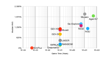
Figure 2: SOTA algorithms of Atari 57 games on mean and median HNS (%) and game time (year).

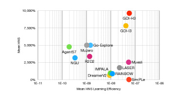
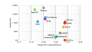
Figure 3: SOTA algorithms of Atari 57 games on mean and median HNS (%) and corresponding learning efficiency calculated by $\frac{\text{MEAN HNS/MEDIAN HNS}}{\text{TRAINING FRAMES}}$.

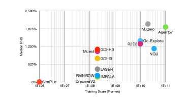
Figure 4: SOTA algorithms of Atari 57 games on mean and median HNS (%) and corresponding training scale.

D.2 RL Benchmarks on HWRNS

We report several milestones of Atari benchmarks on Human World Records Normalized Score (HWRNS), including DQN (Mnih et al., 2015), RAINBOW (Hessel et al., 2017), IMPALA (Espeholt et al., 2018), LASER (Schmitt et al., 2020), R2D2 (Kapturowski et al., 2018), NGU (Badia et al., 2020b), Agent57 (Badia et al., 2020a), Go-Explore (Ecoffet et al., 2019), MuZero (Schrittwieser et al., 2020), DreamerV2 (Hafner et al., 2020), SimPLe (Kaiser et al., 2019) and Musile (Hessel et al., 2021). We summary mean HWRNS and median HWRNS of these algorithms marked with their game time (year), learning efficiency and training scale in Fig 5, 6 and 7.

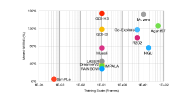
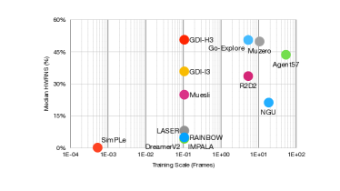
Figure 5: SOTA algorithms of Atari 57 games on mean and median HWRNS (%) and corresponding game time (year).

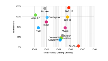
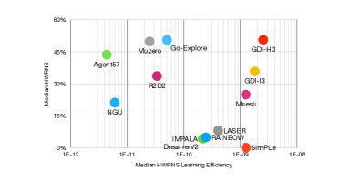
Figure 6: SOTA algorithms of Atari 57 games on mean and median HWRNS (%) and corresponding learning efficiency calculated by $\frac{\text{MEAN HWRNS/MEDIAN HWRNS}}{\text{TRAINING FRAMES}}$.

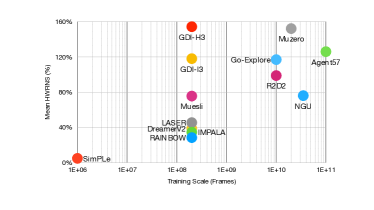
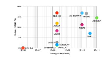
Figure 7: SOTA algorithms of Atari 57 games on mean and median HWRNS (%) and corresponding training scale.

D.3 RL Benchmarks on SABER

We report several milestones of Atari benchmarks on Standardized Atari BEnchmark for RL (SABER), including DQN (Mnih et al., 2015), RAINBOW (Hessel et al., 2017), IMPALA (Espeholt et al., 2018), LASER (Schmitt et al., 2020), R2D2 (Kapturowski et al., 2018), NGU (Badia et al., 2020b), Agent57 (Badia et al., 2020a), Go-Explore (Ecoffet et al., 2019), MuZero (Schrittwieser et al., 2020), DreamerV2 (Hafner et al., 2020), SimPLe (Kaiser et al., 2019) and Musile (Hessel et al., 2021). We summary mean SABER and median SABER of these algorithms marked with their game time (year), learning efficiency and training scale in Fig 8, 9 and 10.

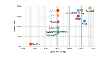
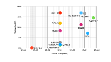
Figure 8: SOTA algorithms of Atari 57 games on mean and median SABER (%) and corresponding game time (year).

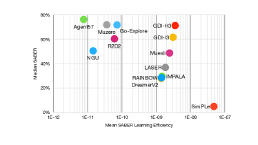
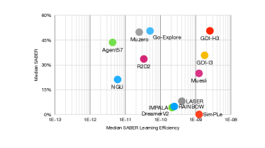
Figure 9: SOTA algorithms of Atari 57 games on mean and median SABER (%) and corresponding learning efficiency calculated by $\frac{\text{MEAN SABER/MEDIAN SABER}}{\text{TRAINING FRAMES}}$.

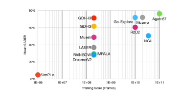
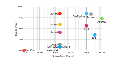
Figure 10: SOTA algorithms of Atari 57 games on mean and median SABER (%) and corresponding training scale.

D.4 RL Benchmarks on HWRB

We report several milestones of Atari benchmarks on HWRB, including DQN (Mnih et al., 2015), RAINBOW (Hessel et al., 2017), IMPALA (Espeholt et al., 2018), LASER (Schmitt et al., 2020), R2D2 (Kapturowski et al., 2018), NGU (Badia et al., 2020b), Agent57 (Badia et al., 2020a), Go-Explore (Ecoffet et al., 2019), MuZero (Schrittwieser et al., 2020), DreamerV2 (Hafner et al., 2020), SimPLe (Kaiser et al., 2019) and Musile (Hessel et al., 2021). We summary HWRB of these algorithms marked with their game time (year), learning efficiency and training scale in Fig 11.

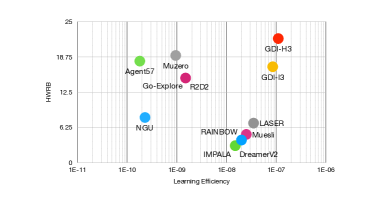
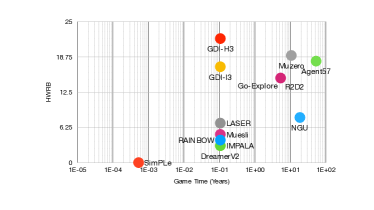
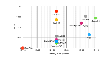
Figure 11: SOTA algorithms of Atari 57 games on HWRB. HWRB of SimPLe is 0, so it’s not shown in the up-right figure.

Appendix E Theoretical Proof

For a monotonic sequence of numbers which satisfies $a=x_{0}<x_{1}<\dots<x_{n}<b$, we call it a split of interval $[a,b]$.

Lemma 1 (Discretized Upper Triangular Transport Inequality for Increasing Functions in $\mathbf{R}^{1}$).

Assume $\mu$ is a continuous probability measure supported on $[0,1]$. Let $0=x_{0}<x_{1}<\dots<x_{n}<1$ to be any split of $[0,1]$. Define $\tilde{\mu}(x_{i})=\mu([x_{i},x_{i+1}))$. Define

$$\tilde{\beta}(x_{i})=\tilde{\mu}(x_{i})\exp(x_{i})/Z,\ Z=\sum_{i}\tilde{\mu}(x_{i})\exp(x_{i}).$$

Then there exists a probability measure $\gamma:\{x_{i}\}_{i=0,\dots,n}\times\{x_{i}\}_{i=0,\dots,n}\rightarrow[0,1]$, s.t.

$$\left\{\begin{aligned} &\sum_{j}\gamma(x_{i},y_{j})=\tilde{\mu}(x_{i}),&&\ i=0,\dots,n;\\ &\sum_{i}\gamma(x_{i},y_{j})=\tilde{\beta}(y_{j}),&&\ j=0,\dots,n;\\ &\gamma(x_{i},y_{j})=0,&&\ i>j.\\ \end{aligned}\right.$$ (5)

Then for any monotonic increasing function $f:\{x_{i}\}_{i=0,\dots,n}\rightarrow$ R, we have

$$\textbf{E}_{\tilde{\mu}}[f]\leq\textbf{E}_{\tilde{\beta}}[f].$$

Proof of Lemma 1.

For any couple of measures $(\mu,\beta)$, we say the couple satisfies Upper Triangular Transport Condition (UTTC), if there exists $\gamma$ s.t. (5) holds.

Given $0=x_{0}<x_{1}<\dots<x_{n}<1$, we prove the existence of $\gamma$ by induction.

Define

$$\tilde{\mu}_{m}(x_{i})=\left\{\begin{aligned} &\mu([x_{i},x_{i+1})),&&i<m,\\ &\mu([x_{i},1)),&&i=m,\\ &0,&&i>m.\end{aligned}\right.$$

Define

$$\tilde{\beta}_{m}(x_{i})=\tilde{\mu}_{m}(x_{i})\exp(x_{i})/Z_{m},\ Z_{m}=\sum_{i}\tilde{\mu}_{m}(x_{i})\exp(x_{i}).$$

Noting if we prove that $(\tilde{\mu}_{m},\tilde{\beta}_{m})$ satisfies UTTC for $m=n$, it’s equivalent to prove the existence of $\gamma$ in (5).

To clarify the proof, we use $x_{i}$ to represent the point for $\tilde{\mu}$-axis in coupling and $y_{j}$ to represent the point for $\tilde{\beta}$-axis, but they are actually identical, i.e. $x_{i}=y_{j}$ when $i=j$.

When $m=0$, it’s obvious that $(\tilde{\mu}_{0},\tilde{\beta}_{0})$ satisfies UTTC, as

$$\gamma_{0}(x_{i},y_{j})=\left\{\begin{aligned} &1,\ i=0,j=0,\\ &0,\ else.\end{aligned}\right.$$

Assume UTTC holds for $m$, i.e. there exists $\gamma_{m}$ s.t. $(\tilde{\mu}_{m},\tilde{\beta}_{m})$ satisfies UTTC, we want to prove it also holds for $m+1$.

By definition of $\tilde{\mu}_{m}$, we have

$$\left\{\begin{aligned} &\tilde{\mu}_{m}(x_{i})=\tilde{\mu}_{m+1}(x_{i}),&&i<m,\\ &\tilde{\mu}_{m}(x_{i})=\tilde{\mu}_{m+1}(x_{i})+\tilde{\mu}_{m+1}(x_{i+1}),&&i=m,\\ &\tilde{\mu}_{m}(x_{m+1})=\tilde{\mu}_{m}(x_{i})=\tilde{\mu}_{m+1}(x_{i})=0,&&i>m+1.\\ \end{aligned}\right.$$

By definition of $\tilde{\beta}_{m}$, we have

$$\left\{\begin{aligned} &\tilde{\beta}_{m}(x_{i})=\tilde{\beta}_{m+1}(x_{i})\cdot\frac{Z_{m+1}}{Z_{m}},&&i<m,\\ &\tilde{\beta}_{m}(x_{i})=\left(\tilde{\beta}_{m+1}(x_{i})+\tilde{\beta}_{m+1}(x_{i+1})\exp(x_{i}-x_{i+1})\right)\cdot\frac{Z_{m+1}}{Z_{m}},&&i=m,\\ &\tilde{\beta}_{m}(x_{m+1})=\tilde{\beta}_{m}(x_{i})=\tilde{\beta}_{m+1}(x_{i})=0,&&i>m+1.\\ \end{aligned}\right.$$

Multiplying $\gamma_{m}$ by $\frac{Z_{m}}{Z_{m+1}}$, we get the following UTTC

$$\left\{\begin{aligned} &\sum_{j}\frac{Z_{m}}{Z_{m+1}}\gamma_{m}(x_{i},y_{j})=\frac{Z_{m}}{Z_{m+1}}\tilde{\mu}_{m+1}(x_{i}),&&\ i<m;\\ &\sum_{j}\frac{Z_{m}}{Z_{m+1}}\gamma_{m}(x_{i},y_{j})=\frac{Z_{m}}{Z_{m+1}}(\tilde{\mu}_{m+1}(x_{i})+\tilde{\mu}_{m+1}(x_{i+1})),&&\ i=m;\\ &\sum_{j}\frac{Z_{m}}{Z_{m+1}}\gamma_{m}(x_{i},y_{j})=0,&&\ i=m+1;\\ &\sum_{j}\frac{Z_{m}}{Z_{m+1}}\gamma_{m}(x_{i},y_{j})=\tilde{\mu}_{m+1}(x_{i})=0,&&\ i>m+1;\\ &\sum_{i}\frac{Z_{m}}{Z_{m+1}}\gamma_{m}(x_{i},y_{j})=\tilde{\beta}_{m+1}(y_{j}),&&\ j<m;\\ &\sum_{i}\frac{Z_{m}}{Z_{m+1}}\gamma_{m}(x_{i},y_{j})=\tilde{\beta}_{m+1}(y_{i})+\tilde{\beta}_{m+1}(y_{j+1})\exp(y_{j}-y_{j+1}),&&\ j=m;\\ &\sum_{i}\frac{Z_{m}}{Z_{m+1}}\gamma_{m}(x_{i},y_{j})=0,&&\ j=m+1;\\ &\sum_{i}\frac{Z_{m}}{Z_{m+1}}\gamma_{m}(x_{i},y_{j})=\tilde{\beta}_{m+1}(y_{j})=0,&&\ j>m+1;\\ &\frac{Z_{m}}{Z_{m+1}}\gamma_{m}(x_{i},y_{j})=0,&&\ i>j.\\ \end{aligned}\right.$$

By definition of $Z_{m}$,

$$Z_{m+1}-Z_{m}=\tilde{\mu}_{m+1}(x_{m+1})(\exp(x_{m+1})-\exp(x_{m}))>0,$$ (6)

so we have $\frac{Z_{m}}{Z_{m+1}}\tilde{\mu}_{m+1}(x_{i})<\tilde{\mu}_{m+1}(x_{i})$.

Noticing that $\tilde{\beta}_{m+1}(y_{i+1})\exp(y_{i}-y_{i+1})<\tilde{\beta}_{m+1}(y_{i+1})$ and $\frac{Z_{m}}{Z_{m+1}}\tilde{\mu}_{m+1}(x_{i})<\tilde{\mu}_{m+1}(x_{i})$, we decompose the measure of $\frac{Z_{m}}{Z_{m+1}}\gamma_{m}$ at $(x_{i},y_{m})$ to $(x_{i},y_{m}),(x_{i},y_{m+1})$ for $i=0,\dots,m-1$, and complement a positive measure at $(x_{i},y_{m+1})$ to make up the difference between $\frac{Z_{m}}{Z_{m+1}}\tilde{\mu}_{m+1}(x_{i})$ and $\tilde{\mu}_{m+1}(x_{i})$. For $i=m$, we decompose the measure at $(x_{m},y_{m})$ to $(x_{m},y_{m}),(x_{m},y_{m+1}),(x_{m+1},y_{m+1})$ and also complement a proper positive measure.

Now we define $\gamma_{m+1}$ by

$$\left\{\begin{aligned} &\gamma_{m+1}(x_{i},y_{j})=\frac{Z_{m}}{Z_{m+1}}\gamma_{m}(x_{i},y_{j}),\qquad\qquad\qquad\qquad\quad i<m\ and\ j<m,\\ &\gamma_{m+1}(x_{i},y_{j})=\left(\frac{Z_{m}}{Z_{m+1}}\gamma_{m}(x_{i},y_{j})+\frac{Z_{m+1}-Z_{m}}{Z_{m+1}}\tilde{\mu}_{m+1}(x_{i})\right)\\ &\ \quad\qquad\qquad\quad\cdot\frac{\tilde{\beta}_{m+1}(y_{j})}{\tilde{\beta}_{m+1}(y_{j})+\tilde{\beta}_{m+1}(y_{j+1})},\qquad\qquad\quad i<m\ and\ j=m,\\ &\gamma_{m+1}(x_{i},y_{j})=\left(\frac{Z_{m}}{Z_{m+1}}\gamma_{m}(x_{i},y_{j})+\frac{Z_{m+1}-Z_{m}}{Z_{m+1}}\tilde{\mu}_{m+1}(x_{i})\right)\\ &\ \quad\qquad\qquad\quad\cdot\frac{\tilde{\beta}_{m+1}(y_{j+1})}{\tilde{\beta}_{m+1}(y_{j})+\tilde{\beta}_{m+1}(y_{j+1})},\quad\qquad\ i<m\ and\ j=m+1,\\ &\gamma_{m+1}(x_{i},y_{j})=0,\quad\qquad\qquad\qquad\qquad i>j\ or\ i>m+1\ or\ j>m+1,\\ &\gamma_{m+1}(x_{m},y_{m})=u,\\ &\gamma_{m+1}(x_{m},y_{m+1})=v,\\ &\gamma_{m+1}(x_{m+1},y_{m+1})=w,\\ \end{aligned}\right.$$

where we assume $u,v,w$ to be the solution of the following equations

$$\left\{\begin{aligned} &u+v+w=\tilde{\mu}_{m+1}(x_{m})+\tilde{\mu}_{m+1}(x_{m+1}),\\ &\frac{w}{u+v}=\frac{\tilde{\mu}_{m+1}(x_{m+1})}{\tilde{\mu}_{m+1}(x_{m})},\\ &\frac{v+w}{u}=\frac{\tilde{\beta}_{m+1}(x_{m+1})}{\tilde{\beta}_{m+1}(x_{m})},\\ &u,v,w\geq 0.\\ \end{aligned}\right.$$ (7)

It’s obvious that

$$\left\{\begin{aligned} &\sum_{j}\gamma_{m+1}(x_{i},y_{j})=\tilde{\mu}_{m+1}(x_{i})=0,&&\ i>m+1,\\ &\sum_{i}\gamma_{m+1}(x_{i},y_{j})=\tilde{\beta}_{m+1}(y_{j})=0,&&\ j>m+1,\\ &\gamma(x_{i},y_{j})=0,&&\ i>j.\\ \end{aligned}\right.$$

For $j<m$, since $\sum_{i}\frac{Z_{m}}{Z_{m+1}}\gamma_{m}(x_{i},y_{j})=\tilde{\beta}_{m+1}(y_{j})$, we have

$$\sum_{i}\gamma_{m+1}(x_{i},y_{j})=\tilde{\beta}_{m+1}(y_{j}),\ j<m.$$

For $i<m$, since $\sum_{j}\frac{Z_{m}}{Z_{m+1}}\gamma_{m}(x_{i},y_{j})=\frac{Z_{m}}{Z_{m+1}}\tilde{\mu}_{m+1}(x_{i})<\tilde{\mu}_{m+1}(x_{i})$, we add $\frac{Z_{m+1}-Z_{m}}{Z_{m+1}}\tilde{\mu}_{m+1}(x_{i})\frac{\tilde{\beta}_{m+1}(y_{m})}{\tilde{\beta}_{m+1}(y_{m})+\tilde{\beta}_{m+1}(y_{m+1})}$, $\frac{Z_{m+1}-Z_{m}}{Z_{m+1}}\tilde{\mu}_{m+1}(x_{i})\frac{\tilde{\beta}_{m+1}(y_{m+1})}{\tilde{\beta}_{m+1}(y_{m})+\tilde{\beta}_{m+1}(y_{m+1})}$ to $\gamma_{m+1}(x_{i},y_{m})$, $\gamma_{m+1}(x_{i},y_{m+1})$, respectively. So we have

$$\sum_{j}\gamma_{m+1}(x_{i},y_{j})=\tilde{\mu}_{m+1}(x_{i}),\ i<m.$$

For $i=m,m+1$, since assumption (7) holds, we have $u+v+w=\tilde{\mu}_{m+1}(x_{m})+\tilde{\mu}_{m+1}(x_{m+1}),\frac{w}{u+v}=\frac{\tilde{\mu}_{m+1}(x_{m+1})}{\tilde{\mu}_{m+1}(x_{m})}$, it’s obvious that $u+v=\tilde{\mu}_{m+1}(x_{m}),w=\tilde{\mu}_{m+1}(x_{m+1})$, which is

$$\sum_{j}\gamma_{m+1}(x_{i},y_{j})=\tilde{\mu}_{m+1}(x_{i}),\ i=m,m+1.$$

For $j=m,m+1$, we firstly have

$$\sum_{j=m,m+1}\sum_{i}\gamma_{m+1}(x_{i},y_{j}) =\sum_{j}\sum_{i}\gamma_{m+1}(x_{i},y_{j})-\sum_{j\neq m,m+1}\sum_{i}\gamma_{m+1}(x_{i},y_{j})$$

$$=\sum_{i}\sum_{j}\gamma_{m+1}(x_{i},y_{j})-\sum_{j\neq m,m+1}\tilde{\beta}_{m+1}(y_{j})$$

$$=\sum_{i}\tilde{\mu}_{m+1}(x_{i})-\sum_{j\neq m,m+1}\tilde{\beta}_{m+1}(y_{j})$$

$$=1-(1-\tilde{\beta}_{m+1}(y_{m})-\tilde{\beta}_{m+1}(y_{m+1}))$$

$$=\tilde{\beta}_{m+1}(y_{m})+\tilde{\beta}_{m+1}(y_{m+1}).$$

By definition of $\gamma_{m+1}$, we know $\frac{\gamma_{m+1}(x_{i},y_{m})}{\gamma_{m}(x_{i},y_{m})}=\frac{\tilde{\beta}_{m+1}(x_{m+1})}{\tilde{\beta}_{m+1}(x_{m})}$ for $i<m$. By assumption (7), we know $\frac{v+w}{u}=\frac{\tilde{\beta}_{m+1}(x_{m+1})}{\tilde{\beta}_{m+1}(x_{m})}$. Combining three equations above together, we have

$$\sum_{i}\gamma_{m+1}(x_{i},y_{j})=\tilde{\beta}_{m+1}(y_{j}),\ j=m,m+1.$$

Now we only need to prove assumption (7) holds. With linear algebra, we solve (7) and have

$$\left\{\begin{aligned} &u=w\frac{1+\frac{\tilde{\mu}_{m+1}(x_{m+1})}{\tilde{\mu}_{m+1}(x_{m})}}{\frac{\tilde{\mu}_{m+1}(x_{m+1})}{\tilde{\mu}_{m+1}(x_{m})}\left(1+\frac{\tilde{\beta}_{m+1}(x_{m+1})}{\tilde{\beta}_{m+1}(x_{m})}\right)},\\ &v=w\frac{\frac{\tilde{\beta}_{m+1}(x_{m+1})}{\tilde{\beta}_{m+1}(x_{m})}-\frac{\tilde{\mu}_{m+1}(x_{m+1})}{\tilde{\mu}_{m+1}(x_{m})}}{\frac{\tilde{\mu}_{m+1}(x_{m+1})}{\tilde{\mu}_{m+1}(x_{m})}\left(1+\frac{\tilde{\beta}_{m+1}(x_{m+1})}{\tilde{\beta}_{m+1}(x_{m})}\right)},\\ &w=\frac{\left(\tilde{\mu}_{m+1}(x_{m})+\tilde{\mu}_{m+1}(x_{m+1})\right)\frac{\tilde{\mu}_{m+1}(x_{m+1})}{\tilde{\mu}_{m+1}(x_{m})}\left(1+\frac{\tilde{\beta}_{m+1}(x_{m+1})}{\tilde{\beta}_{m+1}(x_{m})}\right)}{\left(1+\frac{\tilde{\mu}_{m+1}(x_{m+1})}{\tilde{\mu}_{m+1}(x_{m})}\right)\left(1+\frac{\tilde{\beta}_{m+1}(x_{m+1})}{\tilde{\beta}_{m+1}(x_{m})}\right)}.\\ \end{aligned}\right.$$

It’s obvious that $u,w\geq 0$. $v\geq 0$ also holds, because

$$\frac{\tilde{\beta}_{m+1}(x_{m+1})}{\tilde{\beta}_{m+1}(x_{m})}-\frac{\tilde{\mu}_{m+1}(x_{m+1})}{\tilde{\mu}_{m+1}(x_{m})} =\frac{\tilde{\mu}_{m+1}(x_{m+1})\exp(x_{m+1})}{\tilde{\mu}_{m+1}(x_{m})\exp(x_{m})}-\frac{\tilde{\mu}_{m+1}(x_{m+1})}{\tilde{\mu}_{m+1}(x_{m})}$$ (8)

$$=\frac{\tilde{\mu}_{m+1}(x_{m+1})}{\tilde{\mu}_{m+1}(x_{m})}\left(\exp(x_{m+1}-x_{m})-1\right)\geq 0.$$

So we can find a proper solution of assumption (7).

So $\gamma_{m+1}$ defined above satisfies UTTC for $(\tilde{\mu}_{m+1},\tilde{\beta}_{m+1})$.

By induction, for any $0=x_{0}<x_{1}<\dots<x_{n}<1$, there exists $\gamma$ s.t. UTTC (5) holds for $(\tilde{\mu},\tilde{\beta})$.

Then for any monotonic increasing function, since $\gamma(x_{i},y_{j})=0$ when $i>j$, we know $\gamma(x_{i},y_{j})f(x_{i})\leq\gamma(x_{i},y_{j})f(y_{j})$. Hence we have

$$\textbf{E}_{\tilde{\mu}}[f] =\sum_{i}\tilde{\mu}(x_{i})f(x_{i})=\sum_{i}\sum_{j}\gamma(x_{i},y_{j})f(x_{i})$$

$$\leq\sum_{i}\sum_{j}\gamma(x_{i},y_{j})f(y_{j})$$

$$=\sum_{j}\sum_{i}\gamma(x_{i},y_{j})f(y_{j})$$

$$=\sum_{j}\tilde{\beta}(y_{j})f(y_{j})=\textbf{E}_{\tilde{\beta}}[f].$$

∎

Lemma 2 (Discretized Upper Triangular Transport Inequality for Co-Monotonic Functions in $\mathbf{R}^{1}$).

Assume $\mu$ is a continuous probability measure supported on $[0,1]$. Let $0=x_{0}<x_{1}<\dots<x_{n}<1$ to be any split of $[0,1]$. Let $f,g:\{x_{i}\}_{i=0,\dots,n}\rightarrow$ R to be two co-monotonic functions that satisfy

$$(f(x_{i})-f(x_{j}))\cdot(g(x_{i})-g(x_{j}))\geq 0,\ \forall\ i,j.$$

Define $\tilde{\mu}(x_{i})=\mu([x_{i},x_{i+1}))$. Define

$$\tilde{\beta}(x_{i})=\tilde{\mu}(x_{i})\exp(g(x_{i}))/Z,\ Z=\sum_{i}\tilde{\mu}(x_{i})\exp(g(x_{i})).$$

Then we have

$$\textbf{E}_{\tilde{\mu}}[f]\leq\textbf{E}_{\tilde{\beta}}[f].$$

Proof of Lemma 2.

If the Upper Triangular Transport Condition (UTTC) holds for $(\tilde{\mu},\tilde{\beta})$, i.e. there exists a probability measure $\gamma:\{x_{i}\}_{i=0,\dots,n}\times\{x_{i}\}_{i=0,\dots,n}\rightarrow[0,1]$, s.t.

$$\left\{\begin{aligned} &\sum_{j}\gamma(x_{i},y_{j})=\tilde{\mu}(x_{i}),&&\ i=0,\dots,n;\\ &\sum_{i}\gamma(x_{i},y_{j})=\tilde{\beta}(y_{j}),&&\ j=0,\dots,n;\\ &\gamma(x_{i},y_{j})=0,&&\ g(x_{i})>g(y_{j}),\\ \end{aligned}\right.$$

then we finish the proof by

$$\textbf{E}_{\tilde{\mu}}[f] =\sum_{i}\tilde{\mu}(x_{i})f(x_{i})=\sum_{i}\sum_{j}\gamma(x_{i},y_{j})f(x_{i})$$

$$\leq\sum_{i}\sum_{j}\gamma(x_{i},y_{j})f(y_{j})$$

$$=\sum_{j}\sum_{i}\gamma(x_{i},y_{j})f(y_{j})$$

$$=\sum_{j}\tilde{\beta}(y_{j})f(y_{j})=\textbf{E}_{\tilde{\beta}}[f],$$

where $\gamma(x_{i},y_{j})f(x_{i})\leq\gamma(x_{i},y_{j})f(y_{j})$ is because of $\gamma(x_{i},y_{j})=0,\ g(x_{i})>g(y_{j})$ and $(f(x_{i})-f(x_{j}))\cdot(g(x_{i})-g(x_{j}))\geq 0$.

Now we only need to prove UTTC holds for $(\tilde{\mu},\tilde{\beta})$.

Given $0=x_{0}<x_{1}<\dots<x_{n}<1$, we prove the existence of $\gamma$ by induction. With $g$ to be the transition function in the definition of $\tilde{\beta}$, we mimic the proof of Lemma 1 and sort $(x_{0},\dots,x_{n})$ in the increasing order of $g$, which is

$$g(x_{k_{0}})\leq g(x_{k_{1}})\leq\dots\leq g(x_{k_{n}}).$$

Define

$$\tilde{\mu}_{m}(x_{k_{i}})=\left\{\begin{aligned} &\mu([x_{k_{i}},\min\{1,x_{k_{l}}|\ x_{k_{l}}>x_{k_{i}},l\leq m\})),&&i\leq m,\ x_{k_{i}}\neq\min\{x_{k_{l}}|\ l\leq m\},\\ &\mu([0,\min\{1,x_{k_{l}}|\ x_{k_{l}}>x_{k_{i}},l\leq m\})),&&i\leq m,\ x_{k_{i}}=\min\{x_{k_{l}}|\ l\leq m\},\\ &0,&&i>m.\end{aligned}\right.$$

Define

$$\tilde{\beta}_{m}(x_{k_{i}})=\tilde{\mu}_{m}(x_{k_{i}})\exp(g(x_{k_{i}}))/Z_{m},\ Z_{m}=\sum_{i}\tilde{\mu}_{m}(x_{k_{i}})\exp(g(x_{k_{i}})).$$

To clarify the proof, we use $x_{k_{i}}$ to represent the point for $\tilde{\mu}$-axis in coupling and $y_{k_{j}}$ to represent the point for $\tilde{\beta}$-axis, but they are actually identical, i.e. $x_{k_{i}}=y_{k_{j}}$ when $i=j$.

When $m=0$, it’s obvious that $(\tilde{\mu}_{0},\tilde{\beta}_{0})$ satisfies UTTC, as

$$\gamma_{0}(x_{k_{i}},y_{k_{j}})=\left\{\begin{aligned} &1,&&\ i=0,j=0,\\ &0,&&\ else.\\ \end{aligned}\right.$$

Assume UTTC holds for $m$, i.e. there exists $\gamma_{m}$ s.t. $(\tilde{\mu}_{m},\tilde{\beta}_{m})$ satisfies UTTC, we want to prove it also holds for $m+1$.

When $x_{k_{m+1}}>\min\{x_{k_{l}}|\ l\leq m\}$, let $x_{k^{*}}=\max\{x_{k_{l}}|\ x_{k_{l}}<x_{k_{m+1}},l\leq m\}$ to be the closest left neighbor of $x_{k_{m+1}}$ in $\{x_{k_{l}}|\ l\leq m\}$. Then we have $\tilde{\mu}_{m}(x_{k^{*}})=\tilde{\mu}_{m+1}(x_{k^{*}})+\tilde{\mu}_{m+1}(x_{k^{m+1}})$.

When $x_{k_{m+1}}<\min\{x_{k_{l}}|\ l\leq m\}$, let $x_{k^{*}}=\min\{x_{k_{l}}|\ l\leq m\}$ to be the leftmost point in $\{x_{k_{l}}|\ l\leq m\}$. Then we have $\tilde{\mu}_{m}(x_{k^{*}})=\tilde{\mu}_{m+1}(x_{k^{*}})+\tilde{\mu}_{m+1}(x_{k^{m+1}})$.

In either case, we always have $\tilde{\mu}_{m}(x_{k^{*}})=\tilde{\mu}_{m+1}(x_{k^{*}})+\tilde{\mu}_{m+1}(x_{k_{m+1}})$. By definition of $\tilde{\mu}_{m}$ and $\tilde{\beta}_{m}$, we have

$$\left\{\begin{aligned} &\tilde{\mu}_{m}(x_{k_{i}})=\tilde{\mu}_{m+1}(x_{k_{i}}),&&i\leq m,\ k_{i}\neq k^{*},\\ &\tilde{\mu}_{m}(x_{k_{i}})=\tilde{\mu}_{m+1}(x_{k_{i}})+\tilde{\mu}_{m+1}(x_{k_{m+1}}),&&i\leq m,\ k_{i}=k^{*},\\ &\tilde{\mu}_{m}(x_{k_{m+1}})=\tilde{\mu}_{m}(x_{k_{i}})=\tilde{\mu}_{m+1}(x_{k_{i}})=0,&&i>m+1,\\ \end{aligned}\right.$$

$$\left\{\begin{aligned} &\tilde{\beta}_{m}(x_{k_{i}})=\tilde{\beta}_{m+1}(x_{k_{i}})\cdot\frac{Z_{m+1}}{Z_{m}},&&i\leq m,\ k_{i}\neq k^{*},\\ &\tilde{\beta}_{m}(x_{k_{i}})=\left(\tilde{\beta}_{m+1}(x_{k_{i}})+\tilde{\beta}_{m+1}(x_{k_{m+1}})\exp\left(g(x_{k_{i}})-g(x_{k_{m+1}})\right)\right)\cdot\frac{Z_{m+1}}{Z_{m}},&&i\leq m,\ k_{i}=k^{*},\\ &\tilde{\beta}_{m}(x_{m+1})=\tilde{\beta}_{m}(x_{i})=\tilde{\beta}_{m+1}(x_{i})=0,&&i>m+1.\\ \end{aligned}\right.$$

If $g(x_{k^{*}})=g(x_{k_{m+1}})$, it’s easy to check that $\frac{\tilde{\mu}_{m+1}(x_{k_{m+1}})}{\tilde{\mu}_{m+1}(x_{k^{*}})}=\frac{\tilde{\beta}_{m+1}(x_{k_{m+1}})}{\tilde{\beta}_{m+1}(x_{k^{*}})}$, we can simply define the following $\gamma_{m+1}$ which achieves UTTC for $(\tilde{\mu}_{m+1},\tilde{\beta}_{m+1})$:

$$\left\{\begin{aligned} &\gamma_{m+1}(x_{k^{*}},y_{k_{j}})=\gamma_{m}(x_{k^{*}},y_{k_{j}})\frac{\tilde{\mu}_{m+1}(x_{k^{*}})}{\tilde{\mu}_{m+1}(x_{k^{*}})+\tilde{\mu}_{m+1}(x_{k_{m+1}})},&&\ j\leq m,\ k_{j}\neq k^{*},\\ &\gamma_{m+1}(x_{k_{m+1}},y_{k_{j}})=\gamma_{m}(x_{k_{m+1}},y_{k_{j}})\frac{\tilde{\mu}_{m+1}(x_{k_{m+1}})}{\tilde{\mu}_{m+1}(x_{k^{*}})+\tilde{\mu}_{m+1}(x_{k_{m+1}})},&&\ j\leq m,\ k_{j}\neq k^{*},\\ &\gamma_{m+1}(x_{k_{i}},y_{k^{*}})=\gamma_{m}(x_{k_{i}},y_{k^{*}})\frac{\tilde{\beta}_{m+1}(y_{k^{*}})}{\tilde{\beta}_{m+1}(y_{k^{*}})+\tilde{\beta}_{m+1}(y_{k_{m+1}})},&&\ i\leq m,\ k_{i}\neq k^{*},\\ &\gamma_{m+1}(x_{k_{i}},y_{k_{m+1}})=\gamma_{m}(x_{k_{i}},y_{k_{m+1}})\frac{\tilde{\beta}_{m+1}(y_{k_{m+1}})}{\tilde{\beta}_{m+1}(y_{k^{*}})+\tilde{\mu}_{m+1}(x_{k_{m+1}})},&&\ i\leq m,\ k_{i}\neq k^{*},\\ &\gamma_{m+1}(x_{k^{*}},y_{k^{*}})=\gamma_{m}(x_{k^{*}},y_{k^{*}})\frac{\tilde{\mu}_{m+1}(x_{k^{*}})}{\tilde{\mu}_{m+1}(x_{k^{*}})+\tilde{\mu}_{m+1}(x_{k_{m+1}})},&&\\ &\gamma_{m+1}(x_{k_{m+1}},y_{k_{m+1}})=\gamma_{m}(x_{k_{m+1}},y_{k_{m+1}})\frac{\tilde{\mu}_{m+1}(x_{k_{m+1}})}{\tilde{\mu}_{m+1}(x_{k^{*}})+\tilde{\mu}_{m+1}(x_{k_{m+1}})},\\ &\gamma_{m+1}(x_{k_{i}},y_{k_{j}})=0,&&\ others.\end{aligned}\right.$$

If $g(x_{k^{*}})<g(x_{k_{m+1}})$, recalling the proof of Lemma 1, it’s crucial to prove inequalities (6) and (8). Inequality (6) guarantees that $\frac{Z_{m}}{Z_{m+1}}<1$, so we can shrinkage $\gamma_{m}$ entrywise by $\frac{Z_{m}}{Z_{m+1}}$ and add some proper measure at proper points. Inequality (8) guarantees that $(x_{m},y_{m})$ can be decomposed to $(x_{m},y_{m})$, $(x_{m},y_{m+1})$, $(x_{m+1},y_{m+1})$. Following the idea, we check that

$$Z_{m+1}-Z_{m}=\tilde{\mu}_{m+1}(x_{k_{m+1}})\left(\exp(g(x_{k_{m+1}})-g(x_{k^{*}}))\right)>0,$$

$$\frac{\tilde{\beta}_{m+1}(x_{k_{m+1}})}{\tilde{\beta}_{m+1}(x_{k^{*}})}-\frac{\tilde{\mu}_{m+1}(x_{k_{m+1}})}{\tilde{\mu}_{m+1}(x_{k^{*}})} =\frac{\tilde{\mu}_{m+1}(x_{k_{m+1}})\exp(g(x_{k_{m+1}}))}{\tilde{\mu}_{m+1}(x_{k^{*}})\exp(g(x_{k^{*}}))}-\frac{\tilde{\mu}_{m+1}(x_{k_{m+1}})}{\tilde{\mu}_{m+1}(x_{k^{*}})}$$

$$=\frac{\tilde{\mu}_{m+1}(x_{k_{m+1}})}{\tilde{\mu}_{m+1}(x_{k^{*}})}\left(\exp(g(x_{k_{m+1}})-g(x_{k^{*}}))-1\right)>0.$$

Replacing $x_{m},x_{m+1}$ in the proof of Lemma 1 by $x_{k^{*}},x_{k_{m+1}}$, we can construct $\gamma_{m+1}$ all the same way as in the proof of Lemma 1.

By induction, we prove UTTC for $(\tilde{\mu},\tilde{\beta})$. The proof is done. ∎

Theorem 3 (Upper Triangular Transport Inequality for Co-Monotonic Functions in $\mathbf{R}^{1}$).

Assume $\mu$ is a continuous probability measure supported on $[0,1]$. Let $f,g:[0,1]\rightarrow$ R to be two co-monotonic functions that satisfy

$$(f(x)-f(y))\cdot(g(x)-g(y))\geq 0,\ \forall\ x,y\in[0,1].$$

$f$ is continuous. Define

$$\beta(x)=\mu(x)\exp(g(x))/Z,\ Z=\int_{[0,1]}\mu(x)\exp(g(x)).$$

Then we have

$$\textbf{E}_{\mu}[f]\leq\textbf{E}_{\beta}[f].$$

Proof of Theorem 3.

For $\forall\epsilon>0$, since $f$ is continuous, $f$ is uniformly continuous, so there exists $\delta>0$ s.t. $|f(x)-f(y)|<\epsilon,\forall x,y\in[0,1]$. We can split $[0,1]$ by $0<x_{0}<x_{1}<\dots<x_{n}<1$ s.t. $x_{i+1}-x_{i}<\delta$. Define $\tilde{\mu}$ and $\tilde{\beta}$ as in Lemma 2. Since $x_{i+1}-x_{i}<\delta$, by uniform continuity and the definition of the expectation, we have

$$|\textbf{E}_{\mu}[f]-\textbf{E}_{\tilde{\mu}}[f]|<\epsilon,\ |\textbf{E}_{\beta}[f]-\textbf{E}_{\tilde{\beta}}[f]|<\epsilon,$$

By Lemma 2, we have

$$\textbf{E}_{\tilde{\mu}}[f]\leq\textbf{E}_{\tilde{\beta}}[f].$$

So we have

$$\textbf{E}_{\mu}[f]<\textbf{E}_{\tilde{\mu}}[f]+\epsilon\leq\textbf{E}_{\tilde{\beta}}[f]+\epsilon<\textbf{E}_{\beta}[f]+2\epsilon.$$

Since $\epsilon$ is arbitrary, we prove $\textbf{E}_{\mu}[f]\leq\textbf{E}_{\beta}[f].$

∎

Lemma 3 (Discretized Upper Triangular Transport Inequality for Co-Monotonic Functions in $\mathbf{R}^{p}$).

Assume $\mu$ is a continuous probability measure supported on $[0,1]^{p}$. Let $0=x_{0}^{d}<x_{1}^{d}<\dots<x_{n}^{d}<1$ to be any split of $[0,1]$, $d=1,\dots,p$. Denote $\textbf{x}_{\textbf{i}}\overset{def}{=}(x_{i_{1}}^{1},\dots,x_{i_{p}}^{p})$. Define $\tilde{\mu}(\textbf{x}_{\textbf{i}})=\mu(\prod_{d=1,\dots,p}[x_{i_{d}}^{d},x_{i_{d}+1}^{d}))$. Let $f,g:\{\textbf{x}_{\textbf{i}}\}_{\textbf{i}\in\{0,\dots,n\}^{p}}\rightarrow$ R to be two co-monotonic functions that satisfy

$$(f(\textbf{x}_{\textbf{i}})-f(\textbf{x}_{\textbf{j}}))\cdot(g(\textbf{x}_{\textbf{i}})-g(\textbf{x}_{\textbf{j}}))\geq 0,\ \forall\ \textbf{i},\textbf{j}.$$

Define

$$\tilde{\beta}(\textbf{x}_{\textbf{i}})=\tilde{\mu}(\textbf{x}_{\textbf{i}})\exp(g(\textbf{x}_{\textbf{i}}))/Z,\ Z=\sum_{\textbf{i}}\tilde{\mu}(\textbf{x}_{\textbf{i}})\exp(g(\textbf{x}_{\textbf{i}})).$$

Then there exists a probability measure $\gamma:\{\textbf{x}_{\textbf{i}}\}_{\textbf{i}\in\{0,\dots,n\}^{p}}\times\{\textbf{x}_{\textbf{j}}\}_{\textbf{j}\in\{0,\dots,n\}^{p}}\rightarrow[0,1]$, s.t.

$$\sum_{\textbf{j}}\gamma(\textbf{x}_{\textbf{i}},\textbf{y}_{\textbf{j}}) =\tilde{\mu}(\textbf{x}_{\textbf{i}}),\ \forall\ \textbf{i};$$

$$\sum_{\textbf{i}}\gamma(\textbf{x}_{\textbf{i}},\textbf{y}_{\textbf{j}}) =\tilde{\beta}(\textbf{y}_{\textbf{j}}),\ \forall\ \textbf{j};$$

$$\gamma(\textbf{x}_{\textbf{i}},\textbf{y}_{\textbf{j}}) =0,\ g(\textbf{x}_{\textbf{i}})>g(\textbf{y}_{\textbf{j}}).$$

Then we have

$$\textbf{E}_{\tilde{\mu}}[f]\leq\textbf{E}_{\tilde{\beta}}[f].$$

Proof of Lemma 3.

The proof is almost identical to the proof of Lemma 2, except for the definition of $(\tilde{\mu}_{m},\tilde{\beta}_{m})$ in $\textbf{R}^{p}$.

Given $\{\textbf{x}_{\textbf{i}}\}_{\textbf{i}\in\{0,\dots,n\}^{p}}$, we sort $\textbf{x}_{\textbf{i}}$ in the increasing order of $g$, which is

$$g(\textbf{x}_{\textbf{k}_{0}})\leq g(\textbf{x}_{\textbf{k}_{1}})\leq\dots\leq g(\textbf{x}_{\textbf{k}_{(n+1)^{p}-1}}),$$

where $\{\textbf{k}_{i}\}_{i\in\{0,\dots,(n+1)^{p}-1\}}$ is a permutation of $\{\textbf{{i}}\}_{\textbf{i}\in\{0,\dots,n\}^{p}}$.

For $\textbf{i},\textbf{j}\in\{0,\dots,n\}^{p}$, we define the partial order $\textbf{i}<\textbf{j}$ on $\{0,\dots,n\}^{p}$, if

$$\exists 0\leq d_{0}\leq n,\ s.t.\ \textbf{i}_{d}\leq\textbf{j}_{d},\ \forall d<d_{0}\ and\ \textbf{i}_{d_{0}}<\textbf{j}_{d_{0}}.$$

It’s obvious that

$$\left\{\begin{aligned} &\forall\textbf{i}\in\{0,\dots,n\}^{p},\ \textbf{i}\nless\textbf{i},\\ &\forall\textbf{i},\textbf{j}\in\{0,\dots,n\}^{p},\ \textbf{i}<\textbf{j}\Rightarrow\textbf{j}\nless\textbf{i},\\ &\forall\textbf{i},\textbf{j},\textbf{k}\in\{0,\dots,n\}^{p},\ \textbf{i}<\textbf{j},\ \textbf{j}<\textbf{k}\Rightarrow\textbf{i}<\textbf{k}.\\ \end{aligned}\right.$$

We define $\textbf{i}=\textbf{j}$ if $\textbf{i}_{d}=\textbf{j}_{d},\,\forall\,0\leq d\leq n$. So we define the partial order relation, and we can further define the $\min$ function and the $\max$ function on $\{0,\dots,n\}^{p}$.

Now using this partial order relation, we define

$$\tilde{\mu}_{m}(\textbf{x}_{\textbf{k}_{i}})=\left\{\begin{aligned} &\sum_{\textbf{k}\geq\textbf{k}_{i},\textbf{k}<\min\{\textbf{k}_{l}|\textbf{k}_{l}>\textbf{k}_{i},l\leq m\}}\tilde{\mu}(\textbf{x}_{\textbf{k}}),&&\ i\leq m,\ \textbf{k}_{i}\neq\min\{\textbf{k}_{l}|\ l\leq m\},\\ &\sum_{\textbf{k}<\min\{\textbf{k}_{l}|\textbf{k}_{l}>\textbf{k}_{i},l\leq m\}}\tilde{\mu}(\textbf{x}_{\textbf{k}}),&&\ i\leq m,\ \textbf{k}_{i}=\min\{\textbf{k}_{l}|\ l\leq m\},\\ &0,&&\ i>m.\\ \end{aligned}\right.$$

With this definition of $\tilde{\mu}_{m}$, other parts are identical to the proof of Lemma 2. The proof is done.

∎

Theorem 4 (Upper Triangular Transport Inequality for Co-Monotonic Functions in $\mathbf{R}^{p}$).

Assume $\mu$ is a continuous probability measure supported on $[0,1]^{p}$. Denote $\textbf{x}\overset{def}{=}(x^{1},\dots,x^{p})$. Let $f,g:[0,1]^{p}\rightarrow$ R to be two co-monotonic functions that satisfy

$$(f(\textbf{x})-f(\textbf{y}))\cdot(g(\textbf{x})-g(\textbf{y}))\geq 0,\ \forall\ \textbf{x},\textbf{y}\in[0,1]^{p}.$$

$f$ is continuous. Define

$$\beta(\textbf{x})=\mu(\textbf{x})\exp(g(\textbf{x}))/Z,\ Z=\int_{[0,1]^{p}}\mu(\textbf{x})\exp(g(\textbf{x})).$$

Let $f,g:[0,1]^{p}\rightarrow$ R to be two co-monotonic functions that satisfy

$$(f(\textbf{x})-f(\textbf{y}))\cdot(g(\textbf{x})-g(\textbf{y}))\geq 0,\ \forall\ \textbf{x},\textbf{y}\in[0,1]^{p}.$$

Then we have

$$\textbf{E}_{\mu}[f]\leq\textbf{E}_{\beta}[f].$$

Proof of Theorem 4.

For $\forall\epsilon>0$, since $f$ is continuous, $f$ is uniformly continuous, so there exists $\delta>0$ s.t. $|f(\textbf{x})-f(\textbf{y})|<\epsilon,\forall\textbf{x},\textbf{y}\in[0,1]^{p}$. We can split $[0,1]$ by $0<x_{0}<x_{1}<\dots<x_{n}<1$ s.t. $x_{i+1}-x_{i}<\delta/\sqrt{p}$. Define $x_{i}^{d}=x_{i},\ \forall 0\leq d\leq p$. Define $\tilde{\mu}$ and $\tilde{\beta}$ as in Lemma 3. Since $x_{i+1}-x_{i}<\delta/\sqrt{p}$, $|(x_{i+1}^{0},\dots,x_{i+1}^{p})-(x_{i}^{0},\dots,x_{i}^{p})|<\delta$, by uniform continuity and the definition of the expectation, we have

$$|\textbf{E}_{\mu}[f]-\textbf{E}_{\tilde{\mu}}[f]|<\epsilon,\ |\textbf{E}_{\beta}[f]-\textbf{E}_{\tilde{\beta}}[f]|<\epsilon,$$

By Lemma 3, we have

$$\textbf{E}_{\tilde{\mu}}[f]\leq\textbf{E}_{\tilde{\beta}}[f].$$

So we have

$$\textbf{E}_{\mu}[f]<\textbf{E}_{\tilde{\mu}}[f]+\epsilon\leq\textbf{E}_{\tilde{\beta}}[f]+\epsilon<\textbf{E}_{\beta}[f]+2\epsilon.$$

Since $\epsilon$ is arbitrary, we prove $\textbf{E}_{\mu}[f]\leq\textbf{E}_{\beta}[f].$

∎

Lemma 4 (Performance Difference Lemma).

For any policies $\pi,\pi^{\prime}$ and any state $s_{0}$, we have

$$V^{\pi}(s_{0})-V^{\pi^{\prime}}(s_{0})=\frac{1}{1-\gamma}\textbf{E}_{s\sim d_{s_{0}}^{\pi}}\textbf{E}_{a\sim\pi(\cdot|s)}\left[A^{\pi^{\prime}}(s,a)\right].$$

Proof.

See (Kakade, Langford, 2002). ∎

Appendix F Algorithm Pseudocode

For completeness, we provide the implementation pseudocode of GDI-I³, which is shown in Algorithm 2.

$$\left\{\begin{aligned} &A=A_{\theta}\left(s_{t}\right),&&V=V_{\theta}\left(s_{t}\right),\\ &\bar{A}=A-E_{\pi}[A],&&Q=\bar{A}+V.\\ \end{aligned}\right.$$ (9)

$$\lambda=(\tau_{1},\tau_{2},\epsilon),\ \pi_{\theta_{\lambda}}=\varepsilon\cdot\underbrace{\operatorname{Softmax}\left(\frac{A}{\tau_{1}}\right)}_{Exploration}+(1-\varepsilon)\cdot\underbrace{\operatorname{Softmax}\left(\frac{A}{\tau_{2}}\right)}_{Exploitation}$$ (10)

Algorithm 2 GDI-I³ Algorithm.

  Initialize Parameter Server (PS) and Data Collector (DC).

  

  // LEARNER

  Initialize $d_{push}$.

  Initialize $\theta$ as Eq. (9) and (10).

  Initialize $count=0$.

  while $True$ do

     Load data from DC.

     Estimate $qs$ and $vs$ by proper off-policy algorithms.

         (For instance, ReTrace (B.1) for $qs$ and V-Trace (B.2) for $vs$.)

     Update $\theta$ via policy gradient and policy evaluation.

     if $count$ mod $d_{push}$ = 0 then

        Push $\theta$ to PS.

     end if

     $count\leftarrow count+1$.

  end while

  

  // ACTOR

  Initialize $d_{pull}$, $M$.

  Initialize $\theta$ as Eq. (9) and (10).

  Initialize $\{\mathcal{B}_{m}\}_{m=1,...,M}$ and sample $\lambda$ as in Algorithm 4.

  Initialize $count=0$, $G=0$.

  while $True$ do

     Calculate $\pi_{\theta_{\lambda}}(\cdot|s)$.

     Sample $a\sim\pi_{\theta_{\lambda}}(\cdot|s)$.

     $s,r,done\sim p(\cdot|s,a)$.

     $G\leftarrow G+r$.

     if $done$ then

        Update $\{\mathcal{B}_{m}\}_{m=1,...,M}$ with $(\lambda,G)$ as in Algorithm 4.

        Send data to DC and reset the environment.

        $G\leftarrow 0$.

        Sample $\lambda$ as in Algorithm 4

     end if

     if $count\mod d_{pull}$ = 0 then

        Pull $\theta$ from PS and update $\theta$.

     end if

     $count\leftarrow count+1$.

  end while

For completeness, we provide the implementation pseudocode of GDI-H³, which is shown in Algorithm 3.

$$\left\{\begin{aligned} &A_{1}=A_{\theta_{1}}\left(s_{t}\right),&&V_{1}=V_{\theta_{1}}\left(s_{t}\right),\\ &\bar{A}_{1}=A_{1}-E_{\pi}[A_{1}],&&Q_{1}=\bar{A}_{1}+V_{1}.\\ \end{aligned}\right.$$ (11)

$$\left\{\begin{aligned} &A_{2}=A_{\theta_{2}}\left(s_{t}\right),&&V_{2}=V_{\theta_{2}}\left(s_{t}\right),\\ &\bar{A}_{2}=A_{2}-E_{\pi}[A_{2}],&&Q_{2}=\bar{A}_{2}+V_{2}.\\ \end{aligned}\right.$$

$$\lambda=(\tau_{1},\tau_{2},\epsilon),\ \pi_{\theta_{\lambda}}=\varepsilon\cdot\operatorname{Softmax}\left(\frac{A_{1}}{\tau_{1}}\right)+(1-\varepsilon)\cdot\operatorname{Softmax}\left(\frac{A_{2}}{\tau_{2}}\right)$$ (12)

Algorithm 3 GDI-H³ Algorithm.

  Initialize Parameter Server (PS) and Data Collector (DC).

  

  // LEARNER

  Initialize $d_{push}$.

  Initialize $\theta$ as Eq. (11) and (12).

  Initialize $count=0$.

  while $True$ do

     Load data from DC.

     Estimate $qs_{1},qs_{2}$ and $vs_{1},vs_{2}$ by proper off-policy algorithms.

         (For instance, ReTrace (B.1) for $qs1,qs_{2}$ and V-Trace (B.2) for $vs_{1},vs_{2}$.)

     Update $\theta_{1},\theta_{2}$ via policy gradient and policy evaluation, respectively.

     if $count$ mod $d_{push}$ = 0 then

        Push $\theta_{1},\theta_{2}$ to PS.

     end if

     $count\leftarrow count+1$.

  end while

  

  // ACTOR

  Initialize $d_{pull}$, $M$.

  Initialize $\theta_{1},\theta_{2}$ as Eq. (11) and (12).

  Initialize $\{\mathcal{B}_{m}\}_{m=1,...,M}$ and sample $\lambda$ as in Algorithm 4.

  Initialize $count=0$, $G=0$.

  while $True$ do

     Calculate $\pi_{\theta_{\lambda}}(\cdot|s)$.

     Sample $a\sim\pi_{\theta_{\lambda}}(\cdot|s)$.

     $s,r,done\sim p(\cdot|s,a)$.

     $G\leftarrow G+r$.

     if $done$ then

        Update $\{\mathcal{B}_{m}\}_{m=1,...,M}$ with $(\lambda,G)$ as in Algorithm 4.

        Send data to DC and reset the environment.

        $G\leftarrow 0$.

        Sample $\lambda$ as in Algorithm 4

     end if

     if $count\mod d_{pull}$ = 0 then

        Pull $\theta$ from PS and update $\theta$.

     end if

     $count\leftarrow count+1$.

  end while

Appendix G Adaptive Controller Formalism

In practice, we use a Bandits Controller (BC) to adaptively control the behavior sampling distribution. More details on Bandits can be found in (Garivier, Moulines, 2008). The whole algorithm is shown in Algorithm 4. As the behavior policy can be parameterized and thus sampling behaviors from the policy space is equivalent to sampling parameters $x$ from parameter space.

Let’s firstly define a bandit as $B=Bandit(mode,l,r,lr,d,acc,ta,to,\textbf{w},\textbf{N})$.

• $mode$ is the mode of sampling, with two choices, $argmax$ and $random$, wherein $argmax$ greedily chooses the behaviors with top estimated value from the policy space, and $random$ samples behaviors according to a distribution calculated by $Softmax(V)$.

• $l$ is the left boundary of the parameter space, and each $x$ is clipped to $x=\max\{x,l\}$.

• $r$ is the right boundary of the parameter space, and each $x$ is clipped to $x=\min\{x,r\}$.

• $acc$ is the accuracy of space to be optimized, where each $x$ is located in the $\lfloor(\min\{\max\{x,l\},r\}-l)/acc\rfloor$th block.

• tile coding is a representation method of continuous space (Sutton, Barto, 2018), and each kind of tile coding can be uniquely determined by $l$, $r$, $to$ and $ta$, wherein $to$ represents the tile offset and $ta$ represents the accuracy of the tile coding.

• $to$ is the offset of each tile coding, which represents the relative offset of the basic coordinate system (normally we select the space to be optimized as basic coordinate system).

• $ta$ is the accuracy of each tile coding, where each $x$ is located in the $\lfloor(\min\{\max\{x-to,l\},r\}-l)/ta\rfloor$th tile.

• $M_{btt}$ represents block-to-tile, which is a mapping from the block of the original space to the tile coding space.

• $M_{ttb}$ represents tile-to-block, which is a mapping from the tile coding space to the block of the original space.

• w is a vector in $\mathbf{R}^{\lfloor(r-l)/ta\rfloor}$, which represents the weight of each tile.

• N is a vector in $\mathbf{R}^{\lfloor(r-l)/ta\rfloor}$, which counts the number of sampling of each tile.

• $lr$ is the learning rate.

• $d$ is an integer, which represents how many candidates is provided by each bandit when sampling.

During the evaluation process, we evaluate the value of the $i$th tile by

$$V_{i}=\frac{\sum_{k}^{M_{btt}(block_{i})}\textbf{w}_{k}}{len(M_{btt}(block_{i}))}$$ (13)

During the training process, for each sample $(x,g)$, where $g$ is the target value. Since $x$ locates in the $j$th tile of $k$th tile_coding, we update $B$ by

$$\left\{\begin{aligned} &j=\lfloor(\min\{\max\{x-to_{k},l\},r\}-l)/ta_{k}\rfloor,\\ &\textbf{w}_{j}\leftarrow\textbf{w}_{j}+lr*\left(g-V_{i}\right)\\ &\textbf{N}_{j}\leftarrow\textbf{N}_{j}+1\end{aligned}\right.$$ (14)

During the sampling process, we firstly evaluate $\mathcal{B}$ by (13) and get $(V_{1},...,V_{\lfloor(r-l)/acc\rfloor})$. We calculate the score of $i$th tile by

$$score_{i}=\frac{V_{i}-\mu(\{V_{j}\}_{j=1,...,\lfloor(r-l)/acc\rfloor})}{\sigma(\{V_{j}\}_{j=1,...,\lfloor(r-l)/acc\rfloor})}+c\cdot\sqrt{\frac{\log(1+\sum_{j}\textbf{N}_{j})}{1+\textbf{N}_{i}}}.$$ (15)

For different $mode$s, we sample the candidates by the following mechanism,

• if $mode$ = $argmax$, find blocks with top-$d$ $score$s, then sample $d$ candidates from these blocks, one uniformly from a block;

• if $mode$ = $random$, sample $d$ blocks with $score$s as the logits without replacement, then sample $d$ candidates from these blocks, one uniformly from a block;

In practice, we define a set of bandits $\mathcal{B}_{m}=\{B_{m}\}_{m=1,...,M}$. At each step, we sample $d$ candidates $\{c_{m,i}\}_{i=1,...,d}$ from each $B_{m}$, so we have a set of $m\times d$ candidates $\{c_{m,i}\}_{m=1,...,M;i=1,...,d}$. Then we sample uniformly from these $m\times d$ candidates to get $x$. At last, we transform the selected $x$ to $\alpha=\{\tau_{1},\tau_{2},\epsilon\}$ by $\tau_{1,2}=\frac{1}{\exp(x_{1,2})-1}$ and $\epsilon=x_{3}$ When we receive $(\alpha,g)$, we transform $\alpha$ to $x$ by $x_{1,2}=\log(1+1/\tau_{1,2})$, and $x_{3}=\epsilon$. Then we update each $B_{m}$ by (14).

Algorithm 4 Bandits Controller

  for $m=1,...,M$ do

     Sample $mode\sim\{argmax,random\}$ and other initialization parameters

     Initialize $B_{m}=Bandit(mode,l,r,lr,d,acc,to,ta,\textbf{w},\textbf{N})$

     Ensemble $B_{m}$ to constitute $\mathcal{B}_{m}$

  end for

  while $True$ do

     for $m=1,...,M$ do

        Evaluate $\mathcal{B}_{m}$ by (13).

        Sample candidates $c_{m,1},...,c_{m,d}$ from $\mathcal{B}_{m}$ via (15) following its $mode$.

     end for

     Sample $x$ from $\{c_{m,i}\}_{m=1,...,M;i=1,...,d}$.

     Execute $x$ and receive the return $G$.

     for $m=1,...,M$ do

        Update $\mathcal{B}_{m}$ with $(x,G)$ by (14).

     end for

  end while

Appendix H Experiment Details

We evaluated all agents on 57 Atari 2600 games from the arcade learning environment (Bellemare et al., 2013, ALE) by recording the average score of the population of agents during training. We demonstrate our multivariate evaluation system in Tab. 4, and we will describe more details in the following. Besides, all the experiment is accomplished using a single CPU with 92 cores and a single Tesla-V100-SXM2-32GB GPU.

Noting that episodes will be truncated at 100K frames (or 30 minutes of simulated play) as other baseline algorithms (Hessel et al., 2017; Badia et al., 2020a; Schmitt et al., 2020; Badia et al., 2020b; Kapturowski et al., 2018), and thus we calculate the mean game time over 57 games which is called Game Time. In addition to comparing the mean and median human normalized scores (HNS), we also report the performance based on human world records among these algorithms and the related learning efficiency to further emphasize the significance of our algorithm. Inspired by (Toromanoff et al., 2019), human world records normalized score (HWRNS) and SABER are better descriptors for evaluating algorithms on human top level on Atari games, which simultaneously give rise to more challenges and lead the related research into a new journey to train the superhuman agent instead of just paying attention to the human average level. The learning is the ratio of the related evaluation criterion (such as HWRNS, HNS or SABER) and training frames.

Table 4: Multivariate evaluation system

Evaluation Criterion	Computing Formula
Game Time	$\frac{\text{Num.Frames}}{\text{100000*2*24*365}}$
HNS	$\frac{G-G_{\text{random}}}{G_{\text{human}}-G_{\text{random}}}$
Human World Record Breakthrough	$\sum_{i=1}^{57}(G_{i}>=G_{\text{Human World Records}})$
Learning Efficiency	$\frac{\text{Related Evaluation Criterion}}{\text{Num.Frames}}$
HWRNS	$\frac{G-G_{\text{random}}}{G_{\text{Human World Records}}-G_{\text{random}}}$
SABER	$\min\{\frac{G-G_{\text{random}}}{G_{\text{Human World Records}}-G_{\text{random}}},200\%\}$

Appendix I Hyperparameters

I.1 Atari pre-processing hyperparameters

In this section we detail the hyperparameters we use to pre-process the environment frames received from the Arcade Learning Environment. The hyperparameters that we used in all experiments are almost the same as Agent57 (Badia et al., 2020a), NGU (Badia et al., 2020b), MuZero (Schrittwieser et al., 2020) and R2D2 (Kapturowski et al., 2018). In Tab. 5 we detail these hyperparameters.

Hyperparameter	Value
Random modes and difficulties	No
Sticky action probability	0.0
Life information	Not allowed
Image Size	(84, 84)
Num. Action Repeats	4
Num. Frame Stacks	4
Action Space	Full
Max episode length	100000
Random noops range	30
Grayscaled/RGB	Grayscaled

Table 5: Atari pre-processing hyperparameters.

I.2 Hyperparameters Used

In this section we detail the hyperparameters we used , which is demonstrated in Tab. 6. We also include the hyperparameters we use for the UCB bandit.

Parameter	Value
Num. Frames	200M
Replay	2
Num. Environments	160
GDI-I3 Reward Shape	$\log(abs(r)+1.0)\cdot(2\cdot 1_{\{r\geq 0\}}-1_{\{r<0\}})$
GDI-H3 Reward Shape 1	$\log(abs(r)+1.0)\cdot(2\cdot 1_{\{r\geq 0\}}-1_{\{r<0\}})$
GDI-H3 Reward Shape 2	$sign(r)\cdot((abs(r)+1.0)^{0.25}-1.0)+0.001\cdot r$
Reward Clip	No
Intrinsic Reward	No
Entropy Regularization	No
Burn-in	40
Seq-length	80
Burn-in Stored Recurrent State	Yes
Bootstrap	Yes
Batch size	64
Discount ($\gamma$)	0.997
$V$-loss Scaling ($\xi$)	1.0
$Q$-loss Scaling ($\alpha$)	10.0
$\pi$-loss Scaling ($\beta$)	10.0
Importance Sampling Clip $\bar{c}$	1.05
Importance Sampling Clip $\bar{\rho}$	1.05
Backbone	IMPALA,deep
LSTM Units	256
Optimizer	Adam Weight Decay
Weight Decay Rate	0.01
Weight Decay Schedule	Anneal linearly to 0
Learning Rate	5e-4
Warmup Steps	4000
Learning Rate Schedule	Anneal linearly to 0
AdamW $\beta_{1}$	0.9
AdamW $\beta_{2}$	0.98
AdamW $\epsilon$	1e-6
AdamW Clip Norm	50.0
Auxiliary Forward Dynamic Task	Yes
Auxiliary Inverse Dynamic Task	Yes
Learner Push Model Every $N$ Steps	25
Actor Pull Model Every $N$ Steps	64
Num. Bandits	7
Bandit Learning Rate	Uniform([0.05, 0.1, 0.2])
Bandit Tiling Width	Uniform([2, 3, 4])
Num. Bandit Candidates	3
Offset of Tile coding	Uniform([0, 60])
Accuracy of Tile coding	Uniform([2, 3, 4])
Accuracy of Search Range for [$1/\tau_{1}$,$1/\tau_{2}$,$\epsilon$]	[1.0, 1.0, 0.1]
Fixed Selection for [$1/\tau_{1}$,$1/\tau_{2}$,$\epsilon$]	[1.0,0.0,1.0]
Bandit UCB Scaling	1.0
Bandit Search Range for $1/\tau_{1}$	[0.0, 50.0]
Bandit Search Range for $1/\tau_{2}$	[0.0, 50.0]
Bandit Search Range for $\epsilon$	[0.0, 1.0]

Table 6: Hyperparameters for Atari experiments.

Appendix J Experimental Results

In this section, we report the performance of GDI-H³, GDI-I³ and many well-known SOTA algorithms including both the model-based and model-free methods. First of all, we summarize the performance of all the algorithms over all the evaluation criteria of our evaluation system in App. J.1 which is mentioned in App. H. In the next three parts, we visualize the performance of GDI-H³, GDI-I³ over HNS in App. J.2, HWRNS in App. J.3, SABER in App. J.4 via histogram. Furthermore, we details all the original scores of all the algorithms and provide raw data that calculates those evaluation criteria, wherein we first provide all the human world records in 57 Atari games and calculate the HNS in App. J.5, HWRNS in App. J.6 and SABER in App. J.7 of all 57 Atari games. We further provide all the evaluation curve of GDI-H³, GDI-I³ over 57 Atari games in App. J.8.

J.1 Full Performance Comparison

In this part, we summarize the performance of all mentioned algorithms over all the evaluation criteria in Tab. 7. In the following sections we will detail the performance of each algorithm on all Atari games one by one.

Algorithms	Num. Frames	Game Time	HWRB	Mean HNS	Median HNS	Mean HWRNS	Median HWRNS	Mean SABER	Median SABER
GDI-I3	2E+8	0.114	17	7810.6	832.5	117.99	35.78	61.66	35.78
Rainbow	2E+8	0.114	4	873.97	230.99	28.39	4.92	28.39	4.92
IMPALA	2E+8	0.114	3	957.34	191.82	34.52	4.31	29.45	4.31
LASER	2E+8	0.114	7	1741.36	454.91	45.39	8.08	36.78	8.08
GDI-I3	2E+8	0.114	17	7810.6	832.5	117.99	35.78	61.66	35.78
R2D2	1E+10	5.7	15	3374.31	1342.27	98.78	33.62	60.43	33.62
NGU	3.5E+10	19.9	8	3169.9	1208.11	76.00	21.19	50.47	21.19
Agent57	1E+11	57	18	4763.69	1933.49	125.92	43.62	76.26	43.62
GDI-I3	2E+8	0.114	17	7810.6	832.5	117.99	35.78	61.66	35.78
SimPLe	1E+6	0.0005	0	25.30	5.55	4.67	0.13	4.67	0.13
DreamerV2	2E+8	0.114	3	631.18	161.96	37.90	4.22	27.22	4.22
MuZero	2E+10	11.4	19	4996.20	2041.12	152.10	49.80	71.94	49.80
GDI-I3	2E+8	0.114	17	7810.6	832.5	117.99	35.78	61.66	35.78
Muesli	2E+8	0.114	5	2538.66	1077.47	75.52	24.86	48.74	24.86
Go-Explore	1E+10	5.7	15	4989.94	1451.55	116.89	50.50	71.80	50.50
GDI-H3	2E+8	0.114	22	9620.98	1146.39	154.27	50.63	71.26	50.63
Rainbow	2E+8	0.114	4	873.97	230.99	28.39	4.92	28.39	4.92
IMPALA	2E+8	0.114	3	957.34	191.82	34.52	4.31	29.45	4.31
LASER	2E+8	0.114	7	1741.36	454.91	45.39	8.08	36.78	8.08
GDI-H3	2E+8	0.114	22	9620.98	1146.39	154.27	50.63	71.26	50.63
R2D2	1E+10	5.7	15	3374.31	1342.27	98.78	33.62	60.43	33.62
NGU	3.5E+10	19.9	8	3169.9	1208.11	76.00	21.19	50.47	21.19
Agent57	1E+11	57	18	4763.69	1933.49	125.92	43.62	76.26	43.62
GDI-H3	2E+8	0.114	22	9620.98	1146.39	154.27	50.63	71.26	50.63
SimPLe	1E+6	0.0005	0	25.30	5.55	4.67	0.13	4.67	0.13
DreamerV2	2E+8	0.114	3	631.18	161.96	37.90	4.22	27.22	4.22
MuZero	2E+10	11.4	19	4996.20	2041.12	152.10	49.80	71.94	49.80
GDI-H3	2E+8	0.114	22	9620.98	1146.39	154.27	50.63	71.26	50.63
Muesli	2E+8	0.114	5	2538.66	1077.47	75.52	24.86	48.74	24.86
Go-Explore	1E+10	5.7	15	4989.94	1451.55	116.89	50.50	71.80	50.50

Table 7: Full performance comparison on Atari.

J.2 Figure of HNS

In this part, we begin to visualize the HNS using GDI-H³ and GDI-I³ in all 57 games. The HNS histogram of GDI-I³ is illustrated in Fig. 12. The HNS histogram of GDI-H³ is illustrated in Fig. 13. In addition, we mark the error bars in the histogram with respect to the random seed after running experiments multiple times.

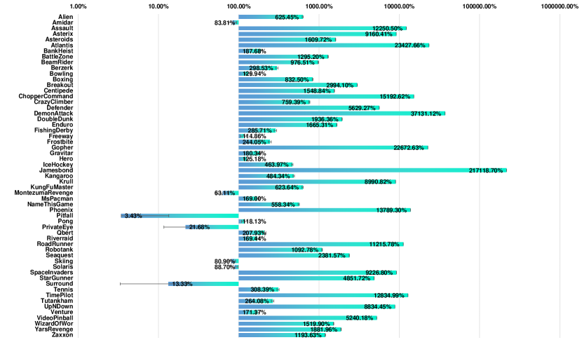
Figure 12: HNS (%) of Atari 57 games using GDI-I³.

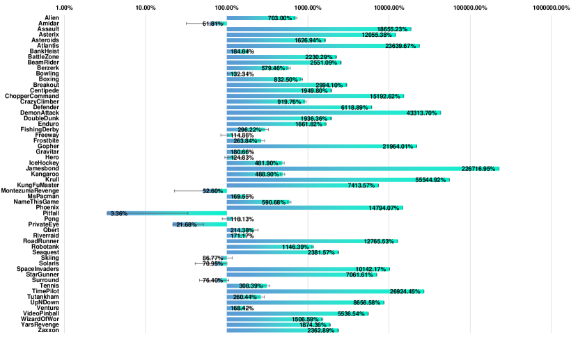
Figure 13: HNS (%) of Atari 57 games using GDI-H³.

J.3 Figure of HWRNS

In this part, we begin to visualize the HWRNS (Hafner et al., 2020; Toromanoff et al., 2019) using GDI-H³ and GDI-I³ in all 57 games. The HWRNS histogram of GDI-I³ is illustrated in Fig. 14. The HWRNS histogram of GDI-H³ is illustrated in Fig. 15. In addition, we mark the error bars in the histogram with respect to the random seed after running experiments multiple times.

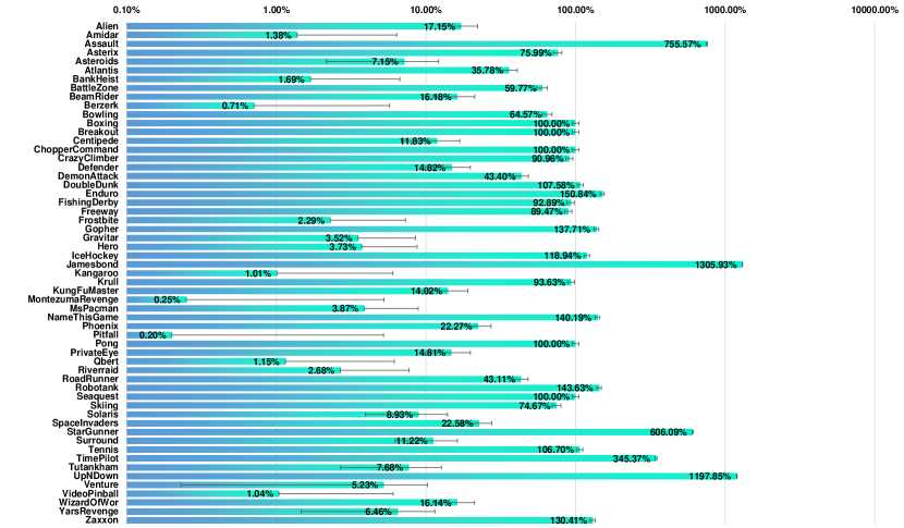
Figure 14: HWRNS (%) of Atari 57 games using GDI-I³.

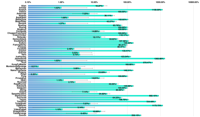
Figure 15: HWRNS (%) of Atari 57 games using GDI-H³.

J.4 Figure of SABER

In this part, we begin to visualize the HWRNS (Hafner et al., 2020; Toromanoff et al., 2019) using GDI-H³ and GDI-I³ in all 57 games. The HWRNS histogram of GDI-I³ is illustrated in Fig. 16. The HWRNS histogram of GDI-H³ is illustrated in Fig. 17. In addition, we mark the error bars in the histogram with respect to the random seed after running experiments multiple times.

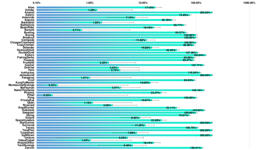
Figure 16: SABER (%) of Atari 57 games using GDI-I³.

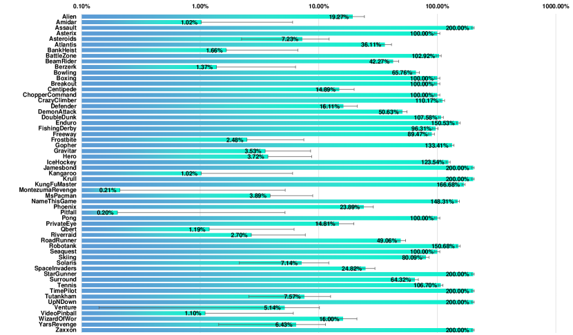
Figure 17: SABER (%) of Atari 57 games using GDI-H³.

J.5 Atari Games Table of Scores Based on Human Average Records

In this part, we detail the raw score of several representative SOTA algorithms including the SOTA 200M model-free algorithms, SOTA 10B+ model-free algorithms, SOTA model-based algorithms and other SOTA algorithms.

Additionally, we calculate the Human Normalized Score (HNS) of each game with each algorithms. First of all, we demonstrate the sources of the scores that we used. Random scores and average human’s scores are from (Badia et al., 2020a). Rainbow’s scores are from (Hessel et al., 2017). IMPALA’s scores are from (Espeholt et al., 2018). LASER’s scores are from (Schmitt et al., 2020), no sweep at 200M. As there are many versions of R2D2 and NGU, we use original papers’. R2D2’s scores are from (Kapturowski et al., 2018). NGU’s scores are from (Badia et al., 2020b). Agent57’s scores are from (Badia et al., 2020a). MuZero’s scores are from (Schrittwieser et al., 2020). DreamerV2’s scores are from (Hafner et al., 2020). SimPLe’s scores are form (Kaiser et al., 2019). Go-Explore’s scores are form (Ecoffet et al., 2019). Muesli’s scores are form (Hessel et al., 2021). In the following we detail the raw scores and HNS of each algorithms on 57 Atari games.

J.5.1 Comparison with SOTA 200M Model-Free Algorithms on HNS

Games	RND	HUMAN	RAINBOW	HNS(%)	IMPALA	HNS(%)	LASER	HNS(%)	GDI-I3	HNS(%)	GDI-H3	HNS(%)
Scale			200M		200M		200M		200M		200M
alien	227.8	7127.8	9491.7	134.26	15962.1	228.03	35565.9	512.15	43384	625.45	48735	703.00
amidar	5.8	1719.5	5131.2	299.08	1554.79	90.39	1829.2	106.4	1442	83.81	1065	61.81
assault	222.4	742	14198.5	2689.78	19148.47	3642.43	21560.4	4106.62	63876	12250.50	97155	18655.23
asterix	210	8503.3	428200	5160.67	300732	3623.67	240090	2892.46	759910	9160.41	999999	12055.38
asteroids	719	47388.7	2712.8	4.27	108590.05	231.14	213025	454.91	751970	1609.72	760005	1626.94
atlantis	12850	29028.1	826660	5030.32	849967.5	5174.39	841200	5120.19	3803000	23427.66	3837300	23639.67
bank heist	14.2	753.1	1358	181.86	1223.15	163.61	569.4	75.14	1401	187.68	1380	184.84
battle zone	236	37187.5	62010	167.18	20885	55.88	64953.3	175.14	478830	1295.20	824360	2230.29
beam rider	363.9	16926.5	16850.2	99.54	32463.47	193.81	90881.6	546.52	162100	976.51	422890	2551.09
berzerk	123.7	2630.4	2545.6	96.62	1852.7	68.98	25579.5	1015.51	7607	298.53	14649	579.46
bowling	23.1	160.7	30	5.01	59.92	26.76	48.3	18.31	201.9	129.94	205.2	132.34
boxing	0.1	12.1	99.6	829.17	99.96	832.17	100	832.5	100	832.50	100	832.50
breakout	1.7	30.5	417.5	1443.75	787.34	2727.92	747.9	2590.97	864	2994.10	864	2994.10
centipede	2090.9	12017	8167.3	61.22	11049.75	90.26	292792	2928.65	155830	1548.84	195630	1949.80
chopper command	811	7387.8	16654	240.89	28255	417.29	761699	11569.27	999999	15192.62	999999	15192.62
crazy climber	10780.5	36829.4	168788.5	630.80	136950	503.69	167820	626.93	201000	759.39	241170	919.76
defender	2874.5	18688.9	55105	330.27	185203	1152.93	336953	2112.50	893110	5629.27	970540	6118.89
demon attack	152.1	1971	111185	6104.40	132826.98	7294.24	133530	7332.89	675530	37131.12	787985	43313.70
double dunk	-18.6	-16.4	-0.3	831.82	-0.33	830.45	14	1481.82	24	1936.36	24	1936.36
enduro	0	860.5	2125.9	247.05	0	0.00	0	0.00	14330	1665.31	14300	1661.82
fishing derby	-91.7	-38.8	31.3	232.51	44.85	258.13	45.2	258.79	59	285.71	65	296.22
freeway	0	29.6	34	114.86	0	0.00	0	0.00	34	114.86	34	114.86
frostbite	65.2	4334.7	9590.5	223.10	317.75	5.92	5083.5	117.54	10485	244.05	11330	263.84
gopher	257.6	2412.5	70354.6	3252.91	66782.3	3087.14	114820.7	5316.40	488830	22672.63	473560	21964.01
gravitar	173	3351.4	1419.3	39.21	359.5	5.87	1106.2	29.36	5905	180.34	5915	180.66
hero	1027	30826.4	55887.4	184.10	33730.55	109.75	31628.7	102.69	38330	125.18	38225	124.83
ice hockey	-11.2	0.9	1.1	101.65	3.48	121.32	17.4	236.36	44.94	463.97	47.11	481.90
jamesbond	29	302.8	19809	72.24	601.5	209.09	37999.8	13868.08	594500	217118.70	620780	226716.95
kangaroo	52	3035	14637.5	488.05	1632	52.97	14308	477.91	14500	484.34	14636	488.00
krull	1598	2665.5	8741.5	669.18	8147.4	613.53	9387.5	729.70	97575	8990.82	594540	55544.92
kung fu master	258.5	22736.3	52181	230.99	43375.5	191.82	607443	2701.26	140440	623.64	1666665	7413.57
montezuma revenge	0	4753.3	384	8.08	0	0.00	0.3	0.01	3000	63.11	2500	52.60
ms pacman	307.3	6951.6	5380.4	76.35	7342.32	105.88	6565.5	94.19	11536	169.00	11573	169.55
name this game	2292.3	8049	13136	188.37	21537.2	334.30	26219.5	415.64	34434	558.34	36296	590.68
phoenix	761.5	7242.6	108529	1662.80	210996.45	3243.82	519304	8000.84	894460	13789.30	959580	14794.07
pitfall	-229.4	6463.7	0	3.43	-1.66	3.40	-0.6	3.42	0	3.43	-4.345	3.36
pong	-20.7	14.6	20.9	117.85	20.98	118.07	21	118.13	21	118.13	21	118.13
private eye	24.9	69571.3	4234	6.05	98.5	0.11	96.3	0.10	15100	21.68	15100	21.68
qbert	163.9	13455.0	33817.5	253.20	351200.12	2641.14	21449.6	160.15	27800	207.93	28657	214.38
riverraid	1338.5	17118.0	22920.8	136.77	29608.05	179.15	40362.7	247.31	28075	169.44	28349	171.17
road runner	11.5	7845	62041	791.85	57121	729.04	45289	578.00	878600	11215.78	999999	12765.53
robotank	2.2	11.9	61.4	610.31	12.96	110.93	62.1	617.53	108.2	1092.78	113.4	1146.39
seaquest	68.4	42054.7	15898.9	37.70	1753.2	4.01	2890.3	6.72	943910	2247.98	1000000	2381.57
skiing	-17098	-4336.9	-12957.8	32.44	-10180.38	54.21	-29968.4	-100.86	-6774	80.90	-6025	86.77
solaris	1236.3	12326.7	3560.3	20.96	2365	10.18	2273.5	9.35	11074	88.70	9105	70.95
space invaders	148	1668.7	18789	1225.82	43595.78	2857.09	51037.4	3346.45	140460	9226.80	154380	10142.17
star gunner	664	10250	127029	1318.22	200625	2085.97	321528	3347.21	465750	4851.72	677590	7061.61
surround	-10	6.5	9.7	119.39	7.56	106.42	8.4	111.52	-7.8	13.33	2.606	76.40
tennis	-23.8	-8.3	0	153.55	0.55	157.10	12.2	232.26	24	308.39	24	308.39
time pilot	3568	5229.2	12926	563.36	48481.5	2703.84	105316	6125.34	216770	12834.99	450810	26924.45
tutankham	11.4	167.6	241	146.99	292.11	179.71	278.9	171.25	423.9	264.08	418.2	260.44
up n down	533.4	11693.2	125755	1122.08	332546.75	2975.08	345727	3093.19	986440	8834.45	966590	8656.58
venture	0	1187.5	5.5	0.46	0	0.00	0	0.00	2035	171.37	2000	168.42
video pinball	0	17667.9	533936.5	3022.07	572898.27	3242.59	511835	2896.98	925830	5240.18	978190	5536.54
wizard of wor	563.5	4756.5	17862.5	412.57	9157.5	204.96	29059.3	679.60	64239	1519.90	63735	1506.59
yars revenge	3092.9	54576.9	102557	193.19	84231.14	157.60	166292.3	316.99	972000	1881.96	968090	1874.36
zaxxon	32.5	9173.3	22209.5	242.62	32935.5	359.96	41118	449.47	109140	1193.63	216020	2362.89
MEAN HNS(%)	0.00	100.00		873.97		957.34		1741.36		7810.6		9620.98
Learning Efficiency	0.00	N/A		4.37E-08		4.79E-08		8.71E-08		3.91E-07		4.70E-07
MEDIAN HNS(%)	0.00	100.00		230.99		191.82		454.91		832.5		1146.39
Learning Efficiency	0.00	N/A		1.15E-08		9.59E-09		2.27E-08		4.16E-08		5.73E-08

Table 8: Score table of SOTA 200M model-free algorithms on HNS.

J.5.2 Comparison with SOTA 10B+ model-free algorithms on HNS

Games	R2D2	HNS(%)	NGU	HNS(%)	AGENT57	HNS(%)	GDI-I3	HNS(%)	GDI-H3	HNS(%)
Scale	10B		35B		100B		200M		200M
alien	109038.4	1576.97	248100	3592.35	297638.17	4310.30	43384	625.45	48735	703.00
amidar	27751.24	1619.04	17800	1038.35	29660.08	1730.42	1442	83.81	1065	61.81
assault	90526.44	17379.53	34800	6654.66	67212.67	12892.66	63876	12250.50	97155	18655.23
asterix	999080	12044.30	950700	11460.94	991384.42	11951.51	759910	9160.41	999999	12055.38
asteroids	265861.2	568.12	230500	492.36	150854.61	321.70	751970	1609.72	760005	1626.94
atlantis	1576068	9662.56	1653600	10141.80	1528841.76	9370.64	3803000	23427.66	3837300	23639.67
bank heist	46285.6	6262.20	17400	2352.93	23071.5	3120.49	1401	187.68	1380	184.84
battle zone	513360	1388.64	691700	1871.27	934134.88	2527.36	478830	1295.20	824360	2230.29
beam rider	128236.08	772.05	63600	381.80	300509.8	1812.19	162100	976.51	422390	2548.07
berzerk	34134.8	1356.81	36200	1439.19	61507.83	2448.80	7607	298.53	14649	579.46
bowling	196.36	125.92	211.9	137.21	251.18	165.76	201.9	129.94	205.2	132.34
boxing	99.16	825.50	99.7	830.00	100	832.50	100	832.50	100	832.50
breakout	795.36	2755.76	559.2	1935.76	790.4	2738.54	864	2994.10	864	2994.10
centipede	532921.84	5347.83	577800	5799.95	412847.86	4138.15	155830	1548.84	195630	1949.80
chopper command	960648	14594.29	999900	15191.11	999900	15191.11	999999	15192.62	999999	15192.62
crazy climber	312768	1205.59	313400	1208.11	565909.85	2216.18	201000	759.39	241170	919.76
defender	562106	3536.22	664100	4181.16	677642.78	4266.80	893110	5629.27	970540	6118.89
demon attack	143664.6	7890.07	143500	7881.02	143161.44	7862.41	675530	37131.12	787985	43313.70
double dunk	23.12	1896.36	-14.1	204.55	23.93	1933.18	24	1936.36	24	1936.36
enduro	2376.68	276.20	2000	232.42	2367.71	275.16	14330	1665.31	14300	1661.82
fishing derby	81.96	328.28	32	233.84	86.97	337.75	59	285.71	65	296.22
freeway	34	114.86	28.5	96.28	32.59	110.10	34	114.86	34	114.86
frostbite	11238.4	261.70	206400	4832.76	541280.88	12676.32	10485	244.05	11330	263.84
gopher	122196	5658.66	113400	5250.47	117777.08	5453.59	488830	22672.63	473560	21964.01
gravitar	6750	206.93	14200	441/32	19213.96	599.07	5905	180.34	5915	180.66
hero	37030.4	120.82	69400	229.44	114736.26	381.58	38330	125.18	38225	124.83
ice hockey	71.56	683.97	-4.1	58.68	63.64	618.51	44.94	463.97	47.11	481.90
jamesbond	23266	8486.85	26600	9704.53	135784.96	49582.16	594500	217118.70	620780	226716.95
kangaroo	14112	471.34	35100	1174.92	24034.16	803.96	14500	484.34	14636	488.90
krull	145284.8	13460.12	127400	11784.73	251997.31	23456.61	97575	8990.82	594540	55544.92
kung fu master	200176	889.40	212100	942.45	206845.82	919.07	140440	623.64	1666665	7413.57
montezuma revenge	2504	52.68	10400	218.80	9352.01	196.75	3000	63.11	2500	52.60
ms pacman	29928.2	445.81	40800	609.44	63994.44	958.52	11536	169.00	11573	169.55
name this game	45214.8	745.61	23900	375.35	54386.77	904.94	34434	558.34	36296	590.68
phoenix	811621.6	125.11	959100	14786.66	908264.15	14002.29	894460	13789.30	959580	14794.07
pitfall	0	3.43	7800	119.97	18756.01	283.66	0	3.43	-4.3	3.36
pong	21	118.13	19.6	114.16	20.67	117.20	21	118.13	21	118.13
private eye	300	0.40	100000	143.75	79716.46	114.59	15100	21.68	15100	21.68
qbert	161000	1210.10	451900	3398.79	580328.14	4365.06	27800	207.93	28657	214.38
riverraid	34076.4	207.47	36700	224.10	63318.67	392.79	28075	169.44	28349	171.17
road runner	498660	6365.59	128600	1641.52	243025.8	3102.24	878600	11215.78	999999	12765.53
robotank	132.4	1342.27	9.1	71.13	127.32	1289.90	108.2	1092.78	113.4	1146.39
seaquest	999991.84	2381.55	1000000	2381.57	999997.63	2381.56	943910	2247.98	1000000	2381.57
skiing	-29970.32	-100.87	-22977.9	-46.08	-4202.6	101.05	-6774	80.90	-6025	86.77
solaris	4198.4	26.71	4700	31.23	44199.93	387.39	11074	88.70	9105	70.95
space invaders	55889	3665.48	43400	2844.22	48680.86	3191.48	140460	9226.80	154380	10142.17
star gunner	521728	5435.68	414600	4318.13	839573.53	8751.40	465750	4851.72	677590	7061.61
surround	9.96	120.97	-9.6	2.42	9.5	118.18	-7.8	13.33	2.606	76.40
tennis	24	308.39	10.2	219.35	23.84	307.35	24	308.39	24	308.39
time pilot	348932	20791.28	344700	20536.51	405425.31	24192.24	216770	12834.99	450810	26924.45
tutankham	393.64	244.71	191.1	115.04	2354.91	1500.33	423.9	264.08	418.2	260.44
up n down	542918.8	4860.17	620100	5551.77	623805.73	5584.98	986440	8834.45	966590	8656.58
venture	1992	167.75	1700	143.16	2623.71	220.94	2035	171.37	2000	168.42
video pinball	483569.72	2737.00	965300	5463.58	992340.74	5616.63	925830	5240.18	978190	5536.54
wizard of wor	133264	3164.81	106200	2519.35	157306.41	3738.20	64293	1519.90	63735	1506.59
yars revenge	918854.32	1778.73	986000	1909.15	998532.37	1933.49	972000	1881.96	968090	1874.36
zaxxon	181372	1983.85	111100	1215.07	249808.9	2732.54	109140	1193.63	216020	2362.89
MEAN HNS(%)		3374.31		3169.90		4763.69		7810.6		9620.98
Learning Efficiency		3.37E-09		9.06E-10		4.76E-10		3.91E-07		4.81E-07
MEDIAN HNS(%)		1342.27		1208.11		1933.49		832.5		1146.39
Learning Efficiency		1.34E-09		3.45E-10		1.93E-10		4.16E-08		5.73E-08

Table 9: Score table of SOTA model-free algorithms on HNS.

J.5.3 Comparison with SOTA Model-Based Algorithms on HNS

SimPLe (Kaiser et al., 2019) and DreamerV2(Hafner et al., 2020) haven’t evaluated all 57 Atari Games in their paper. For fairness, we set the score on those games as N/A, which will not be considered when calculating the median and mean HNS.

Games	MuZero	HNS(%)	DreamerV2	HNS(%)	SimPLe	HNS(%)	GDI-I3	HNS(%)	GDI-H3	HNS(%)
Scale	20B		200M		1M		200M		200M
alien	741812.63	10747.61	3483	47.18	616.9	5.64	43384	625.45	48735	703.00
amidar	28634.39	1670.57	2028	118.00	74.3	4.00	1442	83.81	1065	61.81
assault	143972.03	27665.44	7679	1435.07	527.2	58.66	63876	12250.50	97155	18655.23
asterix	998425	12036.40	25669	306.98	1128.3	11.07	759910	9160.41	999999	12055.38
asteroids	678558.64	1452.42	3064	5.02	793.6	0.16	751970	1609.72	760005	1626.94
atlantis	1674767.2	10272.64	989207	6035.05	20992.5	50.33	3803000	23427.66	3837300	23639.67
bank heist	1278.98	171.17	1043	139.23	34.2	2.71	1401	187.68	1380	184.84
battle zone	848623	2295.95	31225	83.86	4031.2	10.27	478830	1295.20	824360	2230.29
beam rider	454993.53	2744.92	12413	72.75	621.6	1.56	162100	976.51	422390	2548.07
berzerk	85932.6	3423.18	751	25.02	N/A	N/A	7607	298.53	14649	579.46
bowling	260.13	172.26	48	18.10	30	5.01	202	129.94	205.2	132.34
boxing	100	832.50	87	724.17	7.8	64.17	100	832.50	100	832.50
breakout	864	2994.10	350	1209.38	16.4	51.04	864	2994.10	864	2994.10
centipede	1159049.27	11655.72	6601	45.44	N/A	N/A	155830	1548.84	195630	1949.80
chopper command	991039.7	15056.39	2833	30.74	979.4	2.56	999999	15192.62	999999	15192.62
crazy climber	458315.4	1786.64	141424	521.55	62583.6	206.81	201000	759.39	241170	919.76
defender	839642.95	5291.18	N/A	N/A	N/A	N/A	893110	5629.27	970540	6118.89
demon attack	143964.26	7906.55	2775	144.20	208.1	3.08	675530	37131.12	787985	43313.70
double dunk	23.94	1933.64	22	1845.45	N/A	N/A	24	1936.36	24	1936.36
enduro	2382.44	276.87	2112	245.44	N/A	N/A	14330	1665.31	14300	1661.82
fishing derby	91.16	345.67	60	286.77	-90.7	1.89	59	285.71	65	296.22
freeway	33.03	111.59	34	114.86	16.7	56.42	34	114.86	34	114.86
frostbite	631378.53	14786.59	15622	364.37	236.9	4.02	10485	244.05	11330	263.84
gopher	130345.58	6036.85	53853	2487.14	596.8	15.74	488830	22672.6	473560	21964.01
gravitar	6682.7	204.81	3554	106.37	173.4	0.01	5905	180.34	5915	180.66
hero	49244.11	161.81	30287	98.19	2656.6	5.47	38330	125.18	38225	124.83
ice hockey	67.04	646.61	29	332.23	-11.6	-3.31	44.94	463.97	47.11	481.90
jamesbond	41063.25	14986.94	9269	3374.73	100.5	26.11	594500	217118.70	620780	226716.95
kangaroo	16763.6	560.23	11819	394.47	51.2	-0.03	14500	484.34	14636	488.90
krull	269358.27	25082.93	9687	757.75	2204.8	56.84	97575	8990.82	594540	55544.92
kung fu master	204824	910.08	66410	294.30	14862.5	64.97	140440	623.64	1666665	7413.57
montezuma revenge	0	0.00	1932	40.65	N/A	N/A	3000	63.11	2500	52.60
ms pacman	243401.1	3658.68	5651	80.43	1480	17.65	11536	169.00	11573	169.55
name this game	157177.85	2690.53	14472	211.57	2420.7	2.23	34434	558.34	36296	590.68
phoenix	955137.84	14725.53	13342	194.11	N/A	N/A	894460	13789.30	959580	14794.07
pitfall	0	3.43	-1	3.41	N/A	N/A	0	3.43	-4.3	3.36
pong	21	118.13	19	112.46	12.8	94.90	21	118.13	21	118.13
private eye	15299.98	21.96	158	0.19	35	0.01	15100	21.68	15100	21.68
qbert	72276	542.56	162023	1217.80	1288.8	8.46	27800	207.93	28657	214.38
riverraid	323417.18	2041.12	16249	94.49	1957.8	3.92	28075	169.44	28349	171.17
road runner	613411.8	7830.48	88772	1133.09	5640.6	71.86	878600	11215.78	999999	12765.53
robotank	131.13	1329.18	65	647.42	N/A	N/A	108	1092.78	113.4	1146.39
seaquest	999976.52	2381.51	45898	109.15	683.3	1.46	943910	2247.98	1000000	2381.57
skiing	-29968.36	-100.86	-8187	69.83	N/A	N/A	-6774	80.90	-6025	86.77
solaris	56.62	-10.64	883	-3.19	N/A	N/A	11074	88.70	9105	70.95
space invaders	74335.3	4878.50	2611	161.96	N/A	N/A	140460	9226.80	154380	10142.17
star gunner	549271.7	5723.01	29219	297.88	N/A	N/A	465750	4851.72	677590	7061.61
surround	9.99	121.15	N/A	N/A	N/A	N/A	-7.8	13.33	2.606	76.40
tennis	0	153.55	23	301.94	N/A	N/A	24	308.39	24	308.39
time pilot	476763.9	28486.90	32404	1735.96	N/A	N/A	216770	12834.99	450810	26924.45
tutankham	491.48	307.35	238	145.07	N/A	N/A	424	264.08	418.2	260.44
up n down	715545.61	6407.03	648363	5805.03	3350.3	25.24	986440	8834.45	966590	8656.58
venture	0.4	0.03	0	0.00	N/A	N/A	2035	171.37	2000	168.42
video pinball	981791.88	5556.92	22218	125.75	N/A	N/A	925830	5240.18	978190	5536.54
wizard of wor	197126	4687.87	14531	333.11	N/A	N/A	64439	1523.38	63735	1506.59
yars revenge	553311.46	1068.72	20089	33.01	5664.3	4.99	972000	1881.96	968090	1874.36
zaxxon	725853.9	7940.46	18295	199.79	N/A	N/A	109140	1193.63	216020	2362.89
MEAN HNS(%)		4996.20		631.17		25.3		7810.6		9620.98
Learning Efficiency		2.50E-09		3.16E-08		2.53E-07		3.91E-07		4.81E-07
MEDIAN HNS(%)		2041.12		161.96		5.55		832.5		1146.39
Learning Efficiency		1.02E-09		8.10E-09		5.55E-08		4.16E-08		5.73E-08

Table 10: Score table of SOTA model-based algorithms on HNS.

J.5.4 Comparison with Other SOTA algorithms on HNS

In this section, we report the performance of our algorithm compared with other SOTA algorithms, Go-Explore (Ecoffet et al., 2019) and Muesli (Hessel et al., 2021).

Games	Muesli	HNS(%)	Go-Explore	HNS(%)	GDI-I3	HNS(%)	GDI-H3	HNS(%)
Scale	200M		10B		200M		200M
alien	139409	2017.12	959312	13899.77	43384	625.45	48735	703.00
amidar	21653	1263.18	19083	1113.22	1442	83.81	1065	61.81
assault	36963	7070.94	30773	5879.64	63876	12250.50	97155	18655.23
asterix	316210	3810.30	999500	12049.37	759910	9160.41	999999	12055.38
asteroids	484609	1036.84	112952	240.48	751970	1609.72	760005	1626.94
atlantis	1363427	8348.18	286460	1691.24	3803000	23427.66	3837300	23639.67
bank heist	1213	162.24	3668	494.49	1401	187.68	1380	184.84
battle zone	414107	1120.04	998800	2702.36	478830	1295.20	824360	2230.29
beam rider	288870	1741.91	371723	2242.15	162100	976.51	422390	2548.07
berzerk	44478	1769.43	131417	5237.69	7607	298.53	14649	579.46
bowling	191	122.02	247	162.72	202	129.94	205.2	132.34
boxing	99	824.17	91	757.50	100	832.50	100	832.50
breakout	791	2740.63	774	2681.60	864	2994.10	864	2994.10
centipede	869751	8741.20	613815	6162.78	155830	1548.84	195630	1949.80
chopper command	101289	1527.76	996220	15135.16	999999	15192.62	999999	15192.62
crazy climber	175322	656.88	235600	897.52	201000	759.39	241170	919.76
defender	629482	3962.26	N/A	N/A	893110	5629.27	970540	6118.89
demon attack	129544	7113.74	239895	13180.65	675530	37131.12	787985	43313.70
double dunk	-3	709.09	24	1936.36	24	1936.36	24	1936.36
enduro	2362	274.49	1031	119.81	14330	1665.31	14300	1661.82
fishing derby	51	269.75	67	300.00	59	285.71	65	296.22
freeway	33	111.49	34	114.86	34	114.86	34	114.86
frostbite	301694	7064.73	999990	23420.19	10485	244.05	11330	263.84
gopher	104441	4834.72	134244	6217.75	488830	22672.63	473560	21964.01
gravitar	11660	361.41	13385	415.68	5905	180.34	5915	180.66
hero	37161	121.26	37783	123.34	38330	125.18	38225	124.83
ice hockey	25	299.17	33	365.29	44.94	463.97	47.11	481.90
jamesbond	19319	7045.29	200810	73331.26	594500	217118.70	620780	226716.95
kangaroo	14096	470.80	24300	812.87	14500	484.34	14636	488.90
krull	34221	3056.02	63149	5765.90	97575	8990.82	594540	55544.92
kung fu master	134689	598.06	24320	107.05	140440	623.64	1666665	7413.57
montezuma revenge	2359	49.63	24758	520.86	3000	63.11	2500	52.60
ms pacman	65278	977.84	456123	6860.25	11536	169.00	11573	169.55
name this game	105043	1784.89	212824	3657.16	34434	558.34	36296	590.68
phoenix	805305	12413.69	19200	284.50	894460	13789.30	959580	14794.07
pitfall	0	3.43	7875	121.09	0	3.43	-4.3	3.36
pong	20	115.30	21	118.13	21	118.13	21	118.13
private eye	10323	14.81	69976	100.58	15100	21.68	15100	21.68
qbert	157353	1182.66	999975	7522.41	27800	207.93	28657	214.38
riverraid	47323	291.42	35588	217.05	28075	169.44	28349	171.17
road runner	327025	4174.55	999900	12764.26	878600	11215.78	999999	12765.53
robotank	59	585.57	143	1451.55	108	1092.78	113.4	1146.39
seaquest	815970	1943.26	539456	1284.68	943910	2247.98	1000000	2381.57
skiing	-18407	-10.26	-4185	101.19	-6774	80.90	-6025	86.77
solaris	3031	16.18	20306	171.95	11074	88.70	9105	70.95
space invaders	59602	3909.65	93147	6115.54	140460	9226.80	154380	10142.17
star gunner	214383	2229.49	609580	6352.14	465750	4851.72	677590	7061.61
surround	9	115.15	N/A	N/A	-8	13.33	2.606	76.40
tennis	12	230.97	24	308.39	24	308.39	24	308.39
time pilot	359105	21403.71	183620	10839.32	216770	12834.99	450810	26924.45
tutankham	252	154.03	528	330.73	424	264.08	418.2	260.44
up n down	649190	5812.44	553718	4956.94	986440	8834.45	966590	8656.58
venture	2104	177.18	3074	258.86	2035	171.37	2000	168.42
video pinball	685436	3879.56	999999	5659.98	925830	5240.18	978190	5536.54
wizard of wor	93291	2211.48	199900	4754.03	64293	1519.90	63735	1506.59
yars revenge	557818	1077.47	999998	1936.34	972000	1881.96	968090	1874.36
zaxxon	65325	714.30	18340	200.28	109140	1193.63	216020	2362.89
MEAN HNS(%)		2538.66		4989.94		7810.6		9620.98
Learning Efficiency		1.27E-07		4.99E-09		3.91E-07		4.81E-07
MEDIAN HNS(%)		1077.47		1451.55		832.5		1146.39
Learning Efficiency		5.39E-08		1.45E-09		4.16E-08		5.73E-08

Table 11: Score table of other SOTA algorithms on HNS.

J.6 Atari Games Table of Scores Based on Human World Records

In this part, we detail the raw score of several representative SOTA algorithms including the SOTA 200M model-free algorithms, SOTA 10B+ model-free algorithms, SOTA model-based algorithms and other SOTA algorithms.

Additionally, we calculate the human world records normalized world score (HWRNS) of each game with each algorithms. First of all, we demonstrate the sources of the scores that we used. Random scores are from (Badia et al., 2020a). Human world records (HWR) are form (Hafner et al., 2020; Toromanoff et al., 2019). Rainbow’s scores are from (Hessel et al., 2017). IMPALA’s scores are from (Espeholt et al., 2018). LASER’s scores are from (Schmitt et al., 2020), no sweep at 200M. As there are many versions of R2D2 and NGU, we use original papers’. R2D2’s scores are from (Kapturowski et al., 2018). NGU’s scores are from (Badia et al., 2020b). Agent57’s scores are from (Badia et al., 2020a). MuZero’s scores are from (Schrittwieser et al., 2020). DreamerV2’s scores are from (Hafner et al., 2020). SimPLe’s scores are form (Kaiser et al., 2019). Go-Explore’s scores are form (Ecoffet et al., 2019). Muesli’s scores are form (Hessel et al., 2021). In the following we detail the raw scores and HWRNS of each algorithms on 57 Atari games.

J.6.1 Comparison with SOTA 200M Algorithms on HWRNS

Games	RND	HWR	RAINBOW	HWRNS(%)	IMPALA	HWRNS(%)	LASER	HWRNS(%)	GDI-I3	HWRNS(%)	GDI-H3	HWRNS(%)
Scale			200M		200M		200M		200M		200M
alien	227.8	251916	9491.7	3.68	15962.1	6.25	976.51	14.04	43384	17.15	48735	19.27
amidar	5.8	104159	5131.2	4.92	1554.79	1.49	1829.2	1.75	1442	1.38	1065	1.02
assault	222.4	8647	14198.5	165.90	19148.47	224.65	21560.4	253.28	63876	755.57	97155	1150.59
asterix	210	1000000	428200	42.81	300732	30.06	240090	23.99	759910	75.99	999999	100.00
asteroids	719	10506650	2712.8	0.02	108590.05	1.03	213025	2.02	751970	7.15	760005	7.23
atlantis	12850	10604840	826660	7.68	849967.5	7.90	841200	7.82	3803000	35.78	3837300	36.11
bank heist	14.2	82058	1358	1.64	1223.15	1.47	569.4	0.68	1401	1.69	1380	1.66
battle zone	236	801000	62010	7.71	20885	2.58	64953.3	8.08	478830	59.77	824360	102.92
beam rider	363.9	999999	16850.2	1.65	32463.47	3.21	90881.6	9.06	162100	16.18	422390	42.22
berzerk	123.7	1057940	2545.6	0.23	1852.7	0.16	25579.5	2.41	7607	0.71	14649	1.37
bowling	23.1	300	30	2.49	59.92	13.30	48.3	9.10	201.9	64.57	205.2	65.76
boxing	0.1	100	99.6	99.60	99.96	99.96	100	100.00	100	100.00	100	100.00
breakout	1.7	864	417.5	48.22	787.34	91.11	747.9	86.54	864	100.00	864	100.00
centipede	2090.9	1301709	8167.3	0.47	11049.75	0.69	292792	22.37	155830	11.83	195630	14.89
chopper command	811	999999	16654	1.59	28255	2.75	761699	76.15	999999	100.00	999999	100.00
crazy climber	10780.5	219900	168788.5	75.56	136950	60.33	167820	75.10	201000	90.96	241170	110.17
defender	2874.5	6010500	55105	0.87	185203	3.03	336953	5.56	893110	14.82	970540	16.11
demon attack	152.1	1556345	111185	7.13	132826.98	8.53	133530	8.57	675530	43.40	787985	50.63
double dunk	-18.6	21	-0.3	46.21	-0.33	46.14	14	82.32	24	107.58	24	107.58
enduro	0	9500	2125.9	22.38	0	0.00	0	0.00	14330	150.84	14300	150.53
fishing derby	-91.7	71	31.3	75.60	44.85	83.93	45.2	84.14	59	92.89	65	96.31
freeway	0	38	34	89.47	0	0.00	0	0.00	34	89.47	34	89.47
frostbite	65.2	454830	9590.5	2.09	317.75	0.06	5083.5	1.10	10485	2.29	11330	2.48
gopher	257.6	355040	70354.6	19.76	66782.3	18.75	114820.7	32.29	488830	137.71	473560	133.41
gravitar	173	162850	1419.3	0.77	359.5	0.11	1106.2	0.57	5905	3.52	5915	3.53
hero	1027	1000000	55887.4	5.49	33730.55	3.27	31628.7	3.06	38330	3.73	38225	3.72
ice hockey	-11.2	36	1.1	26.06	3.48	31.10	17.4	60.59	44.92	118.94	47.11	123.54
jamesbond	29	45550	19809	43.45	601.5	1.26	37999.8	83.41	594500	1305.93	620780	1363.66
kangaroo	52	1424600	14637.5	1.02	1632	0.11	14308	1.00	14500	1.01	14636	1.02
krull	1598	104100	8741.5	6.97	8147.4	6.39	9387.5	7.60	97575	93.63	594540	578.47
kung fu master	258.5	1000000	52181	5.19	43375.5	4.31	607443	60.73	140440	14.02	1666665	166.68
montezuma revenge	0	1219200	384	0.03	0	0.00	0.3	0.00	3000	0.25	2500	0.21
ms pacman	307.3	290090	5380.4	1.75	7342.32	2.43	6565.5	2.16	11536	3.87	11573	3.89
name this game	2292.3	25220	13136	47.30	21537.2	83.94	26219.5	104.36	34434	140.19	36296	148.31
phoenix	761.5	4014440	108529	2.69	210996.45	5.24	519304	12.92	894460	22.27	959580	23.89
pitfall	-229.4	114000	0	0.20	-1.66	0.20	-0.6	0.20	0	0.20	-4.3	0.20
pong	-20.7	21	20.9	99.76	20.98	99.95	21	100.00	21	100.00	21	100.00
private eye	24.9	101800	4234	4.14	98.5	0.07	96.3	0.07	15100	14.81	15100	14.81
qbert	163.9	2400000	33817.5	1.40	351200.12	14.63	21449.6	0.89	27800	1.15	28657	1.19
riverraid	1338.5	1000000	22920.8	2.16	29608.05	2.83	40362.7	3.91	28075	2.68	28349	2.70
road runner	11.5	2038100	62041	3.04	57121	2.80	45289	2.22	878600	43.11	999999	49.06
robotank	2.2	76	61.4	80.22	12.96	14.58	62.1	81.17	108.2	143.63	113.4	150.68
seaquest	68.4	999999	15898.9	1.58	1753.2	0.17	2890.3	0.28	943910	94.39	1000000	100.00
skiing	-17098	-3272	-12957.8	29.95	-10180.38	50.03	-29968.4	-93.09	-6774	74.67	-6025	86.77
solaris	1236.3	111420	3560.3	2.11	2365	1.02	2273.5	0.94	11074	8.93	9105	7.14
space invaders	148	621535	18789	3.00	43595.78	6.99	51037.4	8.19	140460	22.58	154380	24.82
star gunner	664	77400	127029	164.67	200625	260.58	321528	418.14	465750	606.09	677590	882.15
surround	-10	9.6	9.7	100.51	7.56	89.59	8.4	93.88	-7.8	11.22	2.606	64.32
tennis	-23.8	21	0	53.13	0.55	54.35	12.2	80.36	24	106.70	24	106.70
time pilot	3568	65300	12926	15.16	48481.5	72.76	105316	164.82	216770	345.37	450810	724.49
tutankham	11.4	5384	241	4.27	292.11	5.22	278.9	4.98	423.9	7.68	418.2	7.57
up n down	533.4	82840	125755	152.14	332546.75	403.39	345727	419.40	986440	1197.85	966590	1173.73
venture	0	38900	5.5	0.01	0	0.00	0	0.00	2000	5.23	2000	5.14
video pinball	0	89218328	533936.5	0.60	572898.27	0.64	511835	0.57	925830	1.04	978190	1.10
wizard of wor	563.5	395300	17862.5	4.38	9157.5	2.18	29059.3	7.22	64439	16.14	63735	16.00
yars revenge	3092.9	15000105	102557	0.66	84231.14	0.54	166292.3	1.09	972000	6.46	968090	6.43
zaxxon	32.5	83700	22209.5	26.51	32935.5	39.33	41118	49.11	109140	130.41	216020	258.15
MEAN HWRNS(%)	0.00	100.00		28.39		34.52		45.39		117.99		154.27
Learning Efficiency	0.00	N/A		1.42E-09		1.73E-09		2.27E-09		5.90E-09		7.71E-09
MEDIAN HWRNS(%)	0.00	100.00		4.92		4.31		8.08		35.78		50.63
Learning Efficiency	0.00	N/A		2.46E-10		2.16E-10		4.04E-10		1.79E-09		2.53E-09
HWRB	0	57		4		3		7		17		22

Table 12: Score table of SOTA 200M model-free algorithms on HWRNS

J.6.2 Comparison with SOTA 10B+ Model-Free Algorithms on HWRNS

Games	R2D2	HWRNS(%)	NGU	HWRNS(%)	AGENT57	HWRNS(%)	GDI-I3	HWRNS(%)	GDI-H3	HWRNS(%)
Scale	10B		35B		100B		200M		200M
alien	109038.4	43.23	248100	98.48	297638.17	118.17	43384	17.15	48735	19.27
amidar	27751.24	26.64	17800	17.08	29660.08	28.47	1442	1.38	1065	1.02
assault	90526.44	1071.91	34800	410.44	67212.67	795.17	63876	755.57	97155	1150.59
asterix	999080	99.91	950700	95.07	991384.42	99.14	759910	75.99	999999	100.00
asteroids	265861.2	2.52	230500	2.19	150854.61	1.43	751970	7.15	760005	7.23
atlantis	1576068	14.76	1653600	15.49	1528841.76	14.31	3803000	35.78	3837300	36.11
bank heist	46285.6	56.40	17400	21.19	23071.5	28.10	1401	1.69	1380	1.66
battle zone	513360	64.08	691700	86.35	934134.88	116.63	478830	59.77	824360	102.92
beam rider	128236.08	12.79	63600	6.33	300509.8	30.03	162100	16.18	422390	42.22
berzerk	34134.8	3.22	36200	3.41	61507.83	5.80	7607	0.71	14649	1.37
bowling	196.36	62.57	211.9	68.18	251.18	82.37	201.9	64.57	205.2	65.76
boxing	99.16	99.16	99.7	99.70	100	100.00	100	100.00	100	100.00
breakout	795.36	92.04	559.2	64.65	790.4	91.46	864	100.00	864	100.00
centipede	532921.84	40.85	577800	44.30	412847.86	31.61	155830	11.83	195630	14.89
chopper command	960648	96.06	999900	99.99	999900	99.99	999999	100.00	999999	100.00
crazy climber	312768	144.41	313400	144.71	565909.85	265.46	201000	90.96	241170	110.17
defender	562106	9.31	664100	11.01	677642.78	11.23	893110	14.82	970540	16.11
demon attack	143664.6	9.22	143500	9.21	143161.44	9.19	675530	43.40	787985	50.63
double dunk	23.12	105.35	-14.1	11.36	23.93	107.40	24	107.58	24	107.58
enduro	2376.68	25.02	2000	21.05	2367.71	24.92	14330	150.84	14300	150.53
fishing derby	81.96	106.74	32	76.03	86.97	109.82	59	92.89	65	96.31
freeway	34	89.47	28.5	75.00	32.59	85.76	34	89.47	34	89.47
frostbite	11238.4	2.46	206400	45.37	541280.88	119.01	10485	2.29	11330	2.48
gopher	122196	34.37	113400	31.89	117777.08	33.12	488830	137.71	473560	133.41
gravitar	6750	4.04	14200	8.62	19213.96	11.70	5905	3.52	5915	3.53
hero	37030.4	3.60	69400	6.84	114736.26	11.38	38330	3.73	38225	3.72
ice hockey	71.56	175.34	-4.1	15.04	63.64	158.56	37.89	118.94	47.11	123.54
jamesbond	23266	51.05	26600	58.37	135784.96	298.23	594500	1305.93	620780	1363.66
kangaroo	14112	0.99	35100	2.46	24034.16	1.68	14500	1.01	14636	1.02
krull	145284.8	140.18	127400	122.73	251997.31	244.29	97575	93.63	594540	578.47
kung fu master	200176	20.00	212100	21.19	206845.82	20.66	140440	14.02	1666665	166.68
montezuma revenge	2504	0.21	10400	0.85	9352.01	0.77	3000	0.25	2500	0.21
ms pacman	29928.2	10.22	40800	13.97	63994.44	21.98	11536	3.87	11573	3.89
name this game	45214.8	187.21	23900	94.24	54386.77	227.21	34434	140.19	36296	148.31
phoenix	811621.6	20.20	959100	23.88	908264.15	22.61	894460	22.27	959580	23.89
pitfall	0	0.20	7800	7.03	18756.01	16.62	0	0.20	-4.3	0.20
pong	21	100.00	19.6	96.64	20.67	99.21	21	100.00	21	100.00
private eye	300	0.27	100000	98.23	79716.46	78.30	15100	14.81	15100	14.81
qbert	161000	6.70	451900	18.82	580328.14	24.18	27800	1.15	28657	1.19
riverraid	34076.4	3.28	36700	3.54	63318.67	6.21	28075	2.68	28349	2.70
road runner	498660	24.47	128600	6.31	243025.8	11.92	878600	43.11	999999	49.06
robotank	132.4	176.42	9.1	9.35	127.32	169.54	108	143.63	113.4	150.68
seaquest	999991.84	100.00	1000000	100.00	999997.63	100.00	943910	94.39	1000000	100.00
skiing	-29970.32	-93.10	-22977.9	-42.53	-4202.6	93.27	-6774	74.67	-6025	86.77
solaris	4198.4	2.69	4700	3.14	44199.93	38.99	11074	8.93	9105	7.14
space invaders	55889	8.97	43400	6.96	48680.86	7.81	140460	22.58	154380	24.82
star gunner	521728	679.03	414600	539.43	839573.53	1093.24	465750	606.09	677590	882.15
surround	9.96	101.84	-9.6	2.04	9.5	99.49	-7.8	11.22	2.606	64.32
tennis	24	106.70	10.2	75.89	23.84	106.34	24	106.70	24	106.70
time pilot	348932	559.46	344700	552.60	405425.31	650.97	216770	345.37	450810	724.49
tutankham	393.64	7.11	191.1	3.34	2354.91	43.62	423.9	7.68	418.2	7.57
up n down	542918.8	658.98	620100	752.75	623805.73	757.26	986440	1197.85	966590	1173.73
venture	1992	5.12	1700	4.37	2623.71	6.74	2000	5.23	2000	5.14
video pinball	483569.72	0.54	965300	1.08	992340.74	1.11	925830	1.04	978190	1.10
wizard of wor	133264	33.62	106200	26.76	157306.41	39.71	64439	16.14	63735	16.00
yars revenge	918854.32	6.11	986000	6.55	998532.37	6.64	972000	6.46	968090	6.43
zaxxon	181372	216.74	111100	132.75	249808.9	298.53	109140	130.41	216020	258.15
MEAN HWRNS(%)		98.78		76.00		125.92		117.99		154.27
Learning Efficiency		9.88E-11		2.17E-11		1.26E-11		5.90E-09		7.71E-09
MEDIAN HWRNS(%)		33.62		21.19		43.62		35.78		50.63
Learning Efficiency		3.36E-11		6.05E-12		4.36E-12		1.79E-09		2.53E-09
HWRB		15		8		18		17		22

Table 13: Score table of SOTA 10B+ model-free algorithms on HWRNS.

J.6.3 Comparison with SOTA Model-Based Algorithms on HWRNS

SimPLe (Kaiser et al., 2019) and DreamerV2(Hafner et al., 2020) haven’t evaluated all 57 Atari Games in their paper. For fairness, we set the score on those games as N/A, which will not be considered when calculating the median and mean HWRNS and human world record breakthrough (HWRB).

Games	MuZero	HWRNS(%)	DreamerV2	HWRNS(%)	SimPLe	HWRNS(%)	GDI-I3	HWRNS(%)	GDI-H3	HWRNS(%)
Scale	20B		200M		1M		200M		200M
alien	741812.63	294.64	3483	1.29	616.9	0.15	43384	17.15	48735	19.27
amidar	28634.39	27.49	2028	1.94	74.3	0.07	1442	1.38	1065	1.02
assault	143972.03	1706.31	7679	88.51	527.2	3.62	63876	755.57	97155	1150.59
asterix	998425	99.84	25669	2.55	1128.3	0.09	759910	75.99	999999	100.00
asteroids	678558.64	6.45	3064	0.02	793.6	0.00	751970	7.15	760005	7.23
atlantis	1674767.2	15.69	989207	9.22	20992.5	0.08	3803000	35.78	3837300	36.11
bank heist	1278.98	1.54	1043	1.25	34.2	0.02	1401	1.69	1380	1.66
battle zone	848623	105.95	31225	3.87	4031.2	0.47	478830	59.77	824360	102.92
beam rider	454993.53	45.48	12413	1.21	621.6	0.03	162100	16.18	422390	42.22
berzerk	85932.6	8.11	751	0.06	N/A	N/A	7607	0.71	14649	1.37
bowling	260.13	85.60	48	8.99	30	2.49	202	64.57	205.2	65.76
boxing	100	100.00	87	86.99	7.8	7.71	100	100.00	100	100.00
breakout	864	100.00	350	40.39	16.4	1.70	864	100.00	864	100.00
centipede	1159049.27	89.02	6601	0.35	N/A	N/A	155830	11.83	195630	14.89
chopper command	991039.7	99.10	2833	0.20	979.4	0.02	999999	100.00	999999	100.00
crazy climber	458315.4	214.01	141424	62.47	62583.6	24.77	201000	90.96	241170	110.17
defender	839642.95	13.93	N/A	N/A	N/A	N/A	893110	14.82	970540	16.11
demon attack	143964.26	9.24	2775	0.17	208.1	0.00	675530	43.40	787985	50.63
double dunk	23.94	107.42	22	102.53	N/A	N/A	24	107.58	24	107.58
enduro	2382.44	25.08	2112	22.23	N/A	N/A	14330	150.84	14300	150.53
fishing derby	91.16	112.39	93.24	286.77	-90.7	0.61	59	92.89	65	96.31
freeway	33.03	86.92	34	89.47	16.7	43.95	34	89.47	34	89.47
frostbite	631378.53	138.82	15622	3.42	236.9	0.04	10485	2.29	11330	2.48
gopher	130345.58	36.67	53853	15.11	596.8	0.10	488830	137.71	473560	133.41
gravitar	6682.7	4.00	3554	2.08	173.4	0.00	5905	3.52	5915	3.53
hero	49244.11	4.83	30287	2.93	2656.6	0.16	38330	3.73	38225	3.72
ice hockey	67.04	165.76	29	85.17	-11.6	-0.85	38	118.94	47.11	123.54
jamesbond	41063.25	90.14	9269	20.30	100.5	0.16	594500	1305.93	620780	1363.66
kangaroo	16763.6	1.17	11819	0.83	51.2	0.00	14500	1.01	14636	1.02
krull	269358.27	261.22	9687	7.89	2204.8	0.59	97575	93.63	594540	578.47
kung fu master	204824	20.46	66410	6.62	14862.5	1.46	140440	14.02	1666665	166.68
montezuma revenge	0	0.00	1932	0.16	N/A	N/A	3000	0.25	2500	0.21
ms pacman	243401.1	83.89	5651	1.84	1480	0.40	11536	3.87	11573	3.89
name this game	157177.85	675.54	14472	53.12	2420.7	0.56	34434	140.19	36296	148.31
phoenix	955137.84	23.78	13342	0.31	N/A	N/A	894460	22.27	959580	23.89
pitfall	0	0.20	-1	0.20	N/A	N/A	0	0.20	-4.3	0.20
pong	21	100.00	19	95.20	12.8	80.34	21	100.00	21	100.00
private eye	15299.98	15.01	158	0.13	35	0.01	15100	14.81	15100	14.81
qbert	72276	3.00	162023	6.74	1288.8	0.05	27800	1.15	28657	1.19
riverraid	323417.18	32.25	16249	1.49	1957.8	0.06	28075	2.68	28349	2.70
road runner	613411.8	30.10	88772	4.36	5640.6	0.28	878600	43.11	999999	49.06
robotank	131.13	174.70	65	85.09	N/A	N/A	108	143.63	113.4	150.68
seaquest	999976.52	100.00	45898	4.58	683.3	0.06	943910	94.39	1000000	100.00
skiing	-29968.36	-93.09	-8187	64.45	N/A	N/A	-6774	74.67	-6025	86.77
solaris	56.62	-1.07	883	-0.32	N/A	N/A	11074	8.93	9105	7.14
space invaders	74335.3	11.94	2611	0.40	N/A	N/A	140460	22.58	154380	24.82
star gunner	549271.7	714.93	29219	37.21	N/A	N/A	465750	606.09	677590	882.15
surround	9.99	101.99	N/A	N/A	N/A	N/A	-8	11.22	2.606	64.32
tennis	0	53.13	23	104.46	N/A	N/A	24	106.70	24	106.70
time pilot	476763.9	766.53	32404	46.71	N/A	N/A	216770	345.37	450810	724.49
tutankham	491.48	8.94	238	4.22	N/A	N/A	424	7.68	418.2	7.57
up n down	715545.61	868.72	648363	787.09	3350.3	3.42	986440	1197.85	966590	1173.73
venture	0.4	0.00	0	0.00	N/A	N/A	2030	5.23	2000	5.14
video pinball	981791.88	1.10	22218	0.02	N/A	N/A	925830	1.04	978190	1.10
wizard of wor	197126	49.80	14531	3.54	N/A	N/A	64439	16.14	63735	16.00
yars revenge	553311.46	3.67	20089	0.11	5664.3	0.02	972000	6.46	968090	6.43
zaxxon	725853.9	867.51	18295	21.83	N/A	N/A	109140	130.41	216020	258.15
MEAN HWRNS(%)		152.1		37.9		4.67		117.99		154.27
Learning Efficiency		7.61E-11		1.89E-09		4.67E-08		5.90E-09		7.71E-09
MEDIAN HWRNS(%)		49.8		4.22		0.13		35.78		50.63
Learning Efficiency		2.49E-11		2.11E-10		1.25E-09		1.79E-09		2.53E-09
HWRB		19		3		0		17		22

Table 14: Score table of SOTA model-based algorithms on HWRNS.

J.6.4 Comparison with Other SOTA algorithms on HWRNS

In this section, we report the performance of our algorithm compared with other SOTA algorithms, Go-Explore (Ecoffet et al., 2019) and Muesli (Hessel et al., 2021).

Games	Muesli	HWRNS(%)	Go-Explore	HWRNS(%)	GDI-I3	HWRNS(%)	GDI-H3	HWRNS(%)
Scale		200M	10B		200M		200M
alien	139409	55.30	959312	381.06	43384	17.15	48735	19.27
amidar	21653	20.78	19083	18.32	1442	1.38	1065	1.02
assault	36963	436.11	30773	362.64	63876	755.57	97155	1150.59
asterix	316210	31.61	999500	99.95	759910	75.99	999999	100.00
asteroids	484609	4.61	112952	1.07	751970	7.15	760005	7.23
atlantis	1363427	12.75	286460	2.58	3803000	35.78	3837300	36.11
bank heist	1213	1.46	3668	4.45	1401	1.69	1380	1.66
battle zone	414107	51.68	998800	124.70	478830	59.77	824360	102.92
beam rider	288870	28.86	371723	37.15	162100	16.18	422390	42.22
berzerk	44478	4.19	131417	12.41	7607	0.71	14649	1.37
bowling	191	60.64	247	80.86	202	64.57	205.2	65.76
boxing	99	99.00	91	90.99	100	100.00	100	100.00
breakout	791	91.53	774	89.56	864	100.00	864	100.00
centipede	869751	66.76	613815	47.07	155830	11.83	195630	14.89
chopper command	101289	10.06	996220	99.62	999999	100.00	999999	100.00
crazy climber	175322	78.68	235600	107.51	201000	90.96	241170	110.17
defender	629482	10.43	N/A	N/A	893110	14.82	970540	16.11
demon attack	129544	8.31	239895	15.41	675530	43.40	787985	50.63
double dunk	-3	39.39	24	107.58	24	107.58	24	107.58
enduro	2362	24.86	1031	10.85	14330	150.84	14300	150.53
fishing derby	51	87.71	67	97.54	59	92.89	65	96.31
freeway	33	86.84	34	89.47	34	89.47	34	89.47
frostbite	301694	66.33	999990	219.88	10485	2.29	11330	2.48
gopher	104441	29.37	134244	37.77	488830	137.71	473560	133.41
gravitar	11660	7.06	13385	8.12	5905	3.52	5915	3.53
hero	37161	3.62	37783	3.68	38330	3.73	38225	3.72
ice hockey	25	76.69	33	93.64	45	118.94	47.11	123.54
jamesbond	19319	42.38	200810	441.07	594500	1305.93	620780	1363.66
kangaroo	14096	0.99	24300	1.70	14500	1.01	14636	1.02
krull	34221	31.83	63149	60.05	97575	93.63	594540	578.47
kung fu master	134689	13.45	24320	2.41	140440	14.02	1666665	166.68
montezuma revenge	2359	0.19	24758	2.03	3000	0.25	2500	0.21
ms pacman	65278	22.42	456123	157.30	11536	3.87	11573	3.89
name this game	105043	448.15	212824	918.24	34434	140.19	36296	148.31
phoenix	805305	20.05	19200	0.46	894460	22.27	959580	23.89
pitfall	0	0.20	7875	7.09	0	0.2	-4.3	0.20
pong	20	97.60	21	100.00	21	100	21	100.00
private eye	10323	10.12	69976	68.73	15100	14.81	15100	14.81
qbert	157353	6.55	999975	41.66	27800	1.15	28657	1.19
riverraid	47323	4.60	35588	3.43	28075	2.68	28349	2.70
road runner	327025	16.05	999900	49.06	878600	43.11	999999	49.06
robotank	59	76.96	143	190.79	108	143.63	113.4	150.68
seaquest	815970	81.60	539456	53.94	943910	94.39	1000000	100.00
skiing	-18407	-9.47	-4185	93.40	-6774	74.67	-6025	86.77
solaris	3031	1.63	20306	17.31	11074	8.93	9105	7.14
space invaders	59602	9.57	93147	14.97	140460	22.58	154380	24.82
star gunner	214383	278.51	609580	793.52	465750	606.09	677590	882.15
surround	9	96.94	N/A	N/A	-8	11.22	2.606	64.32
tennis	12	79.91	24	106.7	24	106.70	24	106.70
time pilot	359105	575.94	183620	291.67	216770	345.37	450810	724.49
tutankham	252	4.48	528	9.62	424	7.68	418.2	7.57
up n down	649190	788.10	553718	672.10	986440	1197.85	966590	1173.73
venture	2104	5.41	3074	7.90	2035	5.23	2000	5.14
video pinball	685436	0.77	999999	1.12	925830	1.04	978190	1.10
wizard of wor	93291	23.49	199900	50.50	64293	16.14	63735	16.00
yars revenge	557818	3.70	999998	6.65	972000	6.46	968090	6.43
zaxxon	65325	78.04	18340	21.88	109140	130.41	216020	258.15
MEAN HWRNS(%)		75.52		116.89		117.99		154.27
Learning Efficiency		3.78E-09		1.17E-10		5.90E-09		7.71E-09
MEDIAN HWRNS(%)		24.68		50.5		35.78		50.63
Learning Efficiency		1.24E-09		5.05E-11		1.79E-09		2.53E-09
HWRB		5		15		17		22

Table 15: Score table of other SOTA algorithms on HWRNS.

J.7 Atari Games Table of Scores Based on SABER

In this part, we detail the raw score of several representative SOTA algorithms including the SOTA 200M model-free algorithms, SOTA 10B+ model-free algorithms, SOTA model-based algorithms and other SOTA algorithms.

Additionally, we calculate the capped human world records normalized world score (CHWRNS) or called SABER (Toromanoff et al., 2019) of each game with each algorithms. First of all, we demonstrate the sources of the scores that we used. Random scores are from (Badia et al., 2020a). Human world records (HWR) are form (Hafner et al., 2020; Toromanoff et al., 2019). Rainbow’s scores are from (Hessel et al., 2017). IMPALA’s scores are from (Espeholt et al., 2018). LASER’s scores are from (Schmitt et al., 2020), no sweep at 200M. As there are many versions of R2D2 and NGU, we use original papers’. R2D2’s scores are from (Kapturowski et al., 2018). NGU’s scores are from (Badia et al., 2020b). Agent57’s scores are from (Badia et al., 2020a). MuZero’s scores are from (Schrittwieser et al., 2020). DreamerV2’s scores are from (Hafner et al., 2020). SimPLe’s scores are form (Kaiser et al., 2019). Go-Explore’s scores are form (Ecoffet et al., 2019). Muesli’s scores are form (Hessel et al., 2021). In the following we detail the raw scores and SABER of each algorithms on 57 Atari games.

J.7.1 Comparison with SOTA 200M Algorithms on SABER

Games	RND	HWR	RAINBOW	SABER(%)	IMPALA	SABER(%)	LASER	SABER(%)	GDI-I3	SABER(%)	GDI-H3	SABER(%)
Scale			200M		200M		200M		200M		200M
alien	227.8	251916	9491.7	3.68	15962.1	6.25	976.51	14.04	43384	17.15	48735	19.27
amidar	5.8	104159	5131.2	4.92	1554.79	1.49	1829.2	1.75	1442	1.38	1065	1.02
assault	222.4	8647	14198.5	165.90	19148.47	200.00	21560.4	200.00	63876	200.00	97155	200.00
asterix	210	1000000	428200	42.81	300732	30.06	240090	23.99	759910	75.99	999999	100.00
asteroids	719	10506650	2712.8	0.02	108590.05	1.03	213025	2.02	751970	7.15	760005	7.23
atlantis	12850	10604840	826660	7.68	849967.5	7.90	841200	7.82	3803000	35.78	3837300	36.11
bank heist	14.2	82058	1358	1.64	1223.15	1.47	569.4	0.68	1401	1.69	1380	1.66
battle zone	236	801000	62010	7.71	20885	2.58	64953.3	8.08	478830	59.77	824360	102.92
beam rider	363.9	999999	16850.2	1.65	32463.47	3.21	90881.6	9.06	162100	16.18	422390	42.22
berzerk	123.7	1057940	2545.6	0.23	1852.7	0.16	25579.5	2.41	7607	0.71	14649	1.37
bowling	23.1	300	30	2.49	59.92	13.30	48.3	9.10	201.9	64.57	205.2	65.76
boxing	0.1	100	99.6	99.60	99.96	99.96	100	100.00	100	100.00	100	100.00
breakout	1.7	864	417.5	48.22	787.34	91.11	747.9	86.54	864	100.00	864	100.00
centipede	2090.9	1301709	8167.3	0.47	11049.75	0.69	292792	22.37	155830	11.83	195630	14.89
chopper command	811	999999	16654	1.59	28255	2.75	761699	76.15	999999	100.00	999999	100.00
crazy climber	10780.5	219900	168788.5	75.56	136950	60.33	167820	75.10	201000	90.96	241170	110.17
defender	2874.5	6010500	55105	0.87	185203	3.03	336953	5.56	893110	14.82	970540	16.11
demon attack	152.1	1556345	111185	7.13	132826.98	8.53	133530	8.57	675530	43.10	787985	50.63
double dunk	-18.6	21	-0.3	46.21	-0.33	46.14	14	82.32	24	107.58	24	107.58
enduro	0	9500	2125.9	22.38	0	0.00	0	0.00	14330	150.84	14300	150.53
fishing derby	-91.7	71	31.3	75.60	44.85	83.93	45.2	84.14	59	95.08	65	96.31
freeway	0	38	34	89.47	0	0.00	0	0.00	34	89.47	34	89.47
frostbite	65.2	454830	9590.5	2.09	317.75	0.06	5083.5	1.10	10485	2.29	11330	2.48
gopher	257.6	355040	70354.6	19.76	66782.3	18.75	114820.7	32.29	488830	137.71	473560	133.41
gravitar	173	162850	1419.3	0.77	359.5	0.11	1106.2	0.57	5905	3.52	5915	3.53
hero	1027	1000000	55887.4	5.49	33730.55	3.27	31628.7	3.06	38330	3.73	38225	3.72
ice hockey	-11.2	36	1.1	26.06	3.48	31.10	17.4	60.59	44.92	118.94	47.11	123.54
jamesbond	29	45550	19809	43.45	601.5	1.26	37999.8	83.41	594500	200.00	620780	200.00
kangaroo	52	1424600	14637.5	1.02	1632	0.11	14308	1.00	14500	1.01	14636	1.02
krull	1598	104100	8741.5	6.97	8147.4	6.39	9387.5	7.60	97575	93.63	594540	200.00
kung fu master	258.5	1000000	52181	5.19	43375.5	4.31	607443	60.73	140440	14.02	1666665	166.68
montezuma revenge	0	1219200	384	0.03	0	0.00	0.3	0.00	3000	0.25	2500	0.21
ms pacman	307.3	290090	5380.4	1.75	7342.32	2.43	6565.5	2.16	11536	3.87	11573	3.89
name this game	2292.3	25220	13136	47.30	21537.2	83.94	26219.5	104.36	34434	140.19	36296	148.31
phoenix	761.5	4014440	108529	2.69	210996.45	5.24	519304	12.92	894460	22.27	959580	23.89
pitfall	-229.4	114000	0	0.20	-1.66	0.20	-0.6	0.20	0	0.20	-4.3	0.20
pong	-20.7	21	20.9	99.76	20.98	99.95	21	100.00	21	100.00	21	100.00
private eye	24.9	101800	4234	4.14	98.5	0.07	96.3	0.07	15100	14.81	15100	14.81
qbert	163.9	2400000	33817.5	1.40	351200.12	14.63	21449.6	0.89	27800	1.03	28657	1.19
riverraid	1338.5	1000000	22920.8	2.16	29608.05	2.83	40362.7	3.91	28075	2.68	28349	2.70
road runner	11.5	2038100	62041	3.04	57121	2.80	45289	2.22	878600	43.11	999999	49.06
robotank	2.2	76	61.4	80.22	12.96	14.58	62.1	81.17	108.2	143.63	113.4	150.68
seaquest	68.4	999999	15898.9	1.58	1753.2	0.17	2890.3	0.28	943910	94.39	1000000	100.00
skiing	-17098	-3272	-12957.8	29.95	-10180.38	50.03	-29968.4	-93.09	-6774	74.67	-6025	86.77
solaris	1236.3	111420	3560.3	2.11	2365	1.02	2273.5	0.94	11074	8.93	9105	7.14
space invaders	148	621535	18789	3.00	43595.78	6.99	51037.4	8.19	140460	22.58	154380	24.82
star gunner	664	77400	127029	164.67	200625	200.00	321528	418.14	465750	200.00	677590	200.00
surround	-10	9.6	9.7	100.51	7.56	89.59	8.4	93.88	-7.8	11.22	2.606	64.32
tennis	-23.8	21	0	53.13	0.55	54.35	12.2	80.36	24	106.70	24	106.70
time pilot	3568	65300	12926	15.16	48481.5	72.76	105316	164.82	216770	200.00	450810	200.00
tutankham	11.4	5384	241	4.27	292.11	5.22	278.9	4.98	423.9	7.68	418.2	7.57
up n down	533.4	82840	125755	152.14	332546.75	200.00	345727	200.00	986440	200.00	966590	200.00
venture	0	38900	5.5	0.01	0	0.00	0	0.00	2000	5.14	2000	5.14
video pinball	0	89218328	533936.5	0.60	572898.27	0.64	511835	0.57	925830	1.04	978190	1.10
wizard of wor	563.5	395300	17862.5	4.38	9157.5	2.18	29059.3	7.22	64439	16.18	63735	16.00
yars revenge	3092.9	15000105	102557	0.66	84231.14	0.54	166292.3	1.09	972000	6.46	968090	6.43
zaxxon	32.5	83700	22209.5	26.51	32935.5	39.33	41118	49.11	109140	130.41	216020	200.00
MEAN SABER(%)	0.00	100.00		28.39		29.45		36.78		61.66		71.26
Learning Efficiency	0.00	N/A		1.42E-09		1.47E-09		1.84E-09		3.08E-09		3.56E-09
MEDIAN SABER(%)	0.00	100.00		4.92		4.31		8.08		35.78		50.63
Learning Efficiency	0.00	N/A		2.46E-10		2.16E-10		4.04E-10		2.27E-09		2.53E-09
HWRB	0	57		4		3		7		17		22

Table 16: Score table of SOTA 200M model-free algorithms on SABER.

J.7.2 Comparison with SOTA 10B+ Model-Free Algorithms on SABER

Games	R2D2	SABER(%)	NGU	SABER(%)	AGENT57	SABER(%)	GDI-I3	SABER(%)	GDI-H3	SABER(%)
Scale	10B		35B		100B		200M		200M
alien	109038.4	43.23	248100	98.48	297638.17	118.17	43384	17.15	48735	19.27
amidar	27751.24	26.64	17800	17.08	29660.08	28.47	1442	1.38	1065	1.02
assault	90526.44	200.00	34800	200.00	67212.67	200.00	63876	200.00	97155	200.00
asterix	999080	99.91	950700	95.07	991384.42	99.14	759910	75.99	999999	100.00
asteroids	265861.2	2.52	230500	2.19	150854.61	1.43	751970	7.15	760005	7.23
atlantis	1576068	14.76	1653600	15.49	1528841.76	14.31	3803000	35.78	3837300	36.11
bank heist	46285.6	56.40	17400	21.19	23071.5	28.10	1401	1.69	1380	1.66
battle zone	513360	64.08	691700	86.35	934134.88	116.63	478830	59.77	824360	102.92
beam rider	128236.08	12.79	63600	6.33	300509.8	30.03	162100	16.18	422390	42.22
berzerk	34134.8	3.22	36200	3.41	61507.83	5.80	7607	0.71	14649	1.37
bowling	196.36	62.57	211.9	68.18	251.18	82.37	201.9	64.57	205.2	65.76
boxing	99.16	99.16	99.7	99.70	100	100.00	100	100.00	100	100.00
breakout	795.36	92.04	559.2	64.65	790.4	91.46	864	100.00	864	100
centipede	532921.84	40.85	577800	44.30	412847.86	31.61	155830	11.83	195630	14.89
chopper command	960648	96.06	999900	99.99	999900	99.99	999999	100.00	999999	100.00
crazy climber	312768	144.41	313400	144.71	565909.85	200.00	201000	90.96	241170	110.17
defender	562106	9.31	664100	11.01	677642.78	11.23	893110	14.82	970540	16.11
demon attack	143664.6	9.22	143500	9.21	143161.44	9.19	675530	43.10	787985	50.63
double dunk	23.12	105.35	-14.1	11.36	23.93	107.40	24	107.58	24	107.58
enduro	2376.68	25.02	2000	21.05	2367.71	24.92	14330	150.84	14300	150.53
fishing derby	81.96	106.74	32	76.03	86.97	109.82	59	95.08	65	96.31
freeway	34	89.47	28.5	75.00	32.59	85.76	34	89.47	34	89.47
frostbite	11238.4	2.46	206400	45.37	541280.88	119.01	10485	2.29	11330	2.48
gopher	122196	34.37	113400	31.89	117777.08	33.12	488830	137.71	473560	133.41
gravitar	6750	4.04	14200	8.62	19213.96	11.70	5905	3.52	5915	3.53
hero	37030.4	3.60	69400	6.84	114736.26	11.38	38330	3.73	38225	3.72
ice hockey	71.56	175.34	-4.1	15.04	63.64	158.56	44.92	118.94	47.11	123.54
jamesbond	23266	51.05	26600	58.37	135784.96	200.00	594500	200.00	620780	200.00
kangaroo	14112	0.99	35100	2.46	24034.16	1.68	14500	1.01	14636	1.02
krull	145284.8	140.18	127400	122.73	251997.31	200.00	97575	93.63	594540	200.00
kung fu master	200176	20.00	212100	21.19	206845.82	20.66	140440	14.02	1666665	166.68
montezuma revenge	2504	0.21	10400	0.85	9352.01	0.77	3000	0.25	2500	0.21
ms pacman	29928.2	10.22	40800	13.97	63994.44	21.98	11536	3.87	11573	3.89
name this game	45214.8	187.21	23900	94.24	54386.77	200.00	34434	140.19	36296	148.31
phoenix	811621.6	20.20	959100	23.88	908264.15	22.61	894460	22.27	959580	23.89
pitfall	0	0.20	7800	7.03	18756.01	16.62	0	0.20	-4.3	0.20
pong	21	100.00	19.6	96.64	20.67	99.21	21	100.00	21	100.00
private eye	300	0.27	100000	98.23	79716.46	78.30	15100	14.81	15100	14.81
qbert	161000	6.70	451900	18.82	580328.14	24.18	27800	1.03	28657	1.19
riverraid	34076.4	3.28	36700	3.54	63318.67	6.21	28075	2.68	28349	2.70
road runner	498660	24.47	128600	6.31	243025.8	11.92	878600	43.11	999999	49.06
robotank	132.4	176.42	9.1	9.35	127.32	169.54	108	143.63	113.4	150.68
seaquest	999991.84	100.00	1000000	100.00	999997.63	100.00	943910	94.39	1000000	100.00
skiing	-29970.32	-93.10	-22977.9	-42.53	-4202.6	93.27	-6774	74.67	-6025	86.77
solaris	4198.4	2.69	4700	3.14	44199.93	38.99	11074	8.93	9105	7.14
space invaders	55889	8.97	43400	6.96	48680.86	7.81	140460	22.58	154380	24.82
star gunner	521728	200.00	414600	200.00	839573.53	200.00	465750	200.00	677590	200.00
surround	9.96	101.84	-9.6	2.04	9.5	99.49	-7.8	11.22	2.606	64.32
tennis	24	106.70	10.2	75.89	23.84	106.34	24	106.70	24	106.70
time pilot	348932	200.00	344700	200.00	405425.31	200.00	216770	200.00	450810	200.00
tutankham	393.64	7.11	191.1	3.34	2354.91	43.62	423.9	7.68	418.2	7.57
up n down	542918.8	200.00	620100	200.00	623805.73	200.00	986440	200.00	966590	200.00
venture	1992	5.12	1700	4.37	2623.71	6.74	2000	5.14	2000	5.14
video pinball	483569.72	0.54	965300	1.08	992340.74	1.11	925830	1.04	978190	1.10
wizard of wor	133264	33.62	106200	26.76	157306.41	39.71	64439	16.18	63735	16.00
yars revenge	918854.32	6.11	986000	6.55	998532.37	6.64	972000	6.46	968090	6.43
zaxxon	181372	200.00	111100	132.75	249808.9	200.00	109140	130.41	216020	200.00
MEAN SABER(%)		60.43		50.47		76.26		61.66		71.26
Learning Efficiency		6.04E-11		1.44E-11		7.63E-12		5.90E-09		3.56E-09
MEDIAN SABER(%)		33.62		21.19		43.62		35.78		50.63
Learning Efficiency		3.36E-11		6.05E-12		4.36E-12		2.27E-09		2.53E-09
HWRB		15		9		18		17		22

Table 17: Score table of SOTA 10B+ model-free algorithms on SABER.

J.7.3 Comparison with SOTA Model-Based Algorithms on SABER

SimPLe (Kaiser et al., 2019) and DreamerV2 (Hafner et al., 2020) haven’t evaluated all 57 Atari Games in their paper. For fairness, we set the score on those games as N/A, which will not be considered when calculating the median and mean SABER.

Games	MuZero	SABER(%)	DreamerV2	SABER(%)	SimPLe	SABER(%)	GDI-I3	SABER(%)	GDI-H3	SABER(%)
Scale	20B		200M		1M		200M		200M
alien	741812.63	200.00	3483	1.29	616.9	0.15	43384	17.15	48735	19.27
amidar	28634.39	27.49	2028	1.94	74.3	0.07	1442	1.38	1065	1.02
assault	143972.03	200.00	7679	88.51	527.2	3.62	63876	200.00	97155	200.00
asterix	998425	99.84	25669	2.55	1128.3	0.09	759910	75.99	999999	100.00
asteroids	678558.64	6.45	3064	0.02	793.6	0.00	751970	7.15	760005	7.23
atlantis	1674767.2	15.69	989207	9.22	20992.5	0.08	3803000	35.78	3837300	36.11
bank heist	1278.98	1.54	1043	1.25	34.2	0.02	1401	1.69	1380	1.66
battle zone	848623	105.95	31225	3.87	4031.2	0.47	478830	59.77	824360	102.92
beam rider	454993.53	45.48	12413	1.21	621.6	0.03	162100	16.18	422390	42.22
berzerk	85932.6	8.11	751	0.06	N/A	N/A	7607	0.71	14649	1.37
bowling	260.13	85.60	48	8.99	30	2.49	202	64.57	205.2	65.76
boxing	100	100.00	87	86.99	7.8	7.71	100	100.00	100	100.00
breakout	864	100.00	350	40.39	16.4	1.70	864	100.00	864	100.00
centipede	1159049.27	89.02	6601	0.35	N/A	N/A	155830	11.83	195630	14.89
chopper command	991039.7	99.10	2833	0.20	979.4	0.02	999999	100.00	999999	100.00
crazy climber	458315.4	200.00	141424	62.47	62583.6	24.77	201000	90.96	241170	110.17
defender	839642.95	13.93	N/A	N/A	N/A	N/A	893110	14.82	970540	16.11
demon attack	143964.26	9.24	2775	0.17	208.1	0.00	675530	43.40	787985	50.63
double dunk	23.94	107.42	22	102.53	N/A	N/A	24	107.58	24	107.58
enduro	2382.44	25.08	2112	22.23	N/A	N/A	14330	150.84	14300	150.53
fishing derby	91.16	112.39	93.24	200.00	-90.7	0.61	59	92.89	65	96.31
freeway	33.03	86.92	34	89.47	16.7	43.95	34	89.47	34	89.47
frostbite	631378.53	138.82	15622	3.42	236.9	0.04	10485	2.29	11330	2.48
gopher	130345.58	36.67	53853	15.11	596.8	0.10	488830	137.71	473560	133.41
gravitar	6682.7	4.00	3554	2.08	173.4	0.00	5905	3.52	5915	3.53
hero	49244.11	4.83	30287	2.93	2656.6	0.16	38330	3.73	38225	3.72
ice hockey	67.04	165.76	29	85.17	-11.6	-0.85	44.92	118.94	47.11	123.54
jamesbond	41063.25	90.14	9269	20.30	100.5	0.16	594500	200.00	620780	200.00
kangaroo	16763.6	1.17	11819	0.83	51.2	0.00	14500	1.01	14636	1.02
krull	269358.27	200.00	9687	7.89	2204.8	0.59	97575	93.63	594540	200.00
kung fu master	204824	20.46	66410	6.62	14862.5	1.46	140440	14.02	1666665	166.68
montezuma revenge	0	0.00	1932	0.16	N/A	N/A	3000	0.25	2500	0.21
ms pacman	243401.1	83.89	5651	1.84	1480	0.40	11536	3.87	11573	3.89
name this game	157177.85	200.00	14472	53.12	2420.7	0.56	34434	140.19	36296	148.31
phoenix	955137.84	23.78	13342	0.31	N/A	N/A	894460	22.27	959580	23.89
pitfall	0	0.20	-1	0.20	N/A	N/A	0	0.20	-4.3	0.20
pong	21	100.00	19	95.20	12.8	80.34	21	100.00	21	100.00
private eye	15299.98	15.01	158	0.13	35	0.01	15100	14.81	15100	14.81
qbert	72276	3.00	162023	6.74	1288.8	0.05	27800	1.15	28657	1.19
riverraid	323417.18	32.25	16249	1.49	1957.8	0.06	28075	2.68	28349	2.70
road runner	613411.8	30.10	88772	4.36	5640.6	0.28	878600	43.11	999999	49.06
robotank	131.13	174.70	65	85.09	N/A	N/A	108	143.63	113.4	150.68
seaquest	999976.52	100.00	45898	4.58	683.3	0.06	943910	94.39	1000000	100.00
skiing	-29968.36	-93.09	-8187	64.45	N/A	N/A	-6774	74.67	-6025	86.77
solaris	56.62	-1.07	883	-0.32	N/A	N/A	11074	8.93	9105	7.14
space invaders	74335.3	11.94	2611	0.40	N/A	N/A	140460	22.58	154380	24.82
star gunner	549271.7	200.00	29219	37.21	N/A	N/A	465750	200.00	677590	200.00
surround	9.99	101.99	N/A	N/A	N/A	N/A	-8	11.22	2.606	64.32
tennis	0	53.13	23	104.46	N/A	N/A	24	106.70	24	106.70
time pilot	476763.9	200.00	32404	46.71	N/A	N/A	216770	200.00	450810	200.00
tutankham	491.48	8.94	238	4.22	N/A	N/A	424	7.68	418.2	7.57
up n down	715545.61	200.00	648363	200.00	3350.3	3.42	986440	200.00	966590	200.00
venture	0.4	0.00	0	0.00	N/A	N/A	2000	5.23	2000	5.14
video pinball	981791.88	1.10	22218	0.02	N/A	N/A	925830	1.04	978190	1.10
wizard of wor	197126	49.80	14531	3.54	N/A	N/A	64439	16.14	63735	16.00
yars revenge	553311.46	3.67	20089	0.11	5664.3	0.02	972000	6.46	968090	6.43
zaxxon	725853.9	200.00	18295	21.83	N/A	N/A	109140	130.41	216020	200.00
MEAN SABER(%)		71.94		27.22		4.67		61.66		71.26
Learning Efficiency		3.60E-11		1.36E-09		4.67E-08		5.90E-09		3.56E-09
MEDIAN SABER(%)		49.8		4.22		0.13		35.78		50.63
Learning Efficiency		2.49E-11		2.11E-10		1.60E-09		2.27E-09		2.53E-09
HWRB		19		3		0		17		22

Table 18: Score table of SOTA model-based algorithms on SABER.

J.7.4 Comparison with Other SOTA algorithms on SABER

In this section, we report the performance of our algorithm compared with other SOTA algorithms, Go-Explore (Ecoffet et al., 2019) and Muesli (Hessel et al., 2021).

Games	Muesli	SABER(%)	Go-Explore	SABER(%)	GDI-I3	SABER(%)	GDI-H3	SABER(%)
Scale	200M		10B		200M		200M
alien	139409	55.30	959312	200.00	43384	17.15	48735	19.27
amidar	21653	20.78	19083	18.32	1442	1.38	1065	1.02
assault	36963	200.00	30773	200.00	63876	200.00	97155	200.00
asterix	316210	31.61	999500	99.95	759910	75.99	999999	100.00
asteroids	484609	4.61	112952	1.07	751970	7.15	760005	7.23
atlantis	1363427	12.75	286460	2.58	3803000	35.78	3837300	36.11
bank heist	1213	1.46	3668	4.45	1401	1.69	1380	1.66
battle zone	414107	51.68	998800	124.70	478830	59.77	824360	102.92
beam rider	288870	28.86	371723	37.15	162100	16.18	422390	42.22
berzerk	44478	4.19	131417	12.41	7607	0.71	14649	1.37
bowling	191	60.64	247	80.86	202	64.57	205.2	65.76
boxing	99	99.00	91	90.99	100	100.00	100	100.00
breakout	791	91.53	774	89.56	864	100.00	864	100.00
centipede	869751	66.76	613815	47.07	155830	11.83	195630	14.89
chopper command	101289	10.06	996220	99.62	999999	100.00	999999	100.00
crazy climber	175322	78.68	235600	107.51	201000	90.96	241170	110.17
defender	629482	10.43	N/A	N/A	893110	14.82	970540	16.11
demon attack	129544	8.31	239895	15.41	675530	43.40	787985	50.63
double dunk	-3	39.39	24	107.58	24	107.58	24	107.58
enduro	2362	24.86	1031	10.85	14330	150.84	14300	150.53
fishing derby	51	87.71	67	97.54	59	92.89	65	96.31
freeway	33	86.84	34	89.47	34	89.47	34	89.47
frostbite	301694	66.33	999990	200.00	10485	2.29	11330	2.48
gopher	104441	29.37	134244	37.77	488830	137.71	473560	133.41
gravitar	11660	7.06	13385	8.12	5905	3.52	5915	3.53
hero	37161	3.62	37783	3.68	38330	3.73	38225	3.72
ice hockey	25	76.69	33	93.64	44.92	118.94	47.11	123.54
jamesbond	19319	42.38	200810	200.00	594500	200.00	620780	200.00
kangaroo	14096	0.99	24300	1.70	14500	1.01	14636	1.02
krull	34221	31.83	63149	60.05	97575	93.63	594540	200.00
kung fu master	134689	13.45	24320	2.41	140440	14.02	1666665	166.68
montezuma revenge	2359	0.19	24758	2.03	3000	0.25	2500	0.21
ms pacman	65278	22.42	456123	157.30	11536	3.87	11573	3.89
name this game	105043	200.00	212824	200.00	34434	140.19	36296	148.31
phoenix	805305	20.05	19200	0.46	894460	22.27	959580	23.89
pitfall	0	0.20	7875	7.09	0	0.2	-4.3	0.20
pong	20	97.60	21	100.00	21	100	21	100.00
private eye	10323	10.12	69976	68.73	15100	14.81	15100	14.81
qbert	157353	6.55	999975	41.66	27800	1.15	28657	1.19
riverraid	47323	4.60	35588	3.43	28075	2.68	28349	2.70
road runner	327025	16.05	999900	49.06	878600	43.11	999999	49.06
robotank	59	76.96	143	190.79	108	143.63	113.4	150.68
seaquest	815970	81.60	539456	53.94	943910	94.39	1000000	100.00
skiing	-18407	-9.47	-4185	93.40	-6774	74.67	-6025	86.77
solaris	3031	1.63	20306	17.31	11074	8.93	9105	7.14
space invaders	59602	9.57	93147	14.97	140460	22.58	154380	24.82
star gunner	214383	200.00	609580	200.00	465750	200.00	677590	200.00
surround	9	96.94	N/A	N/A	-8	11.22	2.606	64.32
tennis	12	79.91	24	106.7	24	106.70	24	106.70
time pilot	359105	200.00	183620	200.00	216770	200.00	450810	200.00
tutankham	252	4.48	528	9.62	424	7.68	418.2	7.57
up n down	649190	200.00	553718	200.00	986440	11.9785	966590	200.00
venture	2104	5.41	3074	7.90	2035	5.23	2000	5.14
video pinball	685436	0.77	999999	1.12	925830	1.04	978190	1.10
wizard of wor	93291	23.49	199900	50.50	64293	16.14	63735	16.00
yars revenge	557818	3.70	999998	6.65	972000	6.46	968090	6.43
zaxxon	65325	78.04	18340	21.88	109140	130.41	216020	200.00
MEAN SABER(%)		48.74		71.80		61.66		71.26
Learning Efficiency		2.43E-09		7.18E-11		3.08E-09		3.56E-09
MEDIAN SABER(%)		24.86		50.5		35.78		50.63
Learning Efficiency		1.24E-09		5.05E-11		1.78E-09		2.53E-09
HWRB		5		15		17		22

Table 19: Score table of other SOTA algorithms on SABER.

J.8 Atari Games Learning Curves

J.8.1 Atari Games Learning Curves of GDI-I³

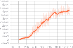
(1.) alien

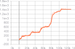
(2.) amidar

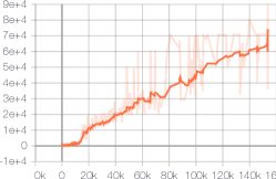
(3.) assault

(4.) asterix

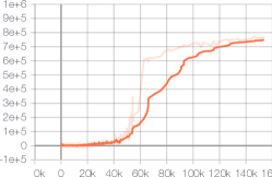
(5.) asteroids

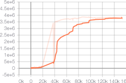
(6.) atlantis

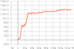
(7.) bank_heist

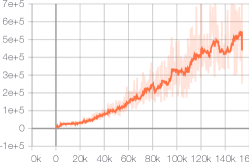
(8.) battle_zone

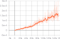
(9.) beam_rider

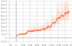
(10.) berzerk

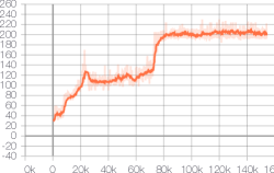
(11.) bowling

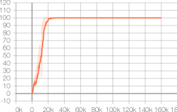
(12.) boxing

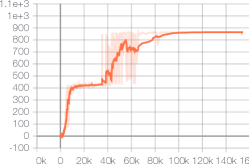
(13.) breakout

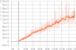
(14.) centipede

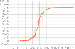
(15.) chopper_command

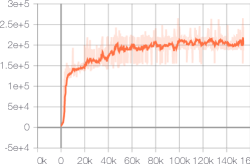
(16.) crazy_climber

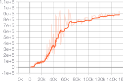
(17.) defender

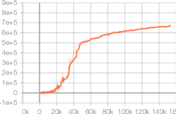
(18.) demon_attack

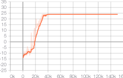
(19.) double_dunk

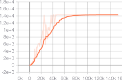
(20.) enduro

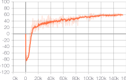
(21.) fishing_derby

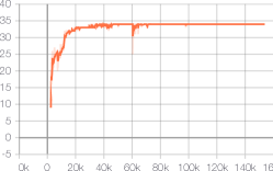
(22.) freeway

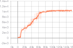
(23.) frostbite

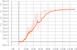
(24.) gopher

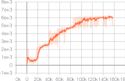
(25.) gravitar

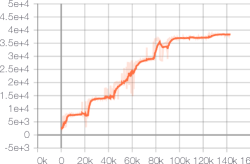
(26.) hero

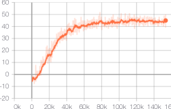
(27.) ice_hockey

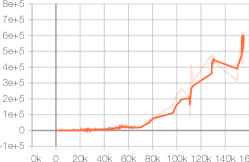
(28.) jamesbond

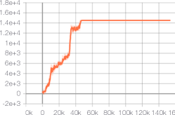
(29.) kangaroo

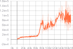
(30.) krull

(31.) kung_fu_master

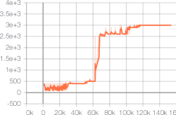
(32.) montezuma_revenge

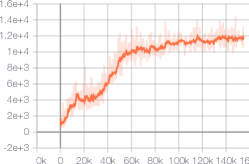
(33.) ms_pacman

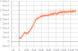
(34.) name_this_game

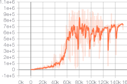
(35.) phoenix

(36.) pitfall

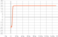
(37.) pong

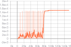
(38.) private_eye

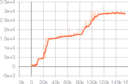
(39.) qbert

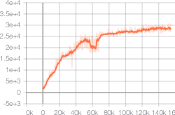
(40.) riverraid

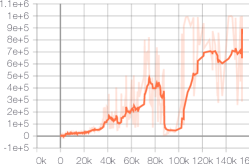
(41.) road_runner

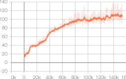
(42.) robotank

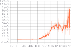
(43.) seaquest

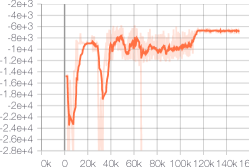
(44.) skiing

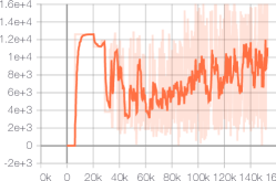
(45.) solaris

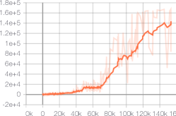
(46.) space_invaders

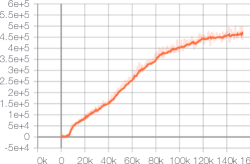
(47.) star_gunner

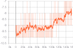
(48.) surround

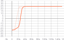
(49.) tennis

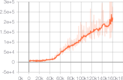
(50.) time_pilot

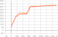
(51.) tutankham

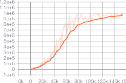
(52.) up_n_down

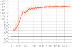
(53.) venture

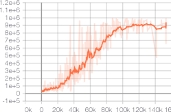
(54.) video_pinball

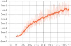
(55.) wizard_of_wor

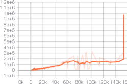
(56.) yars_revenge

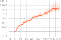
(57.) zaxxon

J.8.2 Atari Games Learning Curves of GDI-H³

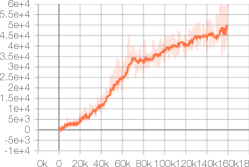
(1.) alien

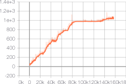
(2.) amidar

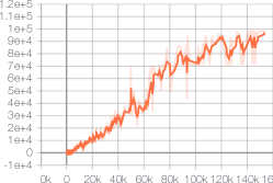
(3.) assault

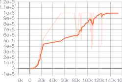
(4.) asterix

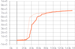
(5.) asteroids

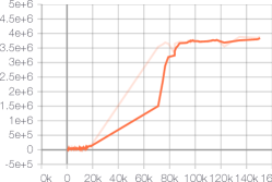
(6.) atlantis

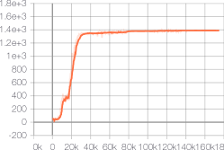
(7.) bank_heist

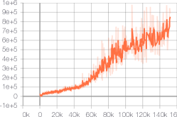
(8.) battle_zone

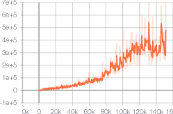
(9.) beam_rider

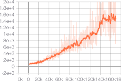
(10.) berzerk

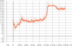
(11.) bowling

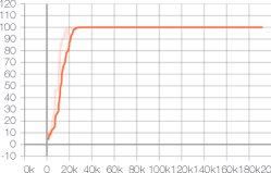
(12.) boxing

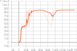
(13.) breakout

(14.) centipede

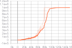
(15.) chopper_command

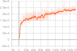
(16.) crazy_climber

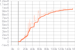
(17.) defender

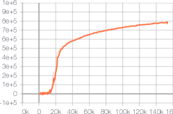
(18.) demon_attack

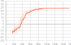
(19.) double_dunk

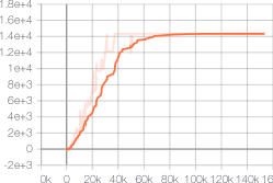
(20.) enduro

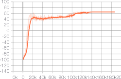
(21.) fishing_derby

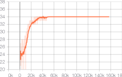
(22.) freeway

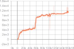
(23.) frostbite

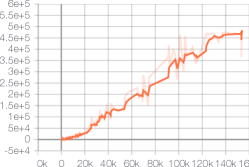
(24.) gopher

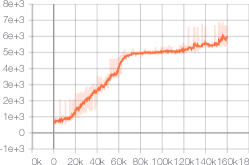
(25.) gravitar

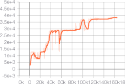
(26.) hero

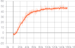
(27.) ice_hockey

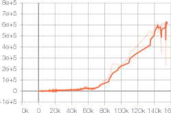
(28.) jamesbond

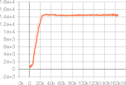
(29.) kangaroo

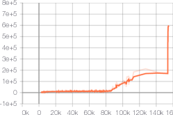
(30.) krull

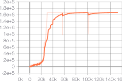
(31.) kung_fu_master

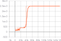
(32.) montezuma_revenge

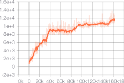
(33.) ms_pacman

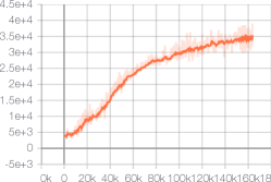
(34.) name_this_game

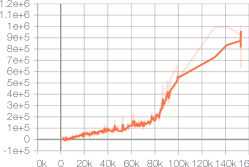
(35.) phoenix

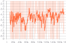
(36.) pitfall

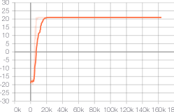
(37.) pong

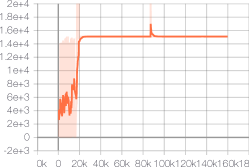
(38.) private_eye

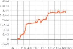
(39.) qbert

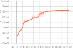
(40.) riverraid

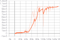
(41.) road_runner

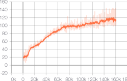
(42.) robotank

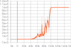
(43.) seaquest

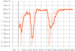
(44.) skiing

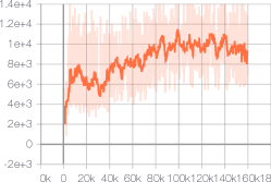
(45.) solaris

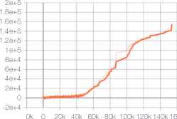
(46.) space_invaders

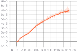
(47.) star_gunner

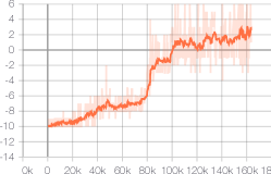
(48.) surround

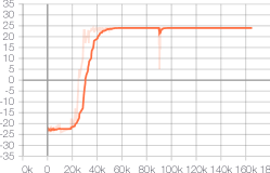
(49.) tennis

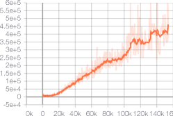
(50.) time_pilot

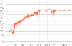
(51.) tutankham

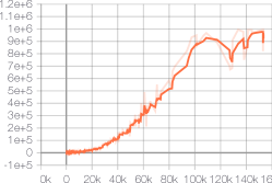
(52.) up_n_down

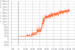
(53.) venture

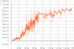
(54.) video_pinball

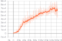
(55.) wizard_of_wor

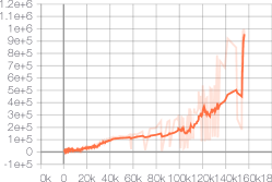
(56.) yars_revenge

(57.) zaxxon

Appendix K Ablation Study

In this section, we firstly demonstrate the settings of our ablation studies. Then, we illustrate the performance graphs among all ablation cases in three representative Atari games. Lastly, we offer the t-SNE of three Atari games to further prove expansion of policy space in GDI brings more diverse data and more chance to obtain elite data.

K.1 Ablation Study Details

The details of ablation changes are listed in Tab. 20. All the ablation studies are carried out using the evaluation system and 200M training frames. The operator $\mathcal{T}$ is achieved with Vtrace, Retrace and policy gradient. Except for the differences listed in the table, other settings and the shared hyperparameters remain the same in all ablation cases. The hyperparameters can see App. I.2.

Table 20: Settings of ablation study.

Name	Category	$\Lambda$	$P_{\Lambda}^{(0)}$	$\mathcal{E}$
GDI-I3	GDI-I3	$\Lambda=\{\lambda|\lambda=(\epsilon,\tau_{1},\tau_{2})\}$	Uniform	MAB
GDI-H3	GDI-H3	$\Lambda=\{\lambda|\lambda=(\epsilon,\tau_{1},\tau_{2})\}$	Uniform	MAB
Fix Selection	GDI-I0 w/o $\mathcal{E}$	$\Lambda=\{\lambda|\lambda=(\epsilon,\tau_{1},\tau_{2})\}$	Delta	Identical Mapping
Random Selection	GDI-I3 w/o $\mathcal{E}$	$\Lambda=\{\lambda|\lambda=(\epsilon,\tau_{1},\tau_{2})\}$	Uniform	Identical Mapping
Boltzmann Selection	GDI-I1	$\Lambda=\{\lambda|\lambda=(\tau)\}$	Uniform	MAB
$\epsilon$-greedy Selection	GDI-I1	$\Lambda=\{\lambda|\lambda=(\epsilon)\}$	Uniform	MAB

K.2 Ablation Results

In this part, we show three representative experiments of different Atari games among all the ablation cases in Figs. 18.

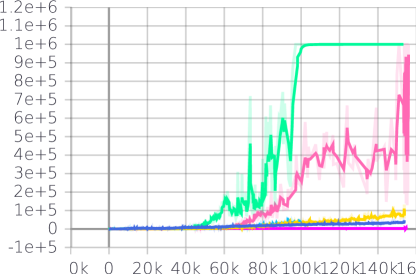
(1.) Seaquest

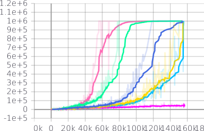
(2.) ChopperCommand

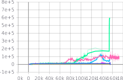
(3.) Krull

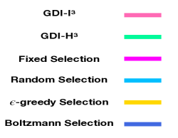
Figure 18: Evaluation curves of ablation study. For ease of comparison, all curves are smoothed with rate 0.9.

K.3 t-SNE

In all the t-SNE, we mark the state generated by GDI-I³ as A_i and mark the state generated by GDI-I¹ as B_i, where i = 1, 2, 3 represents three stages of the training process. WLOG, we choose the Boltzmann Selection as the representative of GDI-I¹ algorithms.

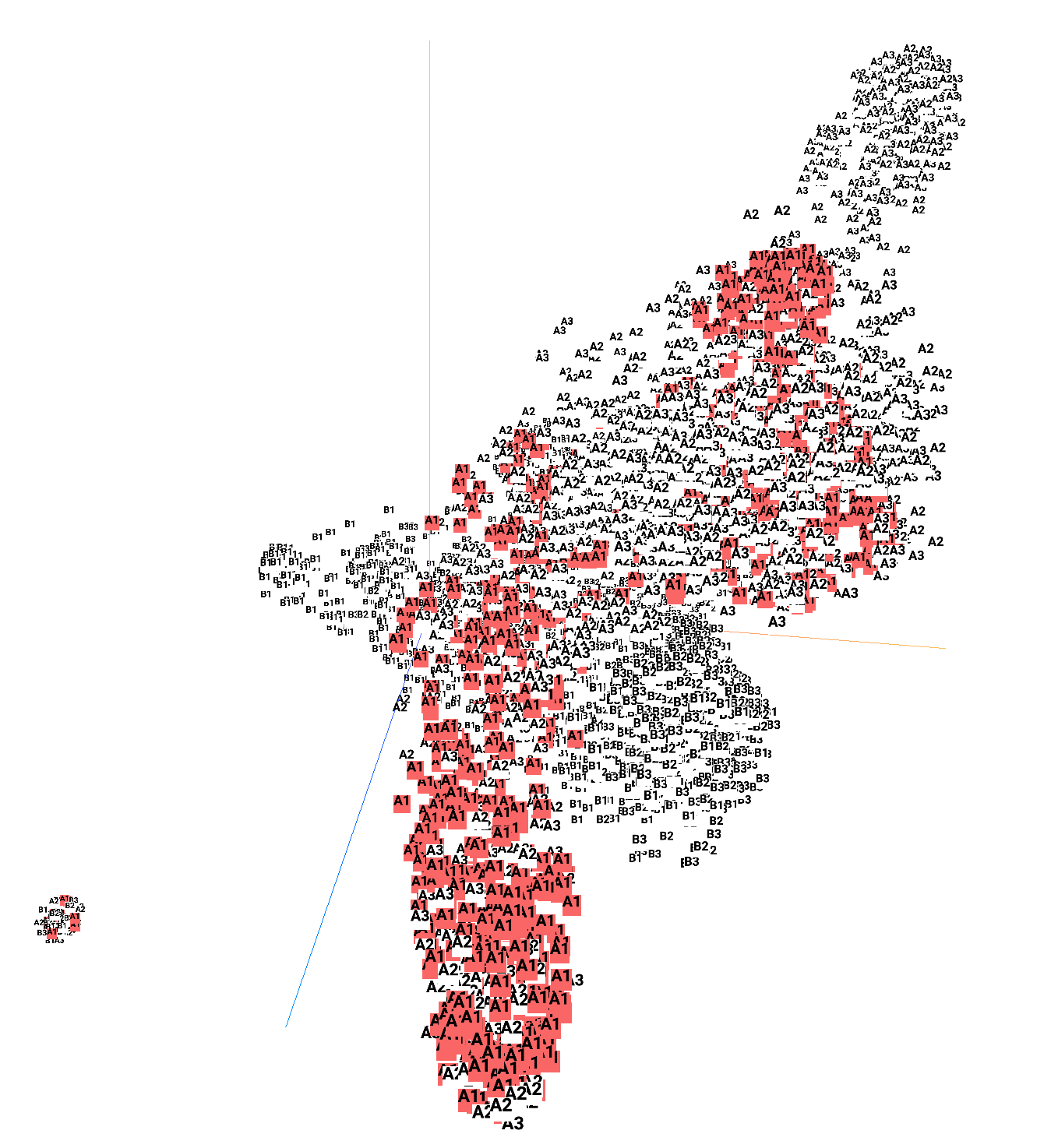
(1.) Early stage of GDI-I³

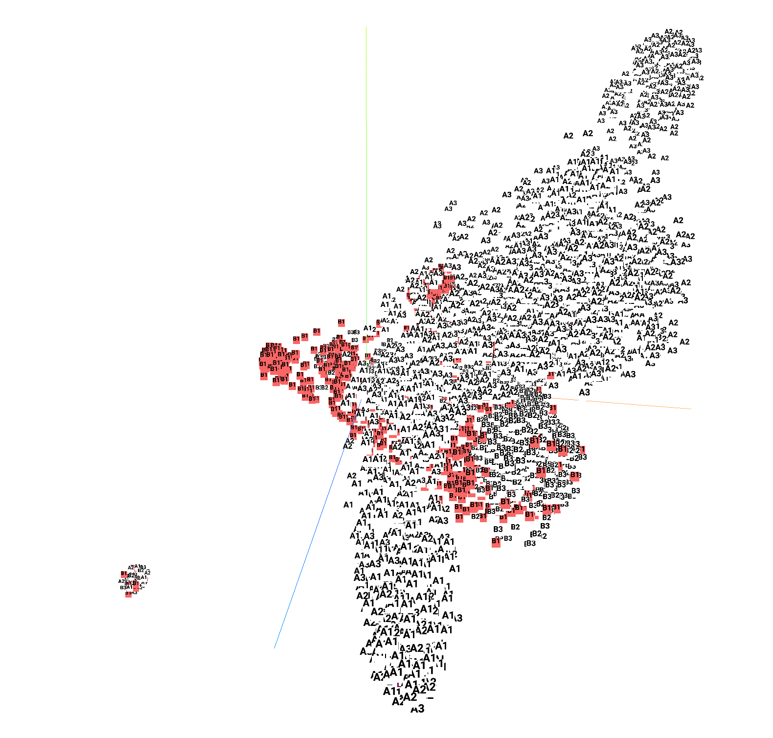
(2.) Early stage of GDI-I¹

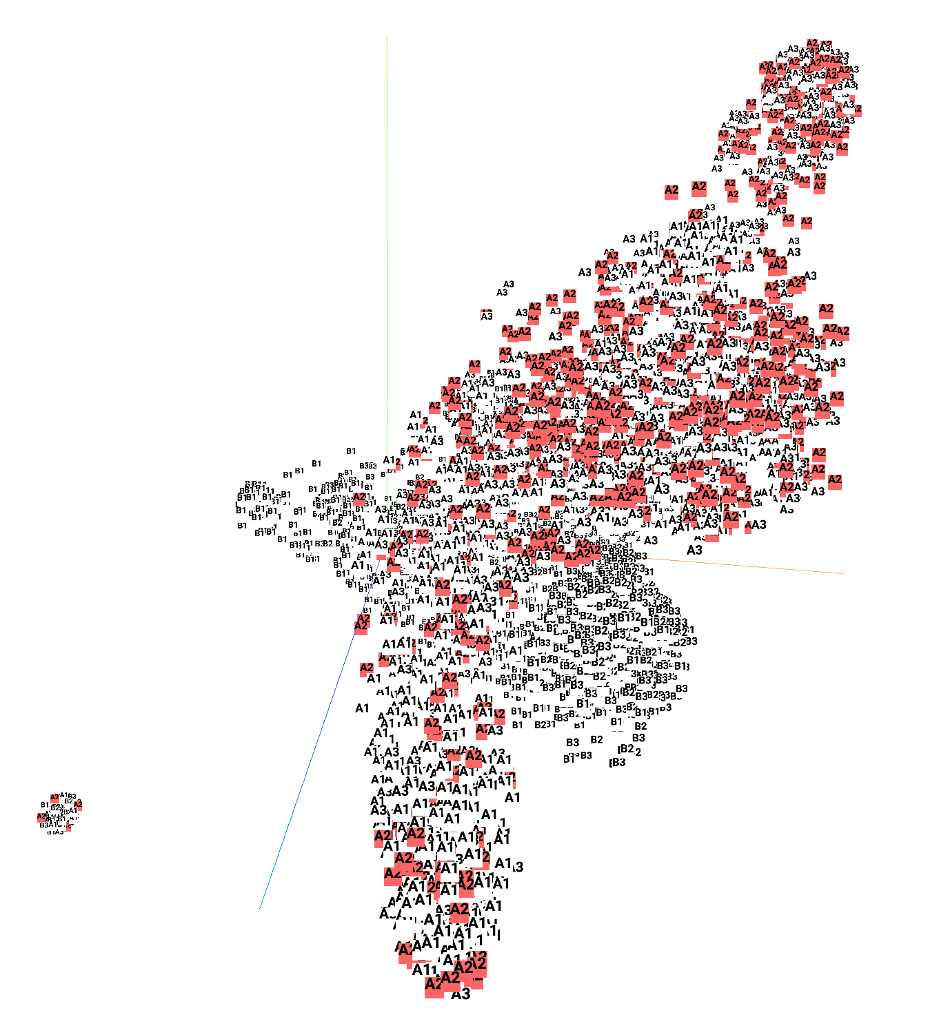
(3.) Middle stage of GDI-I³

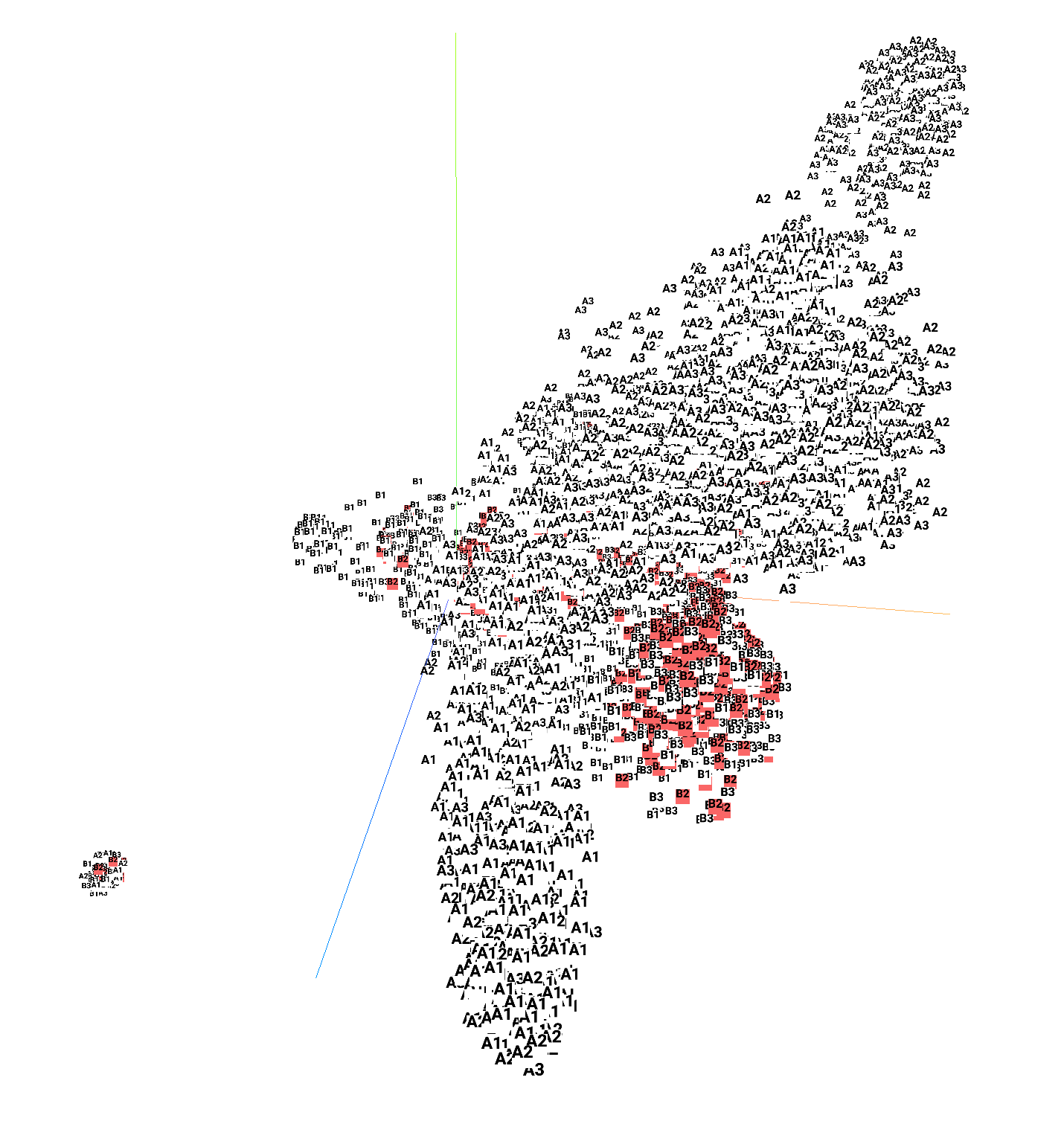
(4.) Middle stage of GDI-I¹

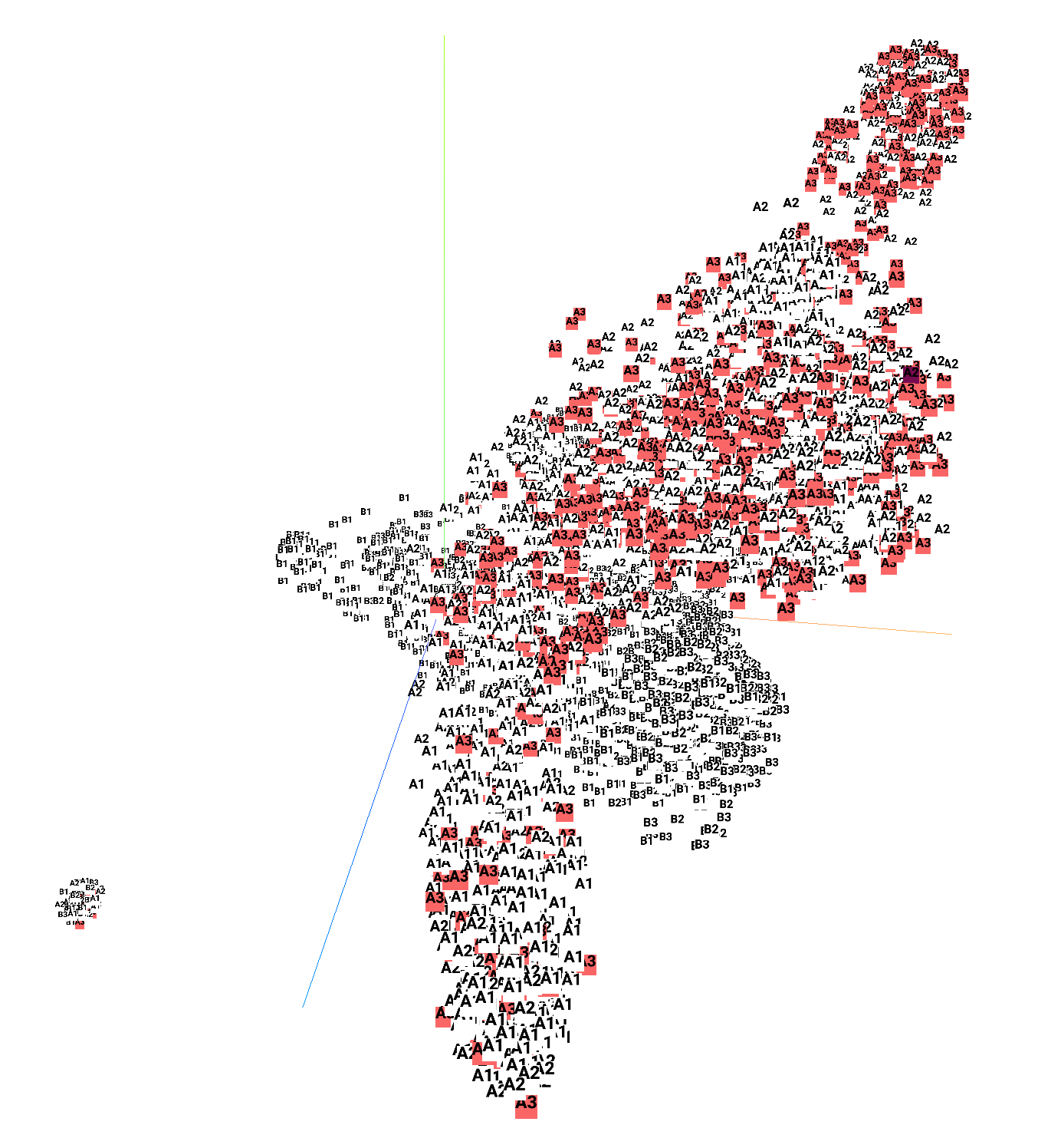
(5.) Later stage of GDI-I³

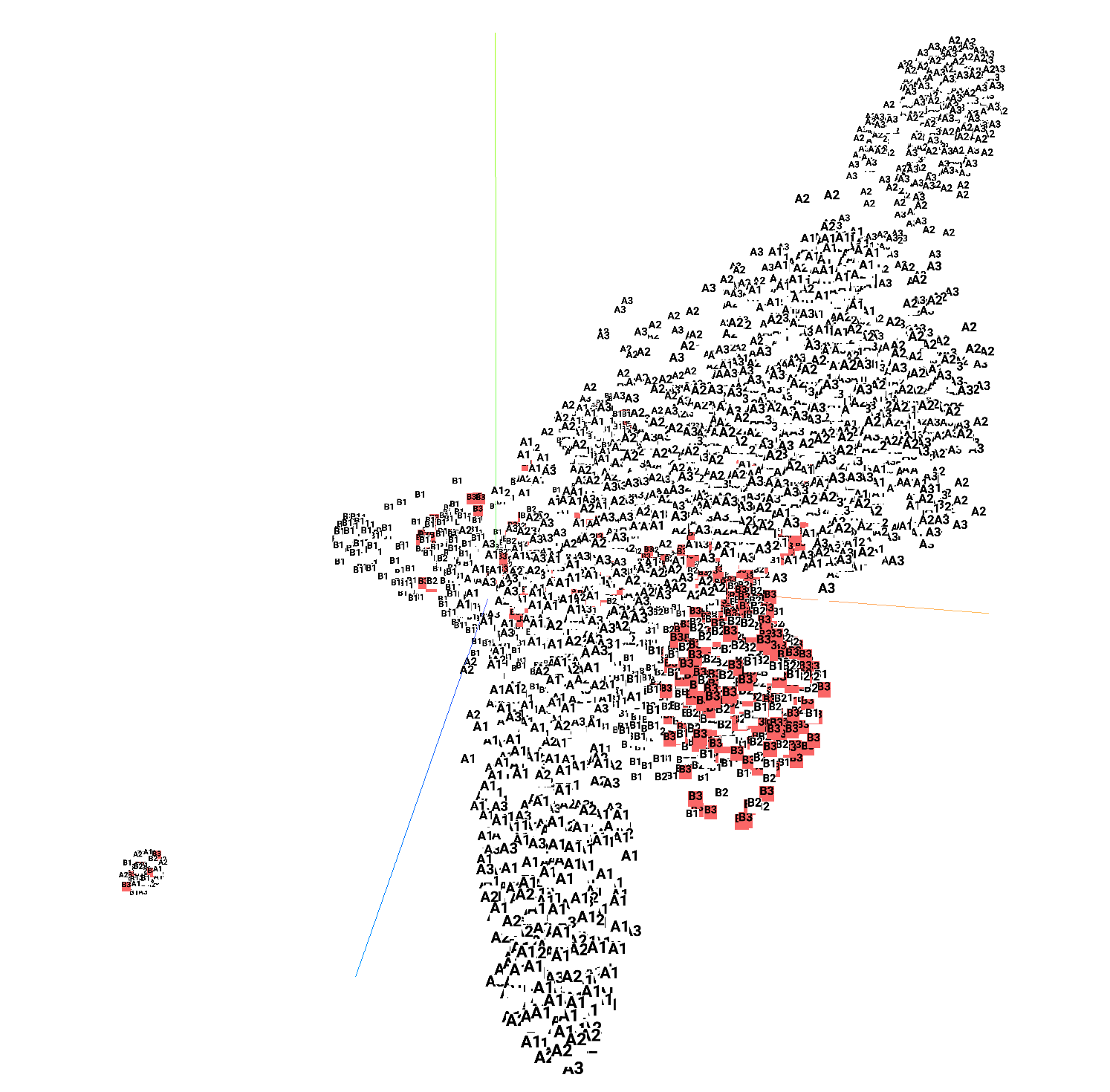
(6.) Later stage of GDI-I¹

Figure 19: t-SNE of Seaquest. t-SNE is drawn from 6k states. We sample 1k states from each stage of GDI-I³ and GDI-I¹. We highlight 1k states of each stage of GDI-I³ and GDI-I¹.

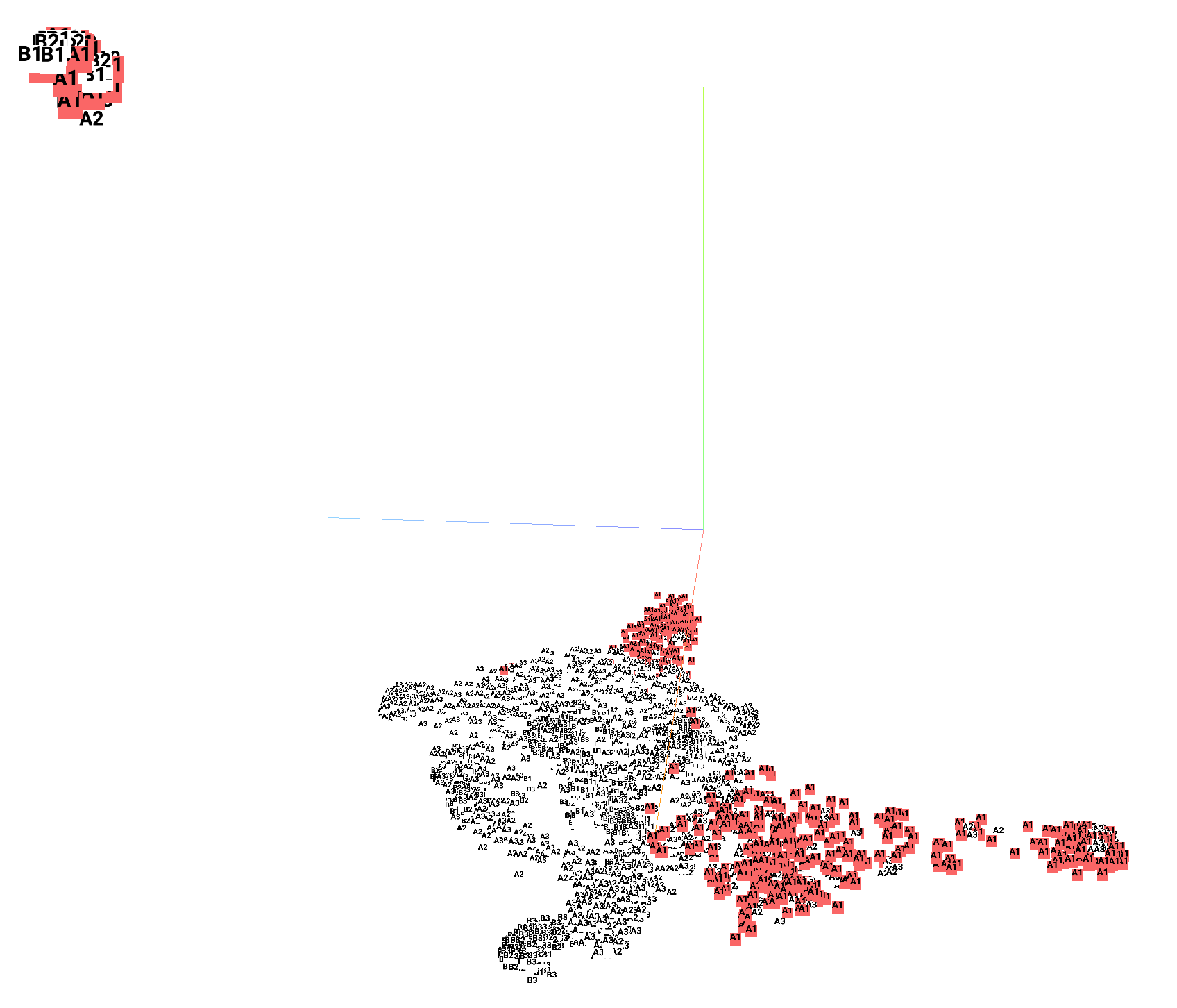
(1.) Early stage of GDI-I³

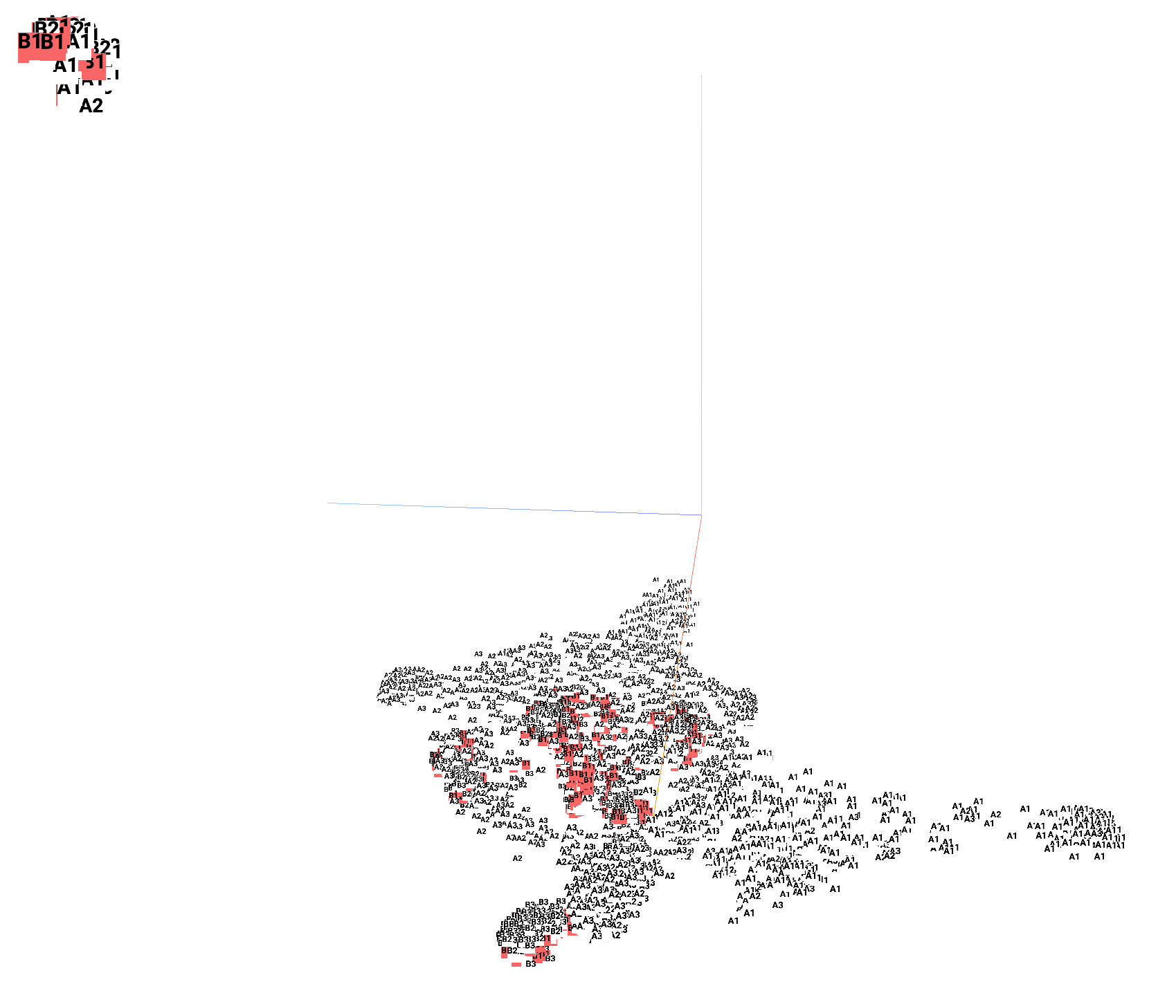
(2.) Early stage of GDI-I¹

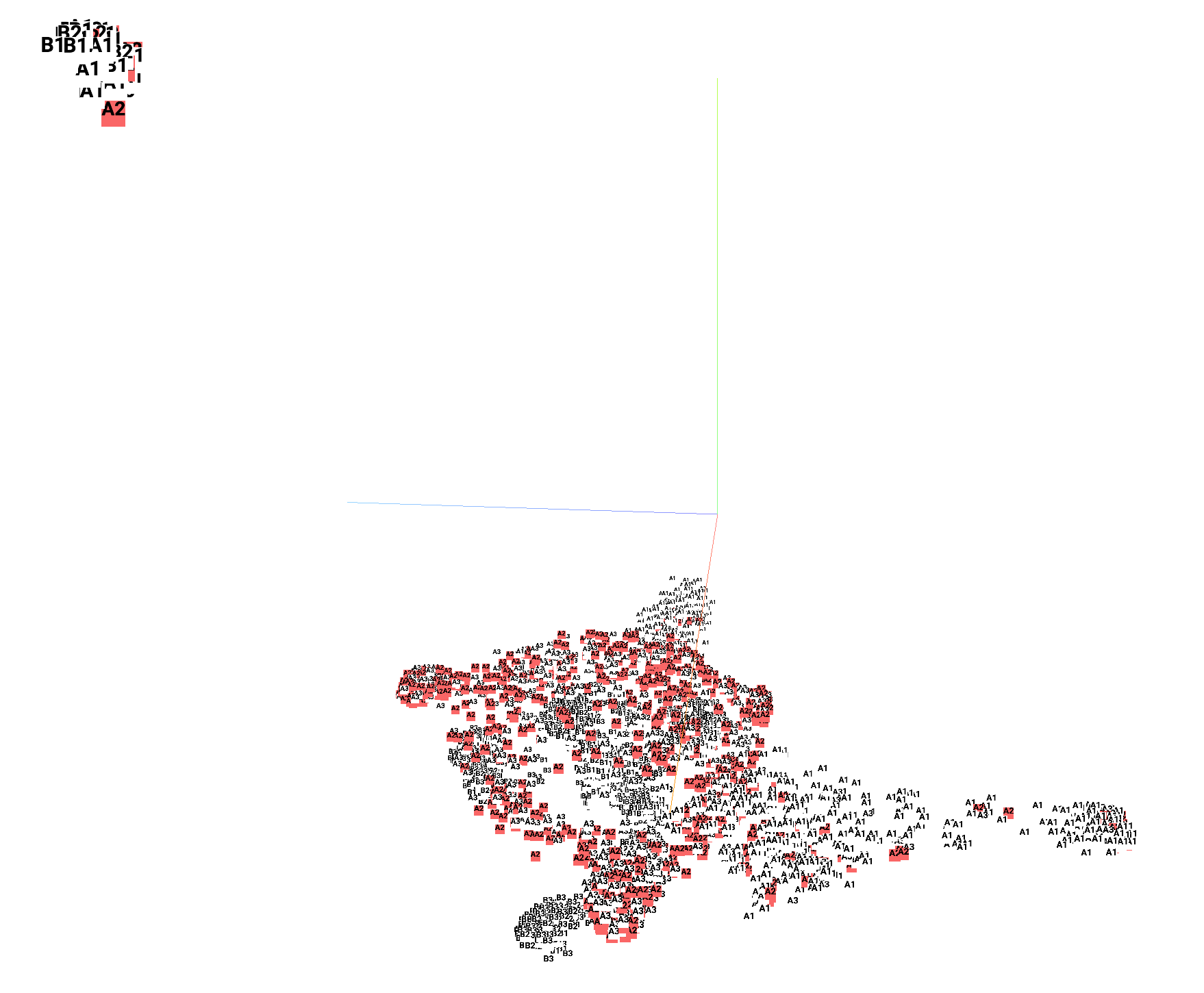
(3.) Middle stage of GDI-I³

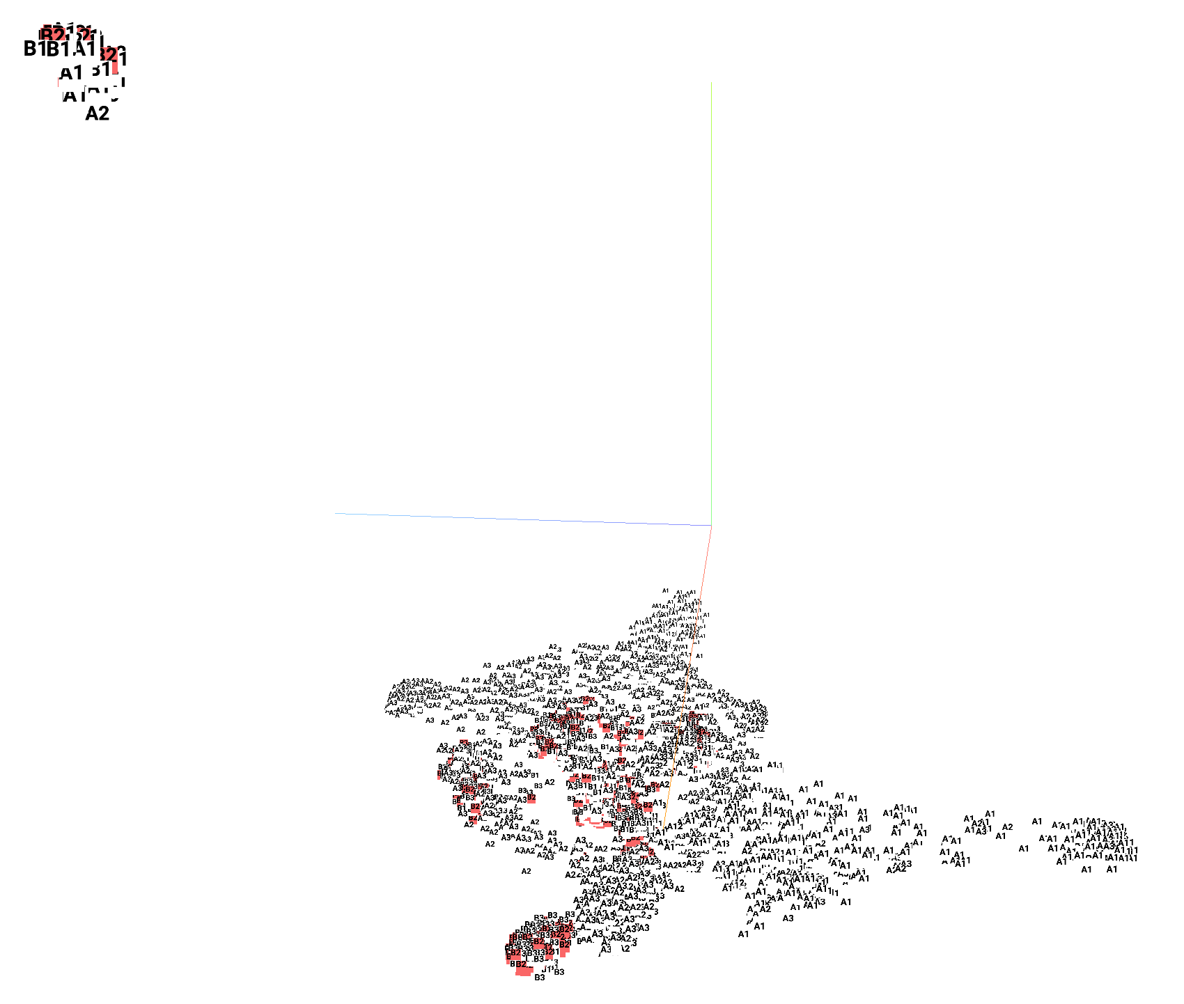
(4.) Middle stage of GDI-I¹

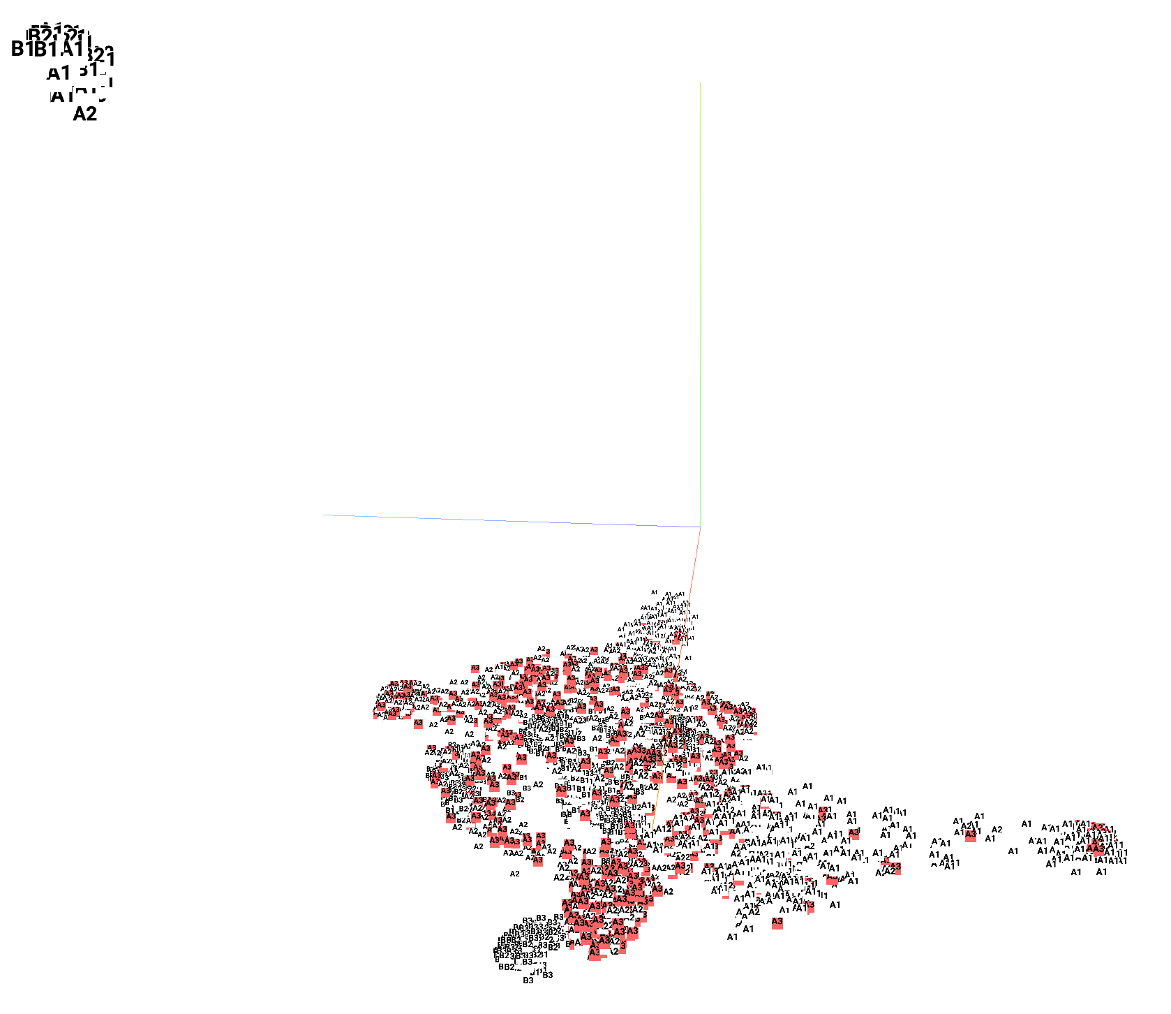
(5.) Later stage of GDI-I³

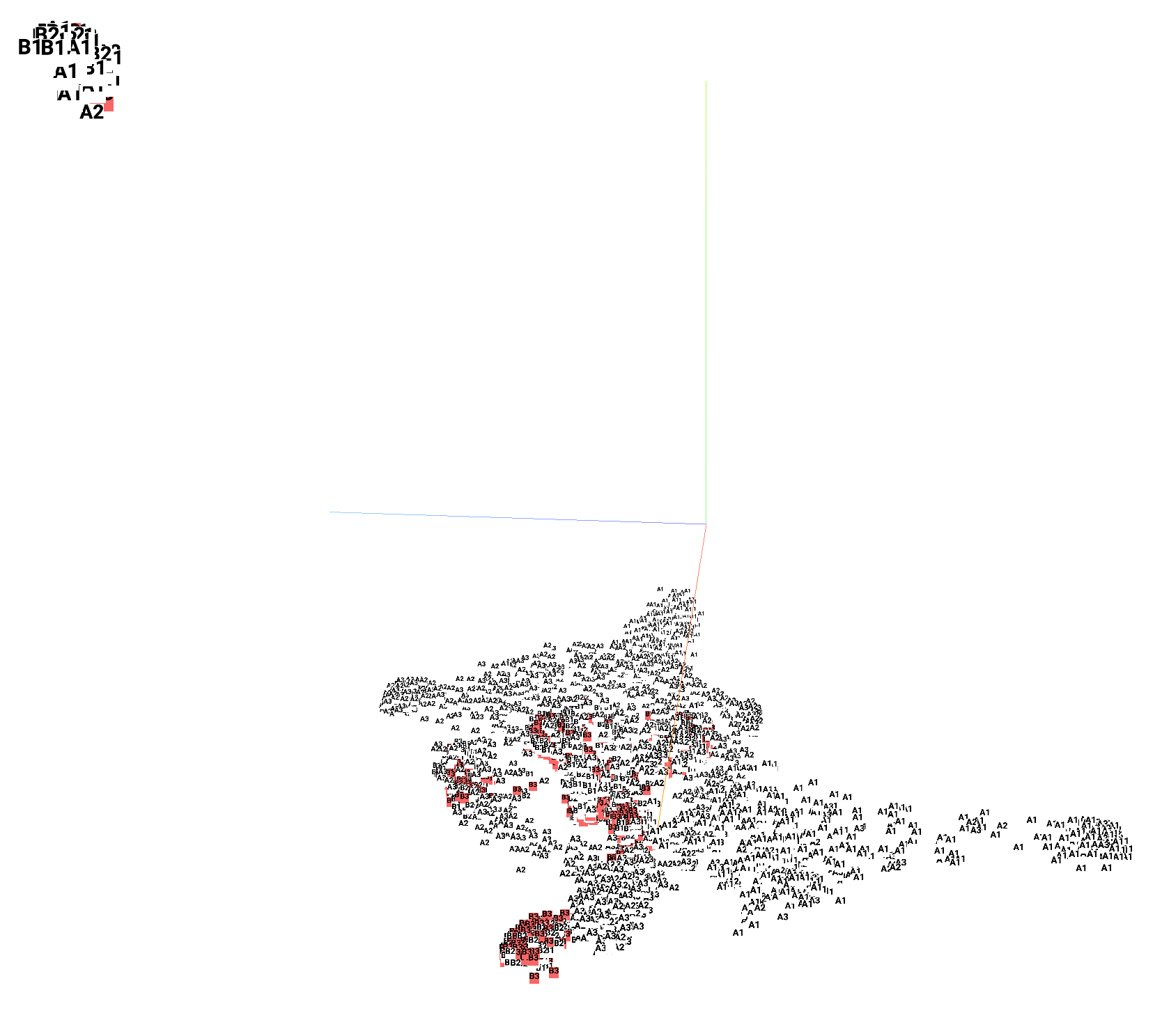
(6.) Later stage of GDI-I¹

Figure 20: t-SNE of ChopperCommand. t-SNE is drawn from 6k states. We sample 1k states from each stage of GDI-I³ and GDI-I¹. We highlight 1k states of each stage of GDI-I³ and GDI-I¹.

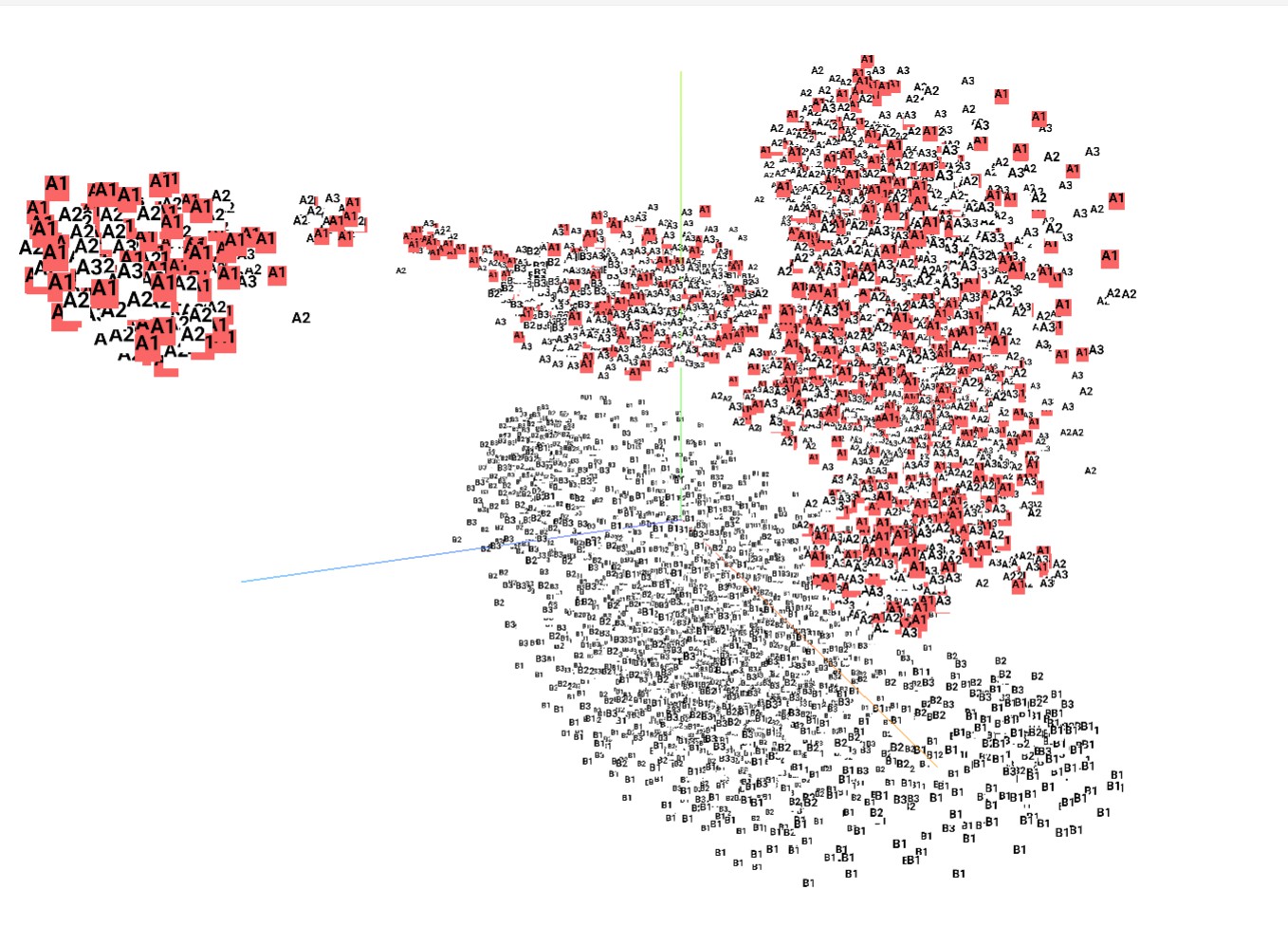
(1.) Early stage of GDI-H³

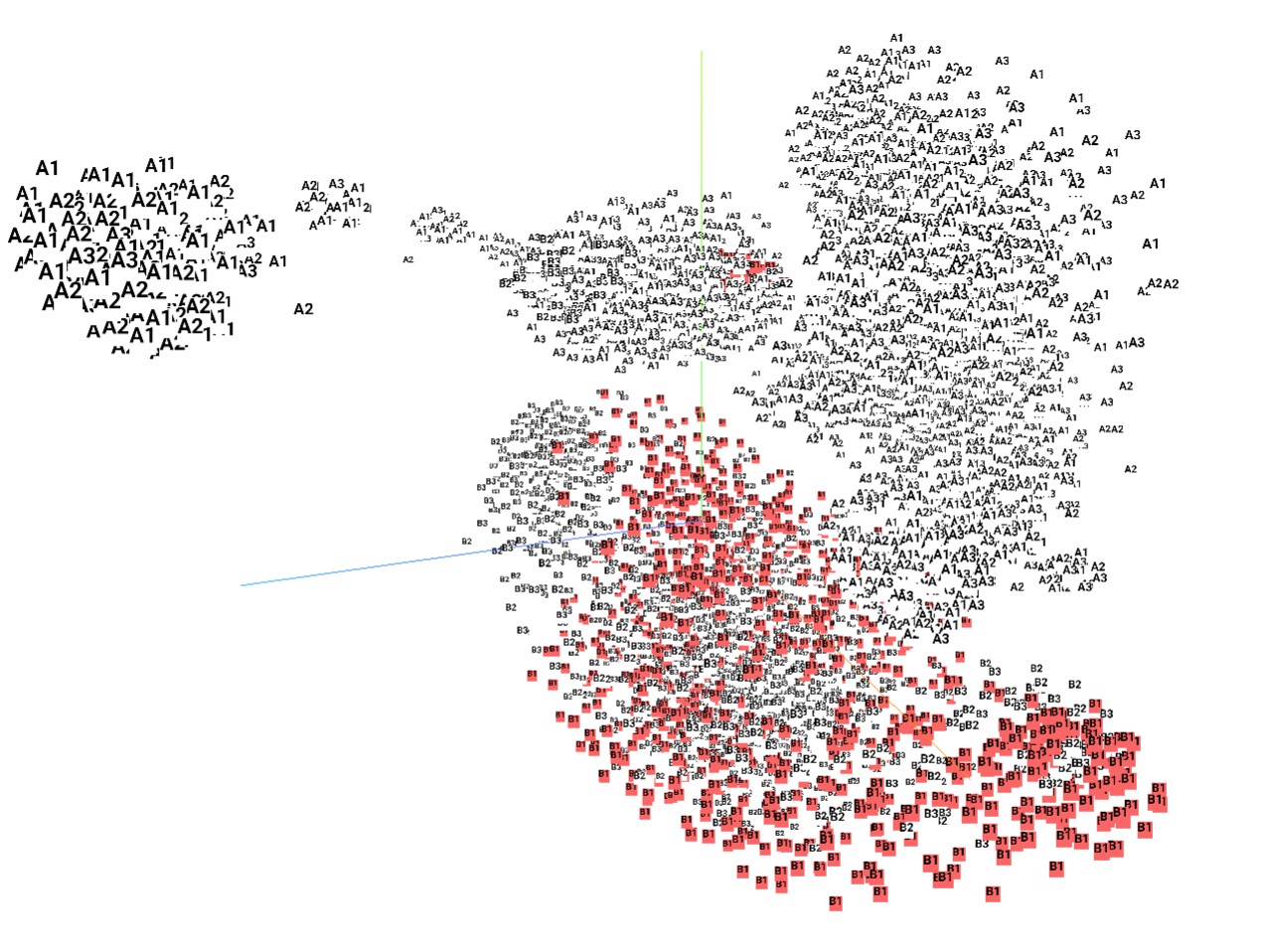
(2.) Early stage of GDI-I¹

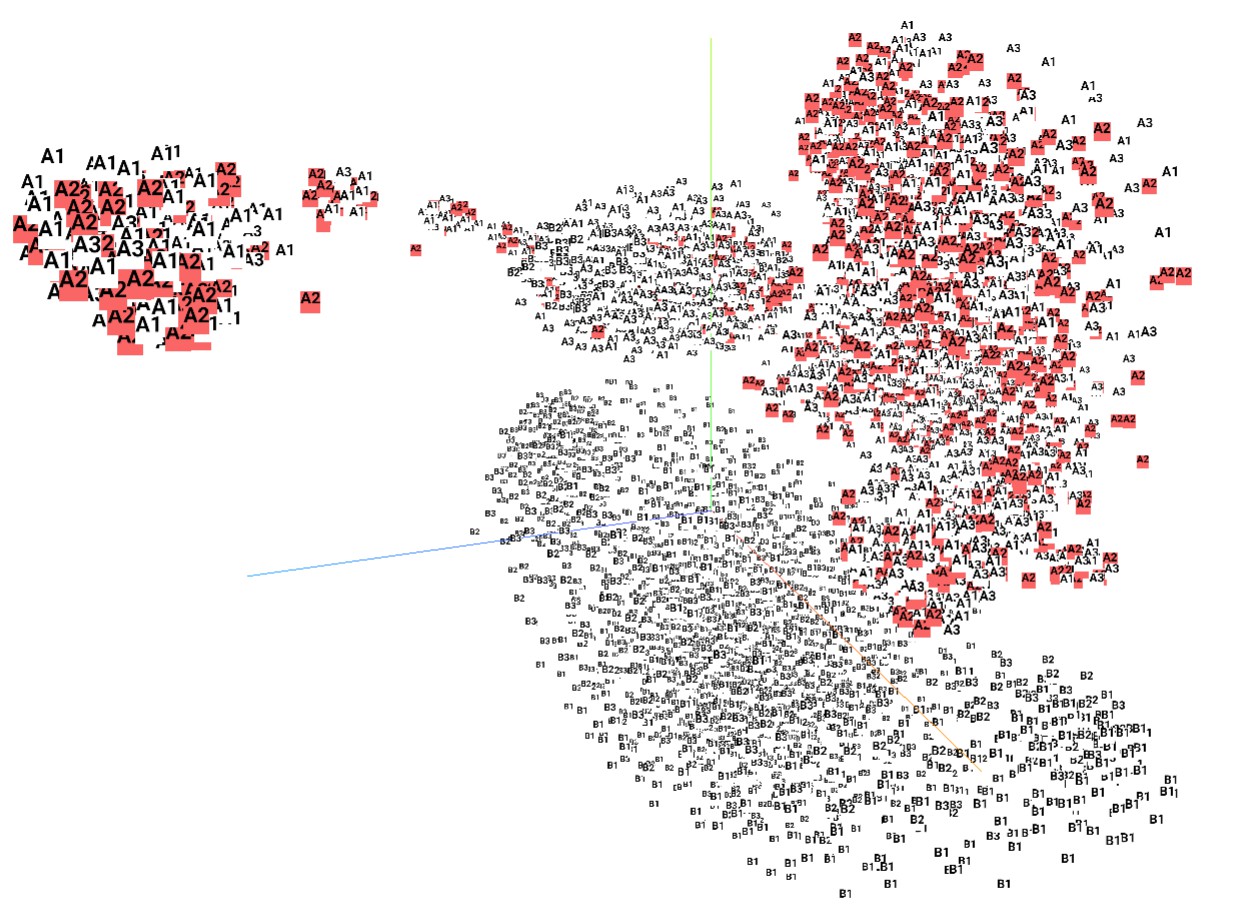
(3.) Middle stage of GDI-H³

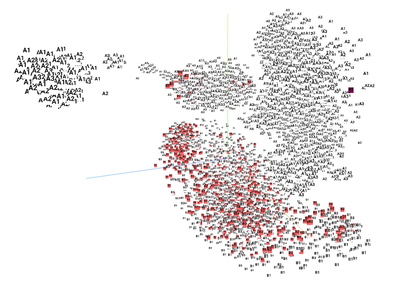
(4.) Middle stage of GDI-I¹

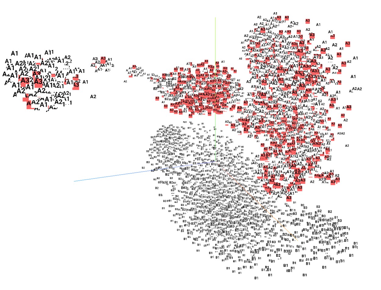
(5.) Later stage of GDI-H³

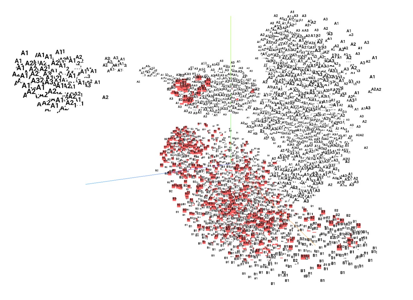
(6.) Later stage of GDI-I¹

Figure 21: t-SNE of Krull. t-SNE is drawn from 6k states. We sample 1k states from each stage of GDI-H³ and GDI-I¹. We highlight 1k states of each stage of GDI-H³ and GDI-I¹.

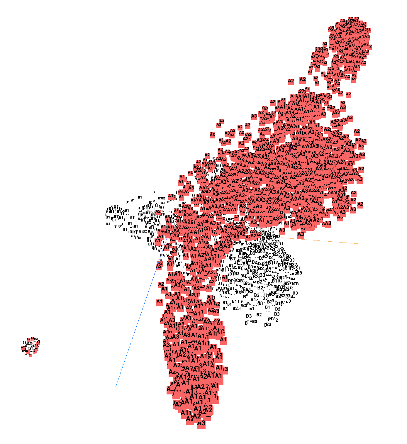
(1.) GDI-I³ on Seaquest

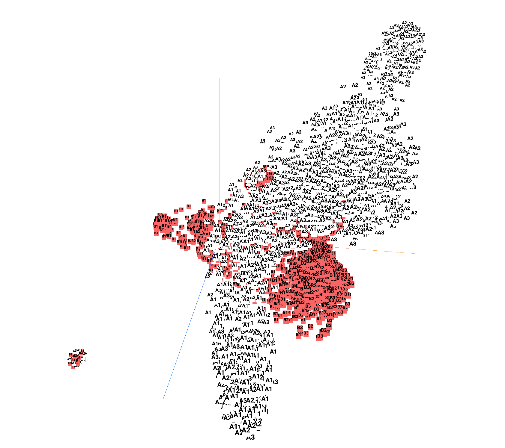
(2.) GDI-I¹ on Seaquest

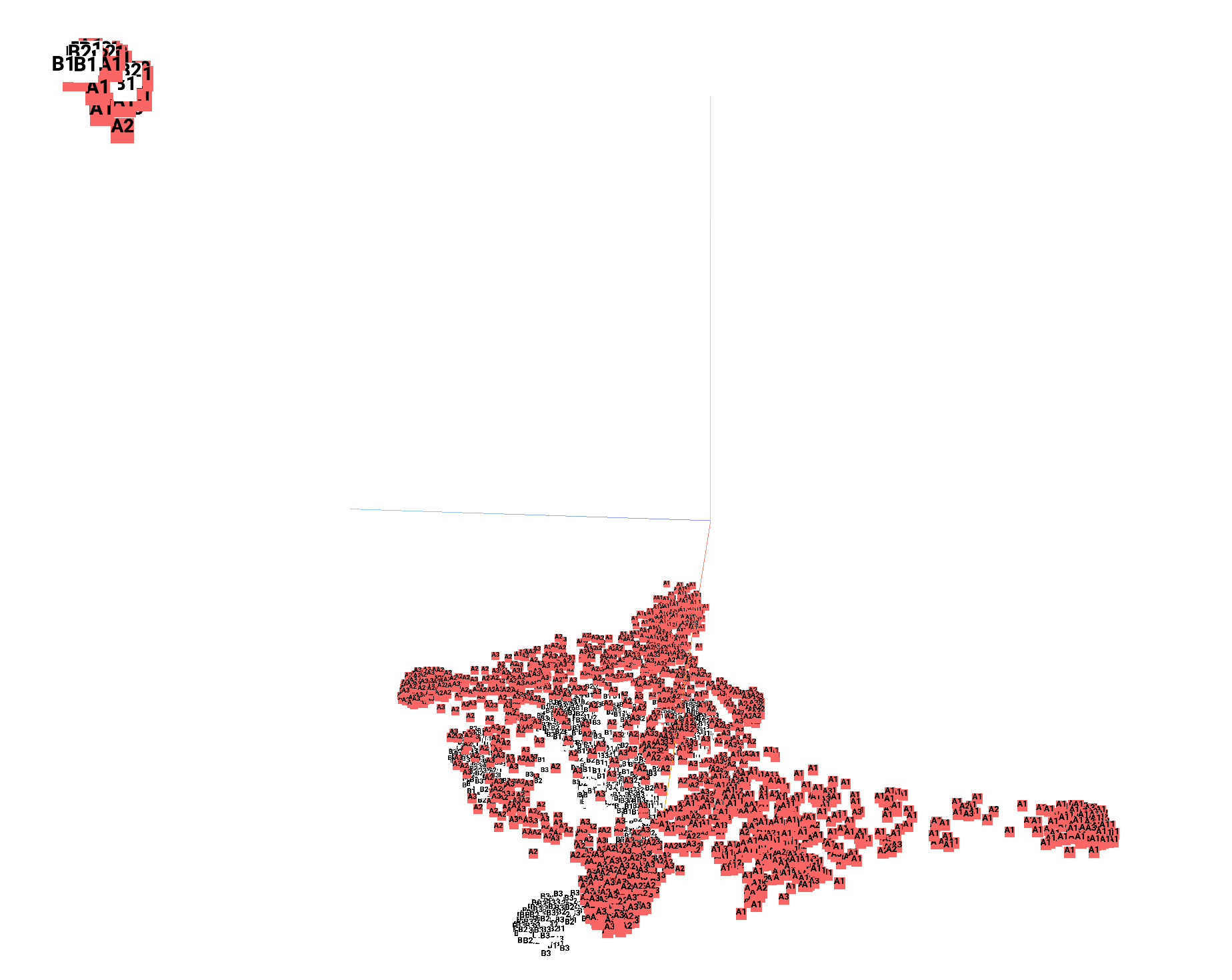
(3.) GDI-I³ on ChopperCommand

(4.) GDI-I¹ on ChopperCommand

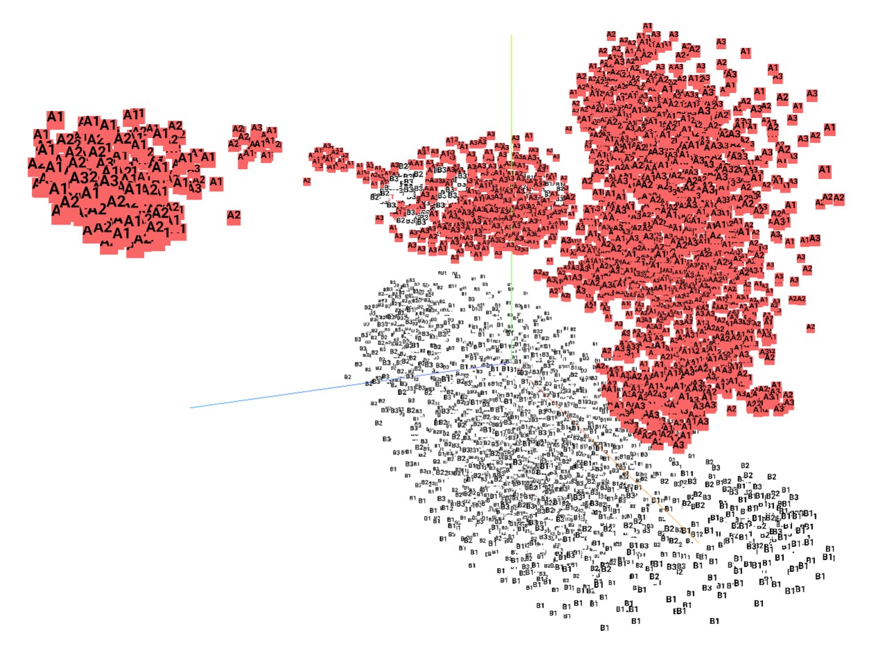
(5.) GDI-H³ on Krull

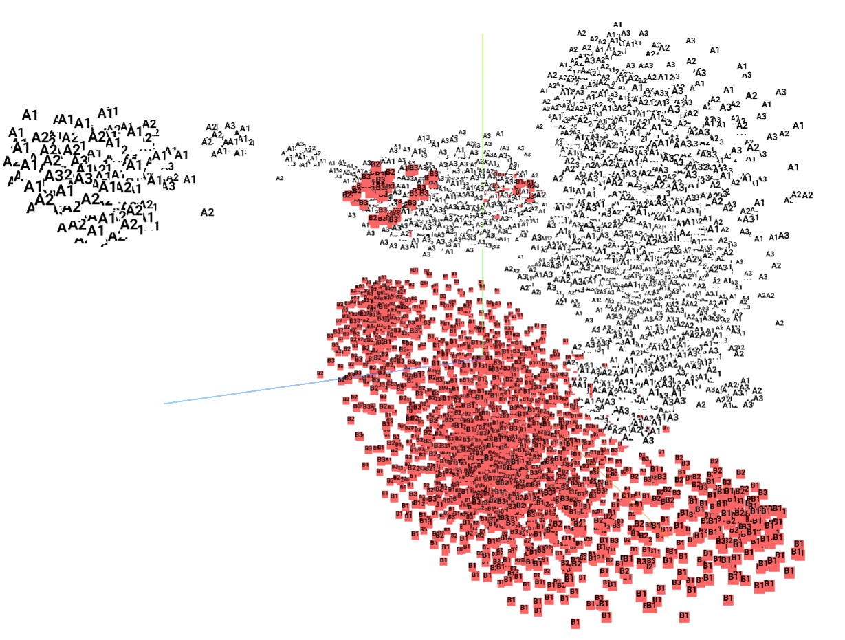
(6.) GDI-I¹ on Krull

Figure 22: Overview of t-SNE in Atari games. Each t-SNE figure is drawn from 6k states. We highlight 3k states of GDI-I³, GDI-H³ and GDI-I¹, respectively.

K.4 Table of Score

Games	Fix Selection	HNS(%)	Boltzmann Selection	HNS(%)	GDI-I3	HNS(%)	GDI-H3	HNS(%)
Category	GDI-I0 w/o $\mathcal{E}$		GDI-I1		GDI-I3		GDI-H3
Scale	200M		200M		200M		200M
alien	13720	195.54	10641	150.92	43384	625.45	48735	703.00
amidar	560	32.34	653.9	37.82	1442	83.81	1065	61.81
assault	16228	3080.37	36251	6933.91	63876	12250.50	97155	18655.23
asterix	213580	2572.80	851210	10261.30	759910	9160.41	999999	12055.38
asteroids	18621	38.36	759170	1625.15	751970	1609.72	760005	1626.94
atlantis	3211600	19772.10	3670700	22609.89	3803000	23427.66	3837300	23639.67
bank heist	895.3	119.24	1381	184.98	1401	187.68	1380	184.84
battle zone	70137	189.17	130410	352.28	478830	1295.20	824360	2230.29
beam rider	34920	208.64	104030	625.90	162100	976.51	422390	2548.07
berzerk	1648	60.81	1222	43.81	7607	298.53	14649	579.46
bowling	162.4	101.24	176.4	111.41	202	129.94	205.2	132.34
boxing	98.3	818.33	99.9	831.67	100	832.50	100	832.50
breakout	624.3	2161.81	696	2410.76	864	2994.10	864	2994.10
centipede	102600	1012.57	38938	371.21	155830	1548.84	195630	1949.80
chopper command	66690	1001.69	999999	15192.62	999999	15192.62	999999	15192.62
crazy climber	161250	600.70	157250	584.73	201000	759.39	241170	919.76
defender	421600	2647.75	837750	5279.21	893110	5629.27	970540	6118.89
demon attack	291590	16022.76	549450	30199.46	675530	37131.12	787985	43313.70
double dunk	20.25	1765.91	23	1890.91	24	1936.36	24	1936.36
enduro	10019	1164.32	14317	1663.80	14330	1665.31	14300	1661.82
fishing derby	53.24	273.99	48.8	265.60	59	285.71	65	296.22
freeway	3.46	11.69	33.7	113.85	34	114.86	34	114.86
frostbite	1583	35.55	8102	188.24	10485	244.05	11330	263.84
gopher	188680	8743.90	454150	21063.27	488830	22672.63	473560	21964.01
gravitar	4311	130.19	6150	188.05	5905	180.34	5915	180.66
hero	24236	77.88	17655	55.80	38330	125.18	38225	124.83
ice hockey	1.56	105.45	-8.1	25.62	44.94	463.97	47.11	481.90
jamesbond	12468	4543.10	567020	207082.18	594500	217118.70	620780	226716.95
kangaroo	5399	179.25	14286	477.17	14500	484.34	14636	488.90
krull	12104.7	984.23	11104	890.49	97575	8990.82	594540	55544.92
kung fu master	124630.1	553.31	1270800	5652.43	140440	623.64	1666665	7413.57
montezuma revenge	2488.4	52.35	2528	53.18	3000	63.11	2500	52.60
ms pacman	7579	109.44	4296	60.03	11536	169.00	11573	169.55
name this game	32098	517.76	30037	481.95	34434	558.34	36296	590.68
phoenix	498590	7681.23	597580	9208.60	894460	13789.30	959580	14794.07
pitfall	-17.8	3.16	-21.8	3.10	0	3.43	-4.3	3.36
pong	20.39	116.40	21	118.13	21	118.13	21	118.13
private eye	134.1	0.16	15095	21.67	15100	21.68	15100	21.68
qbert	21043	157.09	19091	142.40	27800	207.93	28657	214.38
riverraid	11182	62.38	17081	99.77	28075	169.44	28349	171.17
road runner	251360	3208.64	57102	728.80	878600	11215.78	999999	12765.53
robotank	10.44	84.95	69.7	695.88	108	1092.78	113.4	1146.39
seaquest	2728	6.33	11862	28.09	943910	2247.98	1000000	2381.57
skiing	-12730	34.23	-9327	60.90	-6774	80.90	-6025	86.77
solaris	2319	9.76	3653	21.79	11074	88.70	9105	70.95
space invaders	3031	189.58	105810	6948.25	140460	9226.80	154380	10142.17
star gunner	337150	3510.18	358650	3734.47	465750	4851.72	677590	7061.61
surround	-9.9998	0.00	-9.8	1.21	-8	13.33	2.606	76.40
tennis	-21.05	17.74	23.7	306.45	24	308.39	24	308.39
time pilot	84341	4862.62	150930	8871.35	216770	12834.99	450810	26924.45
tutankham	381	236.62	380.3	236.17	424	264.08	418.2	260.44
up n down	416020	3723.06	907170	8124.13	986440	8834.45	966590	8656.58
venture	0	0.00	1969	165.81	2035	171.37	2000	168.42
video pinball	297920	1686.22	673840	3813.92	925830	5240.18	978190	5536.54
wizard of wor	26008	606.83	21325	495.15	64293	1519.90	63735	1506.59
yars revenge	76903.5	143.37	84684	158.48	972000	1881.96	968090	1874.36
zaxxon	46070.8	503.66	62133	679.38	109140	1193.63	216020	2362.89
MEAN HNS(%)		1783.24		6712.31		7810.6		9620.98
MEDIAN HNS(%)		195.54		477.17		832.5		1146.39

Table 21: Score table of the ablation study on HNS.

Appendix L Videos

In the future, we will put all the videos of the performance of our algorithm on sites, which will contain the following:

• Our performance on all Atari games: We provide an example video for each game in the Atari games sweep, wherein our algorithm surpass all the existing SOTA algorithms and achieves SOTA.

• Adaptive Entropy Control: We show example videos for algorithms in the game James Bond, wherein the agents automatically learns how to trade off the exploitation policy and exploration.

• Human World Records Breakthroughs: We also provide an example video for 22 Atari games, wherein our algorithms achieved 22 human world records breakthroughs.

References

- Agarwal et al. (2019) Agarwal Alekh, Kakade Sham M, Lee Jason D, Mahajan Gaurav. On the theory of policy gradient methods: Optimality, approximation, and distribution shift // arXiv preprint arXiv:1908.00261. 2019.
- Angluin (1988) Angluin Dana. Queries and concept learning // Machine learning. 1988. 2, 4. 319–342.
- Badia et al. (2020a) Badia Adrià Puigdomènech, Piot Bilal, Kapturowski Steven, Sprechmann Pablo, Vitvitskyi Alex, Guo Daniel, Blundell Charles. Agent57: Outperforming the atari human benchmark // arXiv preprint arXiv:2003.13350. 2020a.
- Badia et al. (2020b) Badia Adrià Puigdomènech, Sprechmann Pablo, Vitvitskyi Alex, Guo Daniel, Piot Bilal, Kapturowski Steven, Tieleman Olivier, Arjovsky Martín, Pritzel Alexander, Bolt Andew, others . Never Give Up: Learning Directed Exploration Strategies // arXiv preprint arXiv:2002.06038. 2020b.
- Baum (1991) Baum Eric B. Neural net algorithms that learn in polynomial time from examples and queries // IEEE Transactions on Neural Networks. 1991. 2, 1. 5–19.
- Bellemare et al. (2013) Bellemare M. G., Naddaf Y., Veness J., Bowling M. The Arcade Learning Environment: An Evaluation Platform for General Agents // Journal of Artificial Intelligence Research. jun 2013. 47. 253–279.
- Berner et al. (2019) Berner Christopher, Brockman Greg, Chan Brooke, Cheung Vicki, Dębiak Przemysław, Dennison Christy, Farhi David, Fischer Quirin, Hashme Shariq, Hesse Chris, others . Dota 2 with large scale deep reinforcement learning // arXiv preprint arXiv:1912.06680. 2019.
- Cohn et al. (1996) Cohn David A, Ghahramani Zoubin, Jordan Michael I. Active learning with statistical models // Journal of artificial intelligence research. 1996. 4. 129–145.
- Dadashi et al. (2019) Dadashi Robert, Taiga Adrien Ali, Le Roux Nicolas, Schuurmans Dale, Bellemare Marc G. The value function polytope in reinforcement learning // International Conference on Machine Learning. 2019. 1486–1495.
- Ecoffet et al. (2019) Ecoffet Adrien, Huizinga Joost, Lehman Joel, Stanley Kenneth O, Clune Jeff. Go-explore: a new approach for hard-exploration problems // arXiv preprint arXiv:1901.10995. 2019.
- Espeholt et al. (2018) Espeholt Lasse, Soyer Hubert, Munos Remi, Simonyan Karen, Mnih Volodymir, Ward Tom, Doron Yotam, Firoiu Vlad, Harley Tim, Dunning Iain, others . Impala: Scalable distributed deep-rl with importance weighted actor-learner architectures // arXiv preprint arXiv:1802.01561. 2018.
- Eysenbach et al. (2018) Eysenbach Benjamin, Gupta Abhishek, Ibarz Julian, Levine Sergey. Diversity is all you need: Learning skills without a reward function // arXiv preprint arXiv:1802.06070. 2018.
- Garivier, Moulines (2008) Garivier Aurélien, Moulines Eric. On upper-confidence bound policies for non-stationary bandit problems // arXiv preprint arXiv:0805.3415. 2008.
- Haarnoja et al. (2018) Haarnoja Tuomas, Zhou Aurick, Abbeel Pieter, Levine Sergey. Soft actor-critic: Off-policy maximum entropy deep reinforcement learning with a stochastic actor // arXiv preprint arXiv:1801.01290. 2018.
- Hafner et al. (2020) Hafner Danijar, Lillicrap Timothy, Norouzi Mohammad, Ba Jimmy. Mastering atari with discrete world models // arXiv preprint arXiv:2010.02193. 2020.
- Hessel et al. (2021) Hessel Matteo, Danihelka Ivo, Viola Fabio, Guez Arthur, Schmitt Simon, Sifre Laurent, Weber Theophane, Silver David, Hasselt Hado van. Muesli: Combining Improvements in Policy Optimization // arXiv preprint arXiv:2104.06159. 2021.
- Hessel et al. (2017) Hessel Matteo, Modayil Joseph, Van Hasselt Hado, Schaul Tom, Ostrovski Georg, Dabney Will, Horgan Dan, Piot Bilal, Azar Mohammad, Silver David. Rainbow: Combining improvements in deep reinforcement learning // arXiv preprint arXiv:1710.02298. 2017.
- Horgan et al. (2018) Horgan Dan, Quan John, Budden David, Barth-Maron Gabriel, Hessel Matteo, Hasselt Hado van, Silver David. Distributed Prioritized Experience Replay // International Conference on Learning Representations. 2018.
- Howard (1960) Howard Ronald A. Dynamic programming and markov processes. 1960.
- Jaderberg et al. (2017) Jaderberg Max, Dalibard Valentin, Osindero Simon, Czarnecki Wojciech M, Donahue Jeff, Razavi Ali, Vinyals Oriol, Green Tim, Dunning Iain, Simonyan Karen, others . Population based training of neural networks // arXiv preprint arXiv:1711.09846. 2017.
- Kaelbling et al. (1996) Kaelbling Leslie Pack, Littman Michael L, Moore Andrew W. Reinforcement learning: A survey // Journal of artificial intelligence research. 1996. 4. 237–285.
- Kaiser et al. (2019) Kaiser Lukasz, Babaeizadeh Mohammad, Milos Piotr, Osinski Blazej, Campbell Roy H, Czechowski Konrad, Erhan Dumitru, Finn Chelsea, Kozakowski Piotr, Levine Sergey, others . Model-based reinforcement learning for atari // arXiv preprint arXiv:1903.00374. 2019.
- Kakade, Langford (2002) Kakade Sham, Langford John. Approximately optimal approximate reinforcement learning // In Proc. 19th International Conference on Machine Learning. 2002.
- Kapturowski et al. (2018) Kapturowski Steven, Ostrovski Georg, Quan John, Munos Remi, Dabney Will. Recurrent experience replay in distributed reinforcement learning // International conference on learning representations. 2018.
- Kumar et al. (2020) Kumar Aviral, Gupta Abhishek, Levine Sergey. Discor: Corrective feedback in reinforcement learning via distribution correction // arXiv preprint arXiv:2003.07305. 2020.
- LaBar, Adami (2017) LaBar Thomas, Adami Christoph. Evolution of drift robustness in small populations // Nature Communications. 2017. 8, 1. 1–12.
- Li et al. (2019) Li Ang, Spyra Ola, Perel Sagi, Dalibard Valentin, Jaderberg Max, Gu Chenjie, Budden David, Harley Tim, Gupta Pramod. A generalized framework for population based training // Proceedings of the 25th ACM SIGKDD International Conference on Knowledge Discovery & Data Mining. 2019. 1791–1799.
- Mitchell, others (1997) Mitchell Tom M, others . Machine learning. 1997.
- Mnih et al. (2016) Mnih Volodymyr, Badia Adria Puigdomenech, Mirza Mehdi, Graves Alex, Lillicrap Timothy, Harley Tim, Silver David, Kavukcuoglu Koray. Asynchronous methods for deep reinforcement learning // International conference on machine learning. 2016. 1928–1937.
- Mnih et al. (2015) Mnih Volodymyr, Kavukcuoglu Koray, Silver David, Rusu Andrei A, Veness Joel, Bellemare Marc G, Graves Alex, Riedmiller Martin, Fidjeland Andreas K, Ostrovski Georg, others . Human-level control through deep reinforcement learning // nature. 2015. 518, 7540. 529–533.
- Munos et al. (2016) Munos Remi, Stepleton Tom, Harutyunyan Anna, Bellemare Marc. Safe and Efficient Off-Policy Reinforcement Learning // Advances in Neural Information Processing Systems 29. 2016. 1054–1062.
- Niu et al. (2011) Niu Feng, Recht Benjamin, Ré Christopher, Wright Stephen J. Hogwild!: A lock-free approach to parallelizing stochastic gradient descent // arXiv preprint arXiv:1106.5730. 2011.
- Parker-Holder et al. (2020) Parker-Holder Jack, Pacchiano Aldo, Choromanski Krzysztof, Roberts Stephen. Effective diversity in population-based reinforcement learning // arXiv preprint arXiv:2002.00632. 2020.
- Pedersen (2019) Pedersen Carsten Lund. RE: Human-level Performance in 3D Multiplayer Games with Population-based Reinforcement Learning // Science. 2019.
- Pennisi (2016) Pennisi Elizabeth. Tracking how humans evolve in real time // Science. 2016. 352, 6288. 876–877.
- Schaul et al. (2015) Schaul Tom, Quan John, Antonoglou Ioannis, Silver David. Prioritized experience replay // arXiv preprint arXiv:1511.05952. 2015.
- Schmidhuber (1997) Schmidhuber Sepp Hochreiter; Jürgen. Long short-term memory // Neural Computation. 1997.
- Schmitt et al. (2020) Schmitt Simon, Hessel Matteo, Simonyan Karen. Off-policy actor-critic with shared experience replay // International Conference on Machine Learning. 2020. 8545–8554.
- Schrittwieser et al. (2020) Schrittwieser Julian, Antonoglou Ioannis, Hubert Thomas, Simonyan Karen, Sifre Laurent, Schmitt Simon, Guez Arthur, Lockhart Edward, Hassabis Demis, Graepel Thore, others . Mastering atari, go, chess and shogi by planning with a learned model // Nature. 2020. 588, 7839. 604–609.
- Schulman et al. (2017a) Schulman John, Chen Xi, Abbeel Pieter. Equivalence between policy gradients and soft q-learning // arXiv preprint arXiv:1704.06440. 2017a.
- Schulman et al. (2015) Schulman John, Levine Sergey, Abbeel Pieter, Jordan Michael, Moritz Philipp. Trust region policy optimization // International conference on machine learning. 2015. 1889–1897.
- Schulman et al. (2017b) Schulman John, Wolski Filip, Dhariwal Prafulla, Radford Alec, Klimov Oleg. Proximal policy optimization algorithms // arXiv preprint arXiv:1707.06347. 2017b.
- Sutton (1988) Sutton Richard S. Learning to predict by the methods of temporal differences // Machine learning. 1988. 3, 1. 9–44.
- Sutton, Barto (2018) Sutton Richard S, Barto Andrew G. Reinforcement learning: An introduction. 2018.
- Toromanoff et al. (2019) Toromanoff Marin, Wirbel Emilie, Moutarde Fabien. Is deep reinforcement learning really superhuman on atari? leveling the playing field // arXiv preprint arXiv:1908.04683. 2019.
- Van Hasselt et al. (2016) Van Hasselt Hado, Guez Arthur, Silver David. Deep reinforcement learning with double q-learning // Proceedings of the AAAI Conference on Artificial Intelligence. 30, 1. 2016.
- Vinyals et al. (2019) Vinyals Oriol, Babuschkin Igor, Czarnecki Wojciech M, Mathieu Michaël, Dudzik Andrew, Chung Junyoung, Choi David H, Powell Richard, Ewalds Timo, Georgiev Petko, others . Grandmaster level in StarCraft II using multi-agent reinforcement learning // Nature. 2019. 575, 7782. 350–354.
- Wang et al. (2016) Wang Ziyu, Schaul Tom, Hessel Matteo, Hasselt Hado, Lanctot Marc, Freitas Nando. Dueling network architectures for deep reinforcement learning // International conference on machine learning. 2016. 1995–2003.
- Watkins, Dayan (1992) Watkins Christopher JCH, Dayan Peter. Q-learning // Machine learning. 1992. 8, 3-4. 279–292.
- Watkins (1989) Watkins Christopher John Cornish Hellaby. Learning from delayed rewards. 1989.
- Wiering (1999) Wiering Marco A. Explorations in efficient reinforcement learning. 1999.
- Williams (1992) Williams Ronald J. Simple statistical gradient-following algorithms for connectionist reinforcement learning // Machine learning. 1992. 8, 3-4. 229–256.