Neural Networks for Partially Linear Quantile Regression

Abstract

Deep learning has enjoyed tremendous success in a variety of applications but its application to quantile regressions remains scarce. A major advantage of the deep learning approach is its flexibility to model complex data in a more parsimonious way than nonparametric smoothing methods. However, while deep learning brought breakthroughs in prediction, it often lacks interpretability due to the black-box nature of multilayer structure with millions of parameters, hence it is not well suited for statistical inference. In this paper, we leverage the advantages of deep learning to apply it to quantile regression where the goal to produce interpretable results and perform statistical inference. We achieve this by adopting a semiparametric approach based on the partially linear quantile regression model, where covariates of primary interest for statistical inference are modelled linearly and all other covariates are modelled nonparametrically by means of a deep neural network. In addition to the new methodology, we provide theoretical justification for the proposed model by establishing the root-$n$ consistency and asymptotically normality of the parametric coefficient estimator and the minimax optimal convergence rate of the neural nonparametric function estimator. Across several simulated and real data examples, our proposed model empirically produces superior estimates and more accurate predictions than various alternative approaches.

Keywords: Curse of dimensionality, Deep learning, Interpretability, Semiparametric regression, Stochastic gradient descent.

1 Introduction

With advances in computational power and the availability of large data, deep learning has emerged as a powerful data analysis tool in a wide variety of applications, such as computer vision (Krizhevsky et al., 2012; Russakovsky et al., 2015), speech recognition (Hinton et al., 2012), and natural language processing (Collobert et al., 2011). Deep learning estimates maps from data using neural networks which compose of multiple (parameterized) nonlinear transformations. These inferred transformations are jointly optimized end-to-end in order to produce the optimal overall map (rather than independently estimating each transformation in a separate stage).

Roughly speaking, a neural network, which consists of several layers and neurons between the input and output layers, is a composite function (see formula (1)) with a recursive concatenation of an affine linear function and a simple nonlinear map. The success of neural networks is attributed to their powerful capacity to represent unknown functions. For example, Cybenko (1989) and Hornik et al. (1989) showed that any continuous functions can be approximated by shallow neural networks to any degree of accuracy. Telgarsky (2016) and Yarotsky (2017) further showed that deep neural networks enjoy a better representational power than their shallow counterparts.

Despite their superior empirical performance, deep learning models, mostly a black box, often lack intepretability and theoretical support. Different approaches have emerged in recent works to examine various aspects of interpretable deep learning models. For instance, saliency-based (Zeiler and Fergus, 2014; Simonyan et al., 2014; Selvaraju et al., 2017) and concept-based (Kim et al., 2018; Yeh et al., 2020) methods aim at providing post hoc explanations for a certain type of neural networks. Another approach by Chen et al. (2019) and Li et al. (2018) focus on designing specific neural network structures for case-based reasoning. Neural networks have also been adapted to study the causal effects between variables (Luo et al., 2020; Farrell et al., 2021; Shi et al., 2019). For additional works on intepretable deep learning models, we refer readers to the recent review papers (Chakraborty et al., 2017; Murdoch et al., 2019; Rudin, 2019) and reference therein.

Unlike the above approaches, this paper adopts the statistical model-based approaches for interpretability by constructing neural networks for a partially linear quantile regression (PLQR) problem. Specifically, we model the the covariates of interest with a linear predictor for interpretability and statistical inference and model the nonparametric component with neural networks. The proposed deep learning method for PLQR is abbreviated as DPLQR. As a semiparametric approach, DPLQR not only offers interpretibility for the parametric component but also allows model flexibility for the nonparametric component. Importantly, it avoids the curse of dimensionality of nonparametric smoothing methods through the strength of neural networks to detect the structure, often low-dimensional, of the data. We further provide mathematical support for the DPLQR, which not only quantifies the uncertaity of the inference but somewhat reveals the success of the deep learning.

Since the seminal work of Koenker and Bassett (1978), quantile regression has been extensively investigated, including linear quantile regression (Koenker and Bassett, 1978; Portnoy, 1991), nonparametric quantile regression (Samanta, 1989; Jones and Hall, 1990; Chaudhuri, 1991; He and Shi, 1994) and semiparametric quantile regression (He and Shi, 1996; Lee, 2003; Wu et al., 2010; Cai and Xiao, 2012). For a comprehensive introduction of quantile regression, we refer to the monographs by Koenker (2005) and Koenker et al. (2017). Compared to the least squares regression approach that focuses on the conditional mean of the response, quantile regression offers a more expansive view of the effect of covariates on a response. Moreover, quantile regression is more robust against outliers when the distribution of the response is heavy-tailed or skewed.

While linear and nonparametric quantile regression have been well developed, theory and methodology for partially linear quantile regression models are lagging and existing work is mainly focused on the partially linear additive quantile regression (Lian, 2012; Hoshino, 2014; Sherwood and Wang, 2016). This approach incorporates a linear regression for some covariates and an additive model with smooth but unknown regression functions for the remaining covariates. The additive structure alleviates the curse of dimensionality but it is not amenable to model interactions among covariates. Meanwhile, exisitng fully nonparametric approaches suffer from a severe curse of dimensionality, so they are only effective for very low dimensional covariates. To fill these gaps, we consider DPLQR, which models some covariate effects with a linear model but the rest with an unknown multivariate continuous function. This model is effective in interpreting the effects of primary covariates, such as the effect of a treatment. It also enjoys the flexibility of a fully nonparametric function but is more resilient to the curse of dimensionality. Our theoretical results are in line with recent studies (Petersen and Voigtlaender, 2018; Bauer and Kohler, 2019; Schmidt-Hieber, 2020) which show that deep learning has the ability to learn the unknown underlying low dimensional structure of the data embedded in high dimension space. This is a major advantage over the traditional smoothing approaches that were designed to estimate the covariate effects nonparametrically.

Applications of deep learning to quantile regression have emerged in recent years, such as in climate prediction (Hatalis et al., 2017) and electricity and power system (Gan et al., 2018). However, theoretical understanding of quantile regression with neural networks remains scarce and limited to nonparametric quantile regression. Romano et al. (2019) employed conformal methods to construct prediction intervals for the response but did not address estimation of the conditional quantile function. Jantre et al. (2020) developed consistency results for nonparametric quantile function estimator with a single-hidden-layer neural network. However, the implementation of their procedure requires exponential time to compute as compared to the polynomial time for deep neural networks (Rolnick and Tegmark, 2017). As we were writing up the results of our research findings, we became aware of a related work that was independently developed by Padilla et al. (2020). Although this work also explored the convergence rate of the conditional quantile function estimator, it is substantially different from ours. First, it focuses on a black-box nonparametric approach to estimate the quantile function, while we are interested in both estimation and interpretability as well as statistical inference for the model. Second, the theoretical analysis of their work only holds for continuous covariates while our theory covers both continuous and discrete covariates with asymptotic normality established for the estimates of the linear component.

To summarize, the major contributions of this paper are four-fold.

1. We introduce DPLQR aiming to shed new light on an interpretable deep learning model to overcome the drawback of a black-box deep learning approach. Although there are a number of attempts to address it, most of them fail to provide uncertainty quantification. In contract, we develop confidence intervals for the effects of linear covariates, which are of interest to practitioners. Our approach can thus be viewed as a bridge between machine learning and statistical inference.

2. We provide theoretical justification for deep learning research by showing the minimax optimal convergence rates (up to a poly-logarithmic factor) of the nonlinear component of the DPLQR. We further establish asymptotic normality of the regression coefficient estimator for both homoscedastic and heteroscedastic random errors.

3. The proposed DPLQR model is flexible and includes a large number of previously-studied quantile regression models. Specifically, DPLQR reduces to linear quantile regression when the nonparametric component is absent and it reduces to nonparametric quantile regression in the absence of linear predictors. The DPLQR model also includes the partially linear additive quantile regression model.

4. Our methodology is able to identify the underlying intrinsic dimension of the data, which circumvents the curse-of-dimensionality incurred by a nonparametric smoothing approach. For example, when the true model corresponds to a partially linear additive quantile regression, the resulting neural network estimators have one-dimensional nonparametric rates of convergence (up to a poly-logarithmic factor).

The rest of the paper proceeds as follows. In section 2, we briefly introduce the fundamental concept of neural networks and quantile regression. Asymptotic properties of the estimators are presented in Section 3. The implementation of the proposed approach is discussed in Section 4 along with the calculation of the asymptotic covariance matrix for the vector parameter. Section 5 and Section 6 provide simulation studies and data applications comparing the proposed method with linear quantile regression and partially linear additive quantile regression. Section 7 discusses some potential extensions and Section 8 provides proofs of the theorems.

2 Preliminaries

2.1 Neural network

We first briefly present relevant background on deep neural networks. For some integer $L\geq 2$, let $\boldsymbol{q}=(q_{0},q_{1},\ldots,q_{L})^{\top}\in\mathbb{N}^{L+1}$. An $L$-layer neural network with input dimension $q_{0}$ and output dimension $q_{L}$ is a function $m:\mathbb{R}^{q_{0}}\rightarrow\mathbb{R}^{q_{L}}$ that satisfies the following recursive relation:

$$m(z)=\tilde{W}_{L}m_{L-1}(z)+\tilde{b}_{L},$$ (1)

$$m_{L-1}(z)=\sigma(\tilde{W}_{L-1}m_{L-2}(z)+\tilde{b}_{L-1}),$$

$$\ldots,$$

$$m_{1}(z)=\sigma(\tilde{W}_{1}m_{0}(z)+\tilde{b}_{1}),$$

$$m_{0}(z)=z,$$

where $\tilde{W}_{k}$ and $\tilde{b}_{k}$ are $q_{k-1}\times q_{k}$ matrix and $q_{k}$-dimensional column vector, respectively, and $\sigma$ is a prior deterministic function which operates component-wise on vectors, i.e., $\sigma((v_{1},\ldots,v_{m})^{\top})=(\sigma(v_{1}),\ldots,\sigma(v_{m}))^{\top}.$ We call $L$ the depth of the neural network, $m_{k}$ for $1\leq k\leq L-1$ the $k$-th hidden layer and $\sigma:\mathbb{R}\rightarrow\mathbb{R}$ the activation function. Two layers ($L=2$) one is often called a shallow neural network. At the $k$-th hidden layer, there are $q_{k}$ neurons, or nodes, and $q_{k}$ is called the width of the neural network. The activation function $\sigma$ links adjacent layers and is often set to be a simple nonlinear function. In this paper, we consider the rectified linear unit (ReLU) activation function $\sigma(z)=\max(z,0)$ since it is computationally efficient and often achieves best practical performance in practice (Krizhevsky et al., 2012). The matrices $\tilde{W}_{k}$ and vectors $\tilde{b}_{k}$ are often referred to as the “weight” and “bias” respectively in the machine learning literature, but we avoid using these terms here to prevent confusion. We denote $W_{k}=(\tilde{W}_{k},\tilde{b}_{k})\in\mathbb{R}^{q_{k}\times(q_{k-1}+1)}.$ Then the neural network in (1) can be succinctly expressed as

$$m(z)=W_{L}\tilde{\sigma}\circ\cdots\circ W_{2}\tilde{\sigma}(W_{1}\tilde{z}),$$ (2)

where $\tilde{\sigma}(v)=(\sigma(v)^{\top},1)^{\top}$ and $\tilde{z}=(z^{\top},1)^{\top}$. Figure 1 illustrates a three layers neural network with $\boldsymbol{q}=(4,5,5,1)^{\top}$

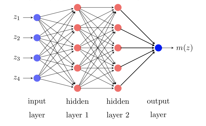
Figure 1: A 3-layer neural network with four input variables and one output.

Note that the total number of parameters in (2) is $\sum_{k=1}^{L}q_{k}(q_{k-1}+1)$, which can be very large and may lead to overfitting. Han et al. (2015); Bauer and Kohler (2019) and Schmidt-Hieber (2020) mitigated against this by deactivating some of the links of neurons between the adjacent hidden layers. Following this strategy, for $s\in\mathbb{N}$, $L\geq 2$, $A>0$ and $\boldsymbol{q}=(q_{0},q_{1},\ldots,q_{L})^{\top}$, we consider a sparsely connected neural network class

$$\mathcal{M}(s,L,\boldsymbol{q},A)=\Big{\{}m(z)= W_{L}\tilde{\sigma}\circ\cdots\circ W_{2}\tilde{\sigma}(W_{1}\tilde{z})~{}|~{}W_{k}\in\mathbb{R}^{q_{k}\times(q_{k-1}+1)},~{}\|W_{k}\|_{\infty}\leq 1~{}\text{for}~{}$$ (3)

$$k=1,\ldots,L,~{}\sum_{k=1}^{L}\|W_{k}\|_{0}\leq s~{}\text{and}~{}\|m\|_{\infty}\leq A\Big{\}},$$

where $\|\cdot\|_{\infty}$ is the sup-norm of a matrix or function and $\|\cdot\|_{0}$ is the number of non-zero elements of a matrix.

2.2 Partially linear quantile regression model and estimation

Consider a univariate random variable $Y$ and a multivariate random variable $U=(X,Z)\in\mathbb{R}^{p}\times\mathbb{R}^{q}$, of which $X$ can include treatment variables and continuous covariates of interest. Let $F_{Y|U}(\cdot|u)$ be the conditional distribution function of $Y$ given $U=u.$ For some $0<\tau<1$, the $\tau$-th conditional quantile of $Y$ given $U=u$ is defined as

$$\xi_{\tau}(u)=\mathop{\inf}_{y\in\mathbb{R}}\{y~{}|~{}F_{Y|U}(y|u)\geq\tau\}.$$

In this paper, we assume $\xi_{\tau}(X,Z)=X^{\top}\theta_{\tau}+m_{\tau}(Z)$, which leads to the following partially linear quantile regression model:

$$Y=X^{\top}\theta_{\tau}+m_{\tau}(Z)+\epsilon,P(\epsilon\leq 0|U)=\tau,$$ (4)

where $\theta_{\tau}\in\mathbb{R}^{p}$ is an unspecified parameter, $m_{\tau}:\mathbb{R}^{q}\rightarrow\mathbb{R}$ is an unknown function and the error $\epsilon$ can be heteroscedastic by allowing it to vary with $u=(x,z)$.

Let $\{(X_{i},Z_{i},Y_{i}):i=1,\ldots,n\}$ denote independent and identically distributed realizations of $(X,Z,Y)$. For simplicity, we use the notation $\mathcal{M}$ to denote the neural network class $\mathcal{M}(s,L,\boldsymbol{q},\infty)$ in (3) with $q_{0}=q$ and $q_{L}=1$. To estimate the vector $\theta_{\tau}$ and the function $m_{\tau}$, we minimize the loss function:

$$(\hat{\theta}_{\tau},\hat{m}_{\tau})=\mathop{\arg\min}_{(\theta,m)\in\mathbb{R}^{p}\times\mathcal{M}}\frac{1}{n}\sum_{i=1}^{n}\rho_{\tau}(Y_{i}-X_{i}^{\top}\theta-m(Z_{i})),$$ (5)

where $\rho_{\tau}(t)=t\{\tau-1(t<0)\}$ is called the check loss. This loss function becomes the absolute value $L^{1}$-loss when $\tau=0.5$ which leads to the median estimators. For brevity, we suppress the subscript $\tau$ and write $(\theta_{0},m_{0})=(\theta_{\tau},m_{\tau})$ and $(\hat{\theta},\hat{m})=(\hat{\theta}_{\tau},\hat{m}_{\tau})$.

3 Theory

In this section, we establish the theoretical properties of the estimators $\hat{\theta}$ and $\hat{m}$. We first introduce a class of smooth functions in which $m_{0}$ resides.

Let $\gamma$ and $B$ be two positive constants and $\lfloor\gamma\rfloor$ denote the largest integer strictly less than $\gamma$. We call a function $h:\mathbb{T}\subset\mathbb{R}^{q}\rightarrow\mathbb{R}$ a $(\gamma,B)$-Hölder smooth function if it satisfies

$$\sup_{z\in\mathbb{T}}\Big{|}\frac{\partial^{|\boldsymbol{\alpha}|}h}{\partial^{\alpha_{1}}z_{1}\ldots\partial^{\alpha_{q}}z_{q}}(z)\Big{|}\leq B,~{}\text{for all}~{}\boldsymbol{\alpha}=(\alpha_{1},\ldots,\alpha_{q})^{\top}\in\mathbb{N}^{q}~{}\text{and}~{}|\boldsymbol{\alpha}|=\sum_{i=1}^{q}\alpha_{i}\leq\lfloor\gamma\rfloor,$$

and

$$\mathop{\sup}_{z,z^{*}\in\mathbb{T}}\Big{|}\frac{\partial^{|\boldsymbol{\alpha}|}h}{\partial^{\alpha_{1}}z_{1}\ldots\partial^{\alpha_{q}}z_{q}}(z)-\frac{\partial^{|\boldsymbol{\alpha}|}h}{\partial^{\alpha_{1}}z_{1}\ldots\partial^{\alpha_{q}}z_{q}}(z^{*})\Big{|}\leq B\|z-z^{*}\|_{2}^{\gamma-\lfloor\gamma\rfloor},~{}\text{for all}~{}|\boldsymbol{\alpha}|=\lfloor\gamma\rfloor.$$

Denote the class of all such $(\gamma,B)$-Hölder smooth functions as $\mathcal{H}_{q}^{\gamma}(\mathbb{T},B)$. Let $J\in\mathbb{N}$, $\boldsymbol{\gamma}=(\gamma_{1},\ldots,\gamma_{J})^{\top}\in\mathbb{R}_{+}^{J}$, $\boldsymbol{d}=(q,d_{1},\ldots,d_{J})^{\top}\in\mathbb{N}^{J+1}$ and $\boldsymbol{\bar{d}}=(\bar{d}_{1},\ldots,\bar{d}_{J})^{\top}\in\mathbb{N}^{J}$ with $\bar{d}_{1}\leq q$ and $\bar{d}_{k}\leq d_{k-1},k=2,\ldots,J$. We further define a composite function class:

$$\mathcal{H}(J,\boldsymbol{\gamma},{\boldsymbol{d}},\boldsymbol{\bar{d}},B)=\Big{\{}h= h_{J}\circ\ldots\circ h_{1}:\mathbb{T}\rightarrow\mathbb{R}~{}|~{}\ h_{k}=(h_{k1},\ldots,h_{kd_{k}})^{\top}~{}\text{and}~{}$$ (6)

$$h_{kj}\in\mathcal{H}_{\bar{d}_{k}}^{\gamma_{k}}([a_{k},b_{k}]^{\bar{d}_{k}},B)~{}\text{for some}~{}|a_{k}|,|b_{k}|\leq B\Big{\}}.$$

Note that this class of functions, first proposed by Schmidt-Hieber (2020), contains two kinds of dimension ${\boldsymbol{d}}$ and $\boldsymbol{\bar{d}}.$ We call $\boldsymbol{\bar{d}}$ the intrinsic dimension of the function $h$ in $\mathcal{H}(J,\boldsymbol{\gamma},{\boldsymbol{d}},\boldsymbol{\bar{d}},B)$.

For an illustration, consider the function

$$h(z)=h_{31}(h_{21}(h_{11}(z_{1},z_{2}),h_{12}(z_{3},z_{4})),h_{22}(h_{13}(z_{5},z_{6}),h_{14}(z_{7}))),$$ (7)

where all $h_{ij}$ are $(\gamma,1)$-Hölder smooth. It is clear that $h\in\mathcal{H}(J,\boldsymbol{\gamma},{\boldsymbol{d}},\boldsymbol{\bar{d}},B)$ with $J=3,\boldsymbol{\gamma}=(\gamma,\gamma,\gamma)^{\top},{\boldsymbol{d}}=(7,4,2,1)^{\top},\boldsymbol{\bar{d}}=(2,2,2)^{\top}$ and $B=1.$

With different choices of $J,\boldsymbol{\gamma},$ ${\boldsymbol{d}}$ and $\boldsymbol{\bar{d}}$, $\mathcal{H}(J,\boldsymbol{\gamma},{\boldsymbol{d}},\boldsymbol{\bar{d}},B)$ includes a large number of function classes that have been considered in the statistical and economic literature. Below we provide two examples to illustrate the ubiquity of such function classes. We say a function $h$ is $(\infty,B)$-Hölder smooth if it is $(\gamma,B)$-Hölder smooth for all $\gamma>0$.

Example 3.1 (Generalize additive functions)

A function $h:\mathbb{R}^{q}\rightarrow\mathbb{R}$ is additive if it can be represented a sum of univariate functions of each components (Stone, 1985), i.e., for $z=(z_{1},\ldots,z_{q})^{\top}$,

$$h(z)=h_{1}(z_{1})+\ldots+h_{q}(z_{q}),$$ (8)

where $h_{k},k=1,\ldots,q$ are univariate $(\gamma,B)$-Hölder smooth functions. Here $J=2,\boldsymbol{\gamma}=(\gamma,\infty)^{\top},$ $\boldsymbol{d}=(q,q,1)^{\top},$ $\boldsymbol{\bar{d}}=(1,q)^{\top},$ $h_{1k}(z)=h_{k}(z_{k}),~{}k=1,\ldots,q$, and $h_{21}(y)=y_{1}+\ldots+y_{q},$ where $y=(y_{1},\ldots,y_{q})^{\top}.$ Furthermore, Horowitz (2001) added an unknown link function $g$ and proposed the generalized additive function:

$$h(z)=g(h_{1}(z_{1})+\ldots+h_{q}(z_{q})),$$

where $g$ and $h_{k},k=1,\ldots,q$ are univariate $(\gamma,B)$-Hölder smooth functions. In this case, the function $h$ has a hierarchical structure with $J=3,\boldsymbol{\gamma}=(\gamma,\infty,\gamma)^{\top},$ $\boldsymbol{d}=(q,q,1,1)^{\top},$ and $\boldsymbol{\bar{d}}=(1,q,1)^{\top},$ $h_{1k}(z)=h_{k}(z_{k}),~{}k=1,\ldots,q$, $h_{21}(y)=y_{1}+\ldots+y_{q},$ for $y=(y_{1},\ldots,y_{q})^{\top},$ and $h_{31}=g.$

Example 3.2 (Single/multiple index functions)

A single index function, first introduced by Ichimura (1993) and later extended to multiple indices by Hristache et al. (2001), is given by :

$$h(z)=h_{1}(z^{\top}\alpha_{1},\ldots,z^{\top}\alpha_{K}),$$ (9)

where $\alpha_{k},k=1,\ldots,K$ are unknown parameters and $z^{\top}\alpha_{j}$ are the index functions. It is easy to see that $h_{1k}(z)=z^{\top}\alpha_{k},k=1,\ldots,K$ and $h_{21}(y)=h_{1}(y)$. Thus, if $h_{1}$ is $(\gamma,B)$-Hölder smooth, $\boldsymbol{\gamma}=(\infty,\gamma)^{\top},$ $\boldsymbol{d}=(q,K,1)^{\top}$ and $\boldsymbol{\bar{d}}=(\bar{d}_{1},K)^{\top}$ with $\bar{d}_{1}=\max_{k}\{\|\alpha_{k}\|_{0}\}.$

For some $J\in\mathbb{N}$, $\boldsymbol{\gamma}=(\gamma_{1},\ldots,\gamma_{J})\in\mathbb{R}_{+}^{J}$, $\boldsymbol{d}=(q,d_{1},\ldots,d_{J})^{\top}\in\mathbb{N}^{J+1}$ and $\boldsymbol{\bar{d}}=(\bar{d}_{1},\ldots,\bar{d}_{J})^{\top}\in\mathbb{N}^{J}$ with $\bar{d}_{1}\leq q$ and $\bar{d}_{k}\leq d_{k-1},k=2,\ldots,J,$ we define the effective smoothness $\bar{\gamma}_{k}=\gamma_{k}\prod_{i=k+1}^{J}(\gamma_{i}\wedge 1)$ of a function $h$ in $\mathcal{H}(J,\boldsymbol{\gamma},{\boldsymbol{d}},\boldsymbol{\bar{d}},B),$ and write

$$\bar{k}=\mathop{\arg\min}_{k\in\{1,\ldots,J\}}\frac{\bar{\gamma}_{k}}{2\bar{\gamma}_{k}+\bar{d}_{k}}~{}\text{and}~{}r_{n}=n^{-\frac{\bar{\gamma}_{\bar{k}}}{2\bar{\gamma}_{\bar{k}}+\bar{d}_{\bar{k}}}}.$$

For the covariate $X=(X_{1},\ldots,X_{p})^{\top}$, we define

$$\varphi_{k}^{*}=\mathop{\arg\min}_{\varphi\in L^{2}(P_{Z})}\mathbb{E}[f(0|U)\{X_{k}-\varphi(Z)\}^{2}],k=1,\ldots,p,$$ (10)

where $L^{2}(P_{Z})=\{\varphi~{}|~{}\mathbb{E}\varphi^{2}(Z)<\infty\}.$ And denote $\boldsymbol{\varphi}^{*}(Z)=(\varphi_{1}^{*}(Z),\ldots,\varphi_{p}^{*}(Z))^{\top},$ $\Sigma_{1}=\mathbb{E}[\tau(1-\tau)\{X-\boldsymbol{\varphi}^{*}(Z)\}\{X-\boldsymbol{\varphi}^{*}(Z)\}^{\top}]$ and $\Sigma_{2}=\mathbb{E}[f(0|U)\{X-\boldsymbol{\varphi}^{*}(Z)\}\{X-\boldsymbol{\varphi}^{*}(Z)\}^{\top}].$ It is easy to show that $\boldsymbol{\varphi}^{*}=\mathbb{E}(X|Z)$, if the conditional error density $f(\cdot|U)$ is independent of $U$ at zero, see also Lian (2012) and Hoshino (2014) for partially linear additive regression.

Next, we state the assumptions for the deep partially linear quantile regression model.

1. The true vector parameter $\theta_{0}$ belongs to a compact subset $\Theta\subset\mathbb{R}^{p}$ and the true nonparametric function $m_{0}$ belongs to $\mathcal{H}=\mathcal{H}(J,\boldsymbol{\gamma},{\boldsymbol{d}},\boldsymbol{\bar{d}},B).$

2. The covariates $(X,Z)$ take values in a compact subset of $\mathcal{R}^{p+q}$ that, without loss of generality, will be assumed to be $[0,1]^{p+q}.$ In addition, the probability density function (PDF) of $Z$ is bounded away from zero and from infinity.

3. The conditional PDF $f(\cdot|u)$ of the random error $\epsilon$ given the covariate $U=u$, has continuous derivative $f^{{}^{\prime}}(\cdot|u),$ and there exist positive constants $b_{0}$ and $c_{0}$ such that $1/c_{0}<f(t|u)<c_{0}$ and $|f^{{}^{\prime}}(t|u)|<c_{0}$ for all $|t|\leq b_{0},u\in[0,1]^{p+q}.$

4. $L=O(\log n),$ $s=O(nr_{n}^{2}\log n)$ and $nr_{n}^{2}\lesssim\text{min}_{k=1,\ldots,L}\{q_{k}\}\leq\text{max}_{k=1,\ldots,L}\{q_{k}\}\lesssim n.$

5. The matrices $\Sigma_{1}$ and $\Sigma_{2}$ are both positive definite.

6. $\bar{\gamma}_{\bar{k}}>\bar{d}_{\bar{k}}/2$ and $\max_{k=1,\ldots,p}(\mathbb{E}|X_{k}|^{4})<\infty.$

The boundedness of both the parameters and covariate spaces in assumptions (A1) and (A2) are standard for semiparametric/nonparametric regression. In (A3) we assume that the PDF of the error and its derivative are bounded to guarantee that the true parameter $(\theta_{0},m_{0})$ is a well-separated point of the minimum of the expected check loss function. For (A4), we assume that the size of neural networks $\mathcal{M}$ used in (5) grows with the sample size $n$ at a certain rate to balance the approximation and estimation errors of the estimators. Assumptions (A5) and (A6) are common conditions for asymptotic normality of the vector estimator $\hat{\theta}$ in semiparametric regression (Horowitz, 2009), where (A5) is used to develop the asymptotic variance while (A6) guarantees $\sqrt{n}$-consistency.

We are now ready to state the convergence rate of the estimators.

Theorem 3.1

Under Assumptions (A1)-(A5), we have

$$\lim_{C\rightarrow\infty}\lim_{n\rightarrow\infty}\sup_{m_{0}\in\mathcal{H}}\mathbb{P}(\|\hat{m}-m_{0}\|_{L^{2}([0,1]^{q})}\geq Cr_{n}\log^{2}n)=0.$$

From the proof of Theorem 3.1 one can see that the convergence rate is the result of a trade-off between estimation error and approximation error. Here the approximation error is defined as the distance between the true parameter $m_{0}$ and the neural network set $\mathcal{M},$ i.e., $\mathop{\min}_{m\in\mathcal{M}}\|m-m_{0}\|_{L^{2}([0,1]^{q})}$. It is known that a more complex neural network structure is more flexible and thus leads to a smaller approximation error (Anthony and Bartlett, 1999; Yarotsky, 2017; Bauer and Kohler, 2019; Schmidt-Hieber, 2020). However, too many parameters will lead to high variance. Hence, there is an implicit “bias-variance” trade-off that is reflected in the growth of neural networks.

Note that the convergence rate of the estimator $\hat{m}$ is determined by both the effective smoothness and the intrinsic dimension of the true function $m_{0}$, rather than the dimension $q$ of the covariate $Z$. For example, if $m_{0}$ has the composite structure in (7), the convergence rate for the proposed method is $n^{-\gamma/(2\gamma+2)}\log^{2}n$. In contrast, the convergence rate for a nonparametric method, such as kernel or spline smoothing is of the order $n^{-\gamma/(2\gamma+7)}$. This shows that our method is able to detect the low dimensional structure of the data and circumvents the curse of dimensionality.

In particular, when $m_{0}$ reduces to additive or single index function, the resulting estimators have one-dimensional nonparametric rates of convergence (up to a poly-logarithmic factor). This is similar to results of Stone (1985) and Ichimura (1993) for nonparametric regression.

The next theorem establishes the minimax lower bound for estimating $m_{0}$, which implies that the resulting estimator $\hat{m}$ in Theorem 3.1 is rate-optimal.

Theorem 3.2

Let $\mathcal{F}$ be the class of probability density functions that satisfy Assumption (A3). Then we have

$$\mathop{\lim}_{C\rightarrow\infty}\mathop{\lim}_{n\rightarrow\infty}\mathop{\inf}_{\hat{m}}\mathop{\sup}_{(\theta_{0},m_{0},f)\in\mathbb{R}^{q}\times\mathcal{H}\times\mathcal{F}}\mathbb{P}_{(\theta_{0},m_{0},f)}\big{(}\|\hat{m}-m_{0}\|_{L^{2}([0,1]^{q})}\geq Cr_{n}\big{)}=1,$$

where the infimum is taken over all possible predictors $\hat{m}$ based on the observed data.

Below we show that the estimator $\hat{\theta}$ for the vector parameter is asymptotically normal at the $\sqrt{n}$ rate.

Theorem 3.3

Under Assumptions (A1)-(A6), we have

$$\sqrt{n}(\hat{\theta}-\theta_{0})\rightarrow N(0,\Sigma_{2}^{-1}\Sigma_{1}\Sigma_{2}^{-1}).$$

When $f(0|U)$ is a constant function, the solution of (10) would be $\boldsymbol{\varphi}^{*}(Z)=\mathbb{E}(X|Z),$ which leads to $\Sigma_{1}=\tau(1-\tau)\text{Var}\{X-\mathbb{E}(X|Z)\}$, $\Sigma_{2}=f(0)\text{Var}\{X-\mathbb{E}(X|Z)\}$ and more generally, the following corollary.

Corollary 3.1

Under the same assumptions of Theorem 3.3 and when $f(0|U)$ is a constant function, we have

$$\sqrt{n}(\hat{\theta}-\theta_{0})\rightarrow N(0,\Sigma),$$

where $\Sigma={\tau(1-\tau)}[\text{Var}\{X-\mathbb{E}(X|Z)\}]^{-1}/{f^{2}(0)}.$

For partially linear quantile regression with homoscedastic error, the random error $\epsilon$ is independent of the covariate $U$, which implies that $f(0|U=u)=f(0),$ for all $u\in[0,1]^{p+q}$, hence Corollary 3.1 holds.

4 Implementation and Asymptotic Covariance

Estimations of $\hat{\theta}$ and $\hat{m}$: Since the check loss function in (5) is not differentialable at the origin, the Newton-Raphson algorithm and its variants cannot be directly used to find the solution for linear quantile regression. Koenker and Ng (2005) proposed several algorithms, such as the interior point algorithm for linear programming, to solve this optimization problem. However, with the layer-by-layer structure of the neural network and the large number of parameters involved, this approach is infeasible for our purpose. We resort to the Adam algorithm (Kingma and Ba, 2014), a variant of the stochastic gradient descent (Robbins and Monro, 1951), in the R package Keras to solve the optimization problem (5). This algorithm is widely used in the deep learning field due to its computational and memory efficiency. For our purpose, since we have a parametric and a nonparametric component, we wrap the linear predictor $\theta^{\top}X$ and $m(Z)$ together and iteratively estimate the corresponding parameters simultaneously. That is, with the neural network $m$ in (2), we use Adam to update the parameters $\{\theta,W_{1},\ldots,W_{L}\}.$ Here we use the default values in Keras for the initial values $\theta^{(0)}$ and $W_{k}^{(0)},k=1,\ldots,L$.

The algorithm also requires the specification of tuning parameters, such as the depth $L$, width $\boldsymbol{q}$, step size, minibatch size, the number of iterations and early stopping. Here the minibatch size is defined as the subsample size used to calculate the gradient of the objective function for each iteration, and early stopping prevents overfitting by specifying the number of iterations to continue when the model does not improve any more on a hold-out validation dataset. We first hold out 20% of the training data to select the tuning parameters among a large number of candidates, and then use the selected tuning parameters to redo estimation on the earlier training dataset. Table 11 below shows the resulting selected tuning parameters that are used for the numerical studies in this paper.

Asymptotic Covariance Estimation:  To obtain inference for the parameter $\theta_{0}$, we need to estimate the asymptotic covariance matrix of $\hat{\theta}$ in Theorem 3.3 or Corollary 3.1. For simplicity, we demonstrate how to estimate the asymptotic covariance matrix for the case of homoscedastic random errors. The first step is to obtain a density estimate for $\hat{f}(0)$ from the residuals $\{\hat{\epsilon}_{i}=Y_{i}-\hat{Y}_{i}~{}|~{}\hat{Y}_{i}=X_{i}^{\top}\hat{\theta}+\hat{m}(Z_{i}),i=1,\ldots,n\},$ for which we use density in the R package stats. Then, we employ the deep neural network to estimate the projections ${\varphi}^{*}_{k},k=1,\ldots,p$ empirically, that is,

$$\hat{\varphi}^{*}_{k}=\mathop{\arg\min}_{\varphi\in\mathcal{M}_{1}}\frac{1}{n}\sum_{i=1}^{n}\{X_{ik}-\varphi(Z_{i})\}^{2},$$

where $X_{ik}$ is the $k$-th component of covariates $X_{k}$ and $\mathcal{M}_{1}$ is a class of neural networks. Let $\boldsymbol{\hat{\varphi}}^{*}=(\hat{\varphi}^{*}_{1},\ldots,\hat{\varphi}^{*}_{p})^{\top},$ $V_{i}=X_{i}-\boldsymbol{\hat{\varphi}}^{*}(Z_{i})$, $\bar{V}=1/n\sum_{i=1}^{n}V_{i}$, and

$$\hat{\Omega}=\frac{1}{n-1}\sum_{i=1}^{n}(V_{i}-\bar{V})(V_{i}-\bar{V})^{\top}.$$

Finally, we estimate the asymptotic covariance matrix by

$$\hat{\Sigma}=\frac{\tau(1-\tau)\hat{\Omega}^{-1}}{\hat{f}^{2}(0)}.$$

For heteroscedastic random errors, we can estimate the corresponding asymptotic covariance matrix by a bootstrap method, see Feng et al. (2011) and Wang et al. (2018) for details.

5 Simulations

In this section, we demonstrate the numerical performance of the proposed deep quantile regression method and compare it with linear quantile regression and partially linear additive quantile regression, abbreviated as LQR and PLAQR, respectively. LQR and PLAQR were implemented with the R packages quantreg and plaqr, which are publicly available at https://cran.r-project.org/package=quantreg and https://cran.r-project.org/package=plaqr, respectively.

5.1 Simulation I: Homoscedastic Errors

We first generated $\tilde{Z}=(\tilde{Z}_{1},\ldots,\tilde{Z}_{12})^{\top}$ from a Gaussian copula on $[0,2]$ with correlation parameter $0.5$. Marginally, each coordinate of $\tilde{Z}$ is a uniform distribution on $[0,2]$. We then set $Z=(\tilde{Z}_{1},\ldots,\tilde{Z}_{10})^{\top}$ and $X=(X_{1},X_{2})^{\top}$ with $X_{1}=1(\tilde{Z}_{11}>1)$ and $X_{2}=\tilde{Z}_{12}$ as covariates. The response $Y$ was generated from

$$Y=\theta^{\top}X+m(Z)+\epsilon,$$ (11)

where $\theta=(\theta_{1},\theta_{2})=(1,-1)^{\top}$, and the error $\epsilon,$ independent of $(X,Z),$ is a Student’s t-distribution with zero mean and $3$ degrees of freedom. Three choices of $m$ were implemented:

1. (linear): $m(z)=0.95\times\sum_{k=1}^{10}z_{k}$;

2. (additive): $m(z)=1.1\times\{z_{1}^{3}-3z_{2}^{2}+2\sin(6\pi z_{3})+\log(z_{4}+0.5)+\sqrt{z_{5}+2}+e^{z_{6}/2}+0.5(z_{7}-1+|z_{7}-1|)+{1}/{(z_{8}+2)}+2e^{-z_{9}/2}+\cos(\pi z_{10})\}$;

3. (deep): $m(z)=0.51\times[z_{1}z_{2}+z_{2}\{1-\cos(\pi z_{3}z_{4})\}+{2\sin(z_{5})}/{(|z_{5}-z_{6}|+2)}+(z_{6}+z_{7}z_{8}-1)^{2}+\sqrt{z_{9}^{2}+z_{10}^{2}+2}+\exp\{{\sum_{k=1}^{10}(z_{k}-1)}/{5}\}].$

The first two cases correspond to, respectively, the LQR and PLAQR model, and the third case is designed for DPLQR. The factors $0.95,1.1$ and $0.51$ in each case were scaled to attain a signal-to-noise ratio around $5$.

For each setting, we generated $Q=160$ datasets with respective sample sizes $n=500$ and $2000$ in each dataset. Throughout the simulation, we split the data into training data and testing data in a 80:20 ratio. That is, 80% of the data were used for estimation (including 20% for tuning) as introduced in Section 4, while 20% for evaluating the resulting estimates (test data). The performance of $\hat{m}_{\tau}$ was assessed by the relative mean squared error (RMSE):

$$RMSE(\hat{m}_{\tau})=\frac{\frac{1}{N}\sum_{i=1}^{N}\{\hat{m}_{\tau}(Z_{i})-m_{\tau}(Z_{i})\}^{2}}{\frac{1}{N}\sum_{i=1}^{N}\{m_{\tau}(Z_{i})\}^{2}},$$ (12)

where $\hat{m}_{\tau}$ and $m_{\tau}$ are evaluated on the covariates $Z_{i},i=1,\ldots,N$ of the test data. Moreover, with the estimates $\hat{\theta}_{\tau}$ and $\hat{m}_{\tau}$, we use $\hat{Y}_{i}=X_{i}^{\top}\hat{\theta}_{\tau}+\hat{m}_{\tau}(Z_{i})$ to predict $Y_{i}$ and evaluated its performance through the mean squared prediction error:

$$MSPE(\hat{y})=\frac{1}{N}\sum_{i=1}^{N}(\hat{Y}_{i}-Y_{i})^{2}.$$

Here the prediction is also evaluated on the test data.

Table 1 presents the biases and standard deviations of the estimates, $\hat{\theta}=(\hat{\theta}_{1},\hat{\theta}_{2})$, based on 160 simulation runs at three quantile levels $\tau=0.2,0.5,0.8$. In general, both the bias and variance decrease steadily for all three methods as the sample size increases from 500 to 2000. As expected, the mean squared error of the resulting estimates are the smallest at the median ($\tau=0.5$) level. Under Case 1 (linear) and Case 2 (additive), the proposed DPLOR method performed comparably with the optimal method (LQR and PLAQR respectively) with slightly larger mean squared errors. However, under Case 3 (deep), the DPLQR method clearly outperforms LQR and PLAQR. We also construct the $95\%$ confidence intervals for $\theta_{1}$ and $\theta_{2}$ based on the estimates of the asymptotic variance in Section 4. Table 2 reports the empirical coverage probabilities of the 95% confidence intervals. For all three cases, the empirical coverage probabilities of the proposed method generally approach $95\%$ as $n$ increases. Moreover, the proposed method is comparable to the other two methods under Case 1 (linear) and Case 2 (additive), and has more accurate coverage rates under Case 3 (deep).

The average relative mean squared errors of the estimated nonparametric function $\hat{m}$ over $160$ repetitions are given in Table 3. They decline with the sample sizes as expected. When the true model is Case 3 (deep), the proposed method substantially outperforms LQR and PLAQR, while it performs slightly worse under Case 1 (linear) and Case 2 (additive).

Table 4 shows the mean of the squared predicted errors of the predicted value $\hat{Y}$ based on the median ($\tau=0.5$) regression and reveals that the proposed DPLQR is competitive with the optimal procedure (LQR in Case 1 and PLAQR in Case 2) and superior in Case 3.

Table 1: Bias and standard deviation (in parentheses) of $\hat{\theta}$ for the LQR, PLAQR and DPLQR methods under homoscedastic random errors.

$\tau=0.2$ $\tau=0.5$ $\tau=0.8$ Case $n$ LQR PLAQR DPLQR LQR PLAQR DPLQR LQR PLAQR DPLQR $\theta_{1}$ Case 1 500 0.0068 -0.0053 0.0169 0.0027 -0.0087 0.0109 -0.0262 -0.0239 -0.0743 (linear) (0.1853) (0.1873) (0.1848) (0.1611) (0.1618) (0.1602) (0.2564) (0.2787) (0.2806) 2000 -0.0046 0.0048 0.0145 0.0028 0.0019 0.0160 0.0208 0.0164 0.0454 (0.0932) (0.0940) (0.0927) (0.0815) (0.0827) (0.0810) (0.1388) (0.1455) (0.1442) Case 2 500 0.0086 0.0079 -0.0182 0.0021 0.0108 -0.0422 0.0816 0.0088 -0.0831 (additive) (0.3890) (0.3309) (0.3333) (0.4140) (0.3686) (0.3781) (0.4891) (0.4744) (0.4758) 2000 -0.0272 -0.0088 -0.0012 0.0018 0.0059 0.0017 0.0523 0.0050 0.0477 (0.2136) (0.1637) (0.1680) (0.2116) (0.1889) (0.1925) (0.2517) (0.2343) (0.2408) Case 3 500 0.0099 0.0244 0.0180 -0.0039 -0.0493 0.0066 -0.4256 -0.0016 -0.0497 (deep) (0.2900) (0.2674) (0.1919) (0.2882) (0.2618) (0.1839) (1.2277) (0.4148) (0.3176) 2000 -0.0166 -0.0144 0.0057 0.0106 -0.0160 0.0135 -0.4222 -0.0434 -0.0056 (0.1517) (0.1414) (0.0968) (0.1402) (0.1382) (0.0892) (0.7151) (0.2260) (0.1381) $\theta_{2}$ Case 1 500 -0.0135 -0.0236 0.0357 0.0109 0.0191 0.0321 -0.0530 -0.0483 0.2028 (linear) (0.1880) (0.1952) (0.1977) (0.1605) (0.1701) (0.1634) (0.3390) (0.3444) (0.3976) 2000 -0.0021 -0.0056 0.0182 0.0087 0.0093 0.0180 0.0003 -0.0045 0.0952 (0.0882) (0.0904) (0.0930) (0.0749) (0.0775) (0.0787) (0.1641) (0.1665) (0.1678) Case 2 500 0.0033 0.0021 0.0135 0.0369 -0.0117 0.0258 -0.0140 0.0426 0.1427 (additive) (0.3274) (0.2639) (0.2813) (0.4024) (0.3750) (0.3785) (0.6286) (0.6140) (0.4951) 2000 -0.0020 -0.0011 0.0052 -0.0048 -0.036 -0.0042 0.0185 0.0072 0.0121 (0.1800) (0.1329) (0.1358) (0.2096) (0.2033) (0.2075) (0.2782) (0.2473) (0.2468) Case 3 500 -0.0216 -0.0332 0.0387 -0.0011 -0.0282 0.0802 0.0535 0.0242 0.2552 (deep) (0.2886) (0.2561) (0.1893) (0.2955) (0.2592) (0.1856) (1.0797) (0.3909) (0.3088) 2000 -0.0035 -0.0058 0.0171 -0.0064 -0.0127 0.0244 0.0425 -0.0198 0.0814 (0.1523) (0.1384) (0.0887) (0.1695) (0.1292) (0.0935) (0.5007) (0.2013) (0.1607)

Table 2: Empirical coverage probability of the 95% confidence interval for $\theta=(\theta_{1},\theta_{2})$ by the LQR, PLAQR and DPLQR methods under homoscedastic random errors.

$\tau=0.2$ $\tau=0.5$ $\tau=0.8$ Case $n$ LQR PLAQR DPLQR LQR PLAQR DPLQR LQR PLAQR DPLQR $\theta_{1}$ Case 1 500 0.9500 0.9125 0.9750 0.9188 0.8875 0.9688 0.9188 0.9125 0.9750 (linear) 2000 0.9625 0.9312 0.9688 0.9500 0.9312 0.9625 0.9312 0.9250 0.9625 Case 2 500 0.9000 0.9062 0.9812 0.9125 0.8750 0.9688 0.9062 0.8875 0.9688 (additive) 2000 0.8938 0.9250 0.9688 0.9125 0.9375 0.9125 0.8438 0.9375 0.9625 Case 3 500 0.8750 0.9250 0.9125 0.8875 0.8750 0.9375 0.9688 0.8938 0.8812 (deep) 2000 0.9312 0.8750 0.9375 0.9688 0.8688 0.9562 0.5062 0.8938 0.9438 $\theta_{2}$ Case 1 500 0.9312 0.8812 0.9250 0.8938 0.9188 0.9250 0.9062 0.8938 0.8063 (linear) 2000 0.9375 0.9312 0.9375 0.9500 0.9188 0.9625 0.9100 0.062 0.9000 Case 2 500 0.8938 0.9375 0.9688 0.8688 0.8875 0.9125 0.8500 0.9312 0.8875 (additive) 2000 0.8750 0.9438 0.9562 0.8562 0.9375 0.9125 0.8875 0.9438 0.8938 Case 3 500 0.8938 0.9062 0.9125 0.8812 0.8875 0.9125 0.9500 0.8938 0.8250 (deep) 2000 0.9062 0.8688 0.9375 0.9688 0.8688 0.9312 0.8000 0.8875 0.9250

Table 3: Relative mean squared error of $\hat{m}$ for the LQR, PLAQR and DPLQR methods under homoscedastic random errors.

$\tau=0.2$ $\tau=0.5$ $\tau=0.8$ Case $n$ LQR PLAQR DPLQR LQR PLAQR DPLQR LQR PLAQR DPLQR Case 1 500 0.0019 0.0045 0.0037 0.0009 0.0020 0.0018 0.0021 0.0037 0.0049 (linear) 2000 0.0004 0.0010 0.0009 0.0002 0.0004 0.0004 0.0005 0.0008 0.0010 Case 2 500 0.2650 0.1560 0.2361 0.2176 0.1503 0.1962 0.2492 0.2018 0.2199 (additive) 2000 0.2518 0.1362 0.1596 0.1937 0.1175 0.1347 0.2202 0.1647 0.1811 Case 3 500 0.1307 0.1188 0.0796 0.0955 0.0345 0.0183 0.1464 0.0152 0.0132 (deep) 2000 0.1244 0.0996 0.0232 0.0899 0.0258 0.0087 0.1160 0.0080 0.0053

Table 4: Mean of the squared prediction errors evaluated on the test set for the LQR, PLAQR and DPLQR methods under homoscedastic random errors.

Case $n$ LQR PLAQR DPLQR Case 1 500 3.1028 3.1948 3.1774 (linear) 2000 2.9302 2.9545 2.9484 Case 2 500 8.1803 6.8469 7.1238 (additive) 2000 7.8553 6.1522 6.3471 Case 3 500 6.9982 4.6561 3.8578 (deep) 2000 6.3220 3.9613 3.1862

Table 5: Bias and standard deviation (in parentheses) of $\hat{\theta}$ for the LQR, PLAQR and DPLQR methods under heteroscedastic random errors.

$\tau=0.2$ $\tau=0.5$ $\tau=0.8$ Case $n$ LQR PLAQR DPLQR LQR PLAQR DPLQR LQR PLAQR DPLQR $\theta_{1}$ Case 4 500 0.0351 0.0459 0.0525 -0.0127 0.0037 0.0051 0.0693 0.0960 -0.1815 (linear) (0.4054) (0.4443) (0.4042) (0.3070) (0.3240) (0.3102) (0.5661) (0.6115) (0.5699) 2000 -0.0332 -0.0436 0.0085 -0.0166 -0.0089 0.0130 0.0005 0.0040 0.0294 (0.2254) (0.2414) (0.2249) (0.1736) (0.1837) (0.1779) (0.2866) (0.3095) (0.2908) Case 5 500 0.0437 0.0785 -0.0302 0.0058 0.0203 -0.0671 0.0855 -0.1677 -0.2673 (additive) (0.5168) (0.4704) (0.4799) (0.5006) (0.4305) (0.4435) (0.7398) (0.7104) (0.7271) 2000 0.1465 0.1086 0.1424 -0.0041 -0.0180 0.0027 0.1163 -0.1208 -0.0729 (0.2750) (0.2437) (0.2452) (0.2547) (0.2253) (0.2292) (0.3699) (0.3562) (0.3625) Case 6 500 0.0511 0.0346 0.0494 0.0784 -0.0472 -0.0160 1.4354 -0.0252 -0.0695 (deep) (0.5284) (0.4786) (0.3563) (0.4040) (0.3829) (0.2911) (1.4179) (0.6577) (0.4847) 2000 0.0629 0.0484 0.0230 0.0910 -0.0203 0.0054 1.6135 -0.0159 -0.0022 (0.2613) (0.2353) (0.1842) (0.2188) (0.1872) (0.1354) (0.6215) (0.3223) (0.2313) $\theta_{2}$ Case 4 500 -0.0507 -0.0483 0.1967 -0.0111 -0.0066 0.2677 -0.0094 0.0116 0.3887 (linear) (0.3678) (0.3695) (0.3688) (0.3234) (0.3300) (0.3346) (0.6264) (0.6352) (0.6381) 2000 0.0101 0.0097 0.0663 0.0071 0.0048 0.0607 -0.0538 -0.0400 0.1558 (0.1846) (0.1875) (0.1861) (0.1541) (0.1617) (0.1592) (0.2958) (0.2919) (0.3009) Case 5 500 0.0660 0.0851 0.1920 -0.0376 -0.0237 0.0064 -0.1001 -0.1008 0.2185 (additive) (0.4954) (0.4484) (0.4570) (0.5132) (0.4182) (0.4200) (0.8267) (0.7533) (0.8010) 2000 0.0680 0.0712 0.0854 -0.0034 -0.0060 0.0087 -0.1277 -0.1116 -0.0383 (0.2565) (0.2150) (0.2186) (0.2755) (0.2083) (0.2125) (0.3939) (0.3686) (0.3767) Case 6 500 0.0645 0.0987 0.0772 0.0697 0.0156 0.0865 0.0120 -0.0711 0.2220 (deep) (0.4301) (0.3816) (0.2843) (0.3965) (0.3673) (0.2504) (0.9971) (0.5929) (0.3597) 2000 0.0414 0.0302 0.0285 0.0489 -0.0179 0.0207 -0.0721 -0.0335 0.0931 (0.2253) (0.1993) (0.1391) (0.1917) (0.1838) (0.1187) (0.4851) (0.3062) (0.1686)

Table 6: Empirical coverage probability of the 95% confidence interval for $\theta=(\theta_{1},\theta_{2})$ by the LQR, PLAQR and DPLQR methods under heteroscedastic random errors.

$\tau=0.2$ $\tau=0.5$ $\tau=0.8$ Case $n$ LQR PLAQR DPLQR LQR PLAQR DPLQR LQR PLAQR DPLQR $\theta_{1}$ Case 4 500 0.9188 0.9188 0.9125 0.9125 0.9562 0.9750 0.9125 0.8875 0.8688 (linear) 2000 0.9375 0.9188 0.9250 0.9562 0.9250 0.9188 0.9375 0.8938 0.9125 Case 5 500 0.8878 0.9062 0.9625 0.8812 0.8878 0.8812 0.8625 0.9250 0.9750 (additive) 2000 0.9125 0.9375 0.9250 0.9062 0.9250 0.9125 0.8250 0.9562 0.9375 Case 6 500 0.8875 0.8750 0.8938 0.9000 0.8625 0.9188 0.9062 0.8625 0.9062 (deep) 2000 0.9063 0.8938 0.9250 0.8875 0.8875 0.9188 0.8750 0.9188 0.9250 $\theta_{2}$ Case 4 500 0.8812 0.8750 0.8938 0.8688 0.8812 0.8625 0.8812 0.9125 0.8750 (linear) 2000 0.9188 0.9062 0.9062 0.9375 0.9125 0.9062 0.9312 0.9250 0.9125 Case 5 500 0.8750 0.9125 0.9062 0.9000 0.9125 0.8750 0.8875 0.8875 0.8750 (additive) 2000 0.8312 0.9125 0.9125 0.8620 0.9312 0.9250 0.9000 0.9125 0.9062 Case 6 500 0.9062 0.8875 0.9125 0.8750 0.9000 0.9000 0.9250 0.9250 0.8812 (deep) 2000 0.8875 0.8688 0.9188 0.8625 0.8688 0.9250 0.8500 0.8562 0.9125

Table 7: Relative mean squared error of $\hat{m}$ for the LQR, PLAQR and DPLQR methods under heteroscedastic random errors.

$\tau=0.2$ $\tau=0.5$ $\tau=0.8$ Case $n$ LQR PLAQR DPLQR LQR PLAQR DPLQR LQR PLAQR DPLQR Case 4 500 0.0108 0.0276 0.0199 0.0032 0.0089 0.0062 0.0058 0.0145 0.0103 (linear) 2000 0.0026 0.0063 0.0050 0.0009 0.0021 0.0016 0.0012 0.0029 0.0026 Case 5 500 0.2799 0.2075 0.2241 0.2306 0.1796 0.2034 0.2679 0.2206 0.2296 (additive) 2000 0.2514 0.1432 0.1716 0.1948 0.1232 0.1440 0.1791 0.1389 0.1492 Case 6 500 0.2830 0.2362 0.1895 0.1086 0.0685 0.0329 0.1098 0.0308 0.0187 (deep) 2000 0.1876 0.1450 0.0697 0.0908 0.0388 0.0186 0.0865 0.0157 0.0072

Table 8: Mean of the squared prediction errors evaluated on the test set for the LQR, PLAQR and DPLQR methods under heteroscedastic random errors.

Case $n$ LQR PLAQR DPLQR Case 4 500 18.0770 18.7186 18.3779 (linear) 2000 17.8294 17.9436 17.9470 Case 5 500 21.8791 19.9281 20.5156 (additive) 2000 21.6721 19.8431 20.0425 Case 6 500 18.5553 17.0905 16.0694 (deep) 2000 18.4154 16.8250 15.7411

5.2 Simulation II: Heteroscedastic Errors

We also studied the performance of the proposed method for heteroscedastic errors. The covariates $U=(X,Z)$, coefficient $\theta$ and nonparametric function $m$ are similar to the settings in Section 5.1 but the response $Y$ now comes from the regression model:

$$Y=X^{\top}\theta+m(Z)+\sigma_{1}(X,Z)\epsilon.$$

Here $\epsilon$ follows the Student’s t-distribution with zero mean and 3 degrees of freedom. The function $\sigma_{1}(X,Z)$ has the following three settings:

1. 4 (linear): $\sigma_{1}(x,z)=(x_{1}+x_{1}+\sum_{k=1}^{10}z_{k})/5;$

2. 5 (additive): $\sigma_{1}(x,z)=(x_{1}+x_{1}+\sum_{k=1}^{10}|z_{k}-0.2|)/3.6;$

1. $\sigma_{1}(x,z)=(x_{1}+x_{1})/3+3\Phi\big{(}{\sum_{k=1}^{10}(z_{k}-1)}/{5}\big{)}$ with the cumulative distribution function $\Phi(\cdot)$ of the standard normal distribution.

These lead to $\theta_{\tau}=\theta+t_{\tau}\theta^{*}$ and $m_{\tau}(z)=m(z)+t_{\tau}m^{*}(z)$ with $t_{\tau}$ being the $\tau$ quantile of Student’s t-distribution with zero mean and degree of freedom 3. The simulation results, which are summarized in Table 5 - Table 8, are comparable to those in Simulation I in Section 5.1.

In summary, when the true model is linear or partially linear additive quantile regression, our method is competitive for both the parametric coefficients and nonparametric function estimates, and the coverage probabilities for the parametric coefficients are close to the 95% nominal level as sample sizes increase. Furthermore, the proposed method is superior to the LQR and PLAQR methods when the true model comes from the deep partially linear quantile regression.

6 Applications to Real Data

6.1 Concrete Compressive Strength Data

We apply the proposed methodology, along with the competing methods, to the Concrete Compressive Strength Data Set (Yeh, 1998) available on the UCI machine learning repository. The data consist of $n=1030$ observations, with the response being a continuous variable of concrete compressive strength (CCS), and eight covariates: $Z_{1}$(cement), $Z_{2}$(water), $Z_{3}$(fly ash), $Z_{4}$(blast furnace slag), $Z_{5}$(superplasticizer), $Z_{6}$(coarse aggregate), $Z_{7}$(fine aggregate) and $Z_{8}$(age of the mixture in days), of which the first seventh covariates are the ingredients in high-performance concrete (HPC). For concrete technology, the water-cement ratios (WCR) has been recognized as the most useful and significant advancement for CCS (Yeh, 1998). Here we not only explore the association between WCR and CCS, but also predict the CCS of HPC from the covariates.

As in the simulations, we model the data with four approaches: (a) the proposed deep partially linear quantile regression (DPLQR), (b) linear quantile regression (LQR), (c) partially linear additive quantile regression (PLAQR), and (d) deep nonparametric quantile regression (DNQR, see Jantre et al. (2020); Padilla et al. (2020)). Note that model (d) does not offer direct treatment effects.

For the data, we treat log CCS as the response, WCR, i.e, $Z_{2}/Z_{1}$, as the linear predictors $X$, and $(Z_{3},Z_{4},Z_{5},Z_{6},Z_{7},Z_{8})^{\top}$ as the predictors $Z$ in models (a), (b) and (c). In model (d), we nonparametriclly regress response log CCS on all covariates $(Z_{1},\ldots,Z_{8})$ and implement it via deep learning. We use 80% of the data to train and tune the model and hold out the rest 20% of data to assess the prediction performance of the four methods.

Table 9 shows the numerical results at the median level ($\tau=0.5$). The 95% confidence interval for $\theta$ of each method suggests that there is a strong association between WCR and CCS. The negative estimates further support the Abrams rule in civil engineering that increase in the WCR tends to decrease the strength of concrete (Gorse et al., 2012). Among the first three approaches, DPLQR produced a shorter 95% confidence interval for $\theta$ than the LQR and PLAQR methods. The prediction results in Table 9 further reveal that our method not only improves the prediction accuracy substantially but also has the smallest standard deviation. Although the proposed model is a submodel of the DNQR in (d), its performance in prediction is comparable. Thus, compared to the fully nonparametric approach (d), the partially linear approach (c) trades a small amount of prediction accuracy for interpretibility and has the best performance among the three interpretable approaches (a)-(c).

Table 9: Estimation and prediction results for the Concrete Compressive Strength Data. CI: confidence interval; MEAN: mean of the squared prediction errors; SD: standard deviation of the squared prediction errors.

Estimation Prediction error $\hat{\theta}$ 95% CI MEAN SD LQR -1.3043 [-1.4803, -1.2147] 0.1718 0.2557 PLAQR -1.0959 [-1.2718, -1.0241] 0.0708 0.1080 DPLQR -1.2627 [-1.3248, -1.2006] 0.0319 0.0740 DNQR - - 0.0308 0.0615

6.2 Boston Housing Data

The Boston Housing Data, available from the R package mlbench, is a benchmark dataset for quantile regression analysis. In Harrison and Rubinfeld (1978), 506 observations were examined to study the housing prices based on various demographic and socioeconomic predictors. The variables are: $Y$ (median hoouse price), $X_{1}$ (per capita crime rate by town), $X_{2}$ (a river boundary indicator), $X_{3}$ (proportion of non-retail business acres per town), $X_{4}$ (proportion of residential land zoned for lots), $X_{5}$ (nitrogen oxides concentration), $X_{6}$ (average number of rooms per dwelling), $X_{7}$ (proportion of owner-occupied units built prior to 1940), $X_{8}$ (weighted mean of distances to five Boston employment centers), $X_{9}$ (index of accessibility to radial highways), $X_{10}$ (full-value property-tax rate), $X_{11}$ (pupil-teacher ratio by town), $X_{12}$ (the proportion of black individuals by town), $X_{13}$ (the percentage of the population classified as lower status).

To study the effect of the crime rate on house price, we choose $X_{1}$ (per capita crime rate by town) and the binary coavriate $X_{2}$ (a river boundary indicator) as the vector predictors and all other continuous covariates as the nonparametric predictors.

$$\log Y=\theta_{1}X_{1}+\theta_{2}X_{2}+m(X_{3},\ldots,X_{13})+\epsilon.$$

Here the function $m$ is modelled as a linear, additive and nonparametric function, which corresponds to the LQR, PLAQR and DPLQR models, respectively. We also include the DNQR method, which treats all thirteen covariates as components of a nonparametric regression model, i.e. $\log Y=m(X_{1},X_{2},X_{3},\ldots,X_{13})+\epsilon.$

The estimates $\hat{\theta}_{1}$ from the median regression are summarized in Table 10, revealing that the crime rate has a significant effect on the price of a house and house prices are higher in areas with lower crime rates. Table 10 also displays the mean and standard deviation of squared prediction errors ( hold-out 20% as test set). The proposed method is considerably better than the LQR and PLADR methods. Furthermore, we note that the DNQR method leads to a larger squared prediction error than our method.

Table 10: Estimation and prediction results for the Boston Housing Data. CI: confidence interval; MSPE: mean of the squared prediction errors; SD: standard deviation of the squared prediction errors.

Estimation Prediction $\hat{\theta}_{1}$ 95% CI MEAN SD LQ -0.0093 [-0.0274, -0.0081] 0.0799 0.2048 PLAQR -0.0112 [-0.0309, -0.0082] 0.0529 0.1314 DPLQR -0.0117 [-0.0137, -0.0096] 0.0272 0.0559 DNQR - - 0.0283 0.0546

Table 11: Tuning parameters in the simulations and data applications

Case 1&4 (linear) Case 2&5 (additive) Case 3&6 (deep) Concrete Data Housing Data 500 2000 500 2000 500 2000 Depth 2 3 3 3 2 3 3 3 Width 16 32 10 20 20 32 32 32 Epoch 500 500 500 500 600 600 1000 500 Minibatch 64 64 64 64 128 128 64 64 Early stop 50 50 50 50 100 100 100 50 Learning rate 0.01/0.02 0.01/0.02 0.009/0.01 0.009/0.02 0.01/0.02 0.01/0.02 0.009 0.02

7 Conclusion

We provide an interpretable-yet-flexible deep learning model with partially linear quantile regression, where we leverage the neural networks to represent the nonparametric function and the linear predictor to obtain inference. The proposed method is able to detect the parsimonious structure of the data automatically, thereby producing a better convergence rate for the nonparametric estimator $\hat{m}$ than conventional nonparametric smoothing methods. Furthermore, the estimator of the parameter $\theta_{0}$ attains $\sqrt{n}$-consistency and asymptotic normality. These substantially distinguish our method from neural networks for nonparametric regression (Padilla et al., 2020; Schmidt-Hieber, 2020), and also open up a myriad of research opportunities for semiparametric regression models.

A possible extension is to investigate the quantile regression process instead of fitting a quantile level $\tau$. Chao et al. (2017) and Belloni et al. (2019) studied convergence results uniformly on $\tau$ for quantile functions approximated by linear combinations of basis functions obtained, e.g. from polynomial, Fourier, spline and wavelet bases. However, their approaches cannot easily be extended to the deep learning setting because of the layer structure in a neural network. To further investigate this therefore will be an interesting future project.

As we focus in this paper on a fixed but moderate size of the linear covariates $X$, future work of interest is to study DPLQR with high-dimensional covariates, where the number of linear covariates may grow at a certain rate with sample size. A special case for PLAQR was studied in Sherwood and Wang (2016), which may shed some light on extending the DPLQR approach.

8 Proofs of Theorems

Proof of Theorem 3.1. Let $\hat{\beta}=(\hat{\theta},\hat{m})$, $\beta_{0}=(\theta_{0},m_{0})$ and $d(\beta_{1},\beta_{2})=[\mathbb{E}\{x^{\top}\theta_{1}+m_{1}(Z)-x^{\top}\theta_{2}-m_{2}(Z)\}^{2}]^{1/2}$, for any $\beta_{1}=(\theta_{1},m_{1})$ and $\beta_{2}=(\theta_{2},m_{2})$. We first show that

$$d(\hat{\beta},\beta_{0})\xrightarrow{p}0,~{}\text{as}~{}n\rightarrow\infty.$$

Choose some large $C>0,$ such that $\|m_{0}\|_{L^{2}([0,1]^{q})}<C$ and $\|\theta_{0}\|<C$ with $\|\cdot\|$ being the Euclidean norm of a vector. Let $\mathbb{R}_{C}^{p}=\{\theta\in\mathbb{R}^{p}~{}|~{}\|\theta\|<C\}$ and $\mathcal{M}_{C}=\mathcal{M}(s,L,\boldsymbol{q},C)$ in (3). Define

$$\hat{\beta}_{C}=\mathop{\arg\min}_{\beta\in\mathbb{R}_{C}^{p}\times\mathcal{M}_{C}}L_{n}(\beta),$$ (13)

where $L_{n}(\beta)=1/n\sum_{i=1}^{n}\rho_{\tau}(Y_{i}-X_{i}^{\top}\theta-m(Z_{i}))$ for $\beta=(\theta,m)$ and $\rho_{\tau}$ defined in (5). It is easy to show, by contradiction, that $\mathbb{P}(\|\hat{\theta}\|<C,\|\hat{m}\|_{L^{2}([0,1]^{q})}<C)\rightarrow 1,$ as $C\rightarrow\infty$. Thus it suffices to verify that $\hat{\beta}_{C}$ is consistent for large enough $C>0$, i.e., $d(\hat{\beta}_{C},\beta_{0})\xrightarrow{p}0,$ as $n\rightarrow\infty.$

By Lemma 5 in Schmidt-Hieber (2020) and the fact $|\rho_{\tau}(u)-\rho_{\tau}(v)|\leq 2|u-v|$ for all $u,v\in\mathbb{R}$, we know that $\{\rho_{\tau}(Y-\theta^{\top}X-m(Z))~{}|~{}\beta=(\theta,m)\in\mathbb{R}^{p}_{C}\times\mathcal{M}_{C}\}$ is P-Glivenko-Cantelli. Hence

$$\mathop{\sup}_{\beta\in\mathbb{R}^{p}_{C}\times\mathcal{M}_{C}}|L_{n}(\beta)-L_{0}(\beta)|\xrightarrow{p}0,~{}\text{as}~{}n\rightarrow\infty,$$ (14)

where $L_{0}(\beta)=\mathbb{E}\rho_{\tau}(Y-X^{\top}\theta-m(Z)).$

By Assumption (A2) and (A3), a similar proof for equation (C.44) in Belloni et al. (2019) implies that, for any $\epsilon>0,$

$$\mathop{\inf}_{\begin{subarray}{c}d(\beta,\beta_{0})>\epsilon,\\ \beta\in\mathbb{R}^{p}_{C}\times\mathcal{M}_{C}\end{subarray}}L_{0}(\beta)>L_{0}(\beta_{0}).$$ (15)

For the true function $m_{0},$ let

$$m^{*}=\mathop{\arg\min}_{m\in\mathcal{M}_{C}}\|m-m_{0}\|_{L^{2}([0,1]^{q})}~{}\text{and}~{}\beta^{*}=(\theta_{0},m^{*}).$$

Then, we have $L_{n}(\hat{\beta}_{C})\leq L_{n}(\beta^{*})$ by the definition of $\hat{\beta}_{C}$ in (13). This and (14), (15) imply that

$$d(\hat{\beta}_{C},\beta^{*})\rightarrow 0,~{}\text{as}~{}n\rightarrow\infty.$$

On the other hand, by equation (26) in Schmidt-Hieber (2020), we have

$$\|m^{*}-m_{0}\|_{L^{2}([0,1]^{q})}=O(r_{n}).$$ (16)

It follows that

$$d(\hat{\beta}_{C},\beta_{0})\leq d(\hat{\beta}_{C},\beta^{*})+\|m^{*}-m_{0}\|_{L^{2}([0,1]^{q})}\rightarrow 0,~{}\text{as}~{}n\rightarrow\infty.$$

This completes the proof of the consistency of $\hat{\beta}$.

Next we prove $d(\hat{\beta},\beta_{0})=O_{p}(r_{n}\log^{2}n).$ Write $R=L\prod_{k=0}^{L}(q_{k}+1)\sum_{k=1}^{L}q_{k-1}q_{k}$ and

$$\mathcal{A}_{\delta}=\{\beta\in\mathbb{R}^{p}_{C}\times\mathcal{M}(s,L,\textbf{q},C)~{}|~{}\delta/2\leq d(\beta,\beta^{*})\leq\delta\}.$$ (17)

We verify that, for any $\delta>0$,

$$\mathbb{E}^{*}[\mathop{\sup}_{\beta\in\mathcal{A}_{\delta}}\sqrt{n}\{(L_{n}-L_{0})(\beta^{*})-(L_{n}-L_{0})(\beta)\}]\lesssim\phi_{n}(\delta),$$ (18)

where $\mathbb{E}^{*}$ is an outer measure, $\phi_{n}(\delta)=\delta\sqrt{s\log\frac{R}{\delta}}+\frac{s}{\sqrt{n}}\log\frac{R}{\delta}$, and $a_{n}\lesssim b_{n}$ means $a_{n}\leq cb_{n}$ for some constant $c>0$.

Denote $\rho_{\tau}(\beta)=\rho_{\tau}(Y-X^{\top}\theta-m(Z))$ and $\mathcal{B}_{\delta}=\{\rho_{\tau}(\beta^{*})-\rho_{\tau}(\beta)~{}|~{}\beta\in\mathcal{A}_{\delta}\}.$ For any $\beta,\beta_{1}\in\mathcal{A}_{\delta}$, we have $\mathbb{E}|\rho_{\tau}(\beta)-\rho_{\tau}(\beta_{1})|^{2}\leq 4d^{2}(\beta,\beta_{1})$. Lemma 5 in Schmidt-Hieber (2020) then implies that

$$\log(1+\mathcal{N}_{[~{}]}(\epsilon,\mathcal{B}_{\delta},L^{2}(P)))\lesssim s\log\frac{R}{\epsilon},$$

where $\mathcal{N}_{[~{}]}(\epsilon,\mathcal{B}_{\delta},L^{2}(P))$ is the bracket number of $\mathcal{B}_{\delta}$ with $L^{2}(P)$ norm. It follows that

$$J_{[~{}]}(\delta,\mathcal{B}_{\delta})=\int_{0}^{\delta}\sqrt{1+\mathcal{N}_{[~{}]}(\epsilon,\mathcal{B}_{\delta},L^{2}(P))}d\epsilon\lesssim\delta\sqrt{s\log\frac{R}{\delta}}.$$

By Lemma 3.4.2 of Van der Vaart and Wellner (1996), we conclude that

$$\mathbb{E}^{*}[\mathop{\sup}_{\beta\in\mathcal{A}_{\delta}}\sqrt{n}\{(L_{n}-L_{0})(\beta^{*})-(L_{n}-L_{0})(\beta)\}] =\mathbb{E}^{*}[\mathop{\sup}_{\beta\in\mathcal{A}_{\delta}}\sqrt{n}(\mathbb{P}_{n}-\mathbb{P})\{\rho_{\tau}(\beta^{*})-\rho_{\tau}(\beta)\}]$$

$$\lesssim J_{[~{}]}(\delta,\mathcal{B}_{\delta})\Big{\{}\frac{J_{[~{}]}(\delta,\mathcal{B}_{\delta})}{\delta^{2}\sqrt{n}}+1\Big{\}}$$

$$=\phi_{n}(\delta).$$

Let $\eta_{n}=r_{n}\log^{2}n.$ It is clear that

$$\frac{1}{\eta_{n}^{2}}\phi_{n}(\eta_{n})\lesssim\sqrt{n}~{}\text{and}~{}L_{n}(\hat{\beta}_{C})\leq L_{n}(\beta^{*}).$$ (19)

Then with (18), (19) and Theorem 3.4.1 of Van der Vaart and Wellner (1996), we have $d(\hat{\beta}_{C},\beta^{*})=O_{p}(\eta_{n}).$ Hence, It follows from (16) that $d(\hat{\beta},\beta_{0})=O_{p}(r_{n}\log^{2}n).$

Moreover, by Assumption (A3) and the definition of $\boldsymbol{\varphi}^{*}$, we have

$$d^{2}(\hat{\beta},\beta_{0}) =\mathbb{E}\{X^{\top}(\hat{\theta}-\theta_{0})+\hat{m}(Z)-m_{0}(Z)\}^{2}$$

$$\geq\frac{1}{c_{0}}\mathbb{E}[f(0|U)\{X^{\top}(\hat{\theta}-\theta_{0})+\hat{m}(Z)-m_{0}(Z)\}^{2}]$$

$$=\frac{1}{c_{0}}\mathbb{E}[f(0|U)\{(X-\boldsymbol{\varphi}^{*}(Z))^{\top}(\hat{\theta}-\theta_{0})+(\hat{\theta}-\theta_{0})^{\top}\boldsymbol{\varphi}^{*}(Z)+\hat{m}(Z)-m_{0}(Z)\}^{2}]$$

$$=\frac{1}{c_{0}}\mathbb{E}[f(0|U)\{(X-\boldsymbol{\varphi}^{*}(Z))^{\top}(\hat{\theta}-\theta_{0})\}^{2}]$$

$$~{}~{}~{}+\frac{1}{c_{0}}\mathbb{E}[f(0|U)\{(\hat{\theta}-\theta_{0})^{\top}\boldsymbol{\varphi}^{*}(Z)+\hat{m}(Z)-m_{0}(Z)\}^{2}].$$

Since the matrix $\mathbb{E}[f(0|U)\{X-\boldsymbol{\varphi}^{*}(Z)\}\{X-\boldsymbol{\varphi}^{*}(Z)\}^{\top}]$ is positive definite, it follows that $\|\hat{\theta}-\theta_{0}\|=O_{p}(r_{n}\log^{2}n)$ and thus $\|\hat{m}-m_{0}\|_{L^{2}([0,1]^{q})}=O_{p}(r_{n}\log^{2}n)$. This completes the proof.

Proof of Theorem 3.2.

For simplicity, we only consider the proof for the median quantile regression case, when $\tau=0.5$. To derive the minimax lower bound, it suffices to show that, when the error $\epsilon$ is the standard normal distribution and the parameter $\theta_{0}$ is known and fixed, there exists a subset $\mathcal{H}^{*}$ of $\mathcal{H}(J,\boldsymbol{\gamma},{\boldsymbol{d}},\boldsymbol{\bar{d}},B)$ in Assumption (A1), such that

$$\mathop{\lim}_{C\rightarrow\infty}\mathop{\lim}_{n\rightarrow\infty}\mathop{\inf}_{\hat{m}}\mathop{\sup}_{m_{0}\in\mathcal{H}^{*}}\mathbb{P}_{(\theta_{0},m_{0},f)}\big{(}\|\hat{m}-m_{0}\|_{L^{2}([0,1]^{q})}\geq Cr_{n}\big{)}=1,$$ (20)

where $f$ is the probability density function of standard normal distribution.

Let $KL(\cdot,\cdot)$ be the Kullback-Leibler distance. Suppose that there exists $m^{(0)},\ldots,m^{(N)}\in\mathcal{H}^{*}$ with $N$ increasing with $n,$ such that for some constants $c_{1},c_{2}>0,$

$$\|m^{(j)}-m^{(k)}\|_{L^{2}([0,1]^{q})}\geq 2c_{1}r_{n}~{}\text{for any}~{}0\leq j<k\leq N,$$ (21)

and

$$\frac{1}{N}\sum_{i=1}^{N}KL(P_{j},P_{0})\leq c_{2}\log N,$$

where $P_{j}$ is the laws corresponding to $(\theta_{0},m^{(j)},f)$ for $j=0,\ldots,N,$ respectively. Then, Theorem 2.5 of Tsybakov (2009) implies that

$$\mathop{\inf}_{\hat{m}}\mathop{\sup}_{m_{0}\in\mathcal{H}^{*}}\mathbb{P}_{(\theta_{0},m_{0},f)}\big{(}\|\hat{m}-m_{0}\|_{L^{2}([0,1]^{q})}\geq c_{1}r_{n}\big{)}\geq\frac{\sqrt{N}}{1+\sqrt{N}}\Big{(}1-2c_{2}-\sqrt{\frac{2c_{2}}{\log N}}\Big{)}.$$

The result (20) thus follows.

Note that the likelihood function of $P_{j}$ with the data $\{(Y_{i},X_{i},Z_{i})~{}|~{}i=1,\ldots,n\}$ and $m^{(j)}$ satisfies

$$P_{j}=\prod_{i=1}^{n}\{f(Y_{i}-\theta_{0}^{\top}X_{i}-m^{(j)}(Z_{i}))g(X_{i},Z_{i})\},$$

where $g$ is the joint probability density of $(X,Z).$ It follows that, if the density of $Z$ is uniformly bounded by a constant $c_{3}>0,$ then

$$\frac{1}{N}\sum_{i=1}^{N}KL(P_{j},P_{0}) =\frac{n}{2N}\sum_{j=1}^{N}\mathbb{E}\{m^{(j)}(Z)-m^{(0)}(Z)\}^{2}$$

$$\leq\frac{c_{3}n}{2N}\sum_{j=1}^{N}\|m^{(j)}-m^{(0)}\|_{L^{2}([0,1]^{q})}^{2}.$$

Then by a similar construction as in the proof of Theorem 3 of Schmidt-Hieber (2020), there exist $m^{(0)},\ldots,m^{(N)}\in\mathcal{H}(J,\boldsymbol{\gamma},{\boldsymbol{d}},\boldsymbol{\bar{d}},B)$ and constants $c_{1},c_{2}>0$ satisfying both (21) and

$$\frac{n}{N}\sum_{j=1}^{N}\|m^{(j)}-m^{(0)}\|_{L^{2}([0,1]^{q})}^{2}\leq c_{2}\log N.$$

The proof is thus complete.

Proof of Theorem 3.3. For $\hat{\beta}=(\hat{\theta},\hat{m}),$ we write ${\xi}={\theta}-\theta_{0},$ $\hat{\xi}=\hat{\theta}-\theta_{0},$ ${h}(Z)={m}(Z)-m_{0}(Z)+(\theta-\theta_{0})^{\top}\boldsymbol{\varphi}^{*}(Z),$ $\hat{h}(Z)=\hat{m}(Z)-m_{0}(Z)+(\hat{\theta}-\theta_{0})^{\top}\boldsymbol{\varphi}^{*}(Z)$ and $\tilde{X}=X-\boldsymbol{\varphi}^{*}(Z)$. These imply that

$$\frac{1}{n}\sum_{i=1}^{n}\rho_{\tau}(Y_{i}-\theta^{\top}X-m(Z))=\frac{1}{n}\sum_{i=1}^{n}\rho_{\tau}(\epsilon_{i}-\xi^{\top}\tilde{X}_{i}-h(Z_{i})).$$

Denote $L_{n}(\xi,h)=\frac{1}{n}\sum_{i=1}^{n}\rho_{\tau}(\epsilon_{i}-\xi^{\top}\tilde{X}_{i}-h(Z_{i})).$ We define the subgradient of the loss function $L_{n}$ at $\xi$ as

$$\Psi_{n}(\xi,h)=\frac{\partial L_{n}(\xi,h)}{\partial\xi}=\mathbb{P}_{n}\psi_{\tau}(\xi,h),$$

where $\psi_{\tau}(\xi,h)=-\{\tau-1(\epsilon-\xi^{\top}\tilde{X}-h(Z)<0)\}\tilde{X}.$ Let $\Psi_{0}(\xi,h)=\mathbb{E}\psi_{\tau}(\xi,h).$ With $\mathcal{A}_{\delta}$ defined in (17), we further define $\tilde{\mathcal{A}}_{\delta}=\{(\xi,h)~{}|~{}\xi={\theta}-\theta_{0},{h}(Z)={m}(Z)-m_{0}(Z)+(\theta-\theta_{0})^{\top}\boldsymbol{\varphi}^{*}(Z),(\theta,m)\in\mathcal{A}_{\delta}\}$ and $\mathcal{C}_{\delta}=\{\psi_{\tau}(\xi,h)-\psi_{\tau}(\xi_{0},h_{0})~{}|~{}(\xi,h)\in\tilde{\mathcal{A}}_{\delta}~{}\text{and}~{}(\xi_{0},h_{0})=(0,0)\}.$ Then by analogy to the proof of Theorem 3.1, we have, for any $\delta>0,$

$$J_{[~{}]}(\delta,\mathcal{C}_{\delta})=\int_{0}^{\delta}\sqrt{1+\mathcal{N}_{[~{}]}(\epsilon,\mathcal{C}_{\delta},L^{2}(P))}d\epsilon\lesssim\delta\sqrt{s\log\frac{R}{\delta}}.$$

Thus it follows

$$\mathbb{E}^{*}\{\mathop{\sup}_{(\xi,h)\in\mathcal{C}_{\delta}}\big{|}\sqrt{n}[(\Psi_{n}-\Psi_{0})(\xi,h)-(\Psi_{n}-\Psi_{0})(\xi_{0},h_{0})]\big{|}\}$$

$$= \mathbb{E}^{*}\{\mathop{\sup}_{(\xi,h)\in\mathcal{C}_{\delta}}\big{|}\sqrt{n}(\mathbb{P}_{n}-\mathbb{P})[\psi_{\tau}(\xi,h)-\psi_{\tau}(\xi_{0},h_{0})]\big{|}\}$$

$$\lesssim J_{[~{}]}(\delta,\mathcal{C}_{\delta})\Big{\{}\frac{J_{[~{}]}(\delta,\mathcal{C}_{\delta})}{\delta^{2}\sqrt{n}}+1\Big{\}}$$

$$= \phi_{n}(\delta).$$

This implies that

$$\Big{|}\sqrt{n}[(\Psi_{n}-\Psi_{0})(\xi,h)|_{(\xi,h)=(\hat{\xi},\hat{h})}-(\Psi_{n}-\Psi_{0})(\xi_{0},h_{0})]\Big{|}\lesssim\phi_{n}(\delta)=o_{p}(1),$$

or, written alternatively,

$$\sqrt{n}\{\Psi_{0}(\xi,h)|_{(\xi,h)=(\hat{\xi},\hat{h})}+\Psi_{n}(\xi_{0},h_{0})\}=\sqrt{n}\{\Psi_{n}(\xi,h)|_{(\xi,h)=(\hat{\xi},\hat{h})}+\Psi_{0}(\xi_{0},h_{0})\}+o_{p}(1).$$ (22)

Let $\tilde{Y}_{i}=\epsilon_{i}-\hat{h}(Z_{i}),~{}i=1,\ldots,n.$ Then $\hat{\xi}$ is the minimizer of $L_{n}^{*}(\xi)=\frac{1}{n}\sum_{i=1}^{n}\rho_{\tau}(\tilde{Y}_{i}-\xi^{\top}\tilde{X}_{i})$ with respect to $\xi$ and

$$\Psi_{n}(\xi,h)\big{|}_{(\xi,h)=(\hat{\xi},\hat{h})}=\frac{dL_{n}^{*}(\xi)}{d\xi}\Big{|}_{\xi=\hat{\xi}}=\frac{1}{n}\sum_{i=1}^{n}-\{\tau-1(\tilde{Y}_{i}-\hat{\xi}^{\top}\tilde{X}_{i}<0)\}\tilde{X}_{i}.$$

Since $L_{n}^{*}$ is a continuous piecewise function of $\xi,$ it follows that the subgradient is bounded by the difference between the right and left derivatives. Thus,

$$\Big{|}\frac{dL_{n}^{*}(\xi)}{d\xi}\big{|}_{\xi=\hat{\xi}}\Big{|} \leq\frac{2}{n}\sum_{i=1}^{n}1(\tilde{Y}_{i}=\hat{\xi}^{\top}\tilde{X}_{i})|\tilde{X}_{i}|$$

$$\leq\Big{\{}2\sum_{i=1}^{n}1(\tilde{Y}_{i}=\hat{\xi}^{\top}\tilde{X}_{i})\Big{\}}\max_{i=1,\ldots,n}\Big{(}\frac{|\tilde{X}_{i}|}{n}\Big{)}$$

$$=o_{p}(\frac{1}{\sqrt{n}}),$$

where $|\cdot|$ and $\max(\cdot)$ operate component-wise on vector and the last equality holds due to Assumption (A2), (A6) and the fact $\sum_{i=1}^{n}1(\tilde{Y}_{i}=\hat{\xi}^{\top}\tilde{X}_{i})\leq p$. Moreover, a calculation yields $\Psi_{0}(\xi_{0},h_{0})=0$, so the left hand side of (22) satisfies

$$\sqrt{n}\{\Psi_{0}(\xi,h)|_{(\xi,h)=(\hat{\xi},\hat{h})}+\Psi_{n}(\xi_{0},h_{0})\}=o_{p}(1),$$

or equivalently,

$$\sqrt{n}\Psi_{0}(\xi,h)|_{(\xi,h)=(\hat{\xi},\hat{h})}=-\sqrt{n}\Psi_{n}(\xi_{0},h_{0})+o_{p}(1).$$

On the other hand, applying the Taylor’s expansion for $\Psi_{0}(\xi,h)|_{(\xi,h)=(\hat{\xi},\hat{h})}$ at $(\xi_{0},h_{0})$, we obtain

$$\Psi_{0}(\xi,h)|_{(\xi,h)=(\hat{\xi},\hat{h})}=2\mathbb{E}\{f_{\tau}(0|U)\tilde{X}\tilde{X}^{\top}\}(\hat{\xi}-\xi_{0})+O(d^{2}(\hat{\beta},\beta_{0})).$$

Here the derivative with respect to $h$ is based on the derivative of some smooth curve $\{h_{(t)}:t\in\mathbb{R},h_{(0)}=h_{0}~{}\text{and}~{}h_{(1)}=\hat{h}\}$ with respect to $t.$ Since $\hat{\xi}-\xi_{0}=\hat{\theta}-\theta_{0}$ and $\bar{\gamma}_{\bar{k}}>\bar{d}_{\bar{k}}/2$. It follows that

$$\sqrt{n}(\hat{\theta}-\theta_{0})=\frac{1}{2}[\mathbb{E}\{f_{\tau}(0|U)\tilde{X}\tilde{X}^{\top}\}]^{-1}\sqrt{n}\Psi_{n}(\xi_{0},h_{0})+o_{p}(1)\rightarrow N(0,\Sigma_{2}^{-1}\Sigma_{1}\Sigma_{2}^{-1}).$$

Therefore, the result follows.

References

- Anthony and Bartlett (1999) Anthony, M. and Bartlett, P. L. (1999) Neural Network Learning: Theoretical Foundations. Cambridge: Cambridge University Press.
- Bauer and Kohler (2019) Bauer, B. and Kohler, M. (2019) On deep learning as a remedy for the curse of dimensionality in nonparametric regression. The Annals of Statistics, 47, 2261–2285.
- Belloni et al. (2019) Belloni, A., Chernozhukov, V., Chetverikov, D. and Fernández-Val, I. (2019) Conditional quantile processes based on series or many regressors. Journal of Econometrics, 213, 4–29.
- Cai and Xiao (2012) Cai, Z. and Xiao, Z. (2012) Semiparametric quantile regression estimation in dynamic models with partially varying coefficients. Journal of Econometrics, 167, 413–425.
- Chakraborty et al. (2017) Chakraborty, S., Tomsett, R., Raghavendra, R., Harborne, D., Alzantot, M., Cerutti, F., Srivastava, M., Preece, A., Julier, S. and Rao, R. M. (2017) Interpretability of deep learning models: a survey of results. In 2017 IEEE SmartWorld, 1–6.
- Chao et al. (2017) Chao, S.-K., Volgushev, S. and Cheng, G. (2017) Quantile processes for semi and nonparametric regression. Electronic Journal of Statistics, 11, 3272–3331.
- Chaudhuri (1991) Chaudhuri, P. (1991) Nonparametric estimates of regression quantiles and their local bahadur representation. The Annals of Statistics, 19, 760–777.
- Chen et al. (2019) Chen, C., Li, O., Tao, C., Barnett, A. J., Su, J. and Rudin, C. (2019) This looks like that: deep learning for interpretable image recognition. In Proceedings of Neural Information Processing Systems, 8930–8941.
- Collobert et al. (2011) Collobert, R., Weston, J., Bottou, L., Karlen, M., Kavukcuoglu, K. and Kuksa, P. (2011) Natural language processing (almost) from scratch. Journal of Machine Learning Research, 12, 2493–2537.
- Cybenko (1989) Cybenko, G. (1989) Approximation by superpositions of a sigmoidal function. Mathematics of Control, Signals and Systems, 2, 303–314.
- Farrell et al. (2021) Farrell, M. H., Liang, T. and Misra, S. (2021) Deep neural networks for estimation and inference. Econometrica, 89, 181–213.
- Feng et al. (2011) Feng, X., He, X. and Hu, J. (2011) Wild bootstrap for quantile regression. Biometrika, 98, 995–999.
- Gan et al. (2018) Gan, D., Wang, Y., Yang, S. and Kang, C. (2018) Embedding based quantile regression neural network for probabilistic load forecasting. Journal of Modern Power Systems and Clean Energy, 6, 244–254.
- Gorse et al. (2012) Gorse, C., Johnston, D. and Pritchard, M. (2012) A Dictionary of Construction, Surveying, and Civil Engineering. Oxford: Oxford University Press.
- Han et al. (2015) Han, S., Pool, J., Tran, J. and Dally, W. (2015) Learning both weights and connections for efficient neural network. In Proceedings of Neural Information Processing Systems, 1135–1143.
- Harrison and Rubinfeld (1978) Harrison, D. and Rubinfeld, D. L. (1978) Hedonic housing prices and the demand for clean air. Journal of Environmental Economics and Management, 5, 81–102.
- Hatalis et al. (2017) Hatalis, K., Lamadrid, A. J., Scheinberg, K. and Kishore, S. (2017) Smooth pinball neural network for probabilistic forecasting of wind power. arXiv preprint arXiv:1710.01720.
- He and Shi (1994) He, X. and Shi, P. (1994) Convergence rate of B-spline estimators of nonparametric conditional quantile functions. Journal of Nonparametric Statistics, 3, 299–308.
- He and Shi (1996) — (1996) Bivariate tensor-product B-splines in a partly linear model. Journal of Multivariate Analysis, 58, 162–181.
- Hinton et al. (2012) Hinton, G., Deng, L., Yu, D., Dahl, G. E., Mohamed, A.-r., Jaitly, N., Senior, A., Vanhoucke, V., Nguyen, P. and Sainath, T. N. (2012) Deep neural networks for acoustic modeling in speech recognition: The shared views of four research groups. IEEE Signal Processing Magazine, 29, 82–97.
- Hornik et al. (1989) Hornik, K., Stinchcombe, M. and White, H. (1989) Multilayer feedforward networks are universal approximators. Neural Networks, 2, 359–366.
- Horowitz (2001) Horowitz, J. L. (2001) Nonparametric estimation of a generalized additive model with an unknown link function. Econometrica, 69, 499–513.
- Horowitz (2009) — (2009) Semiparametric and nonparametric methods in econometrics, vol. 12. New York: Springer.
- Hoshino (2014) Hoshino, T. (2014) Quantile regression estimation of partially linear additive models. Journal of Nonparametric Statistics, 26, 509–536.
- Hristache et al. (2001) Hristache, M., Juditsky, A., Polzehl, J. and Spokoiny, V. (2001) Structure adaptive approach for dimension reduction. The Annals of Statistics, 29, 1537–1566.
- Ichimura (1993) Ichimura, H. (1993) Semiparametric least squares (SLS) and weighted SLS estimation of single-index models. Journal of Econometrics, 58, 71–120.
- Jantre et al. (2020) Jantre, S. R., Bhattacharya, S. and Maiti, T. (2020) Quantile regression neural networks: A bayesian approach. arXiv preprint arXiv:2009.13591.
- Jones and Hall (1990) Jones, M. and Hall, P. (1990) Mean squared error properties of kernel estimates or regression quantiles. Statistics & Probability Letters, 10, 283–289.
- Kim et al. (2018) Kim, B., Wattenberg, M., Gilmer, J., Cai, C., Wexler, J. and Viegas, F. (2018) Interpretability beyond feature attribution: Quantitative testing with concept activation vectors (tcav). In Proceedings of International Conference on Machine Learning, 2668–2677.
- Kingma and Ba (2014) Kingma, D. P. and Ba, J. (2014) Adam: A method for stochastic optimization. arXiv preprint arXiv:1412.6980.
- Koenker (2005) Koenker, R. (2005) Quantile regression. Cambridge: Cambridge University Press.
- Koenker and Bassett (1978) Koenker, R. and Bassett, G. (1978) Regression quantiles. Econometrica, 46, 33–50.
- Koenker et al. (2017) Koenker, R., Chernozhukov, V., He, X. and Peng, L. (2017) Handbook of quantile regression. Boca Raton, FL: CRC press.
- Koenker and Ng (2005) Koenker, R. and Ng, P. (2005) Inequality constrained quantile regression. Sankhyā: The Indian Journal of Statistics, 67, 418–440.
- Krizhevsky et al. (2012) Krizhevsky, A., Sutskever, I. and Hinton, G. E. (2012) Imagenet classification with deep convolutional neural networks. In Proceedings of Neural Information Processing Systems, 1097–1105.
- Lee (2003) Lee, S. (2003) Efficient semiparametric estimation of a partially linear quantile regression model. Econometric Theory, 19, 1–31.
- Li et al. (2018) Li, O., Liu, H., Chen, C. and Rudin, C. (2018) Deep learning for case-based reasoning through prototypes: A neural network that explains its predictions. In Proceedings of the AAAI Conference on Artificial Intelligence, no. 1.
- Lian (2012) Lian, H. (2012) Semiparametric estimation of additive quantile regression models by two-fold penalty. Journal of Business & Economic Statistics, 30, 337–350.
- Luo et al. (2020) Luo, Y., Peng, J. and Ma, J. (2020) When causal inference meets deep learning. Nature Machine Intelligence, 2, 426–427.
- Murdoch et al. (2019) Murdoch, W. J., Singh, C., Kumbier, K., Abbasi-Asl, R. and Yu, B. (2019) Interpretable machine learning: definitions, methods, and applications. arXiv preprint arXiv:1901.04592.
- Padilla et al. (2020) Padilla, O. H. M., Tansey, W. and Chen, Y. (2020) Quantile regression with ReLU networks: Estimators and minimax rates. arXiv preprint arXiv:2010.08236.
- Petersen and Voigtlaender (2018) Petersen, P. and Voigtlaender, F. (2018) Optimal approximation of piecewise smooth functions using deep ReLU neural networks. Neural Networks, 108, 296–330.
- Portnoy (1991) Portnoy, S. (1991) Asymptotic behavior of regression quantiles in non-stationary, dependent cases. Journal of Multivariate Analysis, 38, 100–113.
- Robbins and Monro (1951) Robbins, H. and Monro, S. (1951) A stochastic approximation method. Annals of Mathematical Statistics, 22, 400–407.
- Rolnick and Tegmark (2017) Rolnick, D. and Tegmark, M. (2017) The power of deeper networks for expressing natural functions. arXiv preprint arXiv:1705.05502.
- Romano et al. (2019) Romano, Y., Patterson, E. and Candes, E. (2019) Conformalized quantile regression. In Proceedings of Neural Information Processing Systems, 3543–3553.
- Rudin (2019) Rudin, C. (2019) Stop explaining black box machine learning models for high stakes decisions and use interpretable models instead. Nature Machine Intelligence, 1, 206–215.
- Russakovsky et al. (2015) Russakovsky, O., Deng, J., Su, H., Krause, J., Satheesh, S., Ma, S., Huang, Z., Karpathy, A., Khosla, A. and Bernstein, M. (2015) Imagenet large scale visual recognition challenge. International Journal of Computer Vision, 115, 211–252.
- Samanta (1989) Samanta, M. (1989) Non-parametric estimation of conditional quantiles. Statistics & Probability Letters, 7, 407–412.
- Schmidt-Hieber (2020) Schmidt-Hieber, J. (2020) Nonparametric regression using deep neural networks with ReLU activation function. The Annals of Statistics, 48, 1875–1897.
- Selvaraju et al. (2017) Selvaraju, R. R., Cogswell, M., Das, A., Vedantam, R., Parikh, D. and Batra, D. (2017) Grad-cam: Visual explanations from deep networks via gradient-based localization. In Proceedings of the IEEE International Conference on Computer Vision, 618–626.
- Sherwood and Wang (2016) Sherwood, B. and Wang, L. (2016) Partially linear additive quantile regression in ultra-high dimension. The Annals of Statistics, 44, 288–317.
- Shi et al. (2019) Shi, C., Blei, D. M. and Veitch, V. (2019) Adapting neural networks for the estimation of treatment effects. arXiv preprint arXiv:1906.02120.
- Simonyan et al. (2014) Simonyan, K., Vedaldi, A. and Zisserman, A. (2014) Deep inside convolutional networks: Visualising image classification models and saliency maps. In Proceedings of International Conference on Learning Representations Workshop.
- Stone (1985) Stone, C. J. (1985) Additive regression and other nonparametric models. The Annals of Statistics, 13, 689–705.
- Telgarsky (2016) Telgarsky, M. (2016) Benefits of depth in neural networks. arXiv preprint arXiv:1602.04485.
- Tsybakov (2009) Tsybakov, A. B. (2009) Introduction to Nonparametric Estimation. New York: Springer.
- Van der Vaart and Wellner (1996) Van der Vaart, A. W. and Wellner, J. A. (1996) Weak Convergence and Empirical Processes. New York: Springer.
- Wang et al. (2018) Wang, L., Van Keilegom, I. and Maidman, A. (2018) Wild residual bootstrap inference for penalized quantile regression with heteroscedastic errors. Biometrika, 105, 859–872.
- Wu et al. (2010) Wu, T. Z., Yu, K. and Yu, Y. (2010) Single-index quantile regression. Journal of Multivariate Analysis, 101, 1607–1621.
- Yarotsky (2017) Yarotsky, D. (2017) Error bounds for approximations with deep ReLU networks. Neural Networks, 94, 103–114.
- Yeh et al. (2020) Yeh, C.-K., Kim, B., Arik, S., Li, C.-L., Pfister, T. and Ravikumar, P. (2020) On completeness-aware concept-based explanations in deep neural networks. vol. 33.
- Yeh (1998) Yeh, I.-C. (1998) Modeling of strength of high-performance concrete using artificial neural networks. Cement and Concrete Research, 28, 1797–1808.
- Zeiler and Fergus (2014) Zeiler, M. D. and Fergus, R. (2014) Visualizing and understanding convolutional networks. In Proceedings of European Conference on Computer Vision, 818–833.