Diagnostic of Homologous Solar Surge Plasma
as observed by IRIS and SDO

Abstract

Surges have regularly been observed mostly in H_α 6563 Å and Ca ii 8542 Å. However, surge^′s response to other prominent lines of the interface-region (Mg ii k 2796.35 Å $\&$ h 2803.52 Å, O iv 1401.15 Å, Si iv 1402.77 Å) is not well studied. Here, the evolution and kinematics of six homologous surges are analysed using IRIS and AIA observations. These surges were observed on 7^th July 2014, located very close to the limb. DEM analysis is performed on these surges where the co-existence of cool (log T/K = 6.35) and relatively hot (log T/K = 6.95) components have been found at the base. This demonstrates that the bases of surges undergo substantial heating. During the emission of these surges in the above mentioned interface-region lines, being reported here for the first time, two peaks have been observed in the initial phase of emission, where one peak is found to be constant while other one as varying, i.e., non-constant (observed red to blueshifts across the surge evolution) in nature. This suggests the rotational motion of surge plasma. The heated base and rotating plasma suggests the occurrence of magnetic reconnection, most likely, as the trigger for homologous surges. During the emission of these surges, it is found that despite being optically thick (i.e., R_kh < 2.0), central reversal was not observed for Mg ii k $\&$ h lines. Further, R_kh increases with surge emission in time and it is found to have positive correlation with Doppler Velocity while negative with Gaussian width.

1 Introduction

Jet-like features (spicules, chromospheric anemone jets, macrospicules, surges, X-ray/Ultraviolet (UV)/Extreme UV (EUV) jets, etc.) are ubiquitous in the solar atmosphere. Study of these jet-like structures is one of the important areas in solar physics research. Research in this field is continuously increasing which adds on to our knowledge about various aspects of these jet-like structures, e.g., formation, evolution, plasma properties (e.g., Bohlin et al. 1975, and references cited therein; Canfield et al. 1996, and references cited therein; Yokoyama & Shibata 1996, and references cited therein; Innes et al. 1997, and references cited therein; Shibata et al. 2007, and references cited therein; Nishizuka et al. 2008, and references cited therein; Srivastava & Murawski 2011a, and references cited therein; Kayshap et al. 2013a, b, and references cited therein; Jelínek et al. 2015, and references cited therein; Cheung et al. 2015a, and references cited therein; Kayshap et al. 2018a, and references cited therein).

Solar surges are cool plasma structures that typically emit in the H_α and other Chromospheric/Coronal lines (Sterling 2000). The Flaring Region, and sites of transient and dynamical activities are the favorable sites for surge’s origin. Therefore, the knowledge about dynamics of magnetic field is a key factor to understand the origin of surges. Various processes (e.g., emerging flux-region, moving magnetic features, etc.) involve the dissipation of magnetic energy. This, leads to the formation of surges (e.g., Schmieder et al. 1984; Chae et al. 1999; Brooks et al. 2007; Uddin et al. 2012; Kayshap et al. 2013a). Surges are most likely triggered by magnetic reconnection (a process which converts magnetic energy into thermal energy) and exhibit different episodes of heating and cooling (Brooks et al. 2007).

A significant amount of the research has been done, so far, to understand the various properties of solar surges, e.g., projected height, line-of-sight (LOS) apparent velocity range, life-time, plasma up-flow/downfall projected speeds, temperature, and plasma density etc.,(e.g., Roy 1973; Schmieder et al. 1984; Chae et al. 1999; Sterling 2000; Guglielmino et al. 2010; Uddin et al. 2012; Kayshap et al. 2013a; Raouafi et al. 2016). Such parameters in conjunction with energy release process(es) are important to numerically simulate jet-like structures. And, the numerical simulations help to reveal the underlying physics of the jet-like structures (e.g., Yokoyama & Shibata 1996; Nishizuka et al. 2008; Pariat et al. 2009, 2010; Kayshap et al. 2013a, b; Cheung et al. 2015a; Raouafi et al. 2016). Usually surges are recurrent in nature, i.e., often several surges originate from the same location (e.g., Schmieder et al. 1995; Gaizauskas 1996; Jiang et al. 2007; Uddin et al. 2012). The reason of such recurrency of surges is, most likely, the multiple reconnections at the origin site having high-level complexity in magnetic field configuration in the vicinity of origin site.

Surges are found to be associated with various other features also, e.g., emerging flux-regions (Kurokawa et al. 2007), light bridge (Asai et al. 2001; Robustini et al. 2016), and EUV or X-ray ejections (Canfield et al. 1996; Chen et al. 2008; Madjarska et al. 2009; Zhang & Ji 2014). The association of surges with EUV or X-ray emission (i.e., hot component) is one of it’s important features and multiple efforts have been made, so far, to understand their inter-relationship (e.g., Schmieder et al. 1988; Shibata et al. 1992; Yokoyama & Shibata 1996; Shimojo et al. 1996; Liu & Kurokawa 2004). In addition, the presence of helical/rotating motion in surges has also been reported (e.g., Gu et al. 1994; Canfield et al. 1996; Jibben & Canfield 2004). Furthermore, numerical experiments reveal that helical/rotating motion is an indirect signature of magnetic reconnection, i.e., helical magnetic field lines are produced through magnetic reconnection between the twisted and pre-existing magnetic field. The plasma flows in such helical magnetic field lines, this resembles as rotating plasma (e.g., Fang et al. 2014; Pariat et al. 2016).

Recently, with the help of Interface Region Imaging Spectrograph (IRIS; De Pontieu et al. 2014), surge emission in Si iv line was reported, for the first time, by Nóbrega-Siverio et al. 2017. Traditionally, surges are being studied in the chromospheric H_α and Ca ii H $\&$ K lines. It is important to note that IRIS provides observations in several other prominent lines e.g., Mg ii, Si iv, O iv, etc.) of the interface-region which may lead to the crucial informations about surges and in-situ physical conditions, as well. Estimation of the ratio of Mg ii k over h (i.e., R_kh) became popular after the launch of IRIS in 2013, e.g., estimation of R_kh in the flaring region (Kerr et al. 2015), filament region (Harra et al. 2014), and coronal mass ejections (Zhang et al. 2019). R_kh is an important parameter to understand the formation of spectral profiles of Mg ii lines, and associated in-situ physical conditions (Rubio da Costa & Kleint 2017).

This work aims to understand the kinematics, thermal structures, and response of the chromosphere and TR during six homologous surges. We have utilized IRIS and Atmospheric Imaging Assembly (AIA) (Lemen et al. 2012) observations to explore various aspects of these homologous surges. The paper is organized as follows: Section 2 describes the observations and data analysis techniques, Section 3 describes the results. And, finally, the discussion and conclusions are presented in Section 4.

2 Observations and Data Analysis

This work utilizes the imaging and spectroscopic observations. IRIS provides high-resolution spectroscopic $\&$ imaging observations over a wide range of the solar atmosphere (De Pontieu et al. 2014). The Atomospheric Imaging Assembly (AIA) onboard Solar Dynamics Observatory (SDO) provides high-resolution full-disk observations of Sun using various filters that capture the solar emission in different temperature ranges (e.g., Lemen et al. 2012).
The spatial resolution of IRIS slit jaw images (SJI) is 0.33 arcsec. The baseline cadence of IRIS/SJI is 5s. In the case of IRIS spectroscopic observations, the slit width is 0.33 arcsec while spatial resolution along the slit (i.e., y-direction) is 0.16 arcsec (De Pontieu et al. 2014). IRIS spectral resolution is 12.8 mÅ for far-ultraviolet and 25.6 mÅ for near-ultraviolet emissions. The baseline cadence for IRIS spectral observations is 1s (https://iris.gsfc.nasa.gov/spacecraft$\_$inst.html). However, the spatial resolution of AIA is 0.6 arcsec (Lemen et al. 2012), which is relatively lower as compared to IRIS/SJI spatial resolution. AIA samples the emission in various wavelengths at cadence of 10 to 12 seconds as mentioned by Lemen et al. (2012). By employing these high-end observational capabilities of IRIS and AIA, we have taken the respective observations of homologous surge emissions with the cadence of 32 seconds in case of IRIS/SJI, and the 16 s cadence in case of spectral observations. AIA observations with the cadence of 12 s have been employed for the present analysis.

Both the space observatories have observed six homologus surges, taken for present study, on 7^th July 2014 during 11:19:43 UT to 15:27:54 UT. Level 2 data files provided by the IRIS and AIA are standard scientific objects. These data files are ready to use for the scientific analysis. For the present work, we have utilized four IRIS spectral lines, namely, Mg ii k 2796.35 Å, Mg ii h 2803.52 Å, Si iv 1402.77 Å and O iv 1401.15 Å. Mg ii k 2796.35 Å emission corresponds to chromosphere while Si iv 1402.77 Å O iv 1401.15 Å corresponds to emission from TR.

Single Gaussian fit apparoch has been implemented to deduce the various spectroscopic parameters, e.g., Intensity, Doppler Velocity, and Full Width Half Maximum (FWHM). Generally, Mg ii k 2796.35 Å emission is found in optically thick atmosphere and got observed having complex emission profiles depending on the in-situ plasma conditions (i.e., two or more than two peaks: Peter et al. 2014; Kayshap et al. 2018b). However, this particular observation of AR 12114 lies outside the limb, and majority of Mg ii k 2796.35 Å emissions exhibit single peak. Thus, single Gaussian fit approch is more suitable to decuce the various spectrosopic parameters. The deduced intensity, Doppler velocity and FWHM maps of Mg ii and Si iv lines are shown in the appendix Diagnostic of Homologous Solar Surge Plasma as observed by IRIS and SDO (see, figure 10 and 11). Further, to investigate the thermal nature of surge plasma, we have performed Emission Measure (EM) and Differntial Emission Measure (DEM) analysis using the software provided by Cheung et al. 2015b.

3 Results

The AR 12114, located at the East limb, produced six homologus surges on 7^th July 2014 within the observation time of $\sim$ 4 hours (i.e., from 11:19:43 UT to 15:27:54 UT). Fortunately, this dynamic event was captured by both the AIA $\&$ IRIS instruments, simultenously. This allowed us to perform the detailed diagnostics of this dynamic event. Fig. 1 shows all the six surges, kept under study, during their maximum phase as captured by three different filters namely, slit-jaw-images (SJI)/IRIS - 1330 Å, AIA 171 Å, and AIA 94 Å. All surges were clearly visible in IRIS/SJI 1330 Å filter (cf., top-row; Fig. 1) which samples the cool plasma (i.e., Log T/K = 4.5). Signature of these surges, although less prominent, are also visible in AIA 171 Å (cf., middle-row; Fig. 1) which samples coronal emission (i.e., Log T/K = 5.8; Lemen et al. 2012). While, the hot temperature filter (i.e., AIA 94 Å – Log T/K = 6.8; Lemen et al. 2012) gives very less signature of surges near their respective bases as displayed in the bottom-panel of Fig. 1.

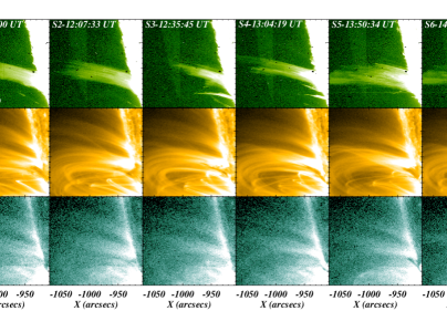
Figure 1: Homologous six surges during the peak time in IRIS 1330 Å (top-row), AIA 171 Å (middle-row), and AIA 94 Å (bottom-row). The surges are clearly visible in IRIS/1330, moderately visible in AIA 171Å, and rarely visible in AIA 94 Å.

3.1 Evolution of Surges

In this section, we describe the evolution of the first surge, using IRIS/SJI 1330 Å, AIA 304 Å, AIA 171 Å, and AIA 94Å observations. This surge was originated around 11:21 UT, however, IRIS/SJI 1330 Å observation is not aviliable at this particular time (top-row; Fig 2). The concerned surge is clearly visible in AIA 304Å, however, AIA 171 Å filter shows emissions only in and around the base of surge. Interestingly, we do see the less and faded signature of the surge in the hot-temperature filter (AIA 94 Å; top-right most panel). The site of origin of the surge is outlined by blue boxes in AIA 304Å, AIA 171Å, and AIA 94Å filters (see; top-row - Fig 2).

At T = 11:29 UT, the surge is visible in all filters and the plasma is found to have an upward flow as shown by white arrows in all the four panels (see second-row; Fig. 2). Around T = 11:39 UT, the surge attains it’s maximum phase. In the last panel (at time T = 11:54 UT), we do see the signature of falling plasma, back towards the solar surface. Here AIA 94 Å observation shows the least emission as compared to other filters of AIA. In addition, it should be noted that AIA 171 Å images clearly show the presence of closed loop structures and the surge is occuring around the one of the footpoints. Finally, we can say that this surge is showing standard plasma dynamics, i.e., first the plasma is shooting up, and then it is falling back towards the solar surface because of the solar gravity. The similar plasma dynamics is observed for other surges, kept under study, too.

Meanwhile, we see the signature of origin of next surge in the last phase of this surge which is outlined by blue boxes in all four-panels of the last row of Fig. 2. Signature of the next surge is visible even in the very hot temperature filter (AIA 94 Å; rightmost panel in last row of Fig. 2).

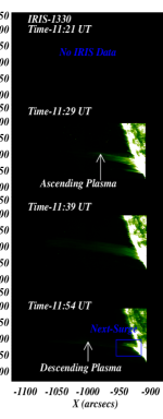
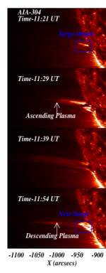
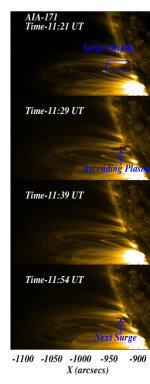
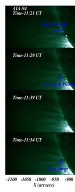
Figure 2: The evolution of the first surge (S1) in IRIS 1330 Å (first column), AIA 304 Å (second column), AIA 171 Å (third column), and AIA 94 Å (fourth column) is presented in this figure. We do see the usual behavior of the surge plasma, i.e., initially plasma flows up and later falls back onto the solar surface. The surge is clearly visible in IRIS 1330 Å and AIA 304 Å, while surge emission is comparatively less in AIA 171 Å. Further, we see few traces (especially near the base) in the hot temperature filter of AIA (i.e., 94 Å).

Next, we estimated kinematic properties of these surges e.g., life-time, velocity, acceleration, and deceleration etc. Kinematics was estimated by applying height-time (ht) technique to each surge and thus, ht profiles have been created in all the filters. These ht profiles are displayed in figure 3. Left coulmn of Fig.3 shows the reference image from IRIS/SJI 1330 Å (panel a), AIA 304 Å (panel b), AIA 171 Å (panel c), and AIA 94 Å (panel d), and slit is also plotted on each reference image (see blue-dashed lines). Note that we have used this slit to produce the ht profile for IRIS/SJI 1330 Å (panel d), AIA 171 Å (panel e), and AIA 94 Å (panel f).

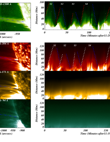
Figure 3: Figure shows the selected slit by blue dash-dotted line, which is used to produce the height-time profiles, in IRIS/SJI 1330 Å(panel a), AIA 304 Å (panel b), AIA 171 Å (panel c), and AIA 94 Å (panel d). While panel e, f, g, and h show the height-time profiles of IRIS 1330 Å, AIA 304 Å, AIA 171 Å, and AIA 94 Å, respectively. We have drawn slits during upflow (i.e., red and white dashed lines in panel e and f) and downflow phase (blue dashed lines in panel e and f), as well. These slits were utilized to estimate various properties (e.g., up flow, downflow speeds, acceleration, declaration, and life-times) of all six surges, observed in, IRIS 1330 Å (panel e) and AIA 304 Å (panel f). These properties are tabulated in table 1. We only see moderate signatures of the surges in height-time profile of AIA 171 Å and AIA 94 Å (see; panel g and h), that’s why the slits are not plotted here in.

Evolution of all the surges, under study, is clearly visible in IRIS/SJI 1330 Å and AIA 304 Å filters. The ht profiles are depicted by S1, S2 and so on. Ascending and descending phase of each surge, in thse two filters, are overplotted with the dashed lines to calculate the upflow velocity, downflow velocity, acceleration, deceleration and life time. Ascending phases in IRIS-1330 Å and AIA 304 Å are oveplotted by dashed red and white lines, respectively. Whereas, descending phases for both the filters are overplotted by dashed blue lines. On the basis of drawn path on the ht profile, S1 starts from 11:19 UT and lasts till 11:54 UT with a total life-time of $\sim$37 minutes. In S1 plasma is ascending up with a veocity of $\sim$100.0 km s^-1, alongwith the acceleration of 208.33 m s^-2 and then plasma falls back with a speed of 155.0 km s^-1 along with deceleration of 393.80 m s^-2. In the same way, we have estimated these parameter for other surges too. Parameters estimated for all the surges (from IRIS 1330 Å ht profiles) are tabulated in table 1). Additionally, we would like to emphasize that ht profiles created from AIA 171 Å and AIA 94 Å also show the signatures of surges but less prominent in comparison to the IRIS/SJI 1330 Å and AIA 304 Å.

Please note that the kinematics of surges has already studied in many of previous works. The previous findings reported that surges move upward at with the speed of 20–200 km s^-1, reach heights of up to 200,000 km, and typically last for 10–20 minutes (Roy 1973; Bruzek & Durrant 1977; Chae et al. 1999). Recently, Bong et al. (2014) have investigated 14 surges using Hinode/SOT observations, and they reported that the lifetime of the surges vary from 28.0 to 91.0 minutes, with a mean lifetime of 45.0 minutes. Further, they have reported acceleration of 100 m s^-2 and deceleration of 70 m s^-2 in surges. Kayshap et al. (2013a) have also reported that surge plasma propagates with the speed of $\sim$100 km s^-1 while the lifetime of the surge is more than 20 minutes. Findings of the present study are in accordance with that of previous studies with reference to surge kinematics.

Parameters	S1	S2	S3	S4	S5	S6
Time-Span (UT)	11:19-11:56	11:54-12:20	12:20-12:49	12:50 - 13:30	13:36-13:59	14:05-14:55
Life-time (Minutes)	$\sim$ 37.0	$\sim$26.0	$\sim$ 29.0	$\sim$40.0	$\sim$ 23.0	$\sim$ 50.0
Upflows speed (km s-1)	100.00	101.56	143.33	145.83	91.66	116.66
Acceleration (m s-1)	208.33	184.19	477.76	303.81	152.76	216.60
downflows speed (km s-1)	155.0	120.83	76.66	140.74	162.52	159.26
Deceleration (m s-1)	294.92	251.79	127.76	260.63	677.08	294.92

Table 1: Various parameters of studied surges (e.g., time, life-time, upflows, downflows, acceleration and decelration) are tabulated in this table.

3.2 Thermal Structures of Surges

We investigated the thermal nature of surges with the help of SDO/AIA observations. We have performed the DEM analysis using the sparse inversion method (Cheung et al. 2015b) for six different filters of SDO/AIA (viz. 94 Å, 131 Å, 171 Å, 193 Å, 211 Å, and 335 Å). The sparse inversion has been validated against a diverse range of thermal model, and it gives positive definite DEM solutions. In addition, the sparse diversion technique can be used in the generation of a sequence of DEM images as it is a very fast method (e.g., Cheung et al. 2015b; Jing et al. 2017). DEM solution was obtained on a pixel-by-pixel basis on a temperature bin of 0.04 (log-scale) within the range of log T/K = 5.7 to 7.78. DEM estimated,thus, for each pixel lies within our region-of-interest (ROI). Figure 4 shows EM maps from a sparse inversion of AIA observations of NOAA AR 12114 along with S1 during its maximum phase. EM (i.e., total DEM emission for particular temperature interval) is shown in the different temperature bins. For instance, the top-left panel shows EM in the temperature regime of log T/K = [5.7 - 6.0]. Here, a little emission can be seen near the base of the surge. While the top middle-panel shows the EM for a temperature range log T/K = [6.0 - 6.3]. The surge is clearly visible within this temperature bin, as outlined by a blue rectangular box (see; top-middle panel). Spire of the surge has major emission in this particular temperature bin. Although the base of surge also emits significantly, but it was little in comparison to emission from spire region. In the next temperature bin (i.e, log T/K = [6.3 - 6.6]), we do not see much emission from the surge. Moderate emission is visible near the base of the surge in a small area in this temperature bin (see; the top-right panel of Fig. 4). However, a major emission around the base of the surge is visible in the temperature bin of log T/K = [6.6 - 6.9] (see bottom left-panel of Fig. 4). We also see little emission near the base of the surge in the temperature bin of log T/K = [6.9 - 7.2]. While investigating other surges (i.e., from S2 to S6) using the similar approach we found similar behavior (plots not shown here).

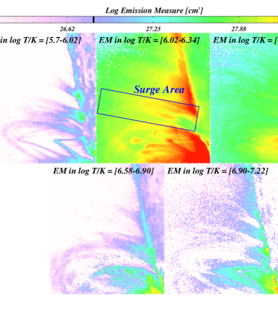
Figure 4: In this figure, we present the EM maps in various temperature ranges (temperature range is written on each EM map) for S1. The blue rectangular box in the top-middle panel outlines the surge area, and a significant surge’s emission does exist in this temperature range (i.e; log T/K = 6.0 - 6.3). We do see a relatively small emission near the base in the next temperature bin (i.e., right-top panel; log T/K = 6.3-6.6). Interestingly, in temperature bin of log T/K = 6.6-6.9, a significant emission especially near the base justifies the heated base. Again, the next higher temperature bin (i.e., log T/k = 6.9-7.2) is showing very little emission near the base.

Further, we investigated the DEM distribution from two different regions (i.e., base and spire region) of all the surges under study. The top-left column of figure 5 displays the DEM from base (black histogram) and spire (blue histogram) of S1. In this figure, two peaks for base region at log T/K = 6.37 and log T/K = 6.93 are clearly visible. This DEM data is fitted with double Gaussian (see; overplotted black solid line – top-left panel of Fig. 5), justifying the presence of two separate distributions. Peaks of these two Gaussians are shown by vertical black-(cool component) and green-(hot component) dashed lines. It should be noted that the cool component (i.e., around log T/K = 6.37) has a higher DEM compared to the DEM of hot peak. And, the spread (i.e., Gaussian sigma) of the hot component DEM distribution is almost double (0.341) of that for the cool component DEM distribution (0.189). As the DEM of spire shows only a single peak, it was fitted with a single Gaussian (see overplotted solid blue line). The dashed blue vertical line shows the peak of DEM (at log T/K = 6.34). Thus, we can say that hot component does not occur within the spire plasma of S1. In addition, the spread of DEM distribuation of the cool component is found narrower for spire (0.11) as compared to that of base (0.189). Similar analysis have been performed for other surges as well (S2: top-middle panel, S3: top-right panel, S4: bottom-left panel, S5: bottom-middle panel, and S6: bottom-right panel) and it is observed that all the surges show similar behavior. Parameters obtained from the Gaussian fitting of DEM distributions are tabulated in table 2 for base and in table 3 for spire, respectively. Tabulated parameters suggest that: (a) there is comparatively higher cool emission at the base of surges, although, the hot emission is also significant at the base of each surge. (b) peak position for cool component is around log T/K = 6.35 and that of hot component is around log T/K = 6.95 (c) spread of the hot component is double as that of cool component, and (d) spread of the DEM distribution for cool component is narrow for spire region.

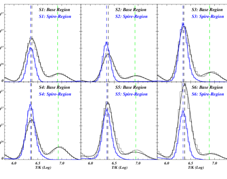
Figure 5: The figure shows the distribuation of DEM from the base (black histogram) and spire (blue histogram) for all six surges. Displayed DEM maps are obtained from the maximum phase of the corresponding surge. DEM distribution of base region shows two peaks. While, DEM distribition of spire has only one peak. Hence, we have fitted the base DEM with double Gaussian function (black curve) and spire DEM with a single Gaussian functions (blue curve).

Surge id (Base)	DEM Peak value[1/2] (cm${}^{-5})$)	Centroid temperature[1/2] (log T/K)	Gaussian Sigma[1/2] (logT)
S1	1.4$\times$1027/4.4$\times$1026	6.37/6.91	0.186/0.341
S2	8.8$\times$1026/2.8$\times$1026	6.37/6.93	0.177/0.344
S3	1.78$\times$1027/5.57$\times$1026	6.35/6.89	0.171/0.371
S4	1.34$\times$1027/5.92$\times$1026	6.36/6.62	0.184/0.311
S5	1.62$\times$1027/2.03$\times$1026	6.36/6.95	0.152/0.305
S6	2.29$\times$1027/3.44$\times$1026	6.37/6.88	0.166/0.377

Table 2: We fitted the double Gaussian function on the base DEM of each surge. The Gaussian fitting gives the peak values of DEM, centroid temperature, and Gaussian width (spread of the distribution) of cool component and hot component. We tabulated all three parameters for the cool component (with suffix 1) as well as the hot component (with suffix 2) in this table. "1/2" referes to "cool component/hot component".

Surge id (spire)	DEM Peak value(cm${}^{-5})$)	Centroid temperature (log T/K)	Gaussian Sigma (log T/K)
S1	1.0$\times$1027	6.34	0.11
S2	1.10$\times$1027	6.34	0.11
S3	1.71$\times$1026	6.33	0.117
S4	1.61$\times$1027	6.34	0.121
S5	1.45$\times$1027	6.36	0.152
S6	1.41$\times$1027	6.34	0.115

Table 3: Same as table 2 but for the spire of surges. It should be noted that spire of surges has only one peak unlike the DEM of base of the surges.

3.3 Spectoscopic Evolution of Surges

IRIS provides high-resolution spectral observations of these six homologous surges. IRIS slit has been placed in the spire region (i.e., far away from surge’s bases; see white-dashed line in left-panel of Fig. 6) of all the surges. Unfortunately, we do not have the spectroscopic observations near the base of these surges. However, the available IRIS spectroscopic observations (i.e, spectra far-away from the bases of surges) still provides important information about these surges.

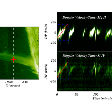
Figure 6: Left-panel shows the IRIS/SJI 1330 Å image of the surge along with the slit position (white-dashed line). The right-panel shows Doppler velocity-time diagram for Mg ii k (top-panel) and Si iv 1402.77 Å (bottom-panel) that is taken from one particular y-position (i.e., y = -208.56 arcsec) shown by a plus red symbol in the left-panel. The wavelength is transformed into Doppler velocity using standard rest wavelengths taken from CHIANTI atomic database, i.e., 1402.77 Å and 2796.35 Å for Si iv and Mg ii k, respectively. Please note that both spectral lines have significant emission during these surges as the counts are significantly high. First surge is outlined by the blue rectangular box in both panels. Initially, both lines are blueshifted that shifts towards the red-shifts with time. The transformation from blue- to red-shifts is very gentle as outlined by solid red lines in both panels.

We utilized few important IRIS lines, viz. Mg ii k 2796.35 Å, Mg ii h 2803.52 Å, Si iv 1402.77 Å, and O iv 1401.15 Å, for the analysis of these surges. Left-panel of figure 6 displays the IRIS/SJI 1330 Å image along with slit-position shown by white-dashed line, i.e., the location within which IRIS has captured the surge spectra. Further, the Doppler velocity-time (v-t) diagram for prominent Mg ii 2796.35 Å (top-right panel) and Si iv 1402.77 Å (bottom-right panel) emissions are also displayed in the figure 6. The wavelength is converted into Doppler velocity using the standard wavelength of these lines as provided by CHIANTI atomic database, namely, 2796.35 Å for Mg ii k and 1402.77 Å for Si iv line. Signal-to-noise (SNR) ratio is very high during the surges, and the rest of the slit area is having almost no signals. All the surges are very clear in the v-t diagram of Mg ii 2796.35 Å and Si iv 1402.77 Å lines, i.e., bright areas in both right-panels of figure 6.

Further, the v-t diagram also reveals that both the lines (i.e., Mg ii and Si iv) are highly blueshifted at the time of origin. The blueshift decreases with time and inverts into redshift. Solid red lines on both v-t diagrams (i.e., S1; both right-panels; figure 6) exhibit the linear transition for the doppler velocity. This transition was observed for the other sugers too. In addition, the maximum blue- and red-shift is observed in the strongest surge (i.e. S6) which starts almost after 160.0 minutes from the start of first surge.

Both the lines were fitted with a single Gaussian to produce the Intensity, Doppler Velocity and Sigma Maps for complete observation which are shown in the appendix Diagnostic of Homologous Solar Surge Plasma as observed by IRIS and SDO (see, figure 10 for Mg ii k 2796.35 Å and figure 11 for Si iv 1402.77 Å lines).

With the careful inspection of these spectroscopic parameter maps, following can be concluded about the general behavior of these surges: (1) blueshift dominates the first half lifetime of the surge, while redshift is dominent in the second half lifetime, (2) Gaussian sigma is higher for blueshift regions (i.e., first half lifetime of surges), and (3) Si iv line maps are fuzzier compared to Mg ii 2796.35 Å.

3.3.1 Evolution of Si iv

We have studied the evolution of Si iv 1402.77 Å during the most dynamic surge (i.e., last surge: S6). IRIS/SJI 1330 Å image of surge is displayed in the panel A of figure 7. Blue-dashed rectangular box, along with a vertical solid blue line, outlines the core material of surge. The intensity-time map of Si iv for S6 is presented in panel B of figure 7. A blue vertical line in the vicinity of surge’s core plasma is drawn on the Si iv intensity-time map (cf., panel B of figure 7). This location has been used to study the evolution of Si iv spectral line. More precisely, thick horizontal dashes are displayed by different colors within the surge’s core material (i.e., blue-dashed box in panel A) corresponding to the spectral profiles that are shown in the right column of figure 7 (i.e., panels C1 to C5). It must be noted that these locations cover the full vertical extent of this surge.

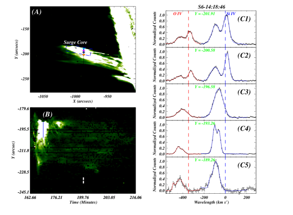
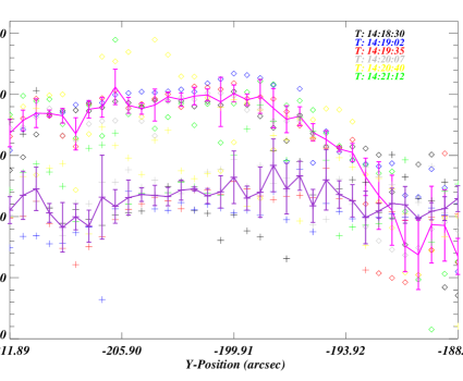
Figure 7: Panel A displays IRIS/SJI 1330 Å along with a blue-dashed rectangular box that outlines the surge’s core plasma. The panel B shows Si iv intensity-time diagram of S6. To show the spectral profiles, we selected five different locations shown by horizontal slits of different colors in panel A, namely, C1-red, C2-yellow, C3-black, C4-magenta, and C5-cyan. The panel C1 clearly shows the double peak in Si iv and O iv spectral profiles at the lower edge of S6 (i.e., Y = -201.99$"$). Therefore, they are fitted with double Gaussian function (i.e., solid blue-line for Si iv and red-line for O iv). At the next position in S6 (i.e., Y = -200.58$"$), we found the similar profiles (see; panel C2) while almost single Gaussian profiles exist for both lines at Y = -196.58$"$ (see; panel C3). Further, at the next y-position = -193.26$"$ the double peak exists again in both lines, however, both peaks are completely shifted into blue-regime. Finally, the similar behavior of both lines is present at the other (upper) edge of S6 (panel C5). In the bottom panel, we have shown the variations of Doppler velocities for both components of Si iv (i.e., both peaks) from six different times as mentioned in the bottom-panel. The Doppler velocity of varying (non-constant) peak is shown by the diamond of different colors as per time while the Doppler velocity of constant peak by plus signs of different colors as per the time. Finally, we averaged all time points at each y-position for both peak and shown the averaged Doppler velocity by solid pink line (one peak) and purple line (another peak). We see that one peak (solid pink line) shifts from red to blueshift as we move from one edge to another edge of S6, i.e., varying or non-constant component while another peak (solid purple line) shows almost constant Doppler velocity, i.e., constant component.

Panel C1 shows the Si iv and O iv spectral profiles from the bottom-end of surge’s core plasma (i.e., red dash in blue-box; panel A). Si iv line shows two components, one on red-side and another on blue-side. Similar behavior is observed for O iv line, as well. Si iv and O iv lines were fitted with two Gaussians. Fitted curves are overplotted on the observed spectra by blue color for Si iv and red color for O iv spectral lines, respectively. Observed profiles are very well characterized using this double-Gaussian approach. Blue- and red-dashed vertical lines lie at the zero velocity for Si iv and O iv, respectively.

Next-panel (C2), shows the profile from a location shown by yellow dash in the blue-rectangular box (see; panel A). Here, line profile exhibits a similar behaviour as that in C1. Panel C3 shows the profile obtained from near the middle of the core plasma (i.e., black dash in panel A). For both the lines, obtained profiles are having almost a single peak. Thus, these profiles were fitted using a single Gaussian function. Further, as we move towards the upper edge of surge plasma, double peak profile starts appearing again for both the lines (see; panel C4–profile from the location shown by magenta dash in panel A and panel C5–profile from upper edge of surge plasma and it is shown by cyan dash in panel A). However, new peaks (or components) are blue-shifted for both lines. Interestingly, One component (or peak) of Si iv is always constant at -100 km/s at this particular instant of time (shown in panels from C1 to C5) that is defined as the constant velocity component. On the contrary, other component (or peak) of Si iv changes from red-side (near the bottom edge) to blue-side (near the top-edge) along with the absence of this particular component (i.e., single Gaussian– constant component at -100 km/s) around the middle of S6. This secondary component, which changes from redshifts (at bottom edge) to blueshifts (at upper edge), is defined as the varying (or non-constant velocity) component. This finding refers to the observation at a single instant of time (i.e. 14:18:46), for different positions across the surge.

We have chosen six different times that are mentioned in the bottom panel of Fig. 7. We estimated the Doppler velocities of constant and varying (non-constant) components (as defined above) for all the Y-positions across S6 at the mentioned six different times. Deduced Doppler velocities, as a function of Y-position (i.e., positions across S6), are shown in the bottom panel of Fig. 7. Doppler velocites of constant and non-constant components are shown by plus and diamond symbols, respectively. Next, we averaged all the Doppler velocites at a given Y-position (for all the considered time instants) for both the constant and non-constant components, separately. Averaged Doppler velocity profiles are overplotted by solid pink and purple lines for constant and non-constant components, respectively. Here, error bars refer to the standard deviations at each Y-position. From this analysis, it can be concluded that Si iv spectral line has constant (i.e., having Doppler velocities around -100 km s^-1 at all y positions during the selected times), and non-constant component. Doppler velocity of this non-constant component changes from low red-shifts of $\sim$20 km s^-1 (at the bottom edge of S6) to very high blue shifts of $\sim$-140.0 km s^-1 (at the top edge of S6). We performed the similar analysis for other surges too (i.e., for S1 to S5) and a similar behaviour of Si iv spectral line profiles for rest of the surges is found (see appendix B).

3.3.2 Opacity $\&$ Evolution of Mg ii resonance lines in the homologous surges

Mg ii k $\&$ h lines are transitions to a common lower level from finely splitted upper levels (Leenaarts et al. 2013; Kerr et al. 2015). Intensity ratio of Mg ii k $\&$ h (i.e., R_kh) lines can be used to investigate the opacity (e.g., Schmelz et al. 1997; Mathioudakis et al. 1999). The transitions of Mg ii resonance lines involve the same element (Mg) in the same ionization state. The escape probability of a photon is unity for optically thin conditions. Hence, in optically thin conditions, intensity ratio of the Mg ii k 2796.35 Å to Mg ii h 2803.52 Å is simply the ratio of the oscillator strengths, i.e., R_kh should be equal or greater than two (Kerr et al. 2015). While, in case of optically thick atmosphere, this ratio is smaller (Kerr et al. 2015).

 

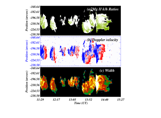
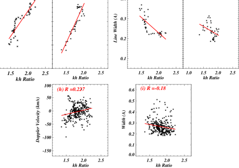
Figure 8: In this figure, we have shown three maps, namely, Mg ii k/h ratio map (R_kh; panel a), Doppler velocity map (panel b), and width map (panel c). Further, we have shown the correlations, namely, (1) correlation between Doppler velocity and R_kh for S1 (panel d) and S2 (panel e) and (2) correlation between Gaussian width and R_kh for S1 (panel f) and S2 (panel g). We found the tight and positive correlation between Doppler velocity and R_kh for S1 (Pearson coefficient = 0.877) and S2 ((Pearson coefficient = 0.886). While we found a negative correlation between Gaussian width and R_kh for S1 (Pearson coefficient = -0.77) and a weak negative correlation between Gaussian width and R_kh for S2 (Pearson coefficient = -0.38). We collected these three parameters (i.e., R_kh, Doppler velocity, and Gaussian width) from all surge and then, we averaged them for all the surges. Finally, we displayed both the correlations from these averaged parameters (see panel h: correlation between Doppler velocity and R_kh and panel i: correlation between Gaussian width and R_kh). Overall, we find weak positive correlations between Doppler velocity and R_kh (panel h) and a weak negative correlation between Gaussian width and R_kh (panel i).

We have estimated R_kh for the complete observation. And, R_kh map along with Doppler velocity and Gaussian sigma maps are shown in panel a, b, and c of Fig. 8, respectively. First, we investigated the correlation among R_kh, Doppler velocity, and Gaussian sigma for S1. R_kh is found to be low (i.e, 1.4) for the initial phase of S1 and it increases as time progresses. Blueshift in S1 decreases with the time and inverts into redshifts around the midtime for S1. This redehift further increases with time. Interestingly, R_kh is positivley correlated with the Doppler velocity pattern (i.e., blueshifts decrease with time, and finally inverts into redshifts followed by the increase in Doppler velocity.) Gaussian width is, however, negativley correlated with R_kh, i.e., R_kh increases with decreasing Gaussian width. Panels (d) and (e) of Fig. 8 show the correlation between R_kh and Doppler velocity for S1 and S2, respectively. From the figures it is evident that R_kh and Doppler velocity are tightly $\&$ positively correlated, as Pearson’s coefficents for S1 and S2 are 0.887 and 0.886, respectively. Correlation between R_kh and Gaussian width for S1 and S2 are shown in panel (f) and (g) of Fig. 8, respectively. These two parameters are negatively correlated and Pearson’s coefficent for S1 and S2 are -0.77 and -0.38, respectively.

For the final correlation plots, parameters (i.e., R_kh, Doppler velocity, and Gaussian width) were averaged over all the y-positions at each instant of time of all six surges. Hence, we got averaged array of each parameter that includes all surges. Finally, panel (g) and panel (i) of Fig. 8 shows the correlation between R_kh $\&$ Doppler velocity, and R_kh and Gaussian width, respectively, averaged over all the surges. Correlation between R_kh and Doppler velocity, averaged over all the surges, is positive and has the Pearson’s coefficent value of 0.227. Correlation between R_kh and Gaussian width, averaged over all the surges, is negative and has the Pearson’s coefficent value of -0.18.

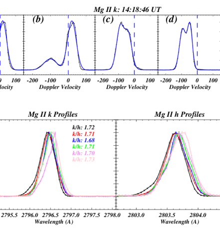
Figure 9: Top-row shows Mg ii k line taken from five different y-positions (i.e., same locations as displayed by horizontal slits by various colors in the panel A of figure 7) during the evolution of S6 at T = 14:18:46 UT. We see a double peak profile for Mg ii k line. One peak is constant while the other is shifting from red-shift at one edge of S6 (first-panel) to blue-shift at another edge of S6 (last-panel). This component is varying or non-constant component as defined already. In the bottom row, we have shown some Mg ii k (bottom-left panel) and Mg ii h (bottom-right panel) with different colors from the later phase of S6. In addition, we have mentioned also the R_kh values for these spectral profiles. It is clearly visible that Mg ii k $\&$ h profiles are a single peak during the optically thick conditions.

Mg ii k 2796.35 Å line generally gets observed in the optically thick condition. Therefore, the complex behavior of Mg ii k line (i.e, double, triple, or multi-peak profile) do exist in the solar atmosphere. Although, in many circumstances Mg ii lines are single peak profiles, for instance, sunspot umbrae (Tian et al. 2014), solar flares (Kerr et al. 2015), and filaments (Harra et al. 2014). In addition, outside of the limb, Mg ii k lines exhibit single-peak profile (Tei et al. 2020). Therefore, in present scenario as spectra was taken far away from the limb (see IRIS slit in the left-panel of figure 6 – white dashed line), we believe that Mg ii lines should be single peaked profiles. Data obtained for Mg ii k 2796.35 Å in S6 exhibit two peaks (see; top-panel of figure 9). It can be noted that the double peak profile exists only in the initial phase of surges, which becomes single peak profile in the later phases of surges. We have already established the rotating motion for all the surges (see; figure 7 $\&$ 12) in TR. Rotating motion leads to the double peak in Si iv and O iv emission (i.e., optically thin lines). In principle, we should also see the rotating motion in chromospheric plasma,i.e., emission captured by Mg ii k $\&$ h lines. Mg ii k 2796.35 Å profiles across S6 from time 14:18:46 UT are displayed in the top-panel of figure 9. At the bottom-edge of S6, we observe peaks in the blue- and red-regimes of Mg ii k 2796.35 Å line (panel a). Similar Mg ii 2796.35 Å profile exists in another location a little far away from the bottom-edge (panel b). However, in panel c, both peaks in Mg ii line have shifted to the blue-regime. Further, last two panels (i.e., panel d and e) also exhibit similar behaviour. The profiles of panel d and e are taken from near the upper edge of S6. Both the peaks of Mg ii line, at the upper edge of S6, lie in the blue-regime. Here also, the postion of one peak (in blue-regime) is constant (i.e., constant component) while other peak changes from redshifts at the lower edge of S6 to blueshifts at the upper edge of S6 (i.e., varying or non-constant component). This behavior is similar to that of Si iv and O iv (see subsection 3.3.1) emissions. Thus, it can be concluded that double peak Mg ii profiles also aries due to simultaneous presence of rotational and translational motions in the surge plasma.

Rotating motion of the surge plasma column is not a stable feature. It decays with time and vanishes after some time in each surge, e.g, after $\sim$15.0 minutes from the origin for S6. Thus we only see single peaks in Mg ii k $\&$ h profiles in the later phase of the surges (as shown for S6 in the bottom row of the figure 9). Please note that even for the single peak profiles, Mg ii k $\&$ h lines are still getting formed in optically thick-regime (i.e., R_kh values are around $\sim$ 1.72 for the profiles displayed in bottom-panel of figure 9).

4 Discussion and Conclusions

We utilized high-resolution SDO/AIA and IRIS observations to study six homologous surges that originated from AR 12114, located at the limb. These six homologous surges were originated within the time-span of $\sim$ 4 hours on 7^th July 2014 from AR 12114. In the present study we started with the estimation of the kinematics of all surges using IRIS and SDO/AIA imaging observations. Variations in the lifetimes, up-flow and down-flow speeds, acceleration, and deceleration were found for these surges. Lifetime of surges varies from 23.0 to 50.0 minutes. Up-flow speed varies from 91.66 km s^-1 to 145.83 km s^-1. Acceleration varies from 152.97 m s^-2 to 477.27 m s^-2. Down-flow speed varies from 76.67 km s^-1 to 165.52 km s^-1. Deceleration varies from 127.76 ms^-2 to 667.08 m s^-2. Thus, it can be said that these homologous surges exhibit a large variation in kinematics.

DEM of the surge’s base shows the presence of two different temperature peaks, i.e., cool temperature distribution – log T/K = 6.0 - 6.3, and hot temperature distribution – log T/K = 6.6 - 7.0. While, the spire (a region very far away from the base) of all surges emits only in the cool temperature regime (i.e., log T/K = 6.0 - 6.3 K). Thus, DEM analysis provides an important finding that there is existance of heated plasma at the origin site of the surges.

The most striking feature of the present observation baseline is finding the emission of the surges in Si iv, O iv, and Mg ii k $\&$ h lines. Majority of the previous works have reported the surge emission in H_α or Ca ii 8542 Å (e.g., Schmieder et al. 1995; Canfield et al. 1996; Kim et al. 2015; Huang et al. 2017; Yang et al. 2019). Recently, Nóbrega-Siverio et al. (2017) have reported the emission of surge in Si iv only with the help of IRIS observations. However, the present observations provide a broader range of surge’s emission, i.e., emission of surges in Mg ii k $\&$ h, Si iv and O iv lines. Here we report the surge’s emission in two TR lines (i.e., Si iv, and O iv) and chromospheric Mg ii resonance lines (i.e., k $\&$ h). Thus, this is the first report on the surge’s emission in Mg ii resonance lines and O iv, and second work that report surge’s emission in Si iv after Nóbrega-Siverio et al. (2017).

Shape of the spectral profiles is crucial as it provides important information about operating/on-going dynamics and physical process(es) within the in-situ plasma, e.g., bi-directional flows lead two distinct satellite lines during the explosive events (Dere et al. (1989)), enhanced wing emission in TR spectral lines above the networks that leads asymmetries in spectral profiles (Peter 2000), several mechanisms may introduce the asymmetry in the coronal extreme ultraviolet lines originated within the active-regions (Peter 2010), broadening of profiles due to hot explosion (Peter et al. 2014), and asymmetric profiles because of the prevalence of twist in the chromosphere/TR (De Pontieu et al. 2014). Peter (2000) and Peter (2010) have demonstrated that double-Gaussian yields a reliable fitting for TR/coronal spectral profiles.

IRIS provides the time-series spectral observations from the spire of surges under consideration. The v-t diagrams exhibit a systematic shift of Mg ii and Si iv lines from blue-shifts to red-shifts within the life-time of surges. The blueshifts means that the plasma is flowing upward, while redshift means plasma falling back towards the solar surface. The height-time diagrams (produced using imaging observations) also show that plasma is propagating in the upward direction in the first half of life-time while plasma is falling back towards the solar surface in the latter half of life-time of each surge. We do see the up-flow and downflow episodes of surges from the height-time diagram produced using imaging observations from IRIS and AIA. The similar dynamics of surges can also be inferred from the v-t diagrams of Mg ii and Si iv lines.

Further, it is observed that the spectra of all lines for initial phase of each surge exhibits two peaks. Here, one of the component is constant (i.e., spectral line center does not change across the surges, for example, it is $\sim$ -100 km s^-1 in case of S6), while other component is varying (non-constant) across the surges (i.e., moves from the red-shifts to blue-shifts as we move from one edge of the surge to another edge). This is true for both, optically thin (i.e, Si iv and O iv) and optically thick (i.e., Mg ii k) lines. The constant component occurs due to the translational motion while the varying or non-constant is a result of rotational plasma. This the varying component changes from redshifts to blueshifts as we move from one edge of the surge to another edge, which is a typical signature of the rotating plasma. Rotating plasma has also been reported in other jet-like structures of solar origin (e.g., Pike & Mason 1998, and refernces cited therein; Curdt & Tian 2011, and refernces cited therein; De Pontieu et al. 2014, and refernces cited therein; Young & Muglach 2014, and refernces cited therein; Cheung et al. 2015a, and refernces cited therein; Kayshap et al. 2018a, and refernces cited therein).

Magnetic reconnection process, that converts magnetic energy into thermal energy, may happen due to several activieits, e.g., flux-emergence, moving magnetic features, convective motions, etc. These processes are the fundamental base for majority of numerical simulations exhibiting the formation of jet-like structures within the solar atmosphere (e.g., Yokoyama & Shibata 1995, 1996; Nishizuka et al. 2008; Pariat et al. 2010; Srivastava & Murawski 2011b; Kayshap et al. 2013b; Jelínek et al. 2015; Wyper et al. 2017). More specifically, numerical simulations based on the magnetic reconnection between the twisted and pre-existing simpler magnetic field leads to the helical or twisted field lines. Flow of plasma through these helical/twisted magnetic field lines appears as the rotating motion of the jet-plasma column (Pariat et al. 2009, and references cited therein; Pariat et al. 2016, and references cited therein; Fang et al. 2014, and references cited therein; Cheung et al. 2015b, and references cited therein). And, energy produced in the magnetic reconnection process heats the plasma, that appears as the brightened/heated base for these jet-like structures in the observations (e.g., Shibata et al. 1992; Yokoyama & Shibata 1995; Uddin et al. 2012; Kayshap et al. 2013a, b, 2018b). We have already established that the bases of the observed surges are heated, i.e., hot temperature component (Log T/K = 6.6-7.0) exists in the DEM of surge’s base (figure 5). Thus, our analysis (e.g., heated plasma at the base of surges and rotating/helical motion) indicates the occurrence of the magnetic reconnection in the support of the formation of homologous surges as reported previously in various works (e.g., Schmieder et al. 1995, and references cited therein; Brooks et al. 2007, and references cited therein; Uddin et al. 2012, and references cited therein; Kayshap et al. 2013a, and references cited therein). The amount of the released energy can vary from case to case, as the magnetic field and plasma conditions may vary spatially and temporally. Therefore, variations in the released energy during these homologous surges can be expected which leads to a large variation in the kinematic parameters (e.g., life-time, up-flow/down-flow, and velocity) of these surges.

Usually, double (or multi) peak exist in the Mg ii k 2796.35 Å profiles for quiet-Sun and coronal holes (Peter et al. 2014; Kayshap et al. 2018b). However, Mg ii profiles are observed without the central reversal feature (i.e., single peak) in the flaring region, yet the line is optically thick (Kerr et al. 2015). Sunspot umbrae also show the single peak profiles despite the optically thick nature of Mg ii lines (Morrill et al. 2001). The current umbral models, assuming optically thick conditions, can not produce the single peak Mg ii k 2796.35 Å profiles. Usually, decoupling between source function and Planck function in mid-chromosphere leads to the formation of central reversal or double peak profiles (Leenaarts et al. 2013). However, for high-density plasma, coupling between line source and Planck function can continue even after the mid chromosphere. Thus, in such scenarios single profiles are observed (Kerr et al. 2015).

Generally outside the limb, Mg ii profiles exhibit a single peak (e.g., Feldman & Doschek 1977; Vial et al. 1981; Harra et al. 2014). Furthermore, spectral lines become narrower as we move away from the limb. However, in our case, we see both the double (initial phase) as well as a single peak (in the later phases of surges) profiles for surges. Here, double-peak profiles arise due to simultaneous presence of rotational and translational motion in the surges plasma, and not because of an optically thick atmosphere. In the later phase of surges (as rotation vanishes with time), for optically thick Mg ii, single peak Mg ii k $\&$ h profiles are observed. Optically thick conditions were revealed by R_kh (i.e., R_kh < 2.0). Please note that R_kh has been measured for different plasma conditions, e.g., R_kh = 1.14-1.46 in various features (Kohl & Parkinson 1976; Lemaire et al. 1981, 1984), R_kh = 1.20$\pm$0.010 in the non-flaring regions (Kerr et al. 2015), R_kh = 1.07–1.19 in the region surrounding the flare emissions (before, during, and after the flare; Kerr et al. 2015), and R_kh = 1.40–1.70 in the filament material (Harra et al. 2014). In present work, averaged R_kh varies from 1.40 to 2.20 in the surges (see; figure 8). On an average, R_kh value for surges seem to be higher as compared to that for other features. We have investigated the correlation of R_kh with the Doppler velocity and width (see; Fig. 8), also. R_kh value increases with Doppler velocity pattern of surges, i.e., the blueshifts decrease with time, and inverts into the redshifts, followed by a increase in redshifts. R_kh is positively correlated with the above described Doppler velocity pattern of surges, while R_kh is negatively correlated with Gaussian width, i.e., R_kh increases as Gaussian width decreases. It should be noted that Doppler velocity follows the above-described pattern and Gaussian width decreases as time progress for each surge. Hence, we conclude that R_kh increases with the time as each surge progresses. It is to mention that Harra et al. (2014) have also reported an increase in the R_kh following a filament eruption, for off-limb observations.

Generally, a higher intensity line is an indicative of a density enhancement which can directly affect the shape of the line as mentioned by Kerr et al. (2015). However, in case of optically thick lines, other mechanisms (e.g., radiation) can also populate the upper levels of resonance line. Harra et al. (2014) reported that R_kh would be closer to 4 if radiation is an important process in the particular in-situ plasma. Hence, the absorption of radiation in the present scenario can be ruled out as we did not find such intensity ratios. Recent modeling, using bifrost (Gudiksen et al. 2011) and the radiative transfer (Pereira & Uitenbroek 2015) codes, predicts that if there is a large temperature gradient ($\geq$1500 k) between the temperature minimum and formation region, Mg ii lines can undergo emission only (Pereira et al. 2015). In case of the flaring region, Kerr et al. (2015) reported the formation of single peak Mg ii profiles. However, it should be noted that Harra et al. (2014) has also found the single peak Mg ii profiles in cool filament above the limb. Further, the increment in R_kh values occur after the plasma eruption (i.e., filament eruption/coronal mass ejection). Surges are also plasma ejection higher up in the atmosphere from the origin site. Thus, we believe that increase in R_kh values with time is a result of plasma ejection, that in turn might be the result of some additional radiative excitation along with the collisional excitation as reported by Harra et al. (2014). Finally, we mention that numerical modeling is needed to clarify this conclusion as also suggested by Harra et al. (2014).

In conclusion, after the rigorous investigation of the kinematic properties and thermal structure of six homologous surges, with the help of IRIS, and SDO observations, we have reported, for the first time, the emission of homologous surges in various spectral lines of the interface-region. It is found that all six homologous surges exhibit the rotating motion. Collectively, heated bases of the surge and rotating motion justify the occurrence of magnetic reconnection in support of the formation of surges. In the present work we have reported the time evolution of R_kh, in case of surges, for the first time.

Data Availability

The data underlying this article are available at https://iris.lmsal.com/data.html (NASA/IRIS website) and at https://iris.lmsal.com/search/ (LMSAL search website). Note that IRIS, as well as SDO/AIA data, are publically available with the observation id OBS 3864611254.

Appendix A Intensity, Doppler velocity and width maps: Mg ii k 2796.35 Å and Si iv 1402.77 Å

Intensity, Doppler velocity, and Gaussian width maps for Mg ii k 2796.35 Å (fig. 10) and Si iv 1402.77 Å (fig. 11) are shown in this appendix. Doppler velocity and Gaussian sigma maps for Mg ii k 2796.35 Å and Si iv 1402.77 Å were produced using the complete observations. Obtained spectra (for both Mg ii k 2796.35 Å and Si iv 1402.77 Å) were first fitted with single Gaussian function. Next, the Intensity, Doppler velocity, and Gaussian sigma of the complete observations were deduced using the single Gaussian fit. Single Gaussian fit was also used to produced these spectroscopic parameter maps for both lines. Doppler velocity maps show that almost the first half of each surge is dominated by blueshifts, while the later half is redshifted, i.e., firstly the plasma is flowing up while after attaining the maximum height the plasma falls back to the solar surface. Such plasma dynamics (i.e., plasma up flow and downfall with time) is true for both Mg ii k and Si iv lines (see; middle-panels in fig. 10 and  11). Further, Gaussian width is higher in the initial phase of surges, it decrease with increasing time for both the lines Mg ii k and Si iv lines (see; lower-panels in fig. 10 and  11)line. Thus, it can be said that the dynamics of surges is similar in both chromosphere (i.e., mg ii k 2796.35 Å) and TR (i.e., Si iv 1402.77 Å).

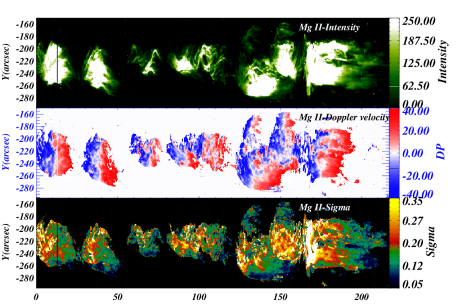
Figure 10: Intensity, Doppler Velocity and Gaussian Sigma maps for the complete observation of Mg ii k 2796.35 Å. Displayed color bars in each panel show the range of corresponding parameter.

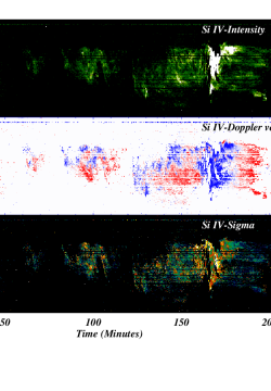
Figure 11: same as figure 10 but for Si iv 1402.77 å.

Appendix B Constant and varying (non-constant) components of Si iv: from first surge (S1) to fifth surge (S5)

In case of most prominent surge (i.e., S6), we have already presented the dynamics of constant and varying or non-constant components in both the lines (see; section 3.3.1 and  3.3.2). We have also investigated the dynamics of constant and varying or non-constant components for the rest of the surges, i.e., from S1 to S5. Behavior of both components were investigated by taking average of spectra over time-span of the surge emission. Averaged spectra were fitted using a double Gaussian function. Doppler velocity of both the components at each y-position was estimated on the basis of double Gaussian fitting. We utilize the same procedure to deduce the Doppler velocity of constant and varying components for all other surges.

Figure 12: Here we show the behavior of primary and secondary components of Si iv line for S1 (top-left panel), S2 (top-right panel), S3 (middle-left panel), S4 (middle-right panel), and S5(bottom panel). The primary component shows constant values across all y-position in all surges, i.e., it is a constant component. While the secondary component shifts from red-shift to blueshift in all surges, i.e., it is a varying component.

At last, we have shown the Doppler velocity variations of constant and varying components for S1 (top-left panel), S2 (top-right panel), S3 (middle-left, panel), S4 (middle-right panel), and S5 (bottom-panel) in figure 12. In case of S1 (top-left panel), we do see that varying component is changing from redshift of $\sim$ 50 km s^-1 to blueshift of -100.0 km s^-1. While the constant component lies at $\sim$ -40.0 km s^-1 in all y-positions across the S1. Please note that similar type of results were found for other surges too (see other panels in fig. 12). Thus, it can be concluded that for all the surges, one component shifts from the redshift to blueshift (i.e., varying component), while other component has constant velocity (i.e., non-constant).

References

- Asai et al. (2001) Asai A., Ishii T. T., Kurokawa H., 2001, ApJ, 555, L65
- Bohlin et al. (1975) Bohlin J. D., Vogel S. N., Purcell J. D., Sheeley N. R. J., Tousey R., Vanhoosier M. E., 1975, ApJ, 197, L133
- Bong et al. (2014) Bong S.-C., Cho K.-S., Yurchyshyn V., 2014, Journal of Korean Astronomical Society, 47, 311
- Brooks et al. (2007) Brooks D. H., Kurokawa H., Berger T. E., 2007, ApJ, 656, 1197
- Bruzek & Durrant (1977) Bruzek A., Durrant C. J., 1977, Illustrated glossary for solar and solar terrestrial physics, doi:10.1007/978-94-010-1245-4.
- Canfield et al. (1996) Canfield R. C., Reardon K. P., Leka K. D., Shibata K., Yokoyama T., Shimojo M., 1996, ApJ, 464, 1016
- Chae et al. (1999) Chae J., Qiu J., Wang H., Goode P. R., 1999, ApJ, 513, L75
- Chen et al. (2008) Chen H. D., Jiang Y. C., Ma S. L., 2008, A&A, 478, 907
- Cheung et al. (2015a) Cheung M. C. M., et al., 2015a, ApJ, 801, 83
- Cheung et al. (2015b) Cheung M. C. M., Boerner P., Schrijver C. J., Testa P., Chen F., Peter H., Malanushenko A., 2015b, ApJ, 807, 143
- Curdt & Tian (2011) Curdt W., Tian H., 2011, A&A, 532, L9
- De Pontieu et al. (2014) De Pontieu B., et al., 2014, Science, 346, 1255732
- Dere et al. (1989) Dere K. P., Bartoe J. D. F., Brueckner G. E., 1989, Sol. Phys., 123, 41
- Fang et al. (2014) Fang F., Fan Y., McIntosh S. W., 2014, ApJ, 789, L19
- Feldman & Doschek (1977) Feldman U., Doschek G. A., 1977, ApJ, 212, L147
- Gaizauskas (1996) Gaizauskas V., 1996, Sol. Phys., 169, 357
- Gu et al. (1994) Gu X. M., Lin J., Li K. J., Xuan J. Y., Luan T., Li Z. K., 1994, A&A, 282, 240
- Gudiksen et al. (2011) Gudiksen B. V., Carlsson M., Hansteen V. H., Hayek W., Leenaarts J., Martínez-Sykora J., 2011, A&A, 531, A154
- Guglielmino et al. (2010) Guglielmino S. L., Bellot Rubio L. R., Zuccarello F., Aulanier G., Vargas Domínguez S., Kamio S., 2010, ApJ, 724, 1083
- Harra et al. (2014) Harra L. K., Matthews S. A., Long D. M., Doschek G. A., De Pontieu B., 2014, ApJ, 792, 93
- Huang et al. (2017) Huang Z., Madjarska M. S., Scullion E. M., Xia L. D., Doyle J. G., Ray T., 2017, MNRAS, 464, 1753
- Innes et al. (1997) Innes D. E., Inhester B., Axford W. I., Wilhelm K., 1997, Nature, 386, 811
- Jelínek et al. (2015) Jelínek P., Srivastava A. K., Murawski K., Kayshap P., Dwivedi B. N., 2015, A&A, 581, A131
- Jiang et al. (2007) Jiang Y. C., Chen H. D., Li K. J., Shen Y. D., Yang L. H., 2007, A&A, 469, 331
- Jibben & Canfield (2004) Jibben P., Canfield R. C., 2004, ApJ, 610, 1129
- Jing et al. (2017) Jing J., Liu R., Cheung M. C. M., Lee J., Xu Y., Liu C., Zhu C., Wang H., 2017, ApJ, 842, L18
- Kayshap et al. (2013b) Kayshap P., Srivastava A. K., Murawski K., Tripathi D., 2013b, ApJ
- Kayshap et al. (2013a) Kayshap P., Srivastava A. K., Murawski K., 2013a, ApJ
- Kayshap et al. (2018a) Kayshap P., Murawski K., Srivastava A. K., Dwivedi B. N., 2018a, A&A, 616, A99
- Kayshap et al. (2018b) Kayshap P., Tripathi D., Solanki S. K., Peter H., 2018b, ApJ, 864, 21
- Kerr et al. (2015) Kerr G. S., Simões P. J. A., Qiu J., Fletcher L., 2015, A&A, 582, A50
- Kim et al. (2015) Kim Y.-H., et al., 2015, ApJ, 810, 38
- Kohl & Parkinson (1976) Kohl J. L., Parkinson W. H., 1976, ApJ, 205, 599
- Kurokawa et al. (2007) Kurokawa H., Liu Y., Sano S., Ishii T. T., 2007, in Shibata K., Nagata S., Sakurai T., eds, Astronomical Society of the Pacific Conference Series Vol. 369, New Solar Physics with Solar-B Mission. p. 347
- Leenaarts et al. (2013) Leenaarts J., Pereira T. M. D., Carlsson M., Uitenbroek H., De Pontieu B., 2013, ApJ, 772, 90
- Lemaire et al. (1981) Lemaire P., Gouttebroze P., Vial J. C., Artzner G. E., 1981, A&A, 103, 160
- Lemaire et al. (1984) Lemaire P., Choucq-Bruston M., Vial J. C., 1984, Sol. Phys., 90, 63
- Lemen et al. (2012) Lemen J. R., et al., 2012, Sol. Phys., 275, 17
- Liu & Kurokawa (2004) Liu Y., Kurokawa H., 2004, ApJ, 610, 1136
- Madjarska et al. (2009) Madjarska M. S., Doyle J. G., de Pontieu B., 2009, ApJ, 701, 253
- Mathioudakis et al. (1999) Mathioudakis M., McKenny J., Keenan F. P., Williams D. R., Phillips K. J. H., 1999, A&A, 351, L23
- Morrill et al. (2001) Morrill J. S., Dere K. P., Korendyke C. M., 2001, ApJ, 557, 854
- Nishizuka et al. (2008) Nishizuka N., Shimizu M., Nakamura T., Otsuji K., Okamoto T. J., Katsukawa Y., Shibata K., 2008, ApJ, 683, L83
- Nóbrega-Siverio et al. (2017) Nóbrega-Siverio D., Martínez-Sykora J., Moreno-Insertis F., Rouppe van der Voort L., 2017, ApJ, 850, 153
- Pariat et al. (2009) Pariat E., Antiochos S. K., DeVore C. R., 2009, ApJ, 691, 61
- Pariat et al. (2010) Pariat E., Antiochos S. K., DeVore C. R., 2010, ApJ, 714, 1762
- Pariat et al. (2016) Pariat E., Dalmasse K., DeVore C. R., Antiochos S. K., Karpen J. T., 2016, A&A, 596, A36
- Pereira & Uitenbroek (2015) Pereira T. M. D., Uitenbroek H., 2015, A&A, 574, A3
- Pereira et al. (2015) Pereira T. M. D., Carlsson M., De Pontieu B., Hansteen V., 2015, ApJ, 806, 14
- Peter (2000) Peter H., 2000, A&A, 360, 761
- Peter (2010) Peter H., 2010, A&A, 521, A51
- Peter et al. (2014) Peter H., et al., 2014, Science, 346, 1255726
- Pike & Mason (1998) Pike C. D., Mason H. E., 1998, Sol. Phys., 182, 333
- Raouafi et al. (2016) Raouafi N. E., et al., 2016, Space Sci. Rev., 201, 1
- Robustini et al. (2016) Robustini C., Leenaarts J., de la Cruz Rodriguez J., Rouppe van der Voort L., 2016, A&A, 590, A57
- Roy (1973) Roy J. R., 1973, Sol. Phys., 32, 139
- Rubio da Costa & Kleint (2017) Rubio da Costa F., Kleint L., 2017, ApJ, 842, 82
- Schmelz et al. (1997) Schmelz J. T., Saba J. L. R., Chauvin J. C., Strong K. T., 1997, ApJ, 477, 509
- Schmieder et al. (1984) Schmieder B., Mein P., Martres M. J., Tand berg-Hanssen E., 1984, Sol. Phys., 94, 133
- Schmieder et al. (1988) Schmieder B., Mein P., Simnett G. M., Tand berg-Hanssen E., 1988, A&A, 201, 327
- Schmieder et al. (1995) Schmieder B., Shibata K., van Driel-Gesztelyi L., Freeland S., 1995, Sol. Phys., 156, 245
- Shibata et al. (1992) Shibata K., et al., 1992, PASJ, 44, L173
- Shibata et al. (2007) Shibata K., et al., 2007, Science, 318, 1591
- Shimojo et al. (1996) Shimojo M., Hashimoto S., Shibata K., Hirayama T., Hudson H. S., Acton L. W., 1996, PASJ, 48, 123
- Srivastava & Murawski (2011a) Srivastava A. K., Murawski K., 2011a, A&A, 534, A62
- Srivastava & Murawski (2011b) Srivastava A. K., Murawski K., 2011b, A&A, 534, A62
- Sterling (2000) Sterling A. C., 2000, Sol. Phys., 196, 79
- Tei et al. (2020) Tei A., Gunár S., Heinzel P., Okamoto T. J., Štěpán J., Jejčič S., Shibata K., 2020, ApJ, 888, 42
- Tian et al. (2014) Tian H., et al., 2014, ApJ, 786, 137
- Uddin et al. (2012) Uddin W., Schmieder B., Chandra R., Srivastava A. K., Kumar P., Bisht S., 2012, ApJ, 752, 70
- Vial et al. (1981) Vial J. C., Martres M. J., Salm-Platzer J., 1981, Sol. Phys., 70, 325
- Wyper et al. (2017) Wyper P. F., Antiochos S. K., DeVore C. R., 2017, Nature, 544, 452
- Yang et al. (2019) Yang H., et al., 2019, ApJ, 882, 175
- Yokoyama & Shibata (1995) Yokoyama T., Shibata K., 1995, Nature, 375, 42
- Yokoyama & Shibata (1996) Yokoyama T., Shibata K., 1996, PASJ, 48, 353
- Young & Muglach (2014) Young P. R., Muglach K., 2014, PASJ, 66, S12
- Zhang & Ji (2014) Zhang Q. M., Ji H. S., 2014, A&A, 561, A134
- Zhang et al. (2019) Zhang P., Buchlin É., Vial J. C., 2019, A&A, 624, A72