$B_{c}\to D^{(*)}\tau\bar{\nu}_{\tau}$ processes in an effective field theory approach

Abstract

We present a compressive study on rare semileptonic $B_{c}\to D^{(*)}\tau\bar{\nu}_{\tau}$ decays involving $b\to u\tau\bar{\nu}_{\tau}$ quark level transitions in an effective field theory approach. We consider the presence of an additional (pseudo)vector and (pseudo)scalar type interactions which can be either complex or real and constrain the new couplings using the existing data on $R_{D^{(*)}}$, $R_{J/\psi}$, $R_{\pi}^{l}$, Br($B_{u,c}\to\tau\bar{\nu}_{\tau}$) and Br($B\to\pi\tau\bar{\nu}_{\tau}$) parameters. In order to segregate the sensitivity of new coefficients, we check the effects of these couplings on the branching ratios, lepton non-universality and various angular observables of $B_{c}\to D^{(*)}\tau\bar{\nu}_{\tau}$ processes.

I Introduction

The standard model (SM) of particle physics is successful in understanding the fundamental particles, their interactions and in explaining various experimental observations with precise prediction of a wide variety of phenomena. But still it leaves some phenomena such as dark matter, dark energy, neutrino mass, matter antimatter asymmetry in the universe unexplained. In fact it is not a complete theory. There remains a huge possibility of physics beyond the SM to explain the deficiencies contained within in it. Again in last few years some tensions have been observed by dedicated experiments such as BABAR, Belle, and more recently by LHCb in various B meson decays with the flavor changing charged current (FCCC) and the flavor changing neutral current (FCNC) quark level transitions which account for the lepton flavor universality violation (LFUV) to look for new physics effects.

The lepton flavor universality (LFU) of the standard model (SM) demands the strength of couplings between all electroweak gauge bosons ($\gamma,$ $Z\,\,$and $W^{\pm}$) and the three families of leptons ($e^{-},$ $\mu^{-}\,$  and $\tau^{-}$) to be equal and the only differences arise due to the mass hierarchy, since $m_{e}<m_{\mu}<<m_{\tau}$. Recently, various anomalies have been reported in the sector of lepton flavor universality, that enforces researchers to study beyond the SM. The observed ratio of branching fractions of $R_{D^{(*)}},R_{J/\psi}$ in the semileptonic decays of $B\to D^{(*)}\,l\,\bar{\nu}_{l}$ and $B_{c}\to{J/\Psi}\,l\bar{\nu}_{l}$ respectively provide the hints of LFU violation, are defined as

$$R_{D^{({\ast})}}=\frac{\mathcal{\rm Br}(B\to D^{({\ast})}\tau\bar{\nu}_{\tau})}{\mathcal{\rm Br}(B\to D^{({\ast})}\,l\bar{\nu}_{l})},\qquad\qquad R_{J/\Psi}=\frac{\mathcal{\rm Br}(B_{c}\to{J/\Psi}\tau\bar{\nu}_{\tau})}{\mathcal{\rm Br}(B_{c}\to{J/\Psi}\,l\bar{\nu}_{l})}.$$ (1)

The ratios of branching fractions, $R_{D^{(*)}}$ have been measured by BaBaR Lees et al. (2012, 2013), Belle Huschle et al. (2015); Hirose et al. (2017, 2018); Abdesselam et al. (2019) collaborations as well as LHCb Aaij et al. (2015, 2018a, 2018b) where $l=\,e$ or $\mu$. The average value of all the measurements of $R_{D}$ and $R_{D^{\ast}}$ as found by Heavy Flavor Averaging Group (HFLAV) Heavy Flavor Averaging Group (2019),

$$R_{D}^{~{}\rm{avg}}=0.340\pm 0.027\pm 0.013,\qquad\qquad R_{D^{\ast}}^{~{}\rm{avg}}=0.295\pm 0.011\pm 0.008,$$ (2)

exceed the arithmetic average of the latest Standard Model (SM) predictions Bailey et al. (2015); Na et al. (2015); Aoki et al. (2017); Bigi and Gambino (2016); Fajfer et al. (2012); Bernlochner et al. (2017); Bigi et al. (2017); Jaiswal et al. (2017) by 1.4 $\sigma$ and 2.5 $\sigma$ respectively.

$$R_{D}^{~{}\rm{SM}}=0.299\pm 0.003,\qquad\qquad R_{D^{\ast}}^{~{}\rm{SM}}=0.258\pm 0.005.$$ (3)

Similarly in $B_{c}\to{J/\Psi}\,l\bar{\nu}_{l}$ decays, the measured ratio $R_{J/\Psi}$ Aaij et al. (2018c) by LHCb

$$R_{J/\Psi}=0.71\pm 0.17\pm 0.18$$ (4)

shows a deviation of around 1.7 $\sigma$ from the SM prediction Cohen et al. (2018); Dutta and Bhol (2017); Ivanov et al. (2005); Wang et al. (2013)

$$R_{J/\Psi}^{~{}\rm{SM}}=0.289\pm 0.01$$ (5)

at the 95 $\%$ CL. Moreover, 1.4 standard deviation is observed in $\mathcal{B}(B\to\tau\nu)$ decay Ciezarek et al. (2017) mediated via $b\to ul\nu$ charged current transition which again implies intriguing hints of LFU violating new physics (NP) beyond the SM. Similarly, deviation is also reported in the observable $R^{l}_{\pi}$  Tanabashi et al. (2018) with $b\to ul\bar{\nu}$ transition process can be defined as,

$$R^{l}_{\pi}=\frac{Br(B^{-}\to\tau^{-}\bar{\nu}_{\tau})}{Br(B^{0}\to\pi^{+}l^{-}\bar{\nu}_{l})}$$ (6)

Since the theoretical uncertainties due to the CKM matrix elements and hadronic form factors cancel out to a large extent in the observables like ratios of branching fractions, this leads to predict with higher accuracy. Therefore, the lepton flavor universality violating studies are the most powerful tools to probe new physics beyond the standard model. There have been a lot of works in the last few years to understand the nature of NP that can be responsible for such deviations.

Experimentally, $B_{c}$ meson, first observed by The CDF Collaboration at Fermilab  Abe et al. (1998); Ackerstaff et al. (1998), is unique in the SM as it is the only known heavy meson consisting of two heavy quarks, a b (bottom) and a c (charm) quark, of different flavors and charges. At present, a few measurements of its properties from Tevatron data Abe et al. (1998); Abulencia et al. (2006a, b); Aaltonen et al. (2008) exist before the operation of the LHC. The LHCb experiments assure the first detailed study of $B_{c}$ meson. More precise measurements of its mass and lifetime are now feasible, and several decay channels have been witnessed for the first time.The decay modes of $B_{c}$ meson are different from decay modes of $B_{u,d,s}$ mesons in the heavy quark limit. However heavy flavor and spin symmetries must be reconsidered as both the constituent quarks are heavy in case of $B_{c}$ meson. Since the accessible kinematic range is broader in the decays of $B_{c}$ meson than for the decays of $B_{s}$ and $B_{d}$ meson, many weak decays are kinematically allowed in case of $B_{c}$ meson while restricted in the other meson system. Furthermore, it can only decay weakly because its mass is below the $B\,D$ threshold. Besides that, the $B_{c}$ meson can decay via $b\to(u,d,c,s)$ and $c\to(u,d,s)$ transition decays. Thus it offers a very rich laboratory for studying various decay channels which are important both theoretically and experimentally. These $B_{c}$ meson decays provide complimentary decay channels to similar decays in the other B mesons and the possibility to extract the CKM parameter $V_{ub}$ as well. The precise measurements for such semileptonic $B_{c}$ decays can play a significant role in testing the SM and in searching for the signal of the new physics (NP) beyond the SM.

Further the lifetime of $B_{c}$ meson put severe constraint on scalar NP couplings Alonso et al. (2017). According to the SM the rate of $B_{c}\to\tau\nu$ does not exceed the fraction of the total width which leads to a very strong bound on new-physics scenarios involving scalar interactions. The lifetime of $B_{c}$ meson, $\tau_{B_{c}}=0.52^{+0.18}_{-0.12}\,{\rm ps}$ Chang et al. (2001) is found to be consistent with the experimental value of $\tau_{B_{c}}=0.507(9)ps$ Tanabashi et al. (2018). The branching ratio of $B_{c}\to\tau\nu\leq 5\%$ as predicted by various SM calculations Bigi (1996); Beneke and Buchalla (1996); Chang et al. (2001), but this can be relaxed up to $30\%$ after using different the input parameters. Again LEP data taken at the Z peak desires $\mathcal{BR}(B_{c}\to\tau\nu)\leq 10\%$ Akeroyd and Chen (2017).

Precise measurements of the branching ratios and the ratio of branching fraction of hadrons, definitely play an important role in constraining the new physics couplings. The measured branching ratios of decays such as $B_{u}\to\tau\nu$, $B_{c}\to\tau\nu$ and the ratio of branching fraction $R_{D}^{(\ast)}$, $R_{J/\Psi}$ all provide constraints on the coupling constants and the masses of new physics particles, and often such constraints are very significant and severe than those that are resulted from direct searches at the LHC. A few works on the potential of the $B_{c}$ meson to probe the presence of new physics interactions have been performed. In particular the presence of a charged Higgs boson $(H^{\pm})$ Du et al. (1997); Mangano and Slabospitsky (1997); Akeroyd et al. (2008) or supersymmetric particles with specific R-parity violating couplings Baek and Kim (1999); Akeroyd and Recksiegel (2002) can reinforce branching ratio of $B_{c,(u)}\to\tau\nu$ decay.

The decay amplitude of $B_{c}\to D^{(*)}\,\tau\,\bar{\nu}_{\tau}$ computation includes both leptonic and hadronic matrix elements. The evalution of hadronic matrix element depends on various meson to meson transition form factors. Several approaches exist in literature where semileptonic decays of $B_{c}$ meson have been investigated extensively Dhir and Verma (2010); Du and Wang (1989); Colangelo et al. (1993); Nobes and Woloshyn (2000); Ivanov et al. (2001); Kiselev et al. (2000); Kiselev (2002); Ebert et al. (2003a, b); Wang et al. (2009) in the framework of Bauer-Stech-Wirbel relativistic quark model, the QCD sum rules, the covariant light front quark model, the relativistic constituent quark model, and the non relativistic QCD. We follow the covariant light front quark model Wang et al. (2009) for the $B_{c}\to D^{(\ast)}$ transition form factors. Recently the problem has been addresed by authors in Ref Dutta (2019); Leljak and Melic (2020) within the SM. In this paper,we consider the presence of an additional vector and scalar type interactions which can be either complex or real beyond the SM. Since, the recent measurements propose that, there is a possibility to find new physics in the third generation leptons only. However, more experimental studies are required to confirm the existence of NP. The decay processes with a tau lepton in the final state are more sensitive to new physics than the processes with first two generation leptons due to the large mass of the tau lepton. Therefore, decays with a tau lepton in the final state can act as an excellent probe of new physics as these are easily affected by non-SM contributions arising from the violation of lepton flavor universality among all the leptonic and semileptonic decays. In this context we will focus here on anomalies present in $B_{c}\to D^{(*)}\,\tau\,\bar{\nu}_{\tau}$ meson decays mediated via $b\to u\,\tau\,\nu_{\tau}$ charged current interactions in the presence of new physics and constrain the new physics couplings from the $\chi^{2}$ fit of $R_{D^{(*)}}$, $R_{J/\psi}$, $R_{\pi}^{l}$, Br($B_{u,c}\to\tau\bar{\nu}_{\tau}$) and Br($B\to\pi\tau\bar{\nu}_{\tau}$). Then we study effect of these couplings on the branching ratios, lepton non-universality and various angular observables of $B_{c}\to D^{(*)}\tau\bar{\nu}_{\tau}$ processes.

The paper is organised as follows. We present the effective Hamiltonian associated with semileptonic decays involving $b\to u\tau\nu_{\tau}$ quark level transitions and numerical fit to new coefficients in section II. In section III, we provide the differential decay distribution for the $B_{c}\to D^{(*)}\tau\bar{\nu}_{\tau}$ semileptonic decays and we write down expressions of various observables pertaining to $B_{c}\to D^{(*)}\tau\bar{\nu}_{\tau}$ decays. The numerical analysis of all the physical observables of $B_{c}\to D^{(*)}\tau\bar{\nu}_{\tau}$ decay modes in the presence of scalar and vector type couplings using $\chi^{2}$ fit and discussions are given in section IV and section V summarize our estimated results.

II Effective Hamiltonian and Numerical fit to new coefficients

The most general effective Hamiltonian responsible for rare semileptonic processes mediated via $b\to u\tau\bar{\nu}_{l}$ transition (neutrinos are left handed only) is given by Sakaki et al. (2013),

$$\mathcal{H}_{\rm eff}=\frac{4G_{F}}{\sqrt{2}}V_{cb}\Big{[}\left(\delta_{l\tau}+V_{L}\right)\mathcal{O}_{V_{L}}^{l}+V_{R}\mathcal{O}_{V_{R}}^{l}+S_{L}\mathcal{O}_{S_{L}}^{l}+S_{R}\mathcal{O}_{S_{R}}^{l}+T\mathcal{O}_{T}^{l}\Big{]},$$ (7)

where $l=e,\mu,\tau$ are the flavor of neutrinos, $\mathcal{O}_{C}$’s $(C=V_{L(R)},~{}S_{L(R)},~{}T)$ are the six dimensional effective operators, $C$’s are their corresponding Wilson coefficients, which though vanish in the SM, but can have nonzero values in the presence of new physics.

With the assumption that the coupling of $b\to u$ and $b\to c$ transitions are same, we $\chi^{2}$ fit the new coefficients to $R_{D^{(*)}}$, $R_{J/\psi}$, $R_{\pi}^{l}$, Br($B_{u,c}\to\tau\bar{\nu}_{\tau}$) and Br($B\to\pi\tau\bar{\nu}_{\tau}$) observables, defined as

$$\chi^{2}(C)=\sum_{i}\frac{(\mathcal{O}_{i}^{\rm th}(C)-\mathcal{O}_{i}^{\rm Expt})^{2}}{(\Delta\mathcal{O}_{i}^{\rm Expt})^{2}+(\Delta\mathcal{O}_{i}^{\rm SM})^{2}}\,.$$ (8)

where $\mathcal{O}_{i}^{\rm th}(C)$ are the theoretical predictions of observables, $\mathcal{O}_{i}^{\rm Expt}$ are the respective experimental central values, and $\Delta\mathcal{O}_{i}^{\rm Expt}$ ($\Delta\mathcal{O}_{i}^{\rm SM}$) represent corresponding experimental (SM) uncertainties. The constraint on individual real and complex new coefficients associated with $b\to c\tau\bar{\nu}_{\tau}$ from the $\chi^{2}$ fit to $R_{D^{(*)}}$, $R_{J/\psi}$ and Br($B_{c}\to\tau\bar{\nu}_{\tau}$) is presented in Ref. Sahoo and Mohanta (2019), and the complex new parameters linked to $b\to u\tau\bar{\nu}_{\tau}$ from the $\chi^{2}$ fit to $R_{\pi}^{l}$, Br($B_{u}\to\tau\bar{\nu}_{\tau}$) and Br($B\to\pi\tau\bar{\nu}_{\tau}$) is computed in Ref. Sahoo and Mohanta (2019). Since the fit to tensor coefficient with the inclusion of an additional $R_{\pi}^{l}$, Br($B_{u}\to\tau\bar{\nu}_{\tau}$) and Br($B\to\pi\tau\bar{\nu}_{\tau}$) observables don’t change the predictions in Sahoo and Mohanta (2019) , we focus only on vector and scalar type coefficients. We consider new coefficients which are classified as

• Case A: Existence of only individual new complex coefficient.

• Case B: Existence of only two new real coefficients.

In Table 1 , we have quoted the experimental and SM values of all the observables used in the fitting Zyla et al. (2020).

Table 1: Experimental and theoretical values of the observables used in the fitting

Observables	Experimental values	SM Predictions
$R_{D}$	$0.340\pm 0.027\pm 0.013$	$0.299\pm 0.003$
$R_{D^{*}}$	$0.295\pm 0.011\pm 0.008$	$0.258\pm 0.005$
$R_{J/\psi}$	$0.71\pm 0.251$	$0.289\pm 0.01$
${\rm Br}(B_{c}\to\tau\nu)$	$<30\%$	$(3.6\pm 0.14)\times 10^{-2}$
$R_{\pi}^{l}$	$0.699\pm 0.156$	$0.583\pm 0.055$
${\rm Br}(B_{u}\to\tau\nu)$	$(1.09\pm 0.24)\times 10^{-4}$	$(8.48\pm 0.5)\times 10^{-5}$
${\rm Br}(B^{0}\to\pi^{+}\tau\nu)$	$<2.5\times 10^{-4}$	$(9.40\pm 0.75)\times 10^{-5}$

Fig. 1 depicts the constrained on individual complex couplings, $V_{L}$ (top-left panel), $V_{R}$ (top-right panel), $S_{L}$ (bottom-left panel) and $S_{R}$ (bottom-right panel) obtained from $R_{D^{(*)}}$, $R_{J/\psi}$, $R_{\pi}^{l}$, Br($B_{u,c}\to\tau\bar{\nu}_{\tau}$) and Br($B\to\pi\tau\bar{\nu}_{\tau}$) observables. Here blue, cyan and magenta colors stand for $1\sigma$, $2\sigma$ and $3\sigma$, respectively and black dots represent the best-fit values. The predicted best-fit values, $\chi^{2}_{\rm min}/{\rm d.o.f}$ and pull$(=\sqrt{\chi^{2}_{C,~{}\rm min}-\chi^{2}_{\rm SM,~{}min}})$ values of complex coefficients are presented in Table 2 . The minimum value of $\chi^{2}$ in the SM is $\chi^{2}_{\rm SM,min}=12.803$. The global fit to the complex $V_{L}$ and $V_{R}$ coefficients are too good i.e., the presence of either $V_{L}/V_{R}$ complex coefficients can explain all the $R_{D^{(*)}}$, $R_{J/\psi}$, $R_{\pi}^{l}$, Br($B_{u,c}\to\tau\bar{\nu}_{\tau}$) and Br($B\to\pi\tau\bar{\nu}_{\tau}$) data simultaneously. However, the $\chi^{2}_{S_{L(R)},\rm min}/{\rm d.o.f}$ are found to be greater than $1$ which implies that the fit is poor.

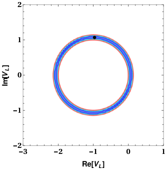
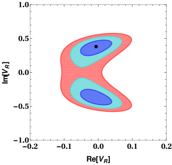
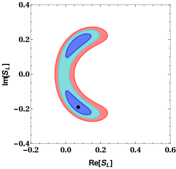
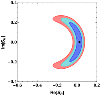
Figure 1: Constraints on real and imaginary parts of the new coefficients obtained from $R_{D^{(*)}}$, $R_{J/\psi}$, $R_{\pi}^{l}$, Br($B_{u,c}\to\tau\bar{\nu}_{\tau}$) and Br($B\to\pi\tau\bar{\nu}_{\tau}$) observables. Here the black dots represent the best-fit values.

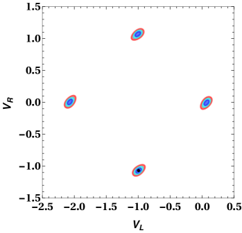
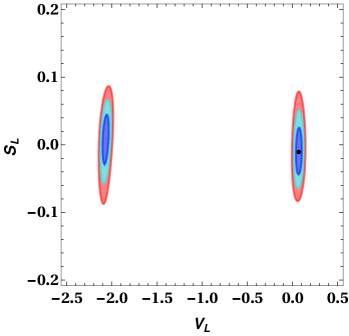
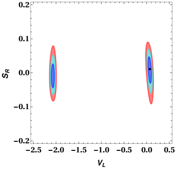
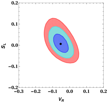
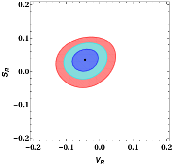
Figure 2: Constraints on new real coefficients obtained from $\chi^{2}$ fit to $R_{D^{(*)}}$, $R_{J/\psi}$, $R_{\pi}^{l}$, Br($B_{u,c}\to\tau\bar{\nu}_{\tau}$) and Br($B\to\pi\tau\bar{\nu}_{\tau}$) observables. Here the black dots represent the best-fit values.

Table 2: Best-fit, $\chi^{2}_{\rm min}/{\rm d.o.f}$ and pull values of new Wilson coefficients.

Cases	New Wilson coefficients	Best-fit values	$\chi^{2}_{\rm min}/{\rm d.o.f}$	Pull
Case A	$({\rm Re}[V_{L}],{\rm Im}[V_{L}])$	$(-0.9671,1.0723)$	$0.549$	$3.171$
	$({\rm Re}[V_{R}],{\rm Im}[V_{R}])$	$(-0.0062,0.3815)$	$0.543$	$3.1755$
	$({\rm Re}[S_{L}],{\rm Im}[S_{L}])$	$(0.0736,-0.188)$	$1.749$	$2.0134$
	$({\rm Re}[S_{R}],{\rm Im}[S_{R}])$	$(0.027,0)$	$2.1413$	$1.447$
Case B	$(V_{L},V_{R})$	$(-0.995,-1.07)$	$0.5425$	$3.176$
	$(V_{L},S_{L})$	$(0.072,-0.011)$	$0.506$	$3.205$
	$(V_{L},S_{R})$	$(0.069,0.01)$	$0.518$	$3.196$
	$(V_{R},S_{L})$	$(-0.052,0.0065)$	$1.886$	$1.836$
	$(V_{R},S_{R})$	$(-0.044,0.036)$	$1.409$	$3.0$
	$(S_{L},S_{R})$	$(0.0236,0.0575)$	$1.8415$	$1.9$

The constrained on various combination of real coefficients (case B), $V_{L}-V_{R}$ (top-left panel), $S_{L}-S_{R}$ (top-right panel), $V_{L}-S_{L}$ (middle-left panel), $V_{L}-S_{R}$ (middle-right panel), $V_{R}-S_{L}$ (bottom-left panel) and $V_{R}-S_{R}$ (bottom-right panel) obtained from $R_{D^{(*)}}$, $R_{J/\psi}$, $R_{\pi}^{l}$, Br($B_{u,c}\to\tau\bar{\nu}_{\tau}$) and Br($B\to\pi\tau\bar{\nu}_{\tau}$) observables are presented in Fig. 2 . Table 2 contains the best-fit values, $\chi^{2}_{\rm min}/{\rm d.o.f}$ and pull values of various sets of new real coefficients. It should be noticed that, the fit of $V_{L}-V_{R}$, $V_{L}-S_{L}$ and $V_{L}-S_{R}$ sets to all the $7$ observables are very well. However, the $V_{R}-S_{L}$, $V_{R}-S_{R}$ and $S_{L}-S_{R}$ sets provide very poor fit.

III $B_{c}\to D^{(*)}\tau\bar{\nu}_{\tau}$ DECAY OBSERVABLES

We discuss the branching ratio and angular observables of $B_{c}\to D^{(*)}\tau\bar{\nu}_{\tau}$ processes in this section. The branching ratios of $\bar{B}\to D\tau\bar{\nu}_{l}$ processes with respect to $q^{2}$ in the presence of new (pseudo)vector and (pseudo)scalar coefficients are given by Sakaki et al. (2013)

$$\frac{d\mathcal{BR}(\bar{B}\to Dl\bar{\nu}_{l})}{dq^{2}} = \tau_{B}{G_{F}^{2}|V_{cb}|^{2}\over 192\pi^{3}M_{B}^{3}}q^{2}\sqrt{\lambda_{D}(q^{2})}\left(1-{m_{l}^{2}\over q^{2}}\right)^{2}$$ (9)

$$\times\Bigg{\{}\Big{|}1+V_{L}+V_{R}\Big{|}^{2}\left[\left(1+{m_{l}^{2}\over 2q^{2}}\right)H_{0}^{2}+{3\over 2}{m_{l}^{2}\over q^{2}}H_{t}^{2}\right]$$

$$+{3\over 2}\left|S_{L}+S_{R}\right|^{2}\,H_{S}^{2}+3{\rm Re}\left[(1+V_{L}+V_{R})(S_{L}^{*}+S_{R}^{*})\right]{m_{l}\over\sqrt{q^{2}}}\,H_{S}H_{t}\Bigg{\}},$$

where

$$\lambda_{D}=\lambda(M_{B}^{2},M_{D}^{2},q^{2}),~{}~{}~{}~{}{\rm with}~{}~{}~{}~{}~{}\lambda(a,b,c)=a^{2}+b^{2}+c^{2}-2(ab+bc+ca)\,,$$ (10)

and $H_{i,\lambda}^{s}$’s ($\lambda=0,\pm,t$) are the heicity amplitudes. The branching ratios of $\overline{B}\to D^{*}\tau{\overline{\nu}}_{l}$ with respect to $q^{2}$ in the presence of new (pseudo)vector and (pseudo)scalar coefficients are given by are given by Sakaki et al. (2013)

$${d\mathcal{BR}(\bar{B}\to D^{*}l\bar{\nu}_{l})\over dq^{2}} = \tau_{B}{G_{F}^{2}|V_{cb}|^{2}\over 192\pi^{3}M_{B}^{3}}q^{2}\sqrt{\lambda_{D^{*}}(q^{2})}\left(1-{m_{l}^{2}\over q^{2}}\right)^{2}\times$$ (11)

$$\bigg{\{}\left(\left|1+V_{L}\right|^{2}+\left|V_{R}\right|^{2}\right)\left[\left(1+{m_{l}^{2}\over 2q^{2}}\right)\left(H_{V,+}^{2}+H_{V,-}^{2}+H_{V,0}^{2}\right)+{3\over 2}{m_{l}^{2}\over q^{2}}\,H_{V,t}^{2}\right]$$

$$-2{\rm Re}\left[\left(1+V_{L}\right)V_{R}^{*}\right]\left[\left(1+{m_{l}^{2}\over 2q^{2}}\right)\left(H_{V,0}^{2}+2H_{V,+}H_{V,-}\right)+{3\over 2}{m_{l}^{2}\over q^{2}}\,H_{V,t}^{2}\right]$$

$$+{3\over 2}|S_{L}-S_{R}|^{2}\,H_{S}^{2}+3{\rm Re}\left[\left(1+V_{L}-V_{R}\right)\left(S_{L}^{*}-S_{R}^{*}\right)\right]{m_{l}\over\sqrt{q^{2}}}\,H_{S}H_{V,t}\bigg{\}},$$

where $\lambda_{D^{*}}=\lambda(M_{B}^{2},M_{D^{*}}^{2},q^{2})$ $H_{i,\lambda}$’s are the helicity amplitudes.

Along with the branching ratios, we also explore the following observables in order to inspect the structure of new physics.

• $\tau$ forward-backward asymmetry

  $$\mathcal{A}_{\rm FB}^{D^{(*)}}={\int_{0}^{1}{d\Gamma\over d\cos{\theta}}d\cos{\theta}-\int^{0}_{-1}{d\Gamma\over d\cos{\theta}}d\cos{\theta}\over\int_{-1}^{1}{d\Gamma\over d\cos{\theta}}d\cos{\theta}}\,.$$ (12)

• Lepton non-universality

  $$R_{D^{(*)}}^{B_{c}}=\frac{{\mathcal{BR}}(B_{c}\to D^{(*)}\tau\bar{\nu}_{\tau})}{{\mathcal{BR}}(B_{c}\to D^{(*)}l\bar{\nu}_{l})},~{}~{}~{}~{}l=e,\mu.$$ (13)

• $\tau$ polarization asymmetry Sakaki et al. (2013)

  $$P_{\tau}^{D^{(*)}}(q^{2})=\frac{d\Gamma(\lambda_{\tau}=1/2)/dq^{2}-d\Gamma(\lambda_{\tau}=-1/2)/dq^{2}}{d\Gamma(\lambda_{\tau}=1/2)/dq^{2}+d\Gamma(\lambda_{\tau}=-1/2)/dq^{2}}\,.$$ (14)

• $D^{*}$ polarization asymmetry Biancofiore et al. (2013)

  $$F_{L,T}^{D^{*}}(q^{2})=\frac{d\Gamma_{L,T}\left(B_{c}\to D^{*}\tau\bar{\nu}\right)/dq^{2}}{d\Gamma\left(B_{c}\to D^{*}\tau\bar{\nu}\right)/dq^{2}}\,.$$ (15)

Like $R_{D^{(*)}}$ observables, the following fascinating observables (with the denominators involving only the light-lepton modes) are defined in Ref. Hu et al. (2019) .

• $\tau$ forward and backward fractions

  $$\chi_{1,2}^{D^{(*)}}=\frac{1}{2}R_{D^{(*)}}\left(1+A_{FB}^{D^{(*)}}\right)\,.$$ (16)

• $\tau$ spin $1/2$ and $-1/2$ fractions

  $$\chi_{3,4}^{D^{(*)}}=\frac{1}{2}R_{D^{(*)}}\left(1+P_{\tau}^{D^{(*)}}\right)\,.$$ (17)

• $D^{*}$ longitudinal and transverse polarization fractions

  $$\chi_{5,6}^{D^{*}}=R_{D^{*}}F_{L,T}^{D^{*}}\,.$$ (18)

IV NUMERICAL ANALYSIS AND EFFECT OF NEW COUPLINGS ON $B_{c}\to D^{(*)}\tau\bar{\nu}_{\tau}$ DECAY MODES

For numerical evaluation, we consider all the particle masses, life time of $B_{c}$ meson and CKM matrix elements from PDG Tanabashi et al. (2018) . The $q^{2}$ dependence of the $B_{c}\to D^{(*)}$ form factors is parametrized as

$$F(q^{2})=F(0)exp(c_{1}\hat{s}+c_{2}\hat{s}^{2})\,,~{}~{}~{}~{}~{}F=F_{+,0}^{B_{c}\to D},V^{B_{c}\to D^{*}},A_{0,1,2}^{B_{c}\to D^{*}}\,.$$ (19)

where $\hat{s}=s/M_{B_{c}}^{2}$ and the $F(0),c_{1},c_{2}$ coefficients that are obtained in the covariant light-front quark model are taken from Wang et al. (2009) .

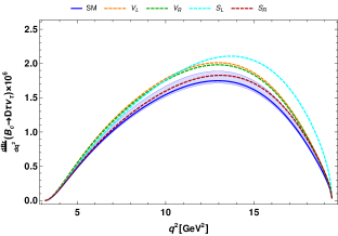
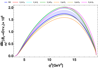
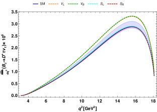
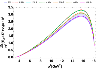
Figure 3: The variation of branching ratio of $B_{c}\to D\tau\nu_{\tau}$ (top panel) and $B_{c}\to D^{*}\tau\nu_{\tau}$ (bottom panel) processes with respect to $q^{2}$ for case A (left) and case B (right), respectively. Here the solid blue lines (lighter blues bands) represent the SM values (theoretical uncertainties obtained from input parameters). The orange, dark green, cyan and dark red colors stand for the additional complex $V_{L}$, $V_{R}$, $S_{L}$ and $S_{R}$ contributions, respectively. The red, cyan, dark green, orange, dark yellow and magenta colors are for the $(V_{L},V_{R})$, $(V_{L},S_{L})$, $(V_{L},S_{R})$, $(V_{R},S_{L})$, $(V_{R},S_{R})$ and $(S_{L},S_{R})$ sets of case B.

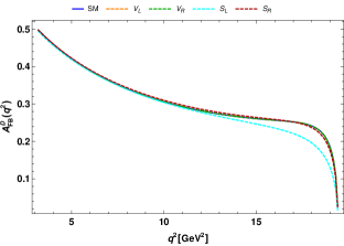
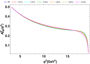
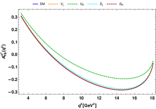
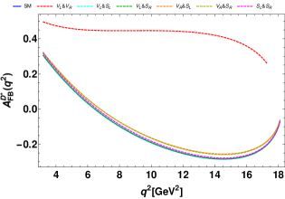
Figure 4: The $q^{2}$ variation of forward-backward asymmetry of $B_{c}\to D\tau\nu_{\tau}$ (top panel) and $B_{c}\to D^{*}\tau\nu_{\tau}$ (bottom panel) processes for case A (left) and case B (right), respectively.

Using the best-fit values of complex (real) Wilson coefficients from Table 2 , we show the $q^{2}$ variation of differential branching ratio ($\frac{d\mathcal{BR}}{dq^{2}}$), forward-backward asymmetry ($\mathcal{A}_{\rm FB}$), lepton non-universality ($R_{D^{(*)}}^{B_{c}}$), $\tau$ polarization asymmetry ($P_{\tau}^{D^{(*)}}$), $D^{*}$ longitudinal and transverse polarization ($F_{L,T}^{D^{*}}$), $\tau$ forward and backward fractions ($\chi_{1,2}^{D^{(*)}}$), $\tau$ spin $1/2$ and $-1/2$ fractions ($\chi_{3,4}^{D^{(*)}}$), $D^{*}$ longitudinal and transverse polarization fractions ($\chi_{5,6}^{D^{*}}$) of $B_{c}\to D\tau\bar{\nu}_{\tau}$ and $B_{c}\to D^{*}\tau\bar{\nu}_{\tau}$ decay modes in various Figures for both case A and case B.

In Fig. 3  the solid blue lines represent the SM central values and the lighter blue bands stand for the SM uncertainties which are obtained from the input parameters used in our analysis. Again, the orange, dark green, cyan and dark red colors are drawn by using the best-fit values of complex $V_{L}$, $V_{R}$, $S_{L}$ and $S_{R}$ coefficients, respectively for case A. Similarly, for case B, the red, cyan, dark green, orange, dark yellow and magenta colors stand respectively for real $(V_{L},V_{R})$, $(V_{L},S_{L})$, $(V_{L},S_{R})$, $(V_{R},S_{L})$, $(V_{R},S_{R})$ and $(S_{L},S_{R})$ combined sets of coefficients. We now wish to see how the differential branching ratios (${d\mathcal{BR}(\bar{B}\to D^{(*)}l\bar{\nu}_{l})\over dq^{2}}$), and other angular observables like $\mathcal{A}_{\rm FB}$, $R_{D^{(*)}}^{B_{c}}$, $P_{\tau}^{D^{(*)}}$, $F_{L,T}^{D^{*}}$, $\chi_{1,2}^{D^{(*)}}$, $\chi_{3,4}^{D^{(*)}}$, $\chi_{5,6}^{D^{*}}$ behave with different NP coefficients in both case A and case B.

In Fig. 3 we observe that the differential branching ratio is not affected by the presence of complex $S_{R}$ coefficient (top left panel), rather it lies within SM uncertainty blue band while both $V_{L}$ and $V_{R}$ coefficients show a small deviation in differential branching ratio, but the presence of complex $S_{L}$ coefficient provide significant deviation in the branching ratio of $B_{c}\to D\tau\bar{\nu}_{\tau}$ process where the peak of the distribution of differential branching ratio can shift to a higher $q^{2}$ region once the complex $S_{L}$ coefficient is introduced in case A. For case B, the differential branching ratio of $(B_{c}\to D\tau\bar{\nu}_{\tau})$ has deviated from the SM prediction for all possible sets of new coefficients except $(V_{R},S_{R})$ set of real coefficients while the peak can be shifted to a higher value $q^{2}$ for ($S_{L},S_{R})$ set of coefficients (top right panel) as shown in magenta color. Similarly the presence of complex $V_{L}$ and $V_{R}$ coefficients result in significant and identical deviation in differential branching ratio for $B_{c}\to D^{*}\tau\bar{\nu}_{\tau}$ decay (bottom-left panel) in case A while in case B, the sets of ($V_{L},V_{R}$), $(V_{L},S_{L})$ and $(V_{L},S_{R})$ sets of coefficients give remarkable deviation (bottom-right panel).

Fig. 4 depicts the forward-backward asymmetry of $B_{c}\to D\tau\bar{\nu}_{\tau}$ and $B_{c}\to D^{*}\tau\bar{\nu}_{\tau}$ decay modes with respect to $q^{2}$ in the top panel and bottom panel, respectively. We observe almost no deviation from SM predictions in the forward-backward asymmetry ($\mathcal{A}_{\rm FB}$) of $(B_{c}\to D\tau\bar{\nu}_{\tau})$ decay for both case A and case B, except a very little deviation for complex $S_{L}$ coefficient higher $q^{2}$ region. Therefore, one may conclude that the forward-backward asymmetry does not vary with any of the NP coefficients (except the complex $S_{L}$ cofficient) for $B_{c}\to D\tau\bar{\nu}_{\tau}$ decay, which is expected, since it is a ratio, the NP dependency gets canceled in the ratio. But the forward-backward asymmetry of $B_{c}\to D^{*}\tau\bar{\nu}_{\tau}$ process show profound deviation due to the presence of $V_{R}$ (bottom-left panel) in case A and $(V_{L},V_{R})$ set of real coefficients (bottom-right panel) in case B. Thus, we see the forward-backward asymmetry of $B_{c}\to D^{*}\tau\bar{\nu}_{\tau}$ decay process is very sensitive to $(V_{L},V_{R})$ set of coefficients. Again, we find $\mathcal{A}_{\rm FB}$ starts with peak value of 0.3 at low $q^{2}$ and becomes minimum with value -0.3 at $q^{2}=15\,$ GeV² and ends with value -0.05 at high $q^{2}$ in SM. Thus there is a zero crossing at $q^{2}=6.5\,$ GeV². However, in the presence of $(V_{L},V_{R})$ set of real coefficients (case B) there is no zero crossing and the value of forward-backward asymmetry lies between 0.5 at low $q^{2}$ and 0.3 at high $q^{2}$ as observed from bottom-right panel of Fig. 4.

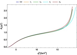
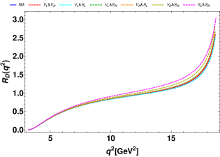
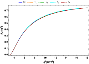
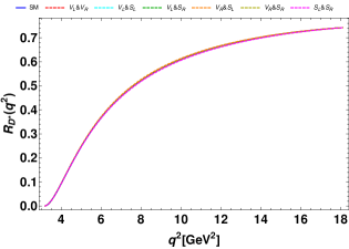
Figure 5: The variation of $R_{D}^{B_{c}}$ (top panel) and $R_{D^{*}}^{B_{c}}$ (bottom panel) parameters with respect to $q^{2}$ for case A (left) and case B (right), respectively.

The $q^{2}$ variation of the lepton non-universality parameters, $R_{D}^{B_{c}}$ and $R_{D^{*}}^{B_{c}}$ of $B_{c}\to D\tau\bar{\nu}_{\tau}$ and $B_{c}\to D^{*}\tau\bar{\nu}_{\tau}$ decay modes, for complex (left) and real (right) new coefficients are shown in the top and bottom panel respectively in Fig. 5 . Here, in top left panel, we see very little deviation from SM predictions in lepton non-universality parameter, $R_{D}^{B_{c}}$ of $B_{c}\to D\tau\bar{\nu}_{\tau}$ decay mode for complex $S_{L}$ coefficient in higher $q^{2}$ region (for $q^{2}>17$ Gev² ) in case A and for $(V_{R},S_{R})$, $(S_{L},S_{R})$ sets of real coefficients in case B (top right panel). Again, we want to emphasize the fact that the lepton non-universality parameter, $R_{D^{*}}^{B_{c}}$ of $B_{c}\to D^{*}\tau\bar{\nu}_{\tau}$ decay modes is not influenced by any of the NP coefficients in both case A and case B as observed in the bottom panel of Fig. 5 . It is worth mentioning that, the lepton non-universality parameter for both $B_{c}\to D\tau\bar{\nu}_{\tau}$ and $B_{c}\to D^{*}\tau\bar{\nu}_{\tau}$ decay modes, does not differ appreciably with the NP coefficients which is anticipated, because, the impact of NP coefficients gets canceled in the ratio of lepton non-universality parameter.

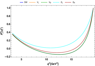
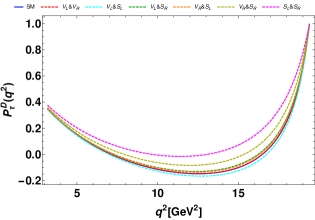
Figure 6: The $q^{2}$ variation of $\tau$ polarization asymmetry of $B_{c}\to D\tau\nu_{\tau}$ process for case A (left panel) and case B (right panel), respectively.

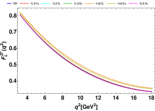
Figure 7: The $q^{2}$ variation of $D^{*}$ longitudinal (left panel) and transeverse (right panel) polarization asymmetry of $B_{c}\to D^{*}\tau\nu_{\tau}$ process for case B.

The $\tau$ longitudinal polarization asymmetry ($P_{\tau}^{D}$) of $B_{c}\to D\tau\nu_{\tau}$ decay mode with respect to $q^{2}$ in the presence of new complex (left panel) and real (right panel) coefficient are shown in Fig. 6 . We observe that the presence of only complex $S_{L}$ ($S_{R}$) coefficient in case A and the real $(S_{L},S_{R})$ ($(V_{R},S_{R})$) set of coefficients provide maximum deviation (small deviation) from the SM predictions in case B. Since there is no deviation in $P_{\tau}^{D^{*}}$ observable of $B_{c}\to D^{*}\tau\nu_{\tau}$ process from SM predictions, for both case A and case B, we do not include it as Figure. Similarly, $D^{*}$ longitudinal and transverse polarization ($F_{L,T}^{D^{*}}$) of $B_{c}\to D^{*}\tau\nu_{\tau}$ decay mode remains unchanged by the presence of complex $V_{L}$, $V_{R}$, $S_{L}$ and $S_{R}$ coefficients in case A, which is also excluded in this work. However, in case B, the $q^{2}$ variation of $F_{L,T}^{D^{*}}$ with longitudinal polarization asymmetry in left panel and transverse polarization asymmetry in right panel are shown in Fig. 7 . We see a small deviation in $F_{L,T}^{D^{*}}$ observable for $(V_{R},S_{L})$ and $(V_{R},S_{R})$ sets of real coefficients in case B.

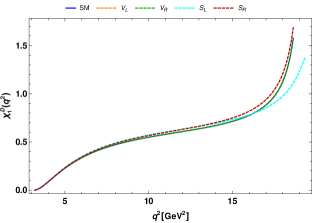
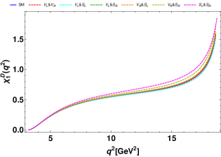
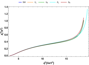
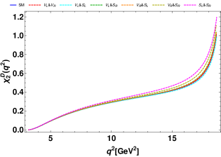
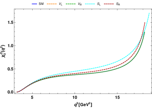
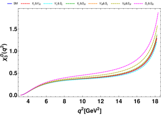
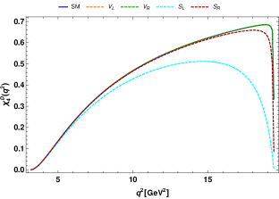
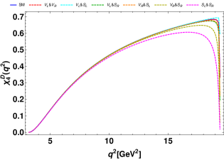
Figure 8: The $q^{2}$ variation of $\chi^{D}_{1,2,3,4}$ observables of $B_{c}\to D\tau\nu_{\tau}$ process for case A (left) and case B (right), respectively.

The variation $\tau$ forward and backward fractions ($\chi_{1,2}^{D}$) and $\tau$ spin $1/2$ and $-1/2$ fractions ($\chi_{3,4}^{D}$) of $B_{c}\to D\tau\nu_{\tau}$ decay mode with respect to $q^{2}$ in the presence of new complex and real coefficient are given in Fig. 8 . Here, the plots for $q^{2}$ distribution of $\chi_{1}^{D}$ (top), $\chi_{2}^{D}$ (second from top), $\chi_{1}^{D}$ (third from top) and $\chi_{4}^{D}$ (bottom) observables for case A (left panel) and case B (right panel) are shown. We notice that $q^{2}$ the distribution looks quite similar in $\chi_{1}^{D}$, $\chi_{2}^{D}$, $\chi_{3}^{D}$, that differs from $q^{2}$ the distribution of $\chi_{4}^{D}$ in both case A and case B. But the NP behaviour is quite similar in $\chi_{1,2,3,4}^{D}$ once we include the new Wilson coefficients in both case A and case B. Thus, in case A, the Wilson coefficient $S_{L}$ ($S_{R}$) causes significant (small) deviation from SM prediction, while in case B $(S_{L},S_{R})$ ($(V_{R},S_{R})$) set provides significant (small) deviation from SM prediction for $\chi_{1,2,3,4}^{D}$. Again, we want to point out the fact that, $\chi_{4}^{D}$ deviate profoundly from SM predictions, where the peak is shifted to lower $q^{2}$ region when we add complex $S_{L}$ coefficient in case A as is evident from bottom left panel of Fig. 8 .

The $\chi_{1,2,3,4,5,6}^{D^{*}}$ plots obtained by using the complex (case A) and real (case B) new Wilson coefficients are shown in Fig. 9 and 10 , respectively. In Fig. 9 and 10  the $q^{2}$ the distributions are different for $\chi_{1}^{D^{*}}$, $\chi_{2}^{D^{*}}$, $\chi_{3}^{D^{*}}$, $\chi_{5}^{D^{*}}$, but similar for $\chi_{4}^{D^{*}}$ and $\chi_{6}^{D^{*}}$. In Fig. 9, we observe small deviation in $\chi_{1}^{D^{*}}$, $\chi_{2}^{D^{*}}$ due to inclusion of the complex Wilson coefficient $V_{R}$ and in $\chi_{3}^{D^{*}}$, $\chi_{5}^{D^{*}}$ (very little) due to $S_{L}$ coefficient but, no deviation in $\chi_{4}^{D^{*}}$ and $\chi_{6}^{D^{*}}$ due to any of the complex coefficients for case A. Similarly, for case B, in Fig 10  we see $\chi_{1}^{D^{*}}$ and $\chi_{2}^{D^{*}}$ are seriously affected by $(V_{L},V_{R})$ set of real coefficients, $\chi_{5}^{D^{*}}$ and $\chi_{6}^{D^{*}}$ are very less affected by $(V_{R},S_{L})$, $(V_{R},S_{R})$ sets of coefficients, $\chi_{3}^{D^{*}}$ is negligibly affected only at the peak and $\chi_{4}^{D^{*}}$ is independent of all sets of real coefficients.

Table 3 and 4 contain the numerical values of the branching ratios and all the discussed angular observables of $B_{c}\to D\tau\nu_{\tau}$ and $B_{c}\to D^{*}\tau\nu_{\tau}$ decay processes in the presence of individual complex Wilson coefficient. The predicted values of branching ratio, forward-backward asymmetry, LNU parameters, $\tau$ and $D^{*}$ polarization asymmetry of $B_{c}\to D$ ($B_{c}\to D^{*}$) mode for case B are represented in Table 5 ( 6 ) .

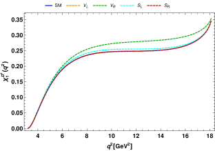
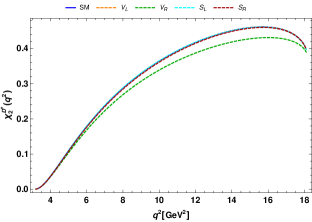
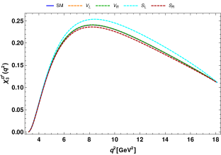
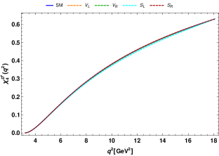
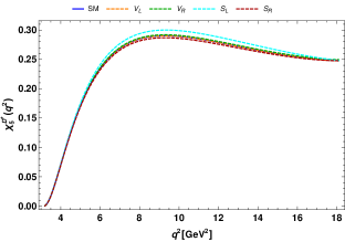
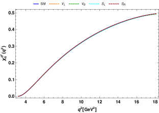
Figure 9: The $q^{2}$ variation of $\chi^{D^{*}_{1,2,3,4,5,6}}$ observables of $B_{c}\to D^{*}\tau\nu_{\tau}$ process for case A.

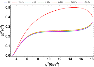
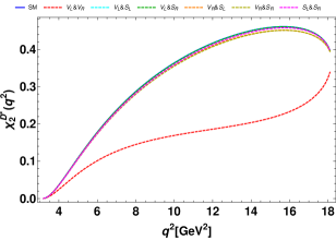
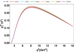
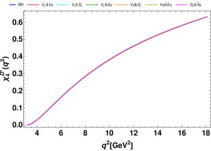
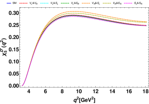
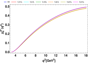
Figure 10: The $q^{2}$ variation of $\chi^{D^{*}_{1,2,3,4,5,6}}$ observables of $B_{c}\to D^{*}\tau\nu_{\tau}$ process for case B.

Table 3: Predicted numerical values of branching ratio and all the discussed angular observables of $B_{c}\to D\tau\nu_{\tau}$ process in the presence of individual complex Wilson coefficients.

Observables	Values in SM	Values in $V_{L}$	Values in $V_{R}$	Values in $S_{L}$	Values in $S_{R}$
$\rm{Br}(B_{c}\to D\tau\bar{\nu}_{\tau})\times 10^{5}$	$1.88\pm 0.131$	$2.165$	$2.132$	$2.282$	$1.972$
$\langle A_{FB}^{D}\rangle$	$0.295$	$0.295$	$0.295$	$0.28$	$0.296$
$\langle R_{D}\rangle$	$0.7$	$0.7$	$0.7$	$0.76$	$0.731$
$\langle P_{\tau}^{D}\rangle$	$-0.046$	$-0.046$	$-0.046$	$0.138$	$0.0023$
$\langle\chi_{1}^{D}\rangle$	$0.454$	$0.454$	$0.454$	$0.486$	$0.474$
$\langle\chi_{2}^{D}\rangle$	$0.247$	$0.247$	$0.247$	$0.274$	$0.257$
$\langle\chi_{3}^{D}\rangle$	$0.335$	$0.335$	$0.335$	$0.432$	$0.366$
$\langle\chi_{4}^{D}\rangle$	$0.367$	$0.367$	$0.367$	$0.328$	$0.365$

Table 4: Predicted numerical values of branching ratio and all the discussed angular observables of $B_{c}\to D^{*}\tau\nu_{\tau}$ process in the presence of individual complex Wilson coefficients.

Observables	Values in SM	Values in $V_{L}$	Values in $V_{R}$	Values in $S_{L}$	Values in $S_{R}$
$\rm{Br}(B_{c}\to D^{*}\tau\bar{\nu}_{\tau})\times 10^{5}$	$2.3\pm 0.161$	$2.65$	$2.66$	$2.33$	$2.292$
$\langle A_{FB}^{D^{*}}\rangle$	$-0.221$	$-0.221$	$-0.14$	$-0.211$	$-0.219$
$\langle R_{D^{*}}\rangle$	$0.603$	$0.603$	$0.603$	$0.608$	$0.601$
$\langle P_{\tau}^{D^{*}}\rangle$	$-0.41$	$-0.41$	$-0.41$	$-0.378$	$-0.418$
$\langle F_{L}^{D^{*}}\rangle$	$0.412$	$0.412$	$0.415$	$0.42$	$0.41$
$\langle F_{T}^{D^{*}}\rangle$	$0.588$	$0.588$	$0.585$	$0.58$	$0.59$
$\langle\chi_{1}^{D^{*}}\rangle$	$0.235$	$0.235$	$0.26$	$0.24$	$0.235$
$\langle\chi_{2}^{D^{*}}\rangle$	$0.368$	$0.368$	$0.344$	$0.368$	$0.366$
$\langle\chi_{3}^{D^{*}}\rangle$	$0.1782$	$0.1782$	$0.1784$	$0.189$	$0.175$
$\langle\chi_{4}^{D^{*}}\rangle$	$0.425$	$0.425$	$0.425$	$0.419$	$0.426$
$\langle\chi_{5}^{D^{*}}\rangle$	$0.249$	$0.249$	$0.25$	$0.26$	$0.246$
$\langle\chi_{6}^{D^{*}}\rangle$	$0.355$	$0.355$	$0.353$	$0.353$	$0.355$

Table 5: Predicted numerical values of branching ratio and all the angular observables of $B_{c}\to D\tau\nu_{\tau}$ process for case B.

Models	$\rm{Br}(B_{c}\to D\tau\bar{\nu}_{l})\times 10^{5}$	$\langle A_{FB}^{D}\rangle$	$\langle R_{D}\rangle$	$\langle P_{\tau}^{D}\rangle$	$\langle\chi_{1}^{D}\rangle$	$\langle\chi_{2}^{D}\rangle$	$\langle\chi_{3}^{D}\rangle$	$\langle\chi_{4}^{D}\rangle$
($V_{L},V_{R}$)	$2.134$	$0.295$	$0.7$	$-0.046$	$0.454$	$0.247$	$0.335$	$0.367$
($V_{L},S_{L}$)	$2.124$	$0.294$	$0.69$	$-0.065$	$0.446$	$0.244$	$0.323$	$0.367$
($V_{L},S_{R}$)	$2.185$	$0.2952$	$0.712$	$-0.028$	$0.461$	$0.251$	$0.346$	$0.366$
($V_{R},S_{L}$)	$1.712$	$0.295$	$0.71$	$-0.033$	$0.459$	$0.25$	$0.343$	$0.366$
($V_{R},S_{R}$)	$1.84$	$0.297$	$0.742$	$0.02$	$0.481$	$0.261$	$0.378$	$0.363$
($S_{L},S_{R}$)	$2.173$	$0.297$	$0.786$	$0.095$	$0.51$	$0.277$	$0.43$	$0.356$

Table 6: Predicted numerical values of branching ratio and all the angular observables of $B_{c}\to D^{*}\tau\nu_{\tau}$ process for case B.

Models	$\rm{Br}(B_{c}\to D^{*}\tau\bar{\nu}_{\tau})$	$\langle A_{FB}^{D^{*}}\rangle$	$\langle R_{D^{*}}\rangle$	$\langle P_{\tau}^{D^{*}}\rangle$	$\langle F_{L}^{D^{*}}\rangle$	$\langle\chi_{1}^{D}\rangle$	$\langle\chi_{2}^{D}\rangle$	$\langle\chi_{3}^{D}\rangle$	$\langle\chi_{4}^{D}\rangle$	$\langle\chi_{5}^{D}\rangle$	$\langle\chi_{6}^{D}\rangle$
($V_{L},V_{R}$)	$2.652\times 10^{-5}$	$0.4$	$0.603$	$-0.41$	$0.414$	$0.421$	$0.182$	$0.178$	$0.425$	$0.25$	$0.353$
($V_{L},S_{L}$)	$2.64\times 10^{-5}$	$-0.222$	$0.602$	$-0.412$	$0.41$	$0.234$	$0.368$	$0.177$	$0.425$	$0.248$	$0.352$
($V_{L},S_{R}$)	$2.62\times 10^{-5}$	$-0.22$	$0.602$	$-0.412$	$0.41$	$0.235$	$0.368$	$0.177$	$0.425$	$0.25$	$0.355$
($V_{R},S_{L}$)	$2.49\times 10^{-5}$	$-0.195$	$0.61$	$-0.4$	$0.437$	$0.244$	$0.36$	$0.18$	$0.425$	$0.264$	$0.341$
($V_{R},S_{R}$)	$2.44\times 10^{-5}$	$-0.197$	$0.602$	$-0.417$	$0.43$	$0.242$	$0.36$	$0.175$	$0.426$	$0.259$	$0.343$
($S_{L},S_{R}$)	$2.3\times 10^{-5}$	$-0.215$	$0.6$	$-0.42$	$0.41$	$0.236$	$0.365$	$0.174$	$0.426$	$0.246$	$0.355$

V Conclusion

In this paper, we have investigated $B_{c}\to D^{(*)}\tau\bar{\nu}_{\tau}$ semileptonic decays mediated by $b\to u\tau\nu_{\tau}$ quark level transitions in an effective field theory approach. We consider the presence of an additional vector and scalar type interactions which can be either complex or real catagorized as two cases. In case A, existence of only individual new complex coefficient and case B, existence of only two new real coefficients and we perform a chi-square fitting to extract the best-fit values of these new Wilson coefficients from the experimental data on $R_{D^{(*)}}$, $R_{J/\psi}$, $R_{\pi}^{l}$, Br($B_{u,c}\to\tau\bar{\nu}_{\tau}$) and Br($B\to\pi\tau\bar{\nu}_{\tau}$) observables. We estimate the branching ratio, forward-backward asymmetry ($\mathcal{A}_{\rm FB}$), lepton non-universality ($R_{D^{(*)}}^{B_{c}}$), $\tau$ polarization asymmetry ($P_{\tau}^{D^{(*)}}$), $D^{*}$ longitudinal and transverse polarization ($F_{L,T}^{D^{*}}$), $\tau$ forward and backward fractions ($\chi_{1,2}^{D^{(*)}}$), $\tau$ spin $1/2$ and $-1/2$ fractions ($\chi_{3,4}^{D^{(*)}}$), $D^{*}$ longitudinal and transverse polarization fractions ($\chi_{5,6}^{D^{*}}$) of $B_{c}\to D\tau\bar{\nu}_{\tau}$ and $B_{c}\to D^{*}\tau\bar{\nu}_{\tau}$ decay modes for both case A and case B using the best-fit values of real and complex Wilson coefficients.

The presence of complex $S_{L}$ coefficient provide significant deviation from SM prediction in the differential branching ratio of $B_{c}\to D\tau\bar{\nu}_{\tau}$ process, where the peak of the distribution of differential branching ratio can shift to a higher $q^{2}$ region, while $V_{L}$, $V_{R}$ coefficients show a small deviation, and $S_{R}$ coupling results in no deviation for case A. For case B, the differential branching ratio of $(B_{c}\to D\tau\bar{\nu}_{\tau})$ has deviated from the SM prediction for all possible sets of new coefficients except $(V_{R},S_{R})$ set of real coefficients while the peak can be shifted to a higher value $q^{2}$ for ($S_{L},S_{R})$ set of coefficients. Similarly the presence of complex $V_{L}$ and $V_{R}$ coefficients result in significant deviation in differential branching ratio for $B_{c}\to D^{*}\tau\bar{\nu}_{\tau}$ decay in case A while in case B, the sets of ($V_{L},V_{R}$), $(V_{L},S_{L})$ and $(V_{L},S_{R})$ coefficients give significant deviation.

We find almost no deviation from SM predictions in forward backward asymmetry for $B_{c}\to D\tau\bar{\nu}_{\tau}$ decay for both case A and case B except a very little deviation for complex $S_{L}$ coefficient higher $q^{2}$ region. This is expected, since it is a ratio, the NP dependency gets canceled in the ratio. But the forward-backward asymmetry of $B_{c}\to D^{*}\tau\bar{\nu}_{\tau}$ process show profound deviation due to the presence of $V_{R}$ in case A and $(V_{L},V_{R})$ coefficients in case B.

The lepton non-universality parameter, $R_{D}^{B_{c}}$ of $B_{c}\to D\tau\bar{\nu}_{\tau}$ decay process is deviated slightly for complex $S_{L}$ coefficient in higher $q^{2}$ region in case A and for $(V_{R},S_{R})$, $(S_{L},S_{R})$ real coefficients in case B. But, $R_{D^{*}}^{B_{c}}$ of $B_{c}\to D^{*}\tau\bar{\nu}_{\tau}$ decay mode is not influenced by any of the NP coefficients in both case A and case B. It is worth mentioning that, the lepton non-universality parameter for both $B_{c}\to D\tau\bar{\nu}_{\tau}$ and $B_{c}\to D^{*}\tau\bar{\nu}_{\tau}$ decay modes, does not differ significantly with the NP coefficients as anticipated, because, the impact of NP coefficients gets canceled in the ratio of lepton non-universality parameter.

In the $\tau$ longitudinal polarization asymmetry ($P_{\tau}^{D}$) of $B_{c}\to D\tau\nu_{\tau}$ process, the presence of only complex $S_{L}$ in case A and the real $(S_{L},S_{R})$ set provide maximum deviation from the SM predictions in case B. There is no deviation in $P_{\tau}^{D^{*}}$ observable of $B_{c}\to D^{*}\tau\nu_{\tau}$ process from SM predictions, for both case A and case B. Similarly, $D^{*}$ longitudinal and transverse polarization ($F_{L,T}^{D^{*}}$) of $B_{c}\to D^{*}\tau\nu_{\tau}$ decay mode is independent of all complex coefficients in case A. However, longitudinal and transverse polarization asymmetry ($F_{L,T}^{D^{*}}$) slightly deviated from SM prediction for $(V_{R},S_{L})$ and $(V_{R},S_{R})$ sets of new coefficients in case B.

Again, the spin $1/2$ and $-1/2$ fractions, $\chi_{4}^{D}$ of $B_{c}\to D\tau\nu_{\tau}$ decay mode deviate profoundly from SM predictions due to complex $S_{L}$ coefficient, where the peak is shifted to lower $q^{2}$ region in case A and due to real $(S_{L},S_{R})$ set of coefficients in case B. In $B_{c}\to D^{*}\tau\nu_{\tau}$ decay, we observe small deviation in $\chi_{1}^{D^{*}}$, $\chi_{2}^{D^{*}}$ due to inclusion of the complex Wilson coefficient $V_{R}$ and no deviation in $\chi_{4}^{D^{*}}$ and $\chi_{6}^{D^{*}}$ due to any of the complex coefficients for case A. Similarly, for case B, we see $\chi_{1}^{D^{*}}$ and $\chi_{2}^{D^{*}}$ are seriously affected by $(V_{L},V_{R})$ set of real coefficients and $\chi_{4}^{D^{*}}$ is independent of all sets of real coefficients.

The observables associated with $B_{c}\to D\tau\nu_{\tau}$ decay mode like differential branching ratio, forward backward asymmetry ($\mathcal{A}_{\rm FB}$), lepton non-universality parameter ($R_{D}^{B_{c}}$), $\tau$ longitudinal polarization asymmetry ($P_{\tau}^{D}$), spin $1/2$ and $-1/2$ fractions ($\chi_{4}^{D}$) are found to be mostly affected by complex $S_{L}$ coefficient in case A and real $(S_{L},S_{R})$ set of coefficients in case B. Similarly $B_{c}\to D^{*}\tau\nu_{\tau}$ decay, the observables differential branching ratio, forward backward asymmetry, $\chi_{1}^{D^{*}}$ and $\chi_{2}^{D^{*}}$ are influenced by complex $V_{R}$ coefficient while lepton non-universality parameter, $\chi_{4}^{D^{*}}$ and $\chi_{6}^{D^{*}}$ do not depend on any of the real cefficients in case A. In case B, forward backward asymmetry, $\chi_{1}^{D^{*}}$ and $\chi_{2}^{D^{*}}$ are seriously affected by $(V_{L},V_{R})$ set of real coefficients, but lepton non-universality parameter, $\chi_{4}^{D^{*}}$ are independent of all sets of real coefficients

At present, there exist a few measurements of $B_{c}$ meson and its properties from Tevatron data. The LHCb experiments assure the first detailed study of $B_{c}$ meson. More precise measurements of its mass and lifetime are now feasible, and several decay channels have been witnessed for the first time. LHCb experiment will provide additional information with significant reduction of the uncertainties of the observables already measured and measurement of new observables that can provide complementary information on lepton flavor universality violation and the NP coefficients, thus we expect a better understanding of the different NP scenarios involved in $b\to u\tau\nu_{\tau}$ transitions