Competing flow and collision effects in a monodispersed liquid-solid fluidized bed at a moderate Archimedes number

Abstract

We study the effects of fluid-particle and particle-particle interactions in a three-dimensional monodispersed reactor with unstable fluidization. Simulations were conducted using the Immersed Boundary Method (IBM) for particle Reynolds numbers of 20-70 with an Archimedes number of 23600. Two different flow regimes were identified as a function of the particle Reynolds number. For low particle Reynolds numbers ($20<Re_{p}<40$), the porosity is relatively low and the particle dynamics are dominated by interparticle collisions that produce anisotropic particle velocity fluctuations. The relative importance of hydrodynamic effects increases with increasing particle Reynolds number, leading to a minimized anisotropy in the particle velocity fluctuations at an intermediate particle Reynolds number. For high particle Reynolds numbers ($Re_{p}>40$), the particle dynamics are dominated by hydrodynamic effects, leading to decreasing and more anisotropic particle velocity fluctuations. A sharp increase in the anisotropy occurs when the particle Reynolds number increases from 40 to 50, corresponding to a transition from a regime in which collision and hydrodynamic effects are equally important (Regime 1) to a hydrodynamic-dominated regime (Regime 2). The results imply an optimum particle Reynolds number of roughly 40 for the investigated Archimedes number of 23600 at which mixing in the reactor is expected to peak, which is consistent with reactor studies showing peak performance at a similar particle Reynolds number and with a similar Archimedes number. Results also show that maximum effective collisions are attained at intermediate particle Reynolds number. Future work is required to relate optimum particle Reynolds number to Archimedes number.

1 Introduction

Fluidization has been widely found in many industrial processes such as water and wastewater treatment and chemical synthesis. In these processes, one of the key operating parameters is the flow rate which in turn controls the porosity to achieve efficient mixing and mass transfer. Depending on the processes, the optimal operating parameter can vary significantly. By gaining a detailed understanding of the particle dynamics in the fluidized bed, system optimization would be possible. Using wastewater treatment as an illustrative example, the Staged Anaerobic Fluidized-bed Membrane Bioreactor (SAF-MBR) was recently proposed to reduce energy demand (Shin et al., 2011, 2012, 2014) in which granular activated carbon (GAC) particles are fluidized to both maximize biological degradation rate through maximizing the growth of biofilm and minimize membrane fouling through particle collisions. Both objectives can be optimized by choosing the optimal flow rate which in turn controls the porosity. In addition to operation, elucidating the particle dynamics in fluidized bed can provide information to model biofilm detachment rate. Important biofilm detachment mechanisms include shear stress from fluid-particle interactions and abrasion from particle-particle interactions (Rittmann & McCarty, 2018; Nicolella et al., 1996, 1997). However, the proposed models either fail to decouple effect of shear stress from abrasion or only consider abrasion effects (Chang et al., 1991; Nicolella et al., 1997; Gjaltema et al., 1997). Without a thorough understanding of the particle dynamics, especially the competition between abrasion and hydrodynamic effects in the fluidized bed, optimizing operating parameters for efficient mixing and modeling biofilm detachment remains an elusive problem.

In the past few decades, many researchers have studied the hydrodynamics of fluidized-bed reactors (Verma et al., 2014, 2015; Lu et al., 2020; Yang et al., 2017; Zenit et al., 1997; Duru et al., 2002; Derksen & Sundaresan, 2007; Di Felice, 1999; Shajahan & Breugem, 2020). In general, fluidized beds are classified into two different categories as either aggregative or particulate (Geldart, 1973). The behavior of fluidized beds can be further classified based on the Froude number $Fr_{m}=u_{mf}^{2}/(gd_{p})$, where $u_{mf}$ is the minimum fluidization velocity, $g$ is the gravitational acceleration and $d_{p}$ is the particle diameter (Sundaresan, 2003). For $Fr_{m}\sim\mathcal{O}(10^{-3})$, no bubbles are observed. For $Fr_{m}\sim\mathcal{O}(10^{-2})$, bubbles appear intermittently. For $Fr_{m}\sim\mathcal{O}(10^{-1})$, bubble-like voids persist. In wastewater treatment, $Fr_{m}\sim\mathcal{O}(10^{-3})$ is generally assumed based on the particles used (Shin et al., 2014). Zenit et al. (1997) measured the particle pressure (collision stress) for particles with different properties over a range of volume fractions and showed that the particle pressure initially increases with decreasing volume fraction when the volume fraction is large and then decreases with further decreasing volume fraction, an effect that was also demonstrated by Derksen & Sundaresan (2007). Since particle pressure measures the effect of collisions, it can be used to quantify abrasion that leads to biofilm detachment. Although they did not directly quantify hydrodynamic stresses, Derksen & Sundaresan (2007) attempted to evaluate the importance of particle streaming stress which is a measure of the hydrodynamic pressure induced by particle velocity fluctuations. Yao et al. (2021b) studies the effect of Archimedes number in concentrated suspensions and discovers that low Archimedes number suspensions result in long-lived particle clusters while high Archimedes number suspensions mainly consist of short-lived particle clusters.

To elucidate the effect of porosity on particle dynamics in the AFBR, we study the fluid-particle and particle-particle interactions in a fluidized bed with the Eulerian-Lagrangian (EL) method. EL methods solve for the dynamics of individual particles and compute the Eulerian flow-discrete particle and particle-particle interactions with different collision models (Yu & Xu, 2003; Akiki et al., 2016; Costa et al., 2015; Biegert et al., 2017). EL methods can be further classified into two sub-categories: (i) Volume-averaged Computational Fluid Dynamics-Discrete Element Methods (CFD-DEM) and (ii) Particle Resolved Simulations (PRS). The CFD-DEM method employs various closure laws to model the momentum transfer between the discrete particles and the fluid (Yu & Xu, 2003; Pan et al., 2016). One advantage of CFD-DEM is its ability to simulate millions of particles, as in the study of the macroscopic behavior of particle-laden flows leading to clustering (Akiki et al., 2017a, b). However, there is no consensus on the most appropriate closure laws to parameterize the fluid-particle interactions (Yin & Koch, 2007; Tenneti et al., 2011). Another disadvantage is that the Eulerian fields are volume averaged which precludes statistical analysis of motions related to detailed fluid-particle interactions.

Because of the need for closure laws in CFD-DEM, it cannot be used to study the detailed physics of fluid-particle and particle-interactions in an AFBR. Therefore, we employ the PRS approach which can be thought of as the limiting case of the CFD-DEM method in which the Eulerian flow is computed on a grid in which many (15-30) grid cells resolve the smallest particle diameter to simulate all of the spatio-temporal scales related to the flow-particle interactions (Esteghamatian et al., 2017; Lee et al., 2011; Lee & Balachandar, 2010). As a result, the Eulerian quantities are no longer volume-averaged over many particles, which allows for a direct quantification of particle dynamics in systems like fluidized-bed reactors. Three popular approaches used to study particle-laden flows are the PHYSALIS method (Zhang & Prosperetti, 2005), the Immersed Boundary Method (IBM), and the Lattice-Boltzmann (LB) technique with comparable accuracy (Finn & Apte, 2013). Recently, the PRS approach with IBM has been widely applied to a number of different problems, including extracting drag laws from arrays of particles (Tenneti et al., 2011; Akiki et al., 2017b; Tang et al., 2015) and understanding the detailed physics of flow-particle interactions in fluidized beds and particle suspensions (Esteghamatian et al., 2017; Kriebitzsch et al., 2013; Yin & Koch, 2007; Willen & Prosperetti, 2019; Ozel et al., 2017; Uhlmann & Doychev, 2014; Zaidi et al., 2015).

In this paper, we present PRS results of a fluidized bed reactor to gain a detailed understanding of the effects of varying upflow velocity on the particle dynamics. A series of cases with different particle Reynolds numbers is studied and the simulation results are used to (1) understand the equilibrium behavior of particle fluctuations, (2) establish links between particle velocity fluctuations, forces on particles and flow-particle microstructure and (3) identify various flow regimes and momentum transfer mechanisms as a function of the particle Reynolds number.

2 Numerical methodology

2.1 Equations and discretizations

The governing Navier-Stokes equations are solved in a three-dimensional flow reactor with a square cross section and with an array of uniform spherical particles. Direct forcing by the IBM method is accounted for with a source term, $\boldsymbol{f}_{IBM}$, which is added to the Navier-Stokes equation and enforces no-slip boundary conditions on the particle surfaces. With this forcing, the incompressible Navier-Stokes equation we solve is given by

$$\partialderivative{\boldsymbol{u}}{t}+\boldsymbol{u}\dotproduct\gradient{\boldsymbol{u}}=-\gradient{p}+\nu\laplacian{\boldsymbol{u}}+\boldsymbol{f}_{IBM},$$ (1)

subject to continuity, $\divergence{\boldsymbol{u}}=0$, where $\boldsymbol{u}$ is the velocity vector and $p$ is the pressure normalized by the fluid density, $\rho_{f}$. These equations are discretized on a uniform collocated Cartesian grid and momentum and pressure are coupled with the fractional step method (Zang et al., 1994). The advection term is discretized with the explicit, three-step Runge-Kutta schemes described in Rai & Moin (1991). The viscous term is discretized with the implicit Crank-Nicolson scheme to eliminate the associated stability constraints.

The IBM formulation employs the direct forcing approach first proposed by Uhlmann (2005) and improved by Kempe & Fröhlich (2012a). This approach represents the particle using $N_{L}$ Lagrangian markers with volume $\Delta{V}_{L}\approx\Delta{V}_{E}$, where $\Delta{V}_{L}$ is the Lagrangian marker volume and $\Delta{V}_{E}$ is the volume of each Eulerian grid cell. At each time step, the IBM force, $\boldsymbol{f}_{IBM}$, is calculated as the force required to enforce the difference between the desired velocity ${\bf u}_{d}$ at the particle surface and the interpolated velocity from the Eulerian grid. The desired velocity at the particle surface is calculated as the sum of a translational (${\bf u}_{p}$) and a rotational components based on the particle angular velocity vector ${\bf\omega}_{p}$ with ${\bf u}_{d}={\bf u}_{p}+{\bf\omega}_{p}\times{\bf r}$, where ${\bf r}$ is the vector pointing from the particle center of mass to the Lagrangian point. The translational and angular velocities of the particle are then governed by

$$m_{p}\derivative{\boldsymbol{u}_{p}}{t} = \rho_{f}\Big{[}\derivative{t}\int_{\Omega_{p}}\boldsymbol{u}\ \differential\Omega_{p}-\int_{S}\boldsymbol{f}_{IBM}\ \differential S\Big{]}+V_{p}(\rho_{p}-\rho_{f})\boldsymbol{g}+\boldsymbol{F}_{c,p},$$ (2a)

$$I_{p}\derivative{\boldsymbol{\mathbf{\omega}}_{p}}{t} = \rho_{f}\Big{[}\derivative{t}\int_{\Omega_{p}}\boldsymbol{r}\times\boldsymbol{u}\ \differential\Omega_{p}-\int_{S}\boldsymbol{r}\times\boldsymbol{f}_{IBM}\ \differential S\Big{]}+\boldsymbol{T}_{c,p},$$ (2b)

where the integrals are calculated over the discrete volumes associated with the Lagrangian points given by the surface $S$ and region $\Omega_{p}$, $m_{p}$ is the mass of the particle, $\boldsymbol{g}$ is the gravitational acceleration vector which points in the negative z-direction, $V_{p}$ is the volume of the particle, $\rho_{p}$ is the particle density, $\boldsymbol{F}_{c,p}$ and $\boldsymbol{T}_{c,p}$ are the force and torque due to particle-particle and particle-wall interactions, and $I_{p}$ is the moment of inertia of the particle. For a description of each term in equations (2), please refer to the papers by Uhlmann (2005) and Kempe & Fröhlich (2012a). Interpolation of variables between the Lagrangian and Eulerian grid employs the discrete delta function kernel proposed by Peskin (1977) and Roma et al. (1999).

The original direct forcing approach proposed by Uhlmann (2005) has two disadvantages: (1) the rigid-body approximation used to approximate the volume integral, $\derivative{t}\int_{\Omega_{p}}\rho_{f}\boldsymbol{u}\ \differential\Omega_{p}$ in equation (2) introduces a singularity at density ratio of $\rho_{p}/\rho_{f}=1$ and stability limit of $\rho_{p}/\rho_{f}\approx 1.2$ (Uhlmann, 2005; Kempe & Fröhlich, 2012a) and (2) the explicit calculation of $\boldsymbol{f}_{IBM}$ leads to error that is inversely proportional to $Re_{p}$ and cannot be eliminated by refining the time step (Kempe & Fröhlich, 2012a). The restriction associated with the rigid-body approximation is eliminated by introducing the numerical level-set approximation of the volume integral in equation (2) instead of applying the rigid-body approximation. The error associated with $\boldsymbol{f}_{IBM}$ is reduced by applying a heuristic number of outer forcing loops (Kempe & Fröhlich, 2012a; Wang et al., 2008). In each outer forcing loop, the Eulerian velocity field is interpolated between the Eulerian and Lagrangian grid and updated with the newly calculated $\boldsymbol{f}_{IBM}$ to satisfy the no-slip boundary condition at the particle surface. Details can be found in the paper by Kempe & Fröhlich (2012a), who recommended three outer forcing loops while Biegert et al. (2017) recommended one loop based on various validation cases. After validating with different cases, two outer forcing loops were used for the simulations in this study.

To model the forces associated with particle-particle and particle-wall interactions, the total force and torque on particle $p$ due to interaction with $q=1,2,\dots,N_{p}$ particles and a wall $w$ are computed with

$$\boldsymbol{F}_{c,p} = \sum_{p,q\neq p}^{N_{p}}(\boldsymbol{F}_{n,q}+\boldsymbol{F}_{t,q})+\boldsymbol{F}_{n,w}+\boldsymbol{F}_{t,w},$$ (3a)

$$\boldsymbol{T}_{c,p} = \sum_{p,q\neq p}^{N_{p}}R_{p,cp}\boldsymbol{n}_{p,q}\times\boldsymbol{F}_{t,q}+R_{p,cp}\boldsymbol{n}_{p,w}\times\boldsymbol{F}_{t,w},$$ (3b)

where $\boldsymbol{F}_{n,q}$ and $\boldsymbol{F}_{t,q}$ are the normal and tangential collision forces between particle $p$ and $q$, $\boldsymbol{F}_{n,w}$ and $\boldsymbol{F}_{t,w}$ are the normal and tangential collision forces between particle $p$ and a wall, $R_{p,cp}$ is the effective radius between particle $p$ and $q$, $\boldsymbol{n}_{p,q}$ is the vector normal to the plane of contact between particles $p$ and $q$, and $\boldsymbol{n}_{p,w}$ is the vector normal to the wall at the point of contact with particle $q$. Normal collision forces $\boldsymbol{F}_{n,q}$ consist of contributions from both lubrication and contact based on the separation distance between the particles (Biegert et al., 2017). Collision models usually have high stiffness in which the collision time step size is much smaller than the fluid time step size. To avoid this, we follow the approach by Biegert et al. (2017) who employ the collision model proposed by Kempe & Fröhlich (2012b).

The code we employ for the simulations in this paper is based on the code developed by Drs. Hyungoo Lee and Sivaramakrishnan Balachandar, who employed IBM with the direct forcing approach by Uhlmann (2005) to simulate the near-wall motion of an isolated particle (Lee & Balachandar, 2010; Lee et al., 2011). We modified their code following improvements to the IBM method suggested by Kempe & Fröhlich (2012a) and Biegert et al. (2017) as follows. To improve the accuracy of computing fluid-solid interactions, the following modifications were made: 1) Three-step Runge-Kutta time-stepping scheme instead of third-order Adams-Bashforth for the advection terms in equation (1), 2) Outer forcing loops to reduce the error associated with explicit calculation of the forcing in the IBM method (Kempe & Fröhlich, 2012a) and 3) Higher-order schemes with predictor and corrector steps to discretize the particle motion equations (equation 2) (Biegert et al., 2017). Because the original code was not designed to simulate particle-particle interactions, collision models based on Kempe & Fröhlich (2012b) and Biegert et al. (2017) were implemented. Finally, computational performance was made efficient by 1) using appropriate MPI (Open MPI-3.0) structures to transfer Lagrangian and Eulerian information related to particle-particle collisions at interprocessor boundaries 2) employing Hypre libraries developed at the Lawrence Livermore National Laboratories (Falgout, 2006; Chow et al., 1998) to solve the linear systems associated with implicit discretization of the viscous terms and the pressure-Poisson equation.

3 Fluidized bed simulation setup

To simulate the fluidized bed, three-dimensional simulations are conducted with $N_{p}=2000$ particles in the reactor channel shown in figure 1. The particles have a uniform diameter $d_{p}=2$ mm and density $\rho_{p}=1300$ kg m^-3, and the fluid has a kinematic viscosity $\nu=10^{-6}$ m² s^-1 and density $\rho_{f}=998.21$ kg m^-3, resulting in Archimedes number $Ar=23600$ (Galileo number $Ga=154$) that is defined as

$$Ar=Ga^{2}=\dfrac{g(s-1)d_{p}^{3}}{\nu^{2}},$$ (4)

where $s=\rho_{p}/\rho_{f}$ is the ratio of particle to fluid density. The particle collisions have a dry restitution coefficient $e_{dry}=0.97$ (Joseph et al., 2001; Foerster et al., 1994), coefficient of kinetic friction $\mu_{k}=0.15$ (Joseph & Hunt, 2004) and coefficient of static friction $\mu_{s}=0.8$ (Dieterich, 1972). The grid spacing is uniform in the $x$, $y$ and $z$ directions and given by $\Delta x=\Delta y=\Delta z=h=d_{p}/25.6$, which is sufficient to resolve the flow-particle interactions (Biegert, 2018; Kempe & Fröhlich, 2012a). The channel width is given by $L_{x}=L_{y}=10d_{p}$ and its length is $L_{z}=60d_{p}$, giving a three-dimensional grid with 256$\times$256$\times$1536 grid points. The time-step size is $\Delta{t}=1.5\times 10^{-4}$ s, resulting in a maximum Courant number of $0.5$ for the cases with the highest upflow velocities.

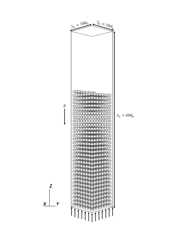
Figure 1: The three-dimensional computational domain, showing the fluidized bed, the uniform inflow velocity profile and the initial particle positions.

The primary parameter of interest is the particle Reynolds number $Re_{p}=u_{0}d_{p}/\nu$, where the average upflow velocity at the inlet, $u_{0}$, is varied to investigate Reynolds number effects. Cases are run with periodicity in the $x$ and $y$ directions. A total of six simulations were conducted with $0.010\leq u_{0}\leq 0.035$ m s^-1, giving $20\leq Re_{p}\leq 70$. For all cases, the pressure is specified at the top boundary as $p=0$, while at the bottom boundary the inflow velocity is specified as uniform and given by $w(x,y)=u_{0}$.

Simulations are initialized with a uniform distribution of particles with a spacing of $1d_{p}$ and the flow is impulsively started from rest. The upflow velocity leads to expansion of the bed and random motion of the particles until statistical equilibrium is reached, at which time the dynamics are independent of the initial particle distribution.

4 Results and discussion

4.1 Instantaneous and time-average porosity

To understand the time evolution of the particles, we define the ensemble-average instantaneous vertical velocity of particles using the ensemble-average

$$\langle\langle\{\cdot\}\rangle\rangle=\dfrac{1}{N_{p}}\sum_{i=1}^{N_{p}}\{\cdot\}_{i},$$ (5)

where $\{\cdot\}_{i}$ corresponds to the variable of particle $i$. As shown in figure 2(a), the ensemble-averaged instantaneous vertical velocity of particles $\langle\langle w_{p}\rangle\rangle$ initially increases with time as the bed expands because the average drag force on the particles exceeds their submerged weight. Eventually, the average drag is in balance with the submerged weight, leading to statistical equilibrium. Defining the particle turnover time as $\tau_{T}=d_{p}/u_{0}$, simulations are run for $t_{max}=100-300\tau_{T}$, depending on $Re_{p}$, to ensure statistically-stationary results. Time-averaged statistics are denoted by the overbar and computed over the last 80 turnover times, such that

$$\overline{\{\cdot\}}=\frac{1}{80\tau_{T}}\int_{t_{0}}^{t_{\max}}\{\cdot\}\,\differential t\,,$$ (6)

where $t_{0}=t_{\max}-80\tau_{T}$. Unless otherwise stated, the time-averaging operator has been applied to compute statistically-stationary quantities.

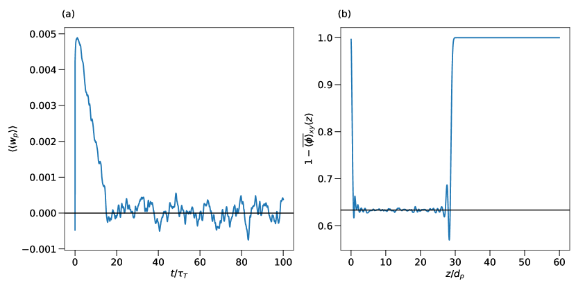
Figure 2: (a) Time series of the ensemble-average instantaneous vertical particle velocity $\langle\langle w_{p}\rangle\rangle$ showing how statistical equilibrium is reached at roughly $t=20\tau_{T}$, where $\tau_{T}=d_{p}/u_{0}$ is the particle turnover time and (b) vertical variation of time-average porosity $1-\langle\overline{\phi}\rangle_{xy}$ showing the effects of boundary conditions on the bottom and top of the fluidized bed for the case with $Re_{p}=40$.

In the simulations, the porosity decreases from unity at the inlet, remains relatively constant and then increases to unity at the top of the fluidized bed. Therefore, a spatially variable porosity is expected as compared to the homogeneous porosity in a fluidized bed away from boundaries. Including results from these two regions (top and bottom) would affect the accuracy and convergence of statistical quantities. To determine the region of homogeneous porosity, we define the instantaneous Eulerian volume fraction of the bed, $\phi(\boldsymbol{x},t)$ and compute horizontally-averaged (x- and y-directions) Eulerian volume fraction of the bed, $\langle\overline{\phi}\rangle_{xy}(z,t)$ as described in Appendix A. Figure 2(b) shows the time-averaged porosity $1-\langle\overline{\phi}\rangle_{xy}$ as a function of the vertical position $z/d_{p}$ for $Re_{p}=40$. The time-averaged porosity decreases to $0.63$ away from the inlet and then increases to $1$ at the top of the fluidized bed. To eliminate boundary effects, we define the modified spatial average for fluid variables as

$$\langle\{\cdot\}\rangle_{\beta}=\frac{1}{N_{\beta}}\sum_{i=1}^{N_{\beta}}\{\cdot\}_{ijk},$$ (7)

$$\langle\{\cdot\}\rangle_{z}=\frac{1}{N_{z}^{*}}\sum_{k=k_{s}}^{k_{e}}\{\cdot\}_{ijk},$$ (8)

$$\langle\{\cdot\}\rangle=\frac{1}{N_{x}N_{y}N_{z}^{*}}\sum_{i,j=1}^{N_{x},N_{y}}\sum_{k=k_{s}}^{k_{e}}\{\cdot\}_{ijk},$$ (9)

where $\beta=x$ or $y$ represents the horizontal directions, $k_{s}=z_{b}/h$ and $k_{e}=z_{t}/h$ are the nearest integer of the bottom and top of the fluidized-bed and $z_{b}$ and $z_{t}$ are the vertical position of the bottom and top of the homogeneous fluidized bed, respectively. The modified ensembled-average operator for particle variables is then defined as

$$\langle\{\cdot\}\rangle=\frac{1}{N_{p}^{*}}\sum_{i=1}^{N_{p}}\{\cdot\}_{i}\mathbf{1}_{z_{b}<z_{p}<z_{t}}(z_{p}),$$ (10)

where $N_{p}^{*}=\sum_{n=1}^{N_{p}}\mathbf{1}_{z_{b}<z_{p}<z_{t}}(z_{p})$ is the number of particles that are located within the homogeneous fluidized bed and

$$\mathbf{1}_{z_{b}<z_{p}<z_{t}}(z_{p})=\begin{cases}1&z_{b}<z_{p}<z_{t},\\ 0&\text{otherwise,}\end{cases}$$ (11)

is the indicator function that describes whether particles are located in the spatially homogeneous region of the fluidized bed.

The relationship between the upflow velocity and volume fraction of particles has been studied extensively (Yin & Koch, 2007; Richardson & Zaki, 1954; Garside & Al-Dibouni, 1977; Di Felice, 1995, 1999; Di Felice & Parodi, 1996; Willen & Prosperetti, 2019; Hamid et al., 2014; Zaidi et al., 2015; Nicolai et al., 1995) and is typically described by the power law relationship

$$u^{*}=\frac{u_{0}}{w_{ref}}=k(1-\langle\overline{\phi}\rangle)^{n}\,,$$ (12)

where $w_{ref}$ is the settling velocity of a single particle in the domain of interest, $k$ is a low volume fraction correction (Yin & Koch, 2007; Di Felice, 1995, 1999; Di Felice & Parodi, 1996) and $n$ is the expansion or power law exponent.The settling velocity of a single particle in an infinitely large domain, $w_{ref}$, is computed with (Yin & Koch, 2007)

$$Ar=\begin{cases}18Re_{t}[1+0.1315Re_{t}^{(0.82-0.05\log_{10}Re_{t})}],&0.01<\real_{t}<20\\ 18Re_{t}[1+0.1935Re_{t}^{0.6305}],&20<Re_{t}<260\end{cases}$$ (13)

where $Re_{t}=w_{ref}d_{p}/\nu$ and $Ar=(\rho_{p}/\rho_{f}-1)gd_{p}^{3}/\nu^{2}$ is the Archimedes number. In this work, $Ar=2.36\times 10^{4}$ giving $Re_{t}\approx 200$ which is within the range of equation 13. The error of equation 13 has been shown to range from 2% to 4% (Yin & Koch, 2007; Willen & Prosperetti, 2019). Fitting our results to equation 12 yields values of $k=0.72$ and $n=2.82$ that are consistent with published values (Yin & Koch, 2007; Willen & Prosperetti, 2019). In this paper we focus on the relationship between the porosity $1-\langle\overline{\phi}\rangle$ and $Re_{p}$ shown in figure 3, which also includes the power law fits and shows that the porosity increases with increasing $Re_{p}$.

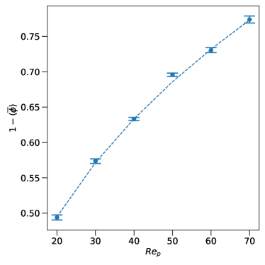
Figure 3: Porosity $1-\langle\overline{\phi}\rangle$ as a function of $Re_{p}$ for the simulated cases. The dashed lines were constructed based on fitting to the power law equation (12).

4.2 Kinematic wave speed

As discussed by many researchers (Sundaresan, 2003; Duru et al., 2002; Derksen & Sundaresan, 2007; Ham & Homsy, 1988), as $Re_{p}$ increases above $Re_{mf}=u_{mf}d_{p}/\nu$ where $Re_{mf}$ is the minimum fluidization Reynolds number, particles start to expand and upward-propagating waves can be observed. Below an intermediate $Re_{p}$, stable and neutral wave modes exist in which the amplitude of the waves decreases and remains approximately constant. For larger $Re_{p}$, unstable wave modes develop in which the wave amplitude grows with height, leading to large fluctuations in porosity. Zenit & Hunt (2000) investigated the time evolution of the ensemble- and time-averaged porosity $1-\langle\overline{\phi}\rangle$ and concluded that large-amplitude, low-frequency fluctuations dominated at low porosity (high volume fraction $\phi>0.3$) and small-amplitude, high-frequency fluctuations dominated at high porosity (low volume fraction $\phi<0.3$).

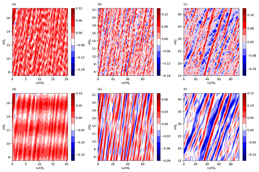
Figure 4: Volume fraction fluctuation $\langle\phi\rangle_{xy}^{\prime}$ as a function of time $u_{0}t/d_{p}$ and vertical position $z/d_{p}$ for the cases with $Re_{p}=20$, $40$ and $70$ from left to right. The second row represents the low wavenumber motions with wavenumber $k_{z}<k_{z,thresh}$.

Figure 4(a), (b) and (c) show two-dimensional $z-t$ plots of the volume fraction fluctuation $\langle\phi\rangle_{xy}^{\prime}=\langle\phi\rangle_{xy}-\langle\overline{\phi}\rangle_{xy}$. Waves can be identified visually but are difficult to quantify due to the presence of noise and superposition of waves with different modes. Researchers have reported that $\langle\phi\rangle_{xy}^{\prime}$ can be classified based on frequencies (Zenit & Hunt, 2000) or wavenumber (Willen et al., 2017). To separate low-wavenumber waves from the raw data, we modified the Fourier reconstruction method proposed by Willen et al. (2017) by defining low-wavenumber fluctuations for $k_{z}<k_{z,thresh}$, where $k_{z,thresh}=(z_{t}-z_{b})/2d_{p}$ is the threshold wavenumber. Since the behavior of small spatial-scale fluctuations ($k_{z}\geq k_{z,thresh}$) is an artifact of the spatial averaging, therefore, this study only focuses on the large-scale fluctuations ($k_{z}<k_{z,thresh}$) which allow interpretation of kinematic wave behavior. Figure 4(d), (e) and (f) show the low-wavenumber $\phi^{\prime}_{k_{z}<k_{z,thresh}}$. In general, upward-propagating waves are clearly observed with alternating regions of high and low porosity for $k_{z}<k_{z,thresh}$. For $Re_{p}=20$ (figure 4(d)), $\phi^{\prime}_{k_{z}<k_{z,thresh}}$ is a strong function of vertical position $z$ in which $\phi^{\prime}_{k_{z}<k_{z,thresh}}$ varies over a distance of $\sim 2d_{p}$ and depends weakly on time. For $Re_{p}>20$, wave motion is dependent both on time and vertical position.

The wave-like motions can be represented by a superposition of different waves with normalized wavenumber $k^{*}=kd_{p}$ and normalized frequency $\omega^{*}=\omega d_{p}/u_{0}$. Figure 5(a),(b) and (c) show the $\langle\phi\rangle_{xy}^{\prime}$ in spectral space as a function of $k^{*}$ and $\omega^{*}$. Overall, $\langle\phi\rangle_{xy}^{\prime}$ is dominated by low wavenumber waves with $k^{*}\approx 1$ and the dominant frequency $\omega^{*}$ decreases as $Re_{p}$ increases. At $Re_{p}=20$, regions of high $k^{*}-\omega^{*}$ can be observed even though the spectral density is relatively small. This illustrates that high-frequency wave modes are more significant at low $Re_{p}$ than high $Re_{p}$. As $Re_{p}$ increases, different modes collapse into a linear relationship. Figure 5(d),(e) and (f) show the $k^{*}-\omega^{*}$ spectra of $\phi^{\prime}_{k_{z}<k_{z,thresh}}$. For $\phi^{\prime}_{k_{z}<k_{z,thresh}}$, by eliminating high wavenumber modes, different modes of waves collapse into a line and a wave speed can be estimated from the kinematic relationship $\omega=ck$ using linear regression.

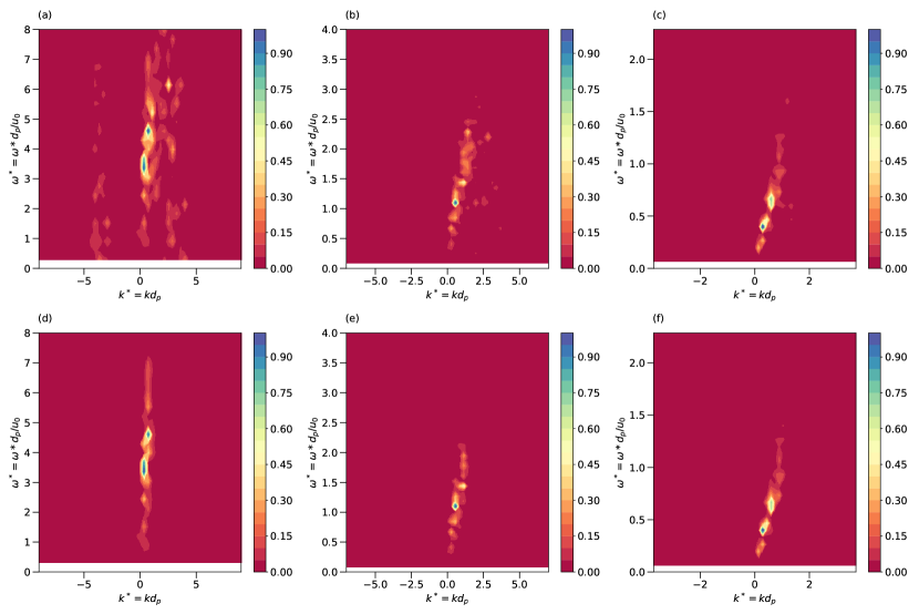
Figure 5: Energy spectra of volume fraction fluctuation $\langle\phi\rangle_{xy}^{\prime}$ as a function of normalized wavenumber $k^{*}$ and normalized frequency $\omega^{*}$ for the cases with $Re_{p}=20$, $40$ and $70$ from left to right and with $\phi^{\prime}$ and $\phi^{\prime}_{k_{z}<k_{z,thresh}}$ from top to bottom.

To demonstrate the existence of kinematic waves in the fluidized bed, we employ the model proposed by Wallis (2020) which relates volume fraction to wave speed with

$$c=kn\langle\overline{\phi}\rangle(1-\langle\overline{\phi}\rangle)^{n-1}w_{ref},$$ (14)

where $c$ is wave speed and other variables are defined in equation 12. To calculate the wave speed, we employ the two-dimensional autocorrelation approach as demonstrated by Yao et al. (2021). The autocorrelation of reconstructed volume fraction fluctuation $\phi^{\prime}_{k_{z}<k_{z,thresh}}$ is computed and wave speeds are calculated as the slope. As shown in figure 6, the calculated wave speeds are in agreement with the modeled values. The difference between the calculated wave speeds and modeled values are likely due to the dispersive effects which are not considered in equation 14 (Shajahan & Breugem, 2020; Wallis, 2020).

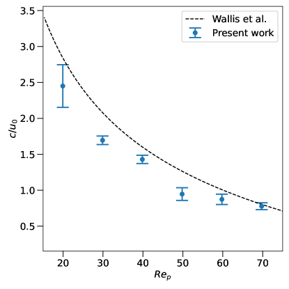
Figure 6: Wave speed based on the autocorrelation as a function of the particle Reynolds number $Re_{p}$.

4.3 Velocity fluctuations

In a fluidized bed, the ensemble-averaged vertical velocity $\langle\langle w\rangle\rangle=0$, indicating a balance between the submerged weight of the particles and the drag force. However, many researchers have reported that the velocity fluctuations can be as high as $10\%-170$% of the superficial velocity $u_{0}$ depending on the volume fractions (Willen & Prosperetti, 2019; Hamid et al., 2014; Zaidi et al., 2015; Nicolai et al., 1995). To understand the effect of $Re_{p}$ on the velocity fluctuations, we computed the root-mean-square velocity fluctuation

$$u_{rms,\alpha}=\overline{\sqrt{\langle u^{\prime}_{\alpha}u^{\prime}_{\alpha}\rangle}},$$ (15)

where $u^{\prime}_{\alpha}=u_{\alpha}-\langle\overline{u}\rangle_{\alpha}$ is the particle velocity fluctuation and $\alpha=x$, $y$ or $z$. Here, the overbar is the time average defined in equation (6) and the angular brackets $\langle\cdot\rangle$ imply an ensemble average over particles in the homogeneous region of the fluidized bed as defined in equation (10). Figure 7 shows $u_{rms,\alpha}$ normalized by $u_{0}$ as a function of $Re_{p}$. Both $u_{rms,x}$ and $u_{rms,z}$ increase initially and reach a maximum at $Re_{p}\approx 40$ and then decrease with increasing $Re_{p}$. Defining the anisotropy as $u_{rms,z}/u_{rms,x}$, for the range of $Re_{p}$ simulated, the anisotropy ranges between $1.7-1.8$. Similar trends were observed by Willen & Prosperetti (2019). While a maximum in velocity fluctuations is expected because they should be zero for both a single particle ($\phi\approx 0$) and a packed bed ($\phi\approx 0.6$), the physical mechanisms leading to a maximum at $Re_{p}\approx 40$ have not been reported in the literature.

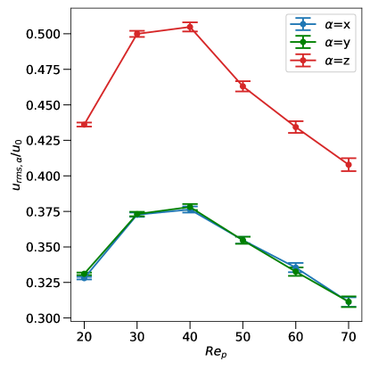
Figure 7: The root-mean-square velocity fluctuation normalized by the superficial velocity $u_{0}$ as a function of the particle Reynolds number $Re_{p}$.

In addition to particle velocity fluctuations, the fluid velocity fluctuations in the vicinity of the particles are also quantified. Many methods have been proposed to quantify the fluid velocity in the vicinity of the particles (Bagchi & Balachandar, 2003; Kidanemariam et al., 2013; Uhlmann & Doychev, 2014). In this study, we adopted the approach by Kidanemariam et al. (2013) where the fluid velocity in the vicinity of the particles is defined as the fluid in a spherical volume of diameter $2d_{p}$ where the center of the spherical volume coincides with the particle center. Figure 8 shows the fluid velocity fluctuations as a function of $Re_{p}$. Overall, the trends are very similar to the particle velocity fluctuations in figure 7. However, the magnitudes are smaller, indicating weaker fluid velocity fluctuations compared to the particles. It is likely that the inter-particle collisions leading to the particle velocity fluctuations occur over time scales that are too short for the fluid to respond, resulting in lower fluid velocity fluctuations.

Figure 8: The root-mean-square fluid velocity fluctuation in vicinity to particles normalized by the superficial velocity $u_{0}$ as a function of the particle Reynolds number $Re_{p}$.

4.4 Autocorrelation and pairwise distributions

To understand the processes governing the fluctuating particle motions, we compute the instantaneous velocity fluctuation autocorrelation for a given time lag $\tau$

$$R_{\alpha\alpha}(\tau)=\dfrac{\langle u^{\prime}_{\alpha}(t_{0})u^{\prime}_{\alpha}(t_{0}+\tau)\rangle}{\langle u^{\prime}_{\alpha}(t_{0})u^{\prime}_{\alpha}(t_{0})\rangle},$$ (16)

and the results are shown in figure 9. For all $Re_{p}$, the transverse velocity fluctuations ($R_{xx},R_{yy}$) for $1<u_{0}\tau/d_{p}<6$ indicate regimes of anti-correlation, the extent of which decreases with increasing Reynolds number. The axial velocity fluctuations $R_{zz}$ decorrelate monotonically to zero except for $Re_{p}=20$ and $30$ where a region of anti-correlation exists. In addition, the transverse velocity fluctuations decorrelate faster than the axial velocity fluctuations because of preferential excitation of random particle motions in the axial direction by the axial flow. Similar results have been reported by previous three-dimensional simulations and experimental results with different particle properties (Willen & Prosperetti, 2019; Esteghamatian et al., 2017; Nicolai et al., 1995).

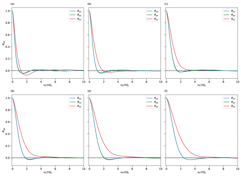
Figure 9: Transverse ($R_{xx},R_{yy}$) and axial ($R_{zz}$) velocity fluctuation autocorrelation as a function of the lag time $\tau$ (equation (16)) with different particle Reynolds numbers $Re_{p}$.(a) $Re_{p}=20$, (b) $30$, (c) $40$, (d) $50$, (e) $60$, (f) $70$.

The decorrelation time for the $\alpha$ component of the velocity fluctuations can be quantified by the true integral time scale

$$\mathcal{T}_{\alpha,\infty}=\int_{0}^{\infty}R_{\alpha\alpha}(\tau)\ \differential\tau\,.$$ (17)

However, in simulations where data is limited, the computed integral time scale is instead approximated with

$$\mathcal{T}_{\alpha,cal}=\int_{0}^{t_{f}}R_{\alpha\alpha}(\tau)\ \differential\tau\,,$$ (18)

where $t_{f}$ is the simulation time and $N_{\tau}=u_{0}t_{f}/d_{p}$ is the nondimensional time to calculate the computed integral timescale.

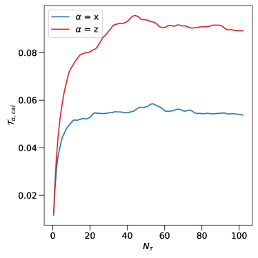
Figure 10: Computed integral timescale $\mathcal{T}_{\alpha,cal}$ as a function of $N_{\tau}$.

Figure 10 shows that the magnitude of $\mathcal{T}_{\alpha,cal}$ increases initially as a function of $N_{\tau}$ and fluctuates about a mean value due to the presence of wave-like autocorrelations. Similar wave-like autocorrelations were observed by Esteghamatian et al. (2017) and Nicolai et al. (1995). To quantify the error associated with the computed integral timescale, we computed the mean and standard deviation of $\mathcal{T}_{\alpha,cal}$ as

$$\mathbb{E}(\mathcal{T}_{\alpha,cal})=\dfrac{1}{N_{\tau}-N_{\tau,\text{thresh}}}\sum_{i=N_{\tau,\text{thresh}}}^{N_{\tau}}\mathcal{T}_{\alpha,cal}^{i},$$ (19)

$$\sigma(\mathcal{T}_{\alpha,cal})=\sqrt{\mathbb{E}(\mathcal{T}^{2}_{\alpha,cal})-\mathbb{E}(\mathcal{T}_{\alpha,cal})^{2}},$$ (20)

where $N_{\tau,\text{thresh}}$ is the minimum $N_{\tau}$ for $\mathcal{T}_{\alpha,cal}$ to reach equilibrium, and $\mathbb{E}(\mathcal{T}_{\alpha,cal})$ and $\sigma{(\mathcal{T}_{\alpha,cal})}$ are the mean and standard deviation of the calculated integral time scale, respectively.

Figure 11 shows the effect of $Re_{p}$ on $\mathbb{E}(\mathcal{T}_{\alpha,cal})$ and the ratio $\mathbb{E}(\mathcal{T}_{x,cal})/\mathbb{E}(\mathcal{T}_{z,cal})$, which is a measure of system anisotropy. Overall, $\mathbb{E}(\mathcal{T}_{z,cal})>\mathbb{E}(\mathcal{T}_{x,cal})$ for the range of $Re_{p}$ simulated, implying $\mathbb{E}(\mathcal{T}_{x,cal})/\mathbb{E}(\mathcal{T}_{z,cal})<1$. This is consistent with the fact that the axial velocity fluctuations take longer to decorrelate owing to the presence of the mean flow (Esteghamatian et al., 2017; Willen & Prosperetti, 2019; Nicolai et al., 1995). Interestingly, a minimum anisotropy (maximum of $\mathbb{E}(\mathcal{T}_{x,cal})/\mathbb{E}(\mathcal{T}_{z,cal})$) and maximum anisotropy (minimum of $\mathbb{E}(\mathcal{T}_{x,cal})/\mathbb{E}(\mathcal{T}_{z,cal})$) are observed at $Re_{p}=40$ and $50$, indicating most and least efficient momentum transfer, respectively. In addition, a sharp decrease in $\mathbb{E}(\mathcal{T}_{x,cal})/\mathbb{E}(\mathcal{T}_{z,cal})$ is observed as $Re_{p}$ increases from $40$ to $50$. This is due to the presence of competing mechanisms related to flow and particle physics, as discussed below.

We computed the normalized autocorrelation length scale, $\ell_{\alpha}^{*}=\ell_{\alpha}/d_{p}=u_{rms,\alpha}\mathbb{E}(\mathcal{T}_{\alpha,cal})/d_{p}$ which is a measure of the distance over which particle velocity fluctuations are still correlated, as shown in figure 12(a). When the particle velocity fluctuations are dominated by collisions when the porosity is low, the effects of velocity fluctuations do not propagate by more than the particle diameter, and thus $\ell_{\alpha}^{*}<1$. However, when $\ell_{\alpha}^{*}>1$ the particle velocity fluctuations are dominated by the effects of the mean flow on each particle since the effects of velocity fluctuations propagate further than a particle diameter. For all cases, both $\ell_{x}^{*}$ and $\ell_{z}^{*}$ are less than 1 indicating the particle velocity fluctuations are restricted by the relatively low porosity. Nicolai et al. (1995) reported $\ell_{z}^{*}>1$ for particle suspension in the Stokes regime, while Esteghamatian et al. (2017) reported $\ell_{z}^{*}<1$. We also computed $\ell_{x}/\ell_{z}$ which indicates anisotropy. As shown in figure 12(b), the anisotropy is maximized at $Re_{p}=40$ and decreases sharply between $Re_{p}=40$ and $Re_{p}=50$, indicating an increase in the anisotropy. This agrees with figure 11(b) where a sharp decrease is also observed from $Re_{p}=40$ to $Re_{p}=50$.

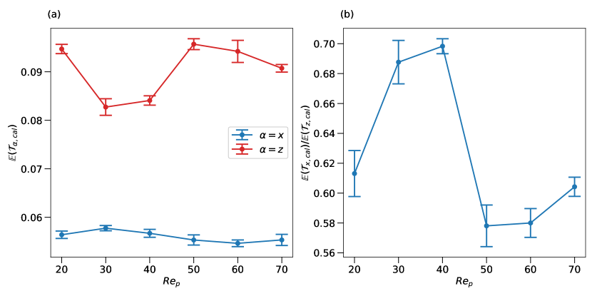
Figure 11: (a) The average integral time scales and (b) ratio of transverse integral timescale $\mathbb{E}(\mathcal{T}_{x,cal})$ to axial integral timescale $\mathbb{E}(\mathcal{T}_{z,cal})$ as a function of Reynolds number $Re_{p}$.

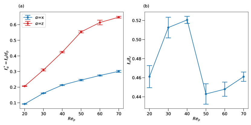
Figure 12: Effect of particle Reynolds number on (a) the autocorrelation distance $\ell_{\alpha}^{*}=\ell_{\alpha}/d_{p}$ and (b) ratio of transverse to axial autocorrelation distance $\ell_{x}/\ell_{z}$.

To highlight the different particle Reynolds number regimes leading to the anisotropy, we adapt the pairwise-probability density function from Yin & Koch (2008), which is given by

$$g(r,\theta)=g(\boldsymbol{r})=\frac{L_{x}L_{y}L_{b}}{d_{p}^{3}N_{p}^{2}}\left<\sum_{i=1}^{N_{p}}\sum_{j=1,j\neq i}^{N_{p}}\delta(\boldsymbol{r}-\boldsymbol{r}_{ij})\right>,$$ (21)

where $L_{b}=z_{t}-z_{b}$ is the height of the bed where the porosity is homogeneous, $\delta$ is defined as

$$\delta(\boldsymbol{r}-\boldsymbol{r}_{ij})=\begin{cases}1\ \ \ \ \boldsymbol{r}=\boldsymbol{r}_{ij},\\ 0\ \ \ \ \text{otherwise},\end{cases}$$ (22)

and $\boldsymbol{r}_{ij}=[r_{ij},\theta_{ij}]$ is the position vector between the center of particle $i$, $\boldsymbol{x}_{i}$, and particle $j$, $\boldsymbol{x}_{j}$. In cylindrical polar coordinates, $r_{ij}=\|\boldsymbol{x}_{i}-\boldsymbol{x}_{j}\|$ is the magnitude of $\boldsymbol{r}_{ij}$ and

$$\theta_{ij}=\begin{cases}\cos^{-1}[(|z_{i}-z_{j}|)/r_{ij}]&\text{if }z_{i}-z_{j}<0,\\ \sin^{-1}[(|z_{i}-z_{j}|)/r_{ij}]&\text{if }z_{i}-z_{j}\geq 0.\end{cases}$$ (23)

We also compute the pairwise-probability distribution function or radial distribution function as the angular average of $g(r,\theta)$ over three ranges: the entire range ($0\leq\theta\leq\pi/2$), an effective axial range ($0\leq\theta\leq\pi/12$) and an effective transverse range ($5\pi/12\leq\theta\leq\pi/2$). As shown in figure 13, the difference between the transverse and axial radial distribution functions is a measure of the particle arrangement preferences. The results indicate that particles do not have preferred arrangement over the $Re_{p}$ simulated, which is likely because the volume fractions we simulate are too large (Willen & Prosperetti, 2019; Yin & Koch, 2007). At $r/d=1$ and $r/d=2$, there is an obvious increase in the magnitude of the radial distribution function indicated by peaks in $g(r)$, an effect that decreases with increasing particle Reynolds number (see figure 14). This indicates that particles are more likely to appear at these two locations. Comparing with the three-dimensional simulations by Willen & Prosperetti (2019), in which the peak in the transverse $g(r)$ is slightly higher than the peak in the axial $g(r)$ (implying that a transverse arrangement of particle pairs is slightly favored over an axial arrangement), we found no difference between the transverse and axial arrangements. A possible explanation of this observation is due the higher $Re_{t}$ simulated in which the effect of collisions is more prominent. As a result, momentum is transferred more efficiently from the axial to transverse directions, inducing higher transverse velocity fluctuations and disrupting the arrangement of transverse particle pairs observed by Willen & Prosperetti (2019).

To further understand the effect of the particle Reynolds number, figure 14 shows the effect of $Re_{p}$ on $g(r/d_{p}=2)$. For the cases simulated, two regimes can be identified with regressions having correlation coefficients $R^{2}>0.99$. In general, the peak decreases with increasing Reynolds number, although the slope depends on two distinct flow regimes, which are referred to as Regime 1 ($Re_{p}<50$) and Regime 2 ($Re_{p}\geq 50$) in what follows.

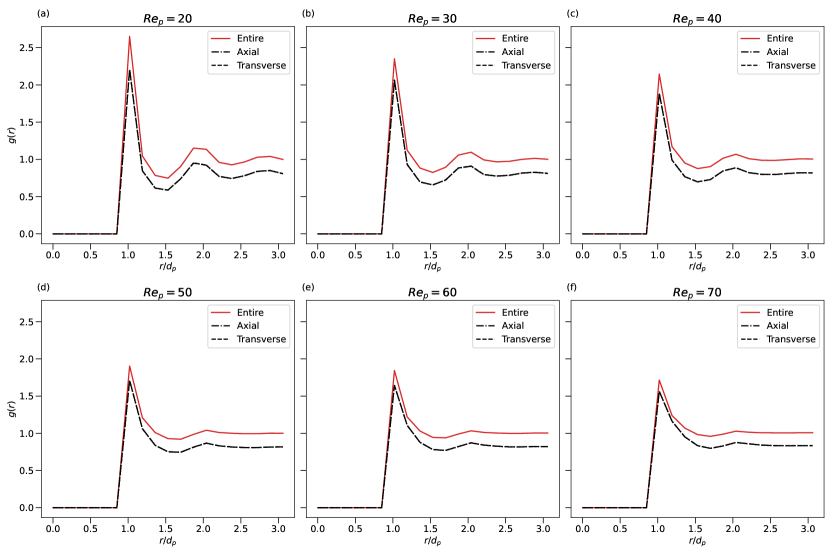
Figure 13: The pairwise distribution function, $g(r,\theta)$ (equation (21)) averaged over three ranges for the simulated cases with different $Re_{p}$.

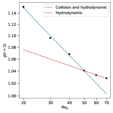
Figure 14: The radial distribution function at $r=2$, $g(r=2,\theta)$, averaged over $0\leq\theta\leq\pi/2$, for ranges of $Re_{p}$ simulated, with different regimes indicated by the lines obtained through linear regression.

4.5 Particle-particle and fluid-particle interactions

The mechanisms dictating the particle velocity fluctuations described in Section 4.4 can be explained through analysis of the magnitude of stresses related to the particle-particle and particle-fluid interactions. The role of particle-particle collisions is to transfer momentum from the axial direction to the transverse direction, resulting in a more isotropic system (Esteghamatian et al., 2017). To quantify the magnitude of the stress induced by collisions and flow, we computed the normal contact stress $\sigma_{col,\alpha}$, normal lubrication stress $\sigma_{lub,\alpha}$, and hydrodynamic stress due to the fluid $\sigma_{hydro,\alpha}$ as a function of the vertical position in the fluidized bed. The lubrication stress is considered separately from collision and hydrodynamic stresses since both fluid-particle and particle-particle interaction are involved. A detailed derivation of these stresses can be found in Appendix B. All stresses are normalized by $d_{p}^{2}/\rho_{f}\nu^{2}$ and denoted as $\widehat{\sigma}$.

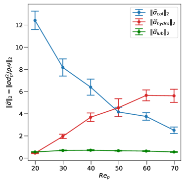
Figure 15: The computed normal contact stress, normal lubrication stress and hydrodynamic stress as a function of particle Reynolds number $Re_{p}$.

Overall, all the stresses fluctuate about a mean value away from the top and bottom boundaries of the fluidized bed. To quantify the effect of $Re_{p}$ on each component of the stress, we computed the vertical average of each stress first using the averaging operator defined in equation 7 and then computing the $\ell^{2}$ norm of the stress vector $\boldsymbol{\sigma}$ as $\norm{\boldsymbol{\sigma}}_{2}$. Figure 15 shows the magnitude of the normalized mean stresses as a function of $Re_{p}$. As $Re_{p}$ increases, the effect of $\norm{\boldsymbol{\sigma}_{col}}_{2}$ decreases while the effect of $\norm{\boldsymbol{\sigma}_{hydro}}_{2}$ increases. Both Zenit et al. (1997) and Derksen & Sundaresan (2007) have found $\norm{\boldsymbol{\sigma}_{col}}_{2}$ decreases with decreasing $\phi$ beyond a critical volume fraction. The effect of $\norm{\boldsymbol{\sigma}_{lub}}_{2}$ is negligible, which also agrees with Derksen & Sundaresan (2007) who showed that the lubrication stress is negligible even though the simulated porosity and particle properties are different.

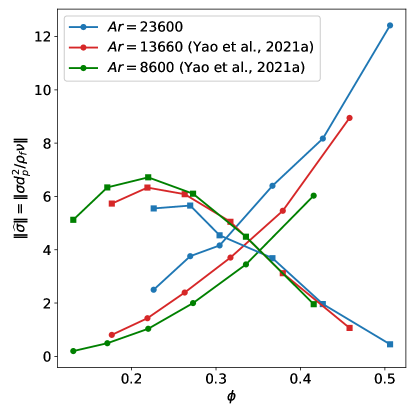
Figure 16: The computed normal contact stress (circle) and hydrodynamic stress (square) as a function of volume fraction $\phi$ for Archimedes numbers of 8600, 13660 and 23600.

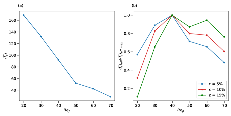
Figure 17: Time- and ensemble-averaged (a) collision frequency $\langle\overline{f_{c}}\rangle$ and (b) effective collision frequency $\langle\overline{f_{c}}\rangle_{\text{eff}}$ as a function of particle Reynolds number with different $\varepsilon$.

Comparing the magnitude of each stress (figure 15), at $Re_{p}=20$ where $\norm{\boldsymbol{\sigma}_{col}}_{2}>>\norm{\boldsymbol{\sigma}_{hydro}}_{2}$, collisions dominate over hydrodynamic effects and hydrodynamic effects are negligible. For $20<Re_{p}<40$, as $Re_{p}$ increases, hydrodynamic effects increase, $\norm{\boldsymbol{\sigma}_{col}}_{2}>\norm{\boldsymbol{\sigma}_{hydro}}_{2}$ still persists but the difference is decreasing. In this regime, collisions still dominate over hydrodynamic effects but the relative importance of hydrodynamic effects increases. This corresponds to Regime 1 in figure 14 where both collisions and hydrodynamics are important in inducing velocity fluctuations. For $Re_{p}>40$, $\norm{\boldsymbol{\sigma}_{hydro}}_{2}>\norm{\boldsymbol{\sigma}_{col}}_{2}$ indicates hydrodynamic effects dominating over collisions, corresponding to Regime 2 identified in figure 14. By comparing with results from Yao et al. (2021a) for simulations of fluidized beds with Archimedes number of 8600 and 13660 (figure 16), we observe that the critical volume fraction (inversely proportional to particle Reynolds number) decreases as the Archimedes number increases. However, future work is required to establish a relationship between the optimum particle Reynolds number and a wider range of Archimedes numbers.

The decreasing importance of the collisional stress with increasing $Re_{p}$ occurs because of a reduction in the collision frequency with increasing $Re_{p}$. We define a collision between two particles as occurring when the separation distance between the particle centers is less than the particle diameter $d_{p}$. If the number of times particle $i$ collides with another particle during a simulation time step $n$ is given by $N_{c,i}^{n}$, then the time- and ensembled-average collision frequency is given by

$$\langle\overline{f_{c}}\rangle=\frac{1}{N_{p}(t_{max}-t_{0})}\sum_{n=n_{0}}^{n_{max}}\sum_{i=1}^{N_{p}}N_{c,i}^{n}\,,$$ (24)

where $n_{0}=t_{0}/\Delta t$ and $n_{max}=t_{max}/\Delta t$. Since the porosity and in turn the spacing between particles increases with increasing $Re_{p}$ (figure 3), the likelihood of collisions should decrease with increasing $Re_{p}$, leading to the monotonically-decreasing dependence of $\langle\overline{f_{c}}\rangle$ on $Re_{p}$ as shown in figure 17(a). When the porosity is smaller, the likelihood of collision between particles is higher.

For the simulated cases, the collision frequency as defined in equation (24) is overestimated for small $Re_{p}$ because particles may interact without colliding and producing a measurable collisional stress. To restrict collisions to those with appreciable normal contact velocities, we define the collision Stokes number with impact velocity $u_{imp}$ as

$$St_{imp}=\dfrac{u_{imp}\rho_{p}d_{p}}{9\rho_{f}\nu},$$ (25)

where $u_{imp}$ is the normal component of the relative particle velocities contacting one another. The effective collision frequency, $\langle\overline{f_{c}}\rangle_{\text{eff}}$, is then computed by including collisions for which $St_{imp}>St_{thresh}$, where $St_{thresh}$ is a threshold Stokes number. The threshold Stokes number is determined by setting a minimum rebound velocity with an empirical function relating the restitution coefficient to the Stokes number. Defining the velocity of a particle before it is subjected to lubrication and contact forces as $w_{t,\infty}$, the restitution coefficient is given by

$$\varepsilon=\dfrac{u_{rebound}}{u_{t,\infty}}=\varepsilon_{\max}\exp(-\dfrac{30}{St_{\infty}}).$$ (26)

Here, $\varepsilon_{\max}\approx 0.91$ is the maximum restitution coefficient when $St_{\infty}\rightarrow\infty$ (Legendre et al., 2006), where

$$St_{\infty}=\dfrac{u_{t,\infty}d_{p}\rho_{p}}{9\rho_{f}\nu_{f}}.$$ (27)

In this work, since $u_{t,\infty}$ is difficult to quantify due to simultaneous collisions with the soft-sphere modeling approach, we rearrange equation 26 to relate $St_{imp}$ to $\varepsilon$ by using the dry restitution coefficient $e_{dry}=u_{rebound}/u_{imp}$ such that

$$St_{imp}=\dfrac{30\varepsilon}{e_{dry}(\log\varepsilon-\log\varepsilon_{\max})}=\dfrac{u_{imp}d_{p}\rho_{p}}{9\rho_{f}\nu_{f}}.$$ (28)

To understand the effect of different $\varepsilon$ on $St_{thresh}$, figure 24(b) shows the normalized effective collision frequency as a function of $Re_{p}$ for different $\varepsilon$. In general, as $\varepsilon$ increases, the effective collision frequency decreases and the maximum effective collision frequency shifts to higher $Re_{p}$. However, for the range of $\varepsilon$ tested, the maximum effective collision frequency occurs when $Re_{p}=40$, indicating that the maximum effective collision frequency is not very sensitive to $\varepsilon$. Furthermore, the maximum effective collision frequency coincides with the minimum anisotropy observed in figure 11 and figure 12, indicating a point in which momentum transfer from the axial to transverse directions is optimal.

5 Summary and conclusions

We studied the effects of the particle Reynolds number on the behavior of monodispersed spherical particles in PRS simulations of a three-dimensional, liquid-solid fluidized bed. The particle Reynolds number was varied by varying the flow rate suspending particles in the axial ($z$) direction. Analysis of various statistics provided insights into the observed particle motions. Boundary effects associated with the fluidized bed are identified and excluded in statistical calculations to improve accuracy. The wave modes are studied in both physical and spectral spaces to shed light on the source of the particle velocity fluctuations. By separating volume fraction fluctuations into low and high wavenumber components, wavelike behavior is clearly observed. For low particle Reynolds number ($Re_{p}=20$), waves with both low and high wavenumbers are strongly dependent on vertical position and weakly dependent on time. As particle Reynolds number increases, waves with low wavenumber depend strongly both on vertical positions and time while wave motions with high wavenumber are less apparent. Volume fraction fluctuations in spectral space further reveal that high-frequency wave modes are more significant at low particle Reynolds number. Low wavenumber modes can be estimated well with the kinematic wave relationship using linear regression while no discernible kinematic relationship can be observed for high wavenumber modes, indicating that the high wavenumber fluctuations are probably random. Analysis of the root-mean-square particle velocity fluctuations indicates a maximum at an intermediate particle Reynolds number ($Re_{p}=40$) in both the transverse and axial directions.

The decorrelation timescales in the axial and transverse directions reveal that momentum transfer from the axial to the transverse directions is most efficient at $Re_{p}=40$ and least efficient at $Re_{p}=50$. A sharp decrease in the efficiency of the momentum transfer is observed as $Re_{p}$ increases from 40 to 50, revealing a transition in the flow regime. Because the length scale over which particle motions decorrelate was less than $1d_{p}$ for all particle Reynolds numbers simulated. the transition is dominated by porosity effects. By analyzing the pairwise distribution function, we found that the probability that particle pairs are aligned at a distance of $2d_{p}$ decreases with increasing particle Reynolds number. The rate of this decrease revealed two distinct regimes that are consistent with the momentum transfer regimes discussed above.

To understand the mechanisms controlling the flow regimes and the sharp decrease in momentum transfer from the axial to transverse directions, we computed average collision and hydrodynamic stresses as a function of $Re_{p}$. The results indicate that the relative magnitude of collision to hydrodynamic effects controls the efficiency of inducing particle velocity fluctuations, momentum transfer and particle alignment. For $20<Re_{p}\leq 40$, collisions dominate over hydrodynamic effects but the relative importance of hydrodynamic effects increases, indicating a co-existence of mechanisms related to flow and collisions (Regime 1) that leads to the peak in particle velocity fluctuations and momentum transfer. As the particle Reynolds number increases ($Re_{p}>40$), hydrodynamic effects dominate over collision effects (Regime 2). Due to a lack of effective collisions, particle velocity fluctuations decrease and a sharp decrease in momentum transfer efficiency is observed. The lack of collisions arises from a decrease in the collision frequency with increasing $Re_{p}$. We found that it was important to quantify the collision frequency by an effective collision frequency based on collisions satisfying a threshold Stokes number. Defined this way, the effective collision frequency peaks at an $Re_{p}$ that coincides with that of the highest particle fluctuations and a sharp decrease in momentum transfer.

Our results imply biofilm detachment models in fluidized-bed reactors should focus on collision effects for $Re_{p}\leq Re_{p,\alpha}$, collision and hydrodynamic effects for $Re_{p,\alpha}<Re_{p}<Re_{p,\beta}$, and hydrodynamic effects for $Re_{p}\geq Re_{p,\beta}$ where $Re_{p,\alpha}\approx 40$ and $Re_{p,\beta}\approx 50$ for an Archimedes number of 23600. This study excludes the effect of adhesive force on biofilm and Archimedes number. Further work is required to quantify the effect of adhesive force on particle dynamics and establish a relationship between the optimum particle Reynolds number and Archimedes number. Furthermore, our results imply that mixing within liquid-solid fluidized bed reactors is likely to be optimized at an intermediate $Re_{p}$ at which particle velocity fluctuations are expected to be the strongest. Indeed, previous fluidized bed reactor studies with a large Archimedes number show that treatment performance is optimized at a similar intermediate $Re_{p}\approx 30-40$ (Jaafari et al., 2014). We anticipate that the results of this study will inform fluidized-bed reactor design and modeling for domestic and industrial wastewater treatment, enabling more reliable and energy-efficient operation.

Acknowledgments. This work used the Extreme Science and Engineering Discovery Environment (XSEDE), which is supported by National Science Foundation grant number ACI-1548562. Simulations were conducted with supercomputer resources under XSEDE Project CTS190063. The authors acknowledge the Texas Advanced Computing Center (TACC) at The University of Texas at Austin for providing HPC resources that have contributed to the research results reported within this paper. We thank Hyungoo Lee and Sivaramakrishnan Balachandar from the University of Florida for providing us with their IBM code. We also thank Edward Biegert, Bernhard Vowinckel, Thomas Köllner and Eckart Meiburg from the University of California, Santa Babara, for assistance with implementation of the collision models.

Funding. This work was funded by the California Energy Commission (CEC) under CEC project number EPC-16-017, the U.S. NSF Engineering Center for Reinventing of the Nation’s Urban Water Infrastructure (ReNUWIt) under Award No. 1028968, and Office of Naval Research Grant N00014-16-1-2256. This document was prepared as a result of work sponsored in part by the California Energy Commission. It does not necessarily represent the views of the Energy Commission, its employees, or the State of California. Neither the Commission, the State of California, nor the Commission’s employees, contractors, or subcontractors makes any warranty, express or implied, or assumes any legal liability for the information in this document; nor does any party represent that the use of this information will not infringe upon privately owned rights. This document has not been approved or disapproved by the Commission, nor has the Commission passed upon the accuracy of the information in this document.

Declaration of interests. The authors report no conflict of interest.

Author ORCID.
Yinuo Yao https://orcid.org/0000-0001-8328-6072
Craig Criddle https://orcid.org/0000-0002-2750-8547
Oliver Fringer https://orcid.org/0000-0003-3176-6925

Appendix A Instantaneous Eulerian volume fraction

In our simulations, the instantaneous Eulerian volume fraction $\phi(\boldsymbol{x},t)$ can be estimated using a second-order level-set approximation (Kempe & Fröhlich, 2012a). Defining the particle center as $\boldsymbol{x}_{p}$ and Eulerian grid as $\boldsymbol{x}_{ijk}$ where $i$, $j$ and $k$ represent each direction. The volume fraction of each grid cell is defined as

$$\phi(x_{i},y_{j},z_{k})=\dfrac{\sum_{l=1}^{8}-\psi_{m}\mathcal{H}(-\psi_{m})}{\sum_{l=1}^{8}\absolutevalue{\psi_{m}}},$$ (29)

where $l$ is an integer representing the corner of an Eulerian grid, $\psi$ is the level-set function for spheres that is defined as

$$\psi(\boldsymbol{x},\boldsymbol{x}_{p},r_{p})=\dfrac{\|\boldsymbol{x}-\boldsymbol{x}_{p}\|_{2}}{r_{p}}-1$$ (30)

and $\mathcal{H}(-\psi_{m})$ is the Heaviside function

$$\mathcal{H}(\alpha)=\begin{cases}0,&\alpha\leq 0,\\ 1,&\alpha>0.\end{cases}$$ (31)

To ensure the accuracy of level-approximation for $\phi(\boldsymbol{x},t)$, we use a grid spacing equivalent to the simulations where $h=d_{p}/25.6$.

Appendix B Determination of particle-related stresses

The governing equation of particle motion can be described as

$$m_{p}\derivative{\boldsymbol{u}_{p}}{t}=\boldsymbol{F}_{h,p}+\boldsymbol{F}_{col,p}+\boldsymbol{F}_{lub,p}-V_{p}(\rho_{p}-\rho_{f})\boldsymbol{g},$$ (32)

where $\boldsymbol{u}_{p}$ is the translational velocity of a particle, $\boldsymbol{F}_{h,p}$ is the drag force on the particle, $\boldsymbol{F}_{col,p}$ and $\boldsymbol{F}_{lub,p}$ are, respectively, the collision and normal lubrication force on particle $p$. Fluidization occurs when the weight of particle is balanced by the average drag force. Therefore, the drag force $F_{h,p}$ can be decomposed into two components such that

$$\boldsymbol{F}_{h,p}=\overline{\boldsymbol{F}_{h,p}}+\boldsymbol{F}_{h,p}^{\prime}=V_{p}(\rho_{p}-\rho_{f})\boldsymbol{g}+\boldsymbol{F}_{h,p}^{\prime},$$ (33)

where $\overline{\boldsymbol{F}_{h,p}}$ is the drag force that balances the weight of particle and $\boldsymbol{F}_{h,p}^{\prime}$ is the fluctuation force that results in acceleration. By substituting equation 33 into equation 32, the governing equation can be simplified as

$$m_{p}\derivative{\boldsymbol{u}_{p}}{t}=\boldsymbol{F}_{h,p}^{\prime}+\boldsymbol{F}_{col,p}+\boldsymbol{F}_{lub,p}.$$ (34)

In this study, the stresses due to $\boldsymbol{F}_{h,p}^{\prime}$, $\boldsymbol{F}_{lub,p}$ and $\boldsymbol{F}_{col,p}$ are defined as hydrodynamic, lubrication and collision stresses respectively. Since lubrication stress arises when two or more particles move closer to one another due to particle-particle interaction, therefore, lubrication stress is considered separately from the hydrodynamic stress in which the particle motion is only affected by the interaction between fluid and the particle.

The normal lubrication force and collision forces are only nonzero when the separation distance $\zeta_{n}$ between particle centers are less than $d_{p}+2h$ and $d_{p}$ respectively. As such, the governing equation of particle motion can be rewritten as

$$m_{p}\derivative{\boldsymbol{u}_{p}}{t}=\begin{cases}\boldsymbol{F}_{h,p}^{\prime},&\text{ for }\|\boldsymbol{x}_{p}-\boldsymbol{x}_{q}\|_{2}>d_{p}+2h,\\ \boldsymbol{F}_{h,p}^{\prime}+\boldsymbol{F}_{lub,p},&\text{ for }d_{p}<\|\boldsymbol{x}_{p}-\boldsymbol{x}_{q}\|_{2}\leq d_{p}+2h,\\ \boldsymbol{F}_{col,p},&\text{ for }\|\boldsymbol{x}_{p}-\boldsymbol{x}_{q}\|_{2}\leq d_{p},\end{cases}$$ (35)

where $x_{p}$ and $x_{q}$ are the particle center positions.

To determine the stresses as a function of vertical position in the domain, we first discretize the domain into slices with a vertical spacing of $d_{p}/2$. If we assume the acceleration of a particle at time step $n+1/2$ is given by

$$\boldsymbol{a}_{p}^{n+1/2}=\dfrac{\boldsymbol{u}_{p}^{n+1}-\boldsymbol{u}_{p}^{n}}{\Delta{t}}.$$ (36)

Then the total force $\boldsymbol{F}_{t,p}$ at time step $n+1/2$ is $m_{p}\boldsymbol{a}_{p}^{n+1/2}$. To demonstrate the validity of equation 35, we define an average error metric

$$\langle\boldsymbol{\varepsilon}_{f}\rangle=\dfrac{1}{N_{p}}\sum_{i=1}^{N_{p}}\dfrac{m_{p}\boldsymbol{a}_{i}^{n+1/2}}{\boldsymbol{F}^{n}_{i,rhs}}-1,$$ (37)

where $\boldsymbol{F}^{n}_{i,rhs}$ is the summation of all forces experienced by the particle $i$ at time $n$. As shown in table 1, the mean error associated with the approximation is less than 1% for all cases, demonstrating the validity of equation 35.

$Re_{p}$	20	30	40	50	60	70
$\langle\overline{\varepsilon_{f}}\rangle_{x}\times 10^{2}$	0.06 $\pm$ 2.17	0.14 $\pm$ 1.88	0.16 $\pm$ 1.76	0.21 $\pm$ 2.80	0.27 $\pm$ 1.97	0.26 $\pm$ 2.01
$\langle\overline{\varepsilon_{f}}\rangle_{y}\times 10^{2}$	0.06 $\pm$ 2.14	0.12 $\pm$ 1.91	0.17 $\pm$ 1.76	0.21 $\pm$ 2.83	0.26 $\pm$ 1.93	0.25 $\pm$ 1.93
$\langle\overline{\varepsilon_{f}}\rangle_{z}\times 10^{2}$	0.05 $\pm$ 2.17	0.12 $\pm$ 1.95	0.17 $\pm$ 1.78	0.24 $\pm$ 2.95	0.28 $\pm$ 2.02	0.26 $\pm$ 2.07

Table 1: Error $\boldsymbol{\varepsilon_{f}}$ associated with force balance in equation 35.

The hydrodynamic force at time step $n+1/2$ can be determined as

$$\boldsymbol{F}_{h,p}^{\prime}=\begin{cases}\boldsymbol{F}_{t,p},&\text{ for }\|\boldsymbol{x}_{p}-\boldsymbol{x}_{q}\|_{2}>d_{p}+2h,\\ \boldsymbol{F}_{t,p}-\boldsymbol{F}_{lub,p},&\text{ for }d_{p}<\|\boldsymbol{x}_{p}-\boldsymbol{x}_{q}\|_{2}\leq d_{p}+2h,\\ \end{cases}$$ (38)

and the hydrodynamic stress over particle surface area $(\sigma_{hydro,p})^{n+1/2}=\boldsymbol{F}_{h,p}^{\prime}/(\pi d_{p}^{2})$ can be calculated. The hydrodynamic stress for a particle bin $k$ can be calculated as

$$(\boldsymbol{\sigma}_{hydro})_{k}=\dfrac{1}{N}\sum_{n=1}^{N_{p}}\sum_{t=1}^{N_{t}}\dfrac{(|\boldsymbol{F}_{h}^{\prime}|)^{t}_{i}}{\pi d_{p}^{2}}\mathbf{1}_{z_{l}<z_{i}<z_{u}}(z_{i}),$$ (39)

where $N=\sum^{N_{t}N_{p}}\mathbf{1}_{z_{l}<z_{i}<z_{u}}(z_{i})$ is the number of samples in each bin, $z_{i}$ is the vertical position of particle $i$, $\boldsymbol{e}$ is vector of ones and $\mathbf{1}_{z_{l}<z_{i}<z_{u}}(z_{i})$ is the indicator function that is defined as

$$\mathbf{1}_{z_{l}<z_{p}<z_{u}}(z_{i})=\begin{cases}1&z_{l}<z_{p}<z_{u},\\ 0&\text{otherwise.}\end{cases}$$ (40)

In the simulations, the collision model is based on the Adaptive Collision Time Model (ACTM) proposed by Kempe & Fröhlich (2012a) and tangential collision models by Biegert et al. (2017). In ACTM, each collision is assumed to occur over $10\Delta{t}$ instead of $\Delta{t}$ in the soft-sphere collision model. At each time step, the normal contact force $\boldsymbol{F}_{col}$ is determined and the contributions of all collisions at a bin $k$ is determined with

$$(\boldsymbol{\sigma}_{col})_{k}=\dfrac{1}{N}\sum_{n=1}^{N_{p}}\sum_{t=1}^{N_{t}}\dfrac{(|\boldsymbol{F}_{con}|)^{t}_{i}}{\pi d_{p}^{2}}\mathbf{1}_{z_{l}<z_{i}<z_{u}}(z_{i}).$$ (41)

A similar procedure can be applied to the lubrication stress after assuming the lubrication forces are also stretched over several time steps. The contributions of all lubrication forces in a bin $k$ is determined with

$$(\boldsymbol{\sigma}_{lub})_{k}=\dfrac{1}{N}\sum_{n=1}^{N_{p}}\sum_{t=1}^{N_{t}}\dfrac{(|\boldsymbol{F}_{lub}|)^{t}_{i}}{\pi d_{p}^{2}}\mathbf{1}_{z_{l}<z_{i}<z_{u}}(z_{i}).$$ (42)

References

- Akiki et al. (2016) Akiki, G, Jackson, T L & Balachandar, S 2016 Force variation within arrays of monodisperse spherical particles. Phys. Rev. Fluids 1 (4), 044202.
- Akiki et al. (2017a) Akiki, G, Jackson, T L & Balachandar, S 2017a Pairwise interaction extended point-particle model for a random array of monodisperse spheres. J. Fluid Mech. 813, 882–928.
- Akiki et al. (2017b) Akiki, G, Moore, W C & Balachandar, S 2017b Pairwise-interaction extended point-particle model for particle-laden flows. J. Comput. Phys. 351, 329–357.
- Bagchi & Balachandar (2003) Bagchi, P & Balachandar, S 2003 Effect of turbulence on the drag and lift of a particle. Phys. Fluids 15 (11), 3496–3513.
- Biegert et al. (2017) Biegert, Edward, Vowinckel, Bernhard & Meiburg, Eckart 2017 A collision model for grain-resolving simulations of flows over dense, mobile, polydisperse granular sediment beds. J. Comput. Phys. 340, 105–127.
- Biegert (2018) Biegert, Edward Kristopher 2018 Eroding Uncertainty: Towards Understanding Flows Interacting with Mobile Sediment Beds Using Grain-Resolving Simulations. PhD thesis, UC Santa Barbara.
- Chang et al. (1991) Chang, H T, Rittmann, B E, Amar, D, Heim, R, Ehlinger, O & Lesty, Y 1991 Biofilm detachment mechanisms in a liquid-fluidized bed. Biotechnol. Bioeng. 38 (5), 499–506.
- Chow et al. (1998) Chow, Edmond, Cleary, Andrew J & Falgout, Robert D 1998 Design of the hypre Preconditioner Library. In SIAM Workshop on Object Oriented Methods for Inter-operable Scientific and Engineering Computing. SIAM.
- Costa et al. (2015) Costa, Pedro, Boersma, Bendiks Jan, Westerweel, Jerry & Breugem, Wim-Paul 2015 Collision model for fully resolved simulations of flows laden with finite-size particles. Phys. Rev. E Stat. Nonlin. Soft Matter Phys. 92 (5), 053012.
- Derksen & Sundaresan (2007) Derksen, J J & Sundaresan, S 2007 Direct numerical simulations of dense suspensions: wave instabilities in liquid-fluidized beds. J. Fluid Mech. 587, 303–336.
- Di Felice (1995) Di Felice, Renzo 1995 Hydrodynamics of liquid fluidisation. Chem. Eng. Sci. 50 (8), 1213–1245.
- Di Felice (1999) Di Felice, R 1999 The sedimentation velocity of dilute suspensions of nearly monosized spheres. Int. J. Multiphase Flow 25 (4), 559–574.
- Di Felice & Parodi (1996) Di Felice, Renzo & Parodi, Enrico 1996 Wall effects on the sedimentation velocity of suspensions in viscous flow. AIChE J. 42 (4), 927–931.
- Dieterich (1972) Dieterich, James H 1972 Time-dependent friction in rocks. J. Geophys. Res. 77 (20), 3690–3697.
- Duru et al. (2002) Duru, Paul, Nicolas, Maxime, Hinch, John & Guazzelli, Élisabeth 2002 Constitutive laws in liquid-fluidized beds. J. Fluid Mech. 452, 371–404.
- Esteghamatian et al. (2017) Esteghamatian, Amir, Hammouti, Abdelkader, Lance, Michel & Wachs, Anthony 2017 Particle resolved simulations of liquid/solid and gas/solid fluidized beds. Phys. Fluids 29 (3), 033302–1–033302–14.
- Falgout (2006) Falgout, R D 2006 An introduction to algebraic multigrid. Computing in Science Engineering 8 (6), 24–33.
- Finn & Apte (2013) Finn, Justin & Apte, Sourabh V 2013 Relative performance of body fitted and fictitious domain simulations of flow through fixed packed beds of spheres. Int. J. Multiphase Flow 56, 54–71.
- Foerster et al. (1994) Foerster, Samuel F, Louge, Michel Y, Chang, Hongder & Allia, Khédidja 1994 Measurements of the collision properties of small spheres. Phys. Fluids 6 (3), 1108–1115.
- Garside & Al-Dibouni (1977) Garside, John & Al-Dibouni, Maan R 1977 Velocity-Voidage Relationships for Fluidization and Sedimentation in Solid-Liquid Systems. Ind. Eng. Chem. Proc. Des. Dev. 16 (2), 206–214.
- Geldart (1973) Geldart, D 1973 Types of gas fluidization. Powder Technol. 7 (5), 285–292.
- Gjaltema et al. (1997) Gjaltema, A, Vinke, J L, van Loosdrecht, M C & Heijnen, J J 1997 Abrasion of suspended biofilm pellets in airlift reactors: importance of shape, structure, and particle concentrations. Biotechnol. Bioeng. 53 (1), 88–99.
- Ham & Homsy (1988) Ham, J M & Homsy, G M 1988 Hindered settling and hydrodynamic dispersion in quiescent sedimenting suspensions. Int. J. Multiphase Flow 14 (5), 533–546.
- Hamid et al. (2014) Hamid, Adnan, Molina, John J & Yamamoto, Ryoichi 2014 Direct numerical simulations of sedimenting spherical particles at non-zero Reynolds number. RSC Adv. 4 (96), 53681–53693.
- Jaafari et al. (2014) Jaafari, Jalil, Mesdaghinia, Alireza, Nabizadeh, Ramin, Hoseini, Mohammad, Kamani, Hossein & Mahvi, Amir Hossein 2014 Influence of upflow velocity on performance and biofilm characteristics of Anaerobic Fluidized Bed Reactor (AFBR) in treating high-strength wastewater. J Environ Health Sci Eng 12 (1), 139.
- Joseph & Hunt (2004) Joseph, G G & Hunt, M L 2004 Oblique particle–wall collisions in a liquid. J. Fluid Mech. 510, 71–93.
- Joseph et al. (2001) Joseph, G G, Zenit, R, Hunt, M L & Rosenwinkel, A M 2001 Particle–wall collisions in a viscous fluid. J. Fluid Mech. 433, 329–346.
- Kempe & Fröhlich (2012a) Kempe, Tobias & Fröhlich, Jochen 2012a An improved immersed boundary method with direct forcing for the simulation of particle laden flows. J. Comput. Phys. 231 (9), 3663–3684.
- Kempe & Fröhlich (2012b) Kempe, Tobias & Fröhlich, Jochen 2012b Collision modelling for the interface-resolved simulation of spherical particles in viscous fluids. J. Fluid Mech. 709, 445–489.
- Kidanemariam et al. (2013) Kidanemariam, Aman G, Chan-Braun, Clemens, Doychev, Todor & Uhlmann, Markus 2013 Direct numerical simulation of horizontal open channel flow with finite-size, heavy particles at low solid volume fraction. New J. Phys. 15 (2), 025031.
- Kriebitzsch et al. (2013) Kriebitzsch, S H L, van der Hoef, M A & Kuipers, J A M 2013 Fully resolved simulation of a gas-fluidized bed: A critical test of DEM models. Chem. Eng. Sci. 91, 1–4.
- Lee & Balachandar (2010) Lee, Hyungoo & Balachandar, S 2010 Drag and lift forces on a spherical particle moving on a wall in a shear flow at finite Re. J. Fluid Mech. 657, 89–125.
- Lee et al. (2011) Lee, Hyungoo, Ha, Man Yeong & Balachandar, S 2011 Rolling/sliding of a particle on a flat wall in a linear shear flow at finite Re. Int. J. Multiphase Flow 37 (2), 108–124.
- Legendre et al. (2006) Legendre, Dominique, Zenit, Roberto, Daniel, Claude & Guiraud, Pascal 2006 A note on the modelling of the bouncing of spherical drops or solid spheres on a wall in viscous fluid. Chem. Eng. Sci. 61 (11), 3543–3549.
- Lu et al. (2020) Lu, Jiangtao, Peters, Elias A J F & Kuipers, Johannes A M 2020 Direct numerical simulation of mass transfer in bidisperse arrays of spheres. AIChE J. 66 (1).
- Nicolai et al. (1995) Nicolai, H, Herzhaft, B, Hinch, E J, Oger, L & Guazzelli, E 1995 Particle velocity fluctuations and hydrodynamic self‐diffusion of sedimenting non‐Brownian spheres. Phys. Fluids 7 (1), 12–23.
- Nicolella et al. (1997) Nicolella, Cristiano, Chiarle, Stefania, Di Felice, Renzo & Rovatti, Mauro 1997 Mechanisms of biofilm detachment in fluidized bed reactors. Water Sci. Technol. 36 (1), 229–235.
- Nicolella et al. (1996) Nicolella, C, Di Felice, R & Rovatti, M 1996 An experimental model of biofilm detachment in liquid fluidized bed biological reactors. Biotechnol. Bioeng. 51 (6), 713–719.
- Ozel et al. (2017) Ozel, A, Brändle de Motta, J C, Abbas, M, Fede, P, Masbernat, O, Vincent, S, Estivalezes, J-L & Simonin, O 2017 Particle resolved direct numerical simulation of a liquid–solid fluidized bed: Comparison with experimental data. Int. J. Multiphase Flow 89, 228–240.
- Pan et al. (2016) Pan, Hui, Chen, Xi-Zhong, Liang, Xiao-Fei, Zhu, Li-Tao & Luo, Zheng-Hong 2016 CFD simulations of gas–liquid–solid flow in fluidized bed reactors — A review. Powder Technol. 299, 235–258.
- Peskin (1977) Peskin, Charles S 1977 Numerical analysis of blood flow in the heart. J. Comput. Phys. 25 (3), 220–252.
- Rai & Moin (1991) Rai, Man & Moin, Parviz 1991 Direct simulations of turbulent flow using finite-difference schemes. J. Comput. Phys. 96 (1), 15–53.
- Richardson & Zaki (1954) Richardson, J F & Zaki, W N 1954 Sedimentation and Fluidisation: Part I. Trans. Inst. Chem. Eng. 32, 35–53.
- Rittmann & McCarty (2018) Rittmann, Bruce E & McCarty, Perry L 2018 Environmental Biotechnology: Principles and Applications. Columbus, OH: McGraw-Hill Education.
- Roma et al. (1999) Roma, Alexandre M, Peskin, Charles S & Berger, Marsha J 1999 An Adaptive Version of the Immersed Boundary Method. J. Comput. Phys. 153 (2), 509–534.
- Shajahan & Breugem (2020) Shajahan, Tariq & Breugem, Wim-Paul 2020 Influence of Concentration on Sedimentation of a Dense Suspension in a Viscous Fluid. Flow Turbul. Combust. 105 (2), 537–554.
- Shin et al. (2012) Shin, Chungheon, Bae, Jaeho & McCarty, Perry L 2012 Lower operational limits to volatile fatty acid degradation with dilute wastewaters in an anaerobic fluidized bed reactor. Bioresour. Technol. 109, 13–20.
- Shin et al. (2011) Shin, Chungheon, Lee, Eunyoung, McCarty, Perry L & Bae, Jaeho 2011 Effects of influent DO/COD ratio on the performance of an anaerobic fluidized bed reactor fed low-strength synthetic wastewater. Bioresour. Technol. 102 (21), 9860–9865.
- Shin et al. (2014) Shin, Chungheon, McCarty, Perry L, Kim, Jeonghwan & Bae, Jaeho 2014 Pilot-scale temperate-climate treatment of domestic wastewater with a staged anaerobic fluidized membrane bioreactor (SAF-MBR). Bioresour. Technol. 159, 95–103.
- Sundaresan (2003) Sundaresan, Sankaran 2003 Instabilities in fluidized beds. Annu. Rev. Fluid Mech. 35 (1), 63–88.
- Tang et al. (2015) Tang, Y, Peters, E A J F, Kuipers, J A M, Kriebitzsch, S H L & van der Hoef, M A 2015 A new drag correlation from fully resolved simulations of flow past monodisperse static arrays of spheres. AIChE J. 61 (2), 688–698.
- Tenneti et al. (2011) Tenneti, S, Garg, R & Subramaniam, S 2011 Drag law for monodisperse gas–solid systems using particle-resolved direct numerical simulation of flow past fixed assemblies of spheres. Int. J. Multiphase Flow 37 (9), 1072–1092.
- Uhlmann (2005) Uhlmann, Markus 2005 An immersed boundary method with direct forcing for the simulation of particulate flows. J. Comput. Phys. 209 (2), 448–476.
- Uhlmann & Doychev (2014) Uhlmann, Markus & Doychev, Todor 2014 Sedimentation of a dilute suspension of rigid spheres at intermediate Galileo numbers: the effect of clustering upon the particle motion. J. Fluid Mech. 752, 310–348.
- Verma et al. (2015) Verma, Vikrant, Padding, Johan T, Deen, Niels G & Hans Kuipers, J A M 2015 Effect of bed size on hydrodynamics in 3-D gas-solid fluidized beds. AIChE J. 61 (5), 1492–1506.
- Verma et al. (2014) Verma, Vikrant, Padding, Johan T, Deen, Niels G & Kuipers, J A M (hans) 2014 Numerical Investigation on the Effect of Pressure on Fluidization in a 3D Fluidized Bed. Ind. Eng. Chem. Res. 53 (44), 17487–17498.
- Wallis (2020) Wallis, Graham B 2020 One-Dimensional Two-Phase Flow. Courier Dover Publications.
- Wang et al. (2008) Wang, Zeli, Fan, Jianren & Luo, Kun 2008 Combined multi-direct forcing and immersed boundary method for simulating flows with moving particles. Int. J. Multiphase Flow 34 (3), 283–302.
- Willen & Prosperetti (2019) Willen, Daniel P & Prosperetti, Andrea 2019 Resolved simulations of sedimenting suspensions of spheres. Phys. Rev. Fluids 4 (1), 014304.
- Willen et al. (2017) Willen, Daniel P, Sierakowski, Adam J, Zhou, Gedi & Prosperetti, Andrea 2017 Continuity waves in resolved-particle simulations of fluidized beds. Phys. Rev. Fluids 2 (11), 114305.
- Yang et al. (2017) Yang, Min, Yu, Dawei, Liu, Mengmeng, Zheng, Libing, Zheng, Xiang, Wei, Yuansong, Wang, Fang & Fan, Yaobo 2017 Optimization of MBR hydrodynamics for cake layer fouling control through CFD simulation and RSM design. Bioresour. Technol. 227, 102–111.
- Yao et al. (2021a) Yao, Yinuo, Criddle, Craig S & Fringer, Oliver B 2021a Comparison of the properties of segregated layers in a bidispersed fluidized bed to those of a monodispersed fluidized bed. Phys. Rev. Fluids 6, 084306.
- Yao et al. (2021b) Yao, Yinuo, Criddle, Craig S & Fringer, Oliver B 2021b The effects of particle clustering on hindered settling in high-concentration particle suspensions. J. Fluid Mech. 920, A40.
- Yin & Koch (2007) Yin, Xiaolong & Koch, Donald L 2007 Hindered settling velocity and microstructure in suspensions of solid spheres with moderate Reynolds numbers. Phys. Fluids 19 (9), 093302.
- Yin & Koch (2008) Yin, Xiaolong & Koch, Donald L 2008 Lattice-Boltzmann simulation of finite Reynolds number buoyancy-driven bubbly flows in periodic and wall-bounded domains. Phys. Fluids 20 (10), 103304.
- Yu & Xu (2003) Yu, A?b & Xu, B?h 2003 Particle-scale modelling of gas-solid flow in fluidisation. J. Chem. Technol. Biotechnol. 78 (2-3), 111–121.
- Zaidi et al. (2015) Zaidi, Ali Abbas, Tsuji, Takuya & Tanaka, Toshitsugu 2015 Hindered Settling Velocity & Structure Formation during Particle Settling by Direct Numerical Simulation. Procedia Eng. 102, 1656–1666.
- Zang et al. (1994) Zang, Yan, Street, Robert L & Koseff, Jeffrey R 1994 A Non-staggered Grid, Fractional Step Method for Time-Dependent Incompressible Navier-Stokes Equations in Curvilinear Coordinates. J. Comput. Phys. 114 (1), 18–33.
- Zenit & Hunt (2000) Zenit, Roberto & Hunt, Melany L 2000 Solid fraction fluctuations in solid–liquid flows. Int. J. Multiphase Flow 26 (5), 763–781.
- Zenit et al. (1997) Zenit, R, Hunt, M L & Brennen, C E 1997 Collisional particle pressure measurements in solid–liquid flows. J. Fluid Mech. 353, 261–283.
- Zhang & Prosperetti (2005) Zhang, Z & Prosperetti, A 2005 A second-order method for three-dimensional particle simulation. J. Comput. Phys. 210 (1), 292–324.