Differentially Private Federated Learning via Inexact ADMM

Minseok Ryu
Mathematics and Computer Science Division
Argonne National Laboratory
Lemont, IL 60439
mryu@anl.gov
&Kibaek Kim
Mathematics and Computer Science Division
Argonne National Laboratory
Lemont, IL 60439
kimk@anl.gov
Abstract

Differential privacy (DP) techniques can be applied to the federated learning model to protect data privacy against inference attacks to communication among the learning agents. The DP techniques, however, hinder achieving a greater learning performance while ensuring strong data privacy. In this paper we develop a DP inexact alternating direction method of multipliers algorithm that solves a sequence of subproblems with the objective perturbation by random noises generated from a Laplace distribution. We show that our algorithm provides ϵ¯¯italic-ϵ\bar{\epsilon}-DP for every iteration, where ϵ¯¯italic-ϵ\bar{\epsilon} is a privacy parameter controlled by a user. Using MNIST and FEMNIST datasets for the image classification, we demonstrate that our algorithm reduces the testing error by at most 22%percent2222\% compared with the existing DP algorithm, while achieving the same level of data privacy. The numerical experiment also shows that our algorithm converges faster than the existing algorithm.

1 Introduction

In this work we propose a privacy-preserving algorithm for solving a federated learning (FL) model [16], namely, a machine learning (ML) model that aims to learn global model parameters without collecting locally stored data into a central server. The proposed algorithm is based on an inexact alternating direction method of multipliers (IADMM) that solves a sequence of subproblems whose objective functions are perturbed by injecting some random noises for ensuring differential privacy (DP) on the distributed data. We show that the proposed algorithm provides more accurate solutions compared with the state-of-the-art DP algorithm [10] while both algorithms provide the same level of data privacy. As a result, the proposed algorithm can mitigate a trade-off between data privacy and solution accuracy (i.e., learning performance in the context of ML), which is one of the main challenges in developing DP algorithms as described in [7].

Developing highly accurate privacy-preserving algorithms can enhance the practical uses of FL in applications with sensitive data (e.g., electronic health records [26] and mobile device data [23]) because a greater learning performance can be achieved while preserving privacy on the sensitive data exposed to be leaked during a training process. Because of the importance of FL, incorporating privacy-preserving techniques into optimization algorithms for solving the FL models has been studied extensively.

Related Work. The empirical risk minimization (ERM) model used for learning parameters in supervised ML is often vulnerable to adversarial attacks [22], a situation that motivates the application of privacy-preserving techniques (e.g., DP [6] and homomorphic encryption [13]) to protect data. Among these techniques, DP has been widely used in the ML community and is especially useful for protecting data against inference attacks [27].

Formally, DP is a privacy-preserving technique that randomizes the output of an algorithm such that any single data point cannot be inferred by an adversary that can reverse-engineer the randomized output. Depending on where to inject noises to randomize the output, DP can be categorized by input [9, 14], output [6, 5], and objective [5, 15] perturbation methods. Compared with input perturbation, which directly perturbs input data by adding random noises, output perturbation and objective perturbation methods provide a randomized output of an optimization problem by injecting random noises into its true output and objective function, respectively. In [5], the authors propose a differentially private ERM that utilizes the output and objective perturbation methods to ensure DP on data. Also, Abadi et al. [1] apply the output perturbation to stochastic gradient descent (SGD) in order to ensure DP on data for every iteration of the algorithm. The privacy-preserving technique in our work is the objective perturbation method: we randomize the output of the trust-region subproblem by perturbing its objective function with some random noises. For details of differentially private ML, we refer readers to [25, 15, 11].

Within the context of FL, various distributed optimization algorithms have been developed for solving the distributed ERM model. For example, FedAvg in [23] is an algorithm that combines SGD for each agent with a central server that performs model averaging. Another example is FedProx in [21] that is constructed by replacing the local SGD in FedAvg with an optimization problem with an additional proximal function. These algorithms do not guarantee data privacy during a training process, however, preventing their practical uses. Readers interested in details of FL should see [12, 18, 20]; for details about FL without the central server, see [19, 8].

In order to preserve privacy on data used for the FL model, various DP algorithms have been proposed in the literature, where the output and objective perturbations are incorporated for ensuring DP (see [2, 29, 24, 30, 10]). For example, the intermediate model parameters and/or gradients computed for every iteration of the FedAvg-type and FedProx-type algorithms are perturbed for guaranteeing DP as in [24] and [29], respectively, which can be seen as the output perturbation. Also, in [30], the primal and dual variables computed for every iteration of the ADMM algorithm are perturbed, which can be seen as the output and objective perturbations, respectively. Zhang and Zhu [30] compare the two perturbation methods, as [5] did under the general ML setting, and show that the objective perturbation can provide more accurate solutions compared with the output perturbation. The use of the objective perturbation is somewhat limited, however, because it requires the objective function to be twice differentiable and strongly convex whereas the twice differentiability restriction can be relaxed to the differentiability for the output perturbation. In [10], the authors incorporate the output perturbation into IADMM that utilizes the first-order approximation with a proximal function. Introducing the first-order approximation in ADMM enforces smoothness of the objective function, hence satisfying the aforementioned differentiability assumption for ensuring DP. Also, the authors show that the algorithm has 𝒪(1/T)𝒪1𝑇\mathcal{O}(1/\sqrt{T}) rate of convergence in expectation, where T𝑇T is the number of iterations. Moreover, their numerical experiments demonstrate that the algorithm outperforms DP-ADMM in [30] and DP-SGD in [1].

Contributions. In this paper, as compared with the DP-IADMM algorithm in [10], we incorporate the objective perturbation into IADMM that utilizes the first-order approximation. Our main contributions are summarized as follows:

  • Proof that the our new IADMM algorithm provides DP on data

  • Numerical demonstration that our DP algorithm provides more accurate solutions compared with the existing DP algorithm [10]

Organization and Notation. The remainder of the paper is organized as follows. In Section 2 we describe an FL model using a distributed ERM and present the existing inexact ADMM algorithm for solving the FL model. In Section 3 we propose a new DP inexact ADMM algorithm for solving the FL model that ensures DP on data and converges to an optimal solution with the sublinear convergence rate. In Section 4 we describe numerical experiments to demonstrate the outperformance of the proposed algorithm.

We denote by \mathbb{N} a set of natural numbers. For A𝐴A\in\mathbb{N}, we define [A]:={1,,A}assigndelimited-[]𝐴1𝐴[A]:=\{1,\ldots,A\} and denote by 𝕀Asubscript𝕀𝐴\mathbb{I}_{A} a A×A𝐴𝐴A\times A identity matrix. We use ,\langle\cdot,\cdot\rangle and \|\cdot\| to denote the scalar product and the Euclidean norm, respectively.

2 Federated Learning Model

Distributed ERM. Consider a set [P]delimited-[]𝑃[P] of agents connected to a central server. Each agent p[P]𝑝delimited-[]𝑃p\in[P] has a training dataset 𝒟p:={xpi,ypi}i=1Ipassignsubscript𝒟𝑝superscriptsubscriptsubscript𝑥𝑝𝑖subscript𝑦𝑝𝑖𝑖1subscript𝐼𝑝\mathcal{D}_{p}:=\{x_{pi},y_{pi}\}_{i=1}^{I_{p}}, where Ipsubscript𝐼𝑝I_{p} is the number of data samples, xpiJsubscript𝑥𝑝𝑖superscript𝐽x_{pi}\in\mathbb{R}^{J} is a J𝐽J-dimensional data feature, and ypiKsubscript𝑦𝑝𝑖superscript𝐾y_{pi}\in\mathbb{R}^{K} is a K𝐾K-dimensional data label. We consider a distributed ERM problem given by

minw𝒲subscript𝑤𝒲\displaystyle\min_{w\in\mathcal{W}}\ p=1P{1Ii=1Ip(w;xpi,ypi)+βPr(w)},superscriptsubscript𝑝1𝑃1𝐼superscriptsubscript𝑖1subscript𝐼𝑝𝑤subscript𝑥𝑝𝑖subscript𝑦𝑝𝑖𝛽𝑃𝑟𝑤\displaystyle\textstyle\sum_{p=1}^{P}\Big{\{}\frac{1}{I}\sum_{i=1}^{I_{p}}\ell(w;x_{pi},y_{pi})+\frac{\beta}{P}r(w)\Big{\}}, (1)

where wJ×K𝑤superscript𝐽𝐾w\in\mathbb{R}^{J\times K} is a global model parameter vector, 𝒲𝒲\mathcal{W} is a compact convex set, ()\ell(\cdot) is a convex loss function, r()𝑟r(\cdot) is a convex regularizer function, β>0𝛽0\beta>0 is a regularizer parameter, and I:=p=1PIpassign𝐼superscriptsubscript𝑝1𝑃subscript𝐼𝑝I:=\sum_{p=1}^{P}I_{p}. Since (1) is a convex optimization problem, it can be expressed by an equivalent Lagrangian dual problem. More specifically, we first rewrite (1) as

minw,z1,,zP𝒲subscript𝑤subscript𝑧1subscript𝑧𝑃𝒲\displaystyle\min_{w,z_{1},\ldots,z_{P}\in\mathcal{W}}\ p=1Pfp(zp;𝒟p)superscriptsubscript𝑝1𝑃subscript𝑓𝑝subscript𝑧𝑝subscript𝒟𝑝\displaystyle\textstyle\sum_{p=1}^{P}f_{p}(z_{p};\mathcal{D}_{p}) (2a)
s.t. wjk=zpjk,p[P],j[J],k[K],formulae-sequencesubscript𝑤𝑗𝑘subscript𝑧𝑝𝑗𝑘formulae-sequencefor-all𝑝delimited-[]𝑃formulae-sequencefor-all𝑗delimited-[]𝐽for-all𝑘delimited-[]𝐾\displaystyle w_{jk}=z_{pjk},\ \forall p\in[P],\forall j\in[J],\forall k\in[K], (2b)
where zpJ×Ksubscript𝑧𝑝superscript𝐽𝐾z_{p}\in\mathbb{R}^{J\times K} is a local parameter vector defined for every agent p[P]𝑝delimited-[]𝑃p\in[P] and
fp(zp;𝒟p):=1Ii=1Ip(zp;xpi,ypi)+βPr(zp).assignsubscript𝑓𝑝subscript𝑧𝑝subscript𝒟𝑝1𝐼superscriptsubscript𝑖1subscript𝐼𝑝subscript𝑧𝑝subscript𝑥𝑝𝑖subscript𝑦𝑝𝑖𝛽𝑃𝑟subscript𝑧𝑝\displaystyle f_{p}(z_{p};\mathcal{D}_{p}):=\textstyle\frac{1}{I}\sum_{i=1}^{I_{p}}\ell(z_{p};x_{pi},y_{pi})+\frac{\beta}{P}r(z_{p}). (2c)

By introducing dual variables λpJ×Ksubscript𝜆𝑝superscript𝐽𝐾\lambda_{p}\in\mathbb{R}^{J\times K} associated with constraints (2b), the Lagrangian dual problem is given by

maxλ1,,λPminw,z1,,zP𝒲p=1Pfp(zp;𝒟p)+λp,wzp.subscriptsubscript𝜆1subscript𝜆𝑃subscript𝑤subscript𝑧1subscript𝑧𝑃𝒲superscriptsubscript𝑝1𝑃subscript𝑓𝑝subscript𝑧𝑝subscript𝒟𝑝subscript𝜆𝑝𝑤subscript𝑧𝑝\displaystyle\max_{\lambda_{1},\ldots,\lambda_{P}}\ \min_{w,z_{1},\ldots,z_{P}\in\mathcal{W}}\ \ \textstyle\sum_{p=1}^{P}f_{p}(z_{p};\mathcal{D}_{p})+\langle\lambda_{p},w-z_{p}\rangle. (3)

Since (2) is a convex optimization problem, solving (3) provides an optimal solution to (2).

Inexact ADMM. ADMM is an iterative optimization algorithm that can find an optimal solution of (3) in the augmented Lagrangian form. More specifically, for every iteration t[T]𝑡delimited-[]𝑇t\in[T], it updates (wt,zt,λt)(wt+1,zt+1,λt+1)superscript𝑤𝑡superscript𝑧𝑡superscript𝜆𝑡superscript𝑤𝑡1superscript𝑧𝑡1superscript𝜆𝑡1(w^{t},z^{t},\lambda^{t})\rightarrow(w^{t+1},z^{t+1},\lambda^{t+1}) by solving a sequence of the following subproblems:

wt+1argminwp=1Pλpt,w+ρt2wzpt2,superscript𝑤𝑡1subscriptargmin𝑤superscriptsubscript𝑝1𝑃subscriptsuperscript𝜆𝑡𝑝𝑤superscript𝜌𝑡2superscriptnorm𝑤subscriptsuperscript𝑧𝑡𝑝2\displaystyle w^{t+1}\leftarrow\operatorname*{arg\,min}_{w}\ \textstyle\sum_{p=1}^{P}\langle\lambda^{t}_{p},w\rangle+\frac{\rho^{t}}{2}\|w-z^{t}_{p}\|^{2}, (4a)
zpt+1argminzp𝒲fp(zp;𝒟p)λpt,zp+ρt2wt+1zp2,p[P],formulae-sequencesubscriptsuperscript𝑧𝑡1𝑝subscriptargminsubscript𝑧𝑝𝒲subscript𝑓𝑝subscript𝑧𝑝subscript𝒟𝑝subscriptsuperscript𝜆𝑡𝑝subscript𝑧𝑝superscript𝜌𝑡2superscriptnormsuperscript𝑤𝑡1subscript𝑧𝑝2for-all𝑝delimited-[]𝑃\displaystyle z^{t+1}_{p}\leftarrow\operatorname*{arg\,min}_{z_{p}\in\mathcal{W}}\ \textstyle f_{p}(z_{p};\mathcal{D}_{p})-\langle\lambda^{t}_{p},z_{p}\rangle+\frac{\rho^{t}}{2}\|w^{t+1}-z_{p}\|^{2},\ \forall p\in[P], (4b)
λpt+1λpt+ρt(wt+1zpt+1),p[P],formulae-sequencesubscriptsuperscript𝜆𝑡1𝑝subscriptsuperscript𝜆𝑡𝑝superscript𝜌𝑡superscript𝑤𝑡1subscriptsuperscript𝑧𝑡1𝑝for-all𝑝delimited-[]𝑃\displaystyle\lambda^{t+1}_{p}\leftarrow\textstyle\lambda^{t}_{p}+\rho^{t}(w^{t+1}-z^{t+1}_{p}),\ \forall p\in[P], (4c)

where ρt>0superscript𝜌𝑡0\rho^{t}>0 is a penalty parameter that controls the proximity of the global and local parameters.

One need not solve the subproblem (4b) exactly in each iteration to guarantee the overall convergence. In [10], (4b) is replaced with the following inexact subproblem:

zpt+1argminzp𝒲Ht(zp;𝒟p)+12ηtzpzpt2,subscriptsuperscript𝑧𝑡1𝑝subscriptargminsubscript𝑧𝑝𝒲superscript𝐻𝑡subscript𝑧𝑝subscript𝒟𝑝12superscript𝜂𝑡superscriptnormsubscript𝑧𝑝subscriptsuperscript𝑧𝑡𝑝2\displaystyle z^{t+1}_{p}\leftarrow\textstyle\operatorname*{arg\,min}_{z_{p}\in\mathcal{W}}\ H^{t}(z_{p};\mathcal{D}_{p})+\frac{1}{2\eta^{t}}\|z_{p}-z^{t}_{p}\|^{2}, (5a)
Ht(zp;𝒟p):=fp(zpt;𝒟p),zp+ρt2wt+1zp+1ρtλpt2.assignsuperscript𝐻𝑡subscript𝑧𝑝subscript𝒟𝑝subscriptsuperscript𝑓𝑝subscriptsuperscript𝑧𝑡𝑝subscript𝒟𝑝subscript𝑧𝑝superscript𝜌𝑡2superscriptnormsuperscript𝑤𝑡1subscript𝑧𝑝1superscript𝜌𝑡subscriptsuperscript𝜆𝑡𝑝2\displaystyle H^{t}(z_{p};\mathcal{D}_{p}):=\langle f^{\prime}_{p}(z^{t}_{p};\mathcal{D}_{p}),z_{p}\rangle+\textstyle\frac{\rho^{t}}{2}\|w^{t+1}-z_{p}+\frac{1}{\rho^{t}}\lambda^{t}_{p}\|^{2}. (5b)

This subproblem is obtained by (i) replacing the convex function fp(zp;𝒟p)subscript𝑓𝑝subscript𝑧𝑝subscript𝒟𝑝f_{p}(z_{p};\mathcal{D}_{p}) in (4b) with its lower bound f^p(zp;𝒟p):=fp(zpt;𝒟p)+fp(zpt;𝒟p),zpzptassignsubscript^𝑓𝑝subscript𝑧𝑝subscript𝒟𝑝subscript𝑓𝑝subscriptsuperscript𝑧𝑡𝑝subscript𝒟𝑝subscriptsuperscript𝑓𝑝subscriptsuperscript𝑧𝑡𝑝subscript𝒟𝑝subscript𝑧𝑝superscriptsubscript𝑧𝑝𝑡\widehat{f}_{p}(z_{p};\mathcal{D}_{p}):=f_{p}(z^{t}_{p};\mathcal{D}_{p})+\langle f^{\prime}_{p}(z^{t}_{p};\mathcal{D}_{p}),\ z_{p}-z_{p}^{t}\rangle, where fp(zpt;𝒟p)subscriptsuperscript𝑓𝑝subscriptsuperscript𝑧𝑡𝑝subscript𝒟𝑝f^{\prime}_{p}(z^{t}_{p};\mathcal{D}_{p}) is a subgradient of fpsubscript𝑓𝑝f_{p} at zptsubscriptsuperscript𝑧𝑡𝑝z^{t}_{p}, and (ii) adding a proximal term 12ηtzpzpt212superscript𝜂𝑡superscriptnormsubscript𝑧𝑝subscriptsuperscript𝑧𝑡𝑝2\frac{1}{2\eta^{t}}\|z_{p}-z^{t}_{p}\|^{2} with a proximity parameter ηt>0superscript𝜂𝑡0\eta^{t}>0 that controls the proximity of a new solution zpt+1subscriptsuperscript𝑧𝑡1𝑝z^{t+1}_{p} from zptsubscriptsuperscript𝑧𝑡𝑝z^{t}_{p} computed from the previous iteration.

Alternatively, a trust-region constraint can be introduced to form the following inexact subproblem:

zpt+1argminzp{𝒲𝒲^pt}Ht(zp;𝒟p),subscriptsuperscript𝑧𝑡1𝑝subscriptargminsubscript𝑧𝑝𝒲subscriptsuperscript^𝒲𝑡𝑝superscript𝐻𝑡subscript𝑧𝑝subscript𝒟𝑝\displaystyle z^{t+1}_{p}\leftarrow\textstyle\operatorname*{arg\,min}_{z_{p}\in\{\mathcal{W}\cap\widehat{\mathcal{W}}^{t}_{p}\}}\ H^{t}(z_{p};\mathcal{D}_{p}), (6a)
𝒲^pt:={zpJ×K:zpzptδt},p[P],formulae-sequenceassignsubscriptsuperscript^𝒲𝑡𝑝conditional-setsubscript𝑧𝑝superscript𝐽𝐾normsubscript𝑧𝑝subscriptsuperscript𝑧𝑡𝑝superscript𝛿𝑡for-all𝑝delimited-[]𝑃\displaystyle\widehat{\mathcal{W}}^{t}_{p}:=\{z_{p}\in\mathbb{R}^{J\times K}:\|z_{p}-z^{t}_{p}\|\leq\delta^{t}\},\ \forall p\in[P], (6b)

where (6b) defines a trust region with a proximity parameter δt>0superscript𝛿𝑡0\delta^{t}>0. Note that both proximal and trust-region techniques are used for finding a new solution within a certain distance from the solution computed in the previous iteration and have been widely used for numerous optimization algorithms (e.g., the bundle method [28]). We will discuss how to set (ρt,ηt,δt)superscript𝜌𝑡superscript𝜂𝑡superscript𝛿𝑡(\rho^{t},\eta^{t},\delta^{t}) in Sections 3.2 and 4.

In this paper we refer to {(4a)(5)(4c)}t=1Tsuperscriptsubscript(4a)italic-(5italic-)(4c)𝑡1𝑇\{\text{\eqref{ADMM-1}}\rightarrow\eqref{ADMM-2-Prox}\rightarrow\text{\eqref{ADMM-3}}\}_{t=1}^{T} and {(4a)(6)(4c)}t=1Tsuperscriptsubscript(4a)italic-(6italic-)(4c)𝑡1𝑇\{\text{\eqref{ADMM-1}}\rightarrow\eqref{ADMM-2-Trust}\rightarrow\text{\eqref{ADMM-3}}\}_{t=1}^{T} as IADMM-Prox and IADMM-Trust, respectively. Note that each agent p𝑝p solves the inexact subproblem ((5) or (6)) while the central server computes (4a) and (4c). We consider such a training process, where the data 𝒟psubscript𝒟𝑝\mathcal{D}_{p} defining the inexact subproblem can be inferred by an adversary who can access the information (wt+1,λpt,zpt+1)superscript𝑤𝑡1subscriptsuperscript𝜆𝑡𝑝subscriptsuperscript𝑧𝑡1𝑝(w^{t+1},\lambda^{t}_{p},z^{t+1}_{p}) exchanged. To protect 𝒟psubscript𝒟𝑝\mathcal{D}_{p}, we introduce differential privacy into the algorithmic processes, which will be discussed in the next section.

3 Differentially Private Inexact ADMM

In this section we propose two DP-IADMM algorithms that iteratively solve the constrained subproblem ((5) or (6)) whose objective function is perturbed by some random noises for ensuring DP. The privacy and convergence analyses of the proposed algorithms are presented in Sections 3.1 and 3.2.

DP is a data privacy preservation technique that aims to protect data by randomizing outputs of an algorithm that takes data as inputs. A formal definition follows.

Definition 1.

(Definition 3 in [5]) A randomized algorithm 𝒜𝒜\mathcal{A} provides ϵ¯¯ϵ\bar{\epsilon}-DP if for any two datasets 𝒟𝒟\mathcal{D} and 𝒟superscript𝒟\mathcal{D}^{\prime} that differ in a single entry and for any set 𝒮𝒮\mathcal{S},

eϵ¯(𝒜(𝒟)𝒮)(𝒜(𝒟)𝒮)eϵ¯(𝒜(𝒟)𝒮),superscript𝑒¯italic-ϵ𝒜superscript𝒟𝒮𝒜𝒟𝒮superscript𝑒¯italic-ϵ𝒜superscript𝒟𝒮\displaystyle e^{-\bar{\epsilon}}\ \mathbb{P}(\mathcal{A}(\mathcal{D}^{\prime})\in\mathcal{S})\leq\mathbb{P}(\mathcal{A}(\mathcal{D})\in\mathcal{S})\leq e^{\bar{\epsilon}}\ \mathbb{P}(\mathcal{A}(\mathcal{D}^{\prime})\in\mathcal{S}), (7)

where 𝒜(𝒟)𝒜𝒟\mathcal{A}(\mathcal{D}) (resp. 𝒜(𝒟)𝒜superscript𝒟\mathcal{A}(\mathcal{D}^{\prime})) is the randomized output of 𝒜𝒜\mathcal{A} on input 𝒟𝒟\mathcal{D} (resp. 𝒟superscript𝒟\mathcal{D}^{\prime}).

According to the inequalities (7), (𝒜(𝒟)𝒮)(𝒜(𝒟)𝒮)0𝒜𝒟𝒮𝒜superscript𝒟𝒮0\mathbb{P}(\mathcal{A}(\mathcal{D})\in\mathcal{S})-\mathbb{P}(\mathcal{A}(\mathcal{D}^{\prime})\in\mathcal{S})\rightarrow 0 as ϵ¯0¯italic-ϵ0\bar{\epsilon}\rightarrow 0. This implies that as ϵ¯¯italic-ϵ\bar{\epsilon} decreases, it becomes harder to distinguish the two datasets 𝒟𝒟\mathcal{D} and 𝒟superscript𝒟\mathcal{D}^{\prime} by analyzing the randomized outputs, thus providing stronger data privacy.

Objective Perturbation. We construct a randomized algorithm 𝒜𝒜\mathcal{A} satisfying (7) by introducing some calibrated random noises into the objective function of the subproblem ((5) or (6)) to protect data in an ϵ¯¯italic-ϵ\bar{\epsilon}-DP manner. The subproblems (5) and (6) with the random noises are given by

zpt+1(𝒟p)=argminzp𝒲Gt(zp;𝒟p,ξ~pt)+12ηtzpzpt2, andsubscriptsuperscript𝑧𝑡1𝑝subscript𝒟𝑝subscriptargminsubscript𝑧𝑝𝒲superscript𝐺𝑡subscript𝑧𝑝subscript𝒟𝑝subscriptsuperscript~𝜉𝑡𝑝12superscript𝜂𝑡superscriptnormsubscript𝑧𝑝superscriptsubscript𝑧𝑝𝑡2 and\displaystyle z^{t+1}_{p}(\mathcal{D}_{p})=\textstyle\operatorname*{arg\,min}_{z_{p}\in\mathcal{W}}\ G^{t}(z_{p};\mathcal{D}_{p},\tilde{\xi}^{t}_{p})+\frac{1}{2\eta^{t}}\|z_{p}-z_{p}^{t}\|^{2},\ \text{ and } (8)
zpt+1(𝒟p)=argminzp𝒲𝒲^ptGt(zp;𝒟p,ξ~pt),subscriptsuperscript𝑧𝑡1𝑝subscript𝒟𝑝subscriptargminsubscript𝑧𝑝𝒲subscriptsuperscript^𝒲𝑡𝑝superscript𝐺𝑡subscript𝑧𝑝subscript𝒟𝑝subscriptsuperscript~𝜉𝑡𝑝\displaystyle z^{t+1}_{p}(\mathcal{D}_{p})=\textstyle\operatorname*{arg\,min}_{z_{p}\in\mathcal{W}\cap\widehat{\mathcal{W}}^{t}_{p}}\ G^{t}(z_{p};\mathcal{D}_{p},\tilde{\xi}^{t}_{p}), (9)

respectively, where

Gt(zp;𝒟p,ξ~pt):=fp(zpt;𝒟p),zp+ρt2wt+1zp+1ρt(λptξ~pt)2,assignsuperscript𝐺𝑡subscript𝑧𝑝subscript𝒟𝑝subscriptsuperscript~𝜉𝑡𝑝subscriptsuperscript𝑓𝑝subscriptsuperscript𝑧𝑡𝑝subscript𝒟𝑝subscript𝑧𝑝superscript𝜌𝑡2superscriptnormsuperscript𝑤𝑡1subscript𝑧𝑝1superscript𝜌𝑡subscriptsuperscript𝜆𝑡𝑝subscriptsuperscript~𝜉𝑡𝑝2\displaystyle G^{t}(z_{p};\mathcal{D}_{p},\tilde{\xi}^{t}_{p}):=\langle f^{\prime}_{p}(z^{t}_{p};\mathcal{D}_{p}),z_{p}\rangle+\textstyle\frac{\rho^{t}}{2}\|w^{t+1}-z_{p}+\frac{1}{\rho^{t}}(\lambda^{t}_{p}-\tilde{\xi}^{t}_{p})\|^{2}, (10)

and ξ~ptJ×Ksubscriptsuperscript~𝜉𝑡𝑝superscript𝐽𝐾\tilde{\xi}^{t}_{p}\in\mathbb{R}^{J\times K} is a noise vector sampled from a Laplace distribution with zero mean, whose probability density function (pdf) is given by

L(ξ~pt;ϵ¯,Δ¯pt):=ϵ¯2Δ¯ptexp(ϵ¯ξ~pt1Δ¯pt),assign𝐿subscriptsuperscript~𝜉𝑡𝑝¯italic-ϵsuperscriptsubscript¯Δ𝑝𝑡¯italic-ϵ2superscriptsubscript¯Δ𝑝𝑡¯italic-ϵsubscriptnormsubscriptsuperscript~𝜉𝑡𝑝1superscriptsubscript¯Δ𝑝𝑡\displaystyle L(\tilde{\xi}^{t}_{p};\bar{\epsilon},\bar{\Delta}_{p}^{t}):=\textstyle\frac{\bar{\epsilon}}{2\bar{\Delta}_{p}^{t}}\exp\big{(}-\frac{\bar{\epsilon}\|\tilde{\xi}^{t}_{p}\|_{1}}{\bar{\Delta}_{p}^{t}}\big{)}, (11a)
Δ¯pt:=max𝒟p𝒟^pfp(zpt;𝒟p)fp(zpt;𝒟p)1,assignsuperscriptsubscript¯Δ𝑝𝑡subscriptsubscriptsuperscript𝒟𝑝subscript^𝒟𝑝subscriptnormsubscriptsuperscript𝑓𝑝subscriptsuperscript𝑧𝑡𝑝subscript𝒟𝑝subscriptsuperscript𝑓𝑝subscriptsuperscript𝑧𝑡𝑝subscriptsuperscript𝒟𝑝1\displaystyle\bar{\Delta}_{p}^{t}:=\textstyle\max_{\mathcal{D}^{\prime}_{p}\in\widehat{\mathcal{D}}_{p}}\|f^{\prime}_{p}(z^{t}_{p};\mathcal{D}_{p})-f^{\prime}_{p}(z^{t}_{p};\mathcal{D}^{\prime}_{p})\|_{1}, (11b)
𝒟^p:=a collection of datasets differing a single entry from a given 𝒟p.assignsubscript^𝒟𝑝a collection of datasets differing a single entry from a given subscript𝒟𝑝\displaystyle\widehat{\mathcal{D}}_{p}:=\text{a collection of datasets differing a single entry from a given }\mathcal{D}_{p}. (11c)

Note that the function Gtsuperscript𝐺𝑡G^{t} in (10) is constructed by adding a linear function ξ~pt,zpsubscriptsuperscript~𝜉𝑡𝑝subscript𝑧𝑝\langle\tilde{\xi}^{t}_{p},z_{p}\rangle to the function Htsuperscript𝐻𝑡H^{t} in (5b) (see Appendix A.1 for the derivation).

Some remarks follow.

Remark 1.

Observe that (i) the function Gtsuperscript𝐺𝑡G^{t} in (10) is strongly convex with a constant ρmin>0superscript𝜌min0\rho^{\text{min}}>0, where ρminρtsuperscript𝜌minsuperscript𝜌𝑡\rho^{\text{min}}\leq\rho^{t} for all t𝑡t, and (ii) ξ~pjkt=0subscriptsuperscript~𝜉𝑡𝑝𝑗𝑘0\tilde{\xi}^{t}_{pjk}=0 makes (8) and (9) equal to (5) and (6), respectively.

We present DP-IADMM-Prox and DP-IADMM-Trust algorithms in Algorithm 1 and Algorithm 2, respectively. In line 3, the central server solves (4a), which has a closed-form solution. In line 5, each agent p𝑝p solves (8) or (9) whose objective function is perturbed by the Laplacian noises described in (11). In line 7, the central server collects the information zpt+1subscriptsuperscript𝑧𝑡1𝑝z^{t+1}_{p} from all agents to update dual variables λt+1superscript𝜆𝑡1\lambda^{t+1} as described in (4c).

Algorithm 1 DP-IADMM-Prox.
1:Initialize λ1,z1P×J×Ksuperscript𝜆1superscript𝑧1superscript𝑃𝐽𝐾\lambda^{1},z^{1}\in\mathbb{R}^{P\times J\times K}.
2:for t[T]𝑡delimited-[]𝑇t\in[T] do
3:   Compute wt+1superscript𝑤𝑡1w^{t+1} by solving (4a).
4:   for p[P]𝑝delimited-[]𝑃p\in[P] do in parallel
5:      Find zpt+1subscriptsuperscript𝑧𝑡1𝑝z^{t+1}_{p} by solving (8).
6:   end for
7:   Compute λt+1superscript𝜆𝑡1\lambda^{t+1} as in (4c).
8:end for
Algorithm 2 DP-IADMM-Trust.
1:Initialize λ1,z1P×J×Ksuperscript𝜆1superscript𝑧1superscript𝑃𝐽𝐾\lambda^{1},z^{1}\in\mathbb{R}^{P\times J\times K}.
2:for t[T]𝑡delimited-[]𝑇t\in[T] do
3:   Compute wt+1superscript𝑤𝑡1w^{t+1} by solving (4a).
4:   for p[P]𝑝delimited-[]𝑃p\in[P] do in parallel
5:      Find zpt+1subscriptsuperscript𝑧𝑡1𝑝z^{t+1}_{p} by solving (9).
6:   end for
7:   Compute λt+1superscript𝜆𝑡1\lambda^{t+1} as in (4c).
8:end for

3.1 Privacy Analysis

In this section we focus on showing that ϵ¯¯italic-ϵ\bar{\epsilon}-DP in Definition 1 is guaranteed for every iteration of Algorithm 1 while the privacy analysis for Algorithm 2 is in Appendix A.4. To this end, using the following lemma, we will show that the constrained problem (8) provides ϵ¯¯italic-ϵ\bar{\epsilon}-DP.

Lemma 1.

(Theorem 1 in [15]) Let 𝒜𝒜\mathcal{A} be a randomized algorithm induced by the random variable ξ~~ξ\tilde{\xi} that provides ϕ(𝒟,ξ~)ϕ𝒟~ξ\phi(\mathcal{D},\tilde{\xi}). Consider a sequence of randomized algorithms {𝒜}subscript𝒜\{\mathcal{A}_{\ell}\}, each of which provides ϕ(𝒟,ξ~)superscriptϕ𝒟~ξ\phi^{\ell}(\mathcal{D},\tilde{\xi}). If 𝒜subscript𝒜\mathcal{A}_{\ell} is ϵ¯¯ϵ\bar{\epsilon}-DP for all \ell and satisfies a pointwise convergence condition, namely, limϕ(𝒟,ξ~)=ϕ(𝒟,ξ~)subscriptsuperscriptϕ𝒟~ξϕ𝒟~ξ\lim_{{\ell}\rightarrow\infty}\phi^{\ell}(\mathcal{D},\tilde{\xi})=\phi(\mathcal{D},\tilde{\xi}), then 𝒜𝒜\mathcal{A} is also ϵ¯¯ϵ\bar{\epsilon}-DP.

For the rest of this section, we fix t𝑡t\in\mathbb{N} and p[P]𝑝delimited-[]𝑃p\in[P]. For ease of exposition, we express the feasible region of (8) using M𝑀M inequalities, namely,

𝒲{zpJ×K:hm(zp)0,m[M]},𝒲conditional-setsubscript𝑧𝑝superscript𝐽𝐾formulae-sequencesubscript𝑚subscript𝑧𝑝0for-all𝑚delimited-[]𝑀\displaystyle\mathcal{W}\Leftrightarrow\{z_{p}\in\mathbb{R}^{J\times K}:h_{m}(z_{p})\leq 0,\ \forall m\in[M]\},

where hmsubscript𝑚h_{m} is convex and twice continuously differentiable. The subproblem (8) can be expressed by

minzpGt(zp;𝒟p,ξ~pt)+12ηtzpzpt2+𝒲(zp),subscriptsubscript𝑧𝑝superscript𝐺𝑡subscript𝑧𝑝subscript𝒟𝑝subscriptsuperscript~𝜉𝑡𝑝12superscript𝜂𝑡superscriptnormsubscript𝑧𝑝superscriptsubscript𝑧𝑝𝑡2subscript𝒲subscript𝑧𝑝\displaystyle\min_{z_{p}}\ G^{t}(z_{p};\mathcal{D}_{p},\tilde{\xi}^{t}_{p})+\textstyle\frac{1}{2\eta^{t}}\|z_{p}-z_{p}^{t}\|^{2}+\mathcal{I}_{\mathcal{W}}(z_{p}), (12)

where 𝒲(zp)subscript𝒲subscript𝑧𝑝\mathcal{I}_{\mathcal{W}}(z_{p}) is an indicator function that takes zero if zp𝒲subscript𝑧𝑝𝒲z_{p}\in\mathcal{W} and \infty otherwise. We notice that the indicator function can be approximated by the following function:

g(zp;):=m=1Mln(1+ehm(zp)),assign𝑔subscript𝑧𝑝superscriptsubscript𝑚1𝑀1superscript𝑒subscript𝑚subscript𝑧𝑝\displaystyle g(z_{p};\ell):=\textstyle\sum_{m=1}^{M}\ln(1+e^{\ell h_{m}(z_{p})}), (13)

where >00\ell>0. Note that the function g𝑔g is similar to the Logarithmic barrier function (LBF), namely (1/)m=1Mln(hm(zp))1superscriptsubscript𝑚1𝑀subscript𝑚subscript𝑧𝑝-(1/\ell)\sum_{m=1}^{M}\ln(-h_{m}(z_{p})), in that the approximation becomes closer to the indicator function as \ell\rightarrow\infty. The main difference of g𝑔g from LBF is that the output of g𝑔g exists even when hm(zp)>0subscript𝑚subscript𝑧𝑝0h_{m}(z_{p})>0. By replacing the indicator function with the function g𝑔g in (13), we construct the following unconstrained problem whose objective function is strongly convex:

zpt+1(,𝒟p)=argminzpJ×KGt(zp;𝒟p,ξ~pt)+12ηtzpzpt2+g(zp;).subscriptsuperscript𝑧𝑡1𝑝subscript𝒟𝑝subscriptargminsubscript𝑧𝑝superscript𝐽𝐾superscript𝐺𝑡subscript𝑧𝑝subscript𝒟𝑝subscriptsuperscript~𝜉𝑡𝑝12superscript𝜂𝑡superscriptnormsubscript𝑧𝑝superscriptsubscript𝑧𝑝𝑡2𝑔subscript𝑧𝑝\displaystyle z^{t+1}_{p}(\ell,\mathcal{D}_{p})=\textstyle\operatorname*{arg\,min}_{z_{p}\in\mathbb{R}^{J\times K}}\ G^{t}(z_{p};\mathcal{D}_{p},\tilde{\xi}^{t}_{p})+\frac{1}{2\eta^{t}}\|z_{p}-z_{p}^{t}\|^{2}+g(z_{p};\ell). (14)

We first show that (14) satisfies the pointwise convergence condition and provides ϵ¯¯italic-ϵ\bar{\epsilon}-DP as in Propositions 1 and 2, respectively.

Proposition 1.

For fixed t𝑡t and p𝑝p, we have limzpt+1(,𝒟p)=zpt+1(𝒟p)subscriptsuperscriptsubscript𝑧𝑝𝑡1subscript𝒟𝑝superscriptsubscript𝑧𝑝𝑡1subscript𝒟𝑝\lim_{\ell\rightarrow\infty}z_{p}^{t+1}(\ell,\mathcal{D}_{p})=z_{p}^{t+1}(\mathcal{D}_{p}), where zpt+1(𝒟p)superscriptsubscript𝑧𝑝𝑡1subscript𝒟𝑝z_{p}^{t+1}(\mathcal{D}_{p}) and zpt+1(,𝒟p)superscriptsubscript𝑧𝑝𝑡1subscript𝒟𝑝z_{p}^{t+1}(\ell,\mathcal{D}_{p}) are from (8) and (14), respectively.

Proof.

See Appendix A.2

Proposition 2.

For fixed t𝑡t, p𝑝p, and \ell, (14) provides ϵ¯¯italic-ϵ\bar{\epsilon}-DP, namely, satisfying

eϵ¯(zpt+1(;𝒟p)𝒮)(zpt+1(;𝒟p)𝒮)eϵ¯(zpt+1(;𝒟p)𝒮)superscript𝑒¯italic-ϵsubscriptsuperscript𝑧𝑡1𝑝subscriptsuperscript𝒟𝑝𝒮subscriptsuperscript𝑧𝑡1𝑝subscript𝒟𝑝𝒮superscript𝑒¯italic-ϵsubscriptsuperscript𝑧𝑡1𝑝subscriptsuperscript𝒟𝑝𝒮\displaystyle e^{-\bar{\epsilon}}\ \mathbb{P}\big{(}z^{t+1}_{p}(\ell;\mathcal{D}^{\prime}_{p})\in\mathcal{S}\big{)}\leq\mathbb{P}\big{(}z^{t+1}_{p}(\ell;\mathcal{D}_{p})\in\mathcal{S}\big{)}\leq e^{\bar{\epsilon}}\ \mathbb{P}\big{(}z^{t+1}_{p}(\ell;\mathcal{D}^{\prime}_{p})\in\mathcal{S}\big{)} (15)

for all 𝒮J×K𝒮superscript𝐽𝐾\mathcal{S}\subset\mathbb{R}^{J\times K} and all 𝒟p𝒟^psubscriptsuperscript𝒟𝑝subscript^𝒟𝑝\mathcal{D}^{\prime}_{p}\in\widehat{\mathcal{D}}_{p}, where 𝒟^psubscript^𝒟𝑝\widehat{\mathcal{D}}_{p} is from (11c).

Proof.

See Appendix A.3

Based on Propositions 1 and 2, Lemma 1 can be used for proving the following theorem.

Theorem 1.

For fixed t𝑡t and p𝑝p, (8) provides ϵ¯¯italic-ϵ\bar{\epsilon}-DP, namely, satisfying

eϵ¯(zpt+1(𝒟p)𝒮)(zpt+1(𝒟p)𝒮)eϵ¯(zpt+1(𝒟p)𝒮),superscript𝑒¯italic-ϵsubscriptsuperscript𝑧𝑡1𝑝subscriptsuperscript𝒟𝑝𝒮subscriptsuperscript𝑧𝑡1𝑝subscript𝒟𝑝𝒮superscript𝑒¯italic-ϵsubscriptsuperscript𝑧𝑡1𝑝subscriptsuperscript𝒟𝑝𝒮\displaystyle e^{-\bar{\epsilon}}\ \mathbb{P}(z^{t+1}_{p}(\mathcal{D}^{\prime}_{p})\in\mathcal{S})\leq\mathbb{P}(z^{t+1}_{p}(\mathcal{D}_{p})\in\mathcal{S})\leq e^{\bar{\epsilon}}\ \mathbb{P}(z^{t+1}_{p}(\mathcal{D}^{\prime}_{p})\in\mathcal{S}),

for all 𝒮J×K𝒮superscript𝐽𝐾\mathcal{S}\subset\mathbb{R}^{J\times K} and all 𝒟p𝒟^psubscriptsuperscript𝒟𝑝subscript^𝒟𝑝\mathcal{D}^{\prime}_{p}\in\widehat{\mathcal{D}}_{p}, where 𝒟^psubscript^𝒟𝑝\widehat{\mathcal{D}}_{p} is from (11c).

Remark 2.

Theorem 1 and Theorem 3 in Appendix A.4 show that ϵ¯¯italic-ϵ\bar{\epsilon}-DP is guaranteed for every iteration of Algorithm 1 and Algorithm 2, respectively. This result can be extended by introducing the existing composition theorem in [7] to ensure ϵ¯¯italic-ϵ\bar{\epsilon}-DP for the entire process of the algorithm.

3.2 Convergence Analysis

In this section we show that a sequence of solutions generated by Algorithm 1 converges to an optimal solution in expectation with 𝒪(1/T)𝒪1𝑇\mathcal{O}(1/\sqrt{T}) rate while the convergence rate of Algorithm 2 remains as a future reasearch.

Throughout this section, we make the following assumptions.

Assumption 1.

In (8), (i) ηt=1/tsuperscript𝜂𝑡1𝑡\eta^{t}=1/\sqrt{t}, (ii) ρt>0superscript𝜌𝑡0\rho^{t}>0 is nondecreasing and bounded above (i.e., ρtρmax,tsuperscript𝜌𝑡superscript𝜌maxfor-all𝑡\rho^{t}\leq\rho^{\text{max}},\forall t). (iii) The convex function fpsubscript𝑓𝑝f_{p} from (2c) is L𝐿L-Lipschitz over a set 𝒲𝒲\mathcal{W} with respect to the Euclidean norm.

Under Assumption 1 (iii), the following parameters can be defined (see Appendix A.5 for details):

U1:=maxu𝒲maxp[P]fp(u;𝒟p),assignsubscript𝑈1subscript𝑢𝒲subscript𝑝delimited-[]𝑃normsubscriptsuperscript𝑓𝑝𝑢subscript𝒟𝑝\displaystyle\textstyle U_{1}:=\max_{u\in\mathcal{W}}\max_{p\in[P]}\|f^{\prime}_{p}(u;\mathcal{D}_{p})\|, (16a)
U2:=maxu,v𝒲uv,assignsubscript𝑈2subscript𝑢𝑣𝒲norm𝑢𝑣\displaystyle\textstyle U_{2}:=\max_{u,v\in\mathcal{W}}\|u-v\|, (16b)
U3:=maxu𝒲maxp[P]max𝒟p𝒟^pfp(u;𝒟p)fp(u;𝒟p)1.assignsubscript𝑈3subscript𝑢𝒲subscript𝑝delimited-[]𝑃subscriptsubscriptsuperscript𝒟𝑝subscript^𝒟𝑝subscriptnormsubscriptsuperscript𝑓𝑝𝑢subscript𝒟𝑝subscriptsuperscript𝑓𝑝𝑢subscriptsuperscript𝒟𝑝1\displaystyle\textstyle U_{3}:=\max_{u\in\mathcal{W}}\max_{p\in[P]}\max_{\mathcal{D}^{\prime}_{p}\in\widehat{\mathcal{D}}_{p}}\|f^{\prime}_{p}(u;\mathcal{D}_{p})-f^{\prime}_{p}(u;\mathcal{D}^{\prime}_{p})\|_{1}. (16c)

For fixed t𝑡t, we derive from the first-order optimality condition of (4a), namely, p=1Pλpt+ρt(wt+1zpt)=0superscriptsubscript𝑝1𝑃subscriptsuperscript𝜆𝑡𝑝superscript𝜌𝑡superscript𝑤𝑡1subscriptsuperscript𝑧𝑡𝑝0\sum_{p=1}^{P}\lambda^{t}_{p}+\rho^{t}(w^{t+1}-z^{t}_{p})=0, that

p=1Pλ~pt,wt+1w=0,w,superscriptsubscript𝑝1𝑃subscriptsuperscript~𝜆𝑡𝑝superscript𝑤𝑡1𝑤0for-all𝑤\displaystyle\textstyle\sum_{p=1}^{P}\langle\tilde{\lambda}^{t}_{p},w^{t+1}-w\rangle=0,\ \forall w, (17)

where λ~pt:=λpt+ρt(wt+1zpt)assignsubscriptsuperscript~𝜆𝑡𝑝subscriptsuperscript𝜆𝑡𝑝superscript𝜌𝑡superscript𝑤𝑡1subscriptsuperscript𝑧𝑡𝑝\tilde{\lambda}^{t}_{p}:=\lambda^{t}_{p}+\rho^{t}(w^{t+1}-z^{t}_{p}).

Proposition 3.

Under Assumption 1, for fixed t𝑡t and p𝑝p, it follows from the subproblem (8) that

fp(zpt)fp(zp)λpt+1,zpt+1zpsubscript𝑓𝑝subscriptsuperscript𝑧𝑡𝑝subscript𝑓𝑝subscript𝑧𝑝subscriptsuperscript𝜆𝑡1𝑝subscriptsuperscript𝑧𝑡1𝑝subscript𝑧𝑝\displaystyle f_{p}(z^{t}_{p})-f_{p}(z_{p})-\langle\lambda^{t+1}_{p},z^{t+1}_{p}-z_{p}\rangle
ηtf(zpt)+ξ~pt22+12ηt(zpzpt2zpzpt+12)+ξ~pt,zpzpt,zp𝒲.formulae-sequenceabsentsuperscript𝜂𝑡superscriptnormsuperscript𝑓subscriptsuperscript𝑧𝑡𝑝subscriptsuperscript~𝜉𝑡𝑝2212superscript𝜂𝑡superscriptnormsubscript𝑧𝑝subscriptsuperscript𝑧𝑡𝑝2superscriptnormsubscript𝑧𝑝subscriptsuperscript𝑧𝑡1𝑝2subscriptsuperscript~𝜉𝑡𝑝subscript𝑧𝑝subscriptsuperscript𝑧𝑡𝑝for-allsubscript𝑧𝑝𝒲\displaystyle\leq\textstyle\frac{\eta^{t}\|f^{\prime}(z^{t}_{p})+\tilde{\xi}^{t}_{p}\|^{2}}{2}+\frac{1}{2\eta^{t}}\big{(}\|z_{p}-z^{t}_{p}\|^{2}-\|z_{p}-z^{t+1}_{p}\|^{2}\big{)}+\langle\tilde{\xi}^{t}_{p},z_{p}-z^{t}_{p}\rangle,\ \forall z_{p}\in\mathcal{W}. (18)
Proof.

See Appendix A.6. ∎

Theorem 2.

Under Assumption 1, we derive

𝔼[F(z(T))F(z)+γAw(T)z(T)]1T((PU12+2PJKU32/ϵ¯2+U2/2)T\displaystyle\mathbb{E}\Big{[}F(z^{(T)})-F(z^{*})+\gamma\|Aw^{(T)}-z^{(T)}\|\Big{]}\leq\frac{1}{T}\Big{(}(PU_{1}^{2}+2PJKU_{3}^{2}/\bar{\epsilon}^{2}+U_{2}/2)\sqrt{T}
+γU2+U2ρmax2+(γ+λ1)22ρ1),\displaystyle+\gamma U_{2}+\frac{U_{2}\rho^{\text{max}}}{2}+\frac{(\gamma+\|\lambda^{1}\|)^{2}}{2\rho^{1}}\Big{)}, (19a)
where U1subscript𝑈1U_{1}, U2subscript𝑈2U_{2}, U3subscript𝑈3U_{3} are from (16), zsuperscript𝑧z^{*} is an optimal solution, and
w(T):=1Tt=1Twt+1,z(T):=1Tt=1Tzt,zt:=[(z1t),,(zPt)],formulae-sequenceassignsuperscript𝑤𝑇1𝑇superscriptsubscript𝑡1𝑇superscript𝑤𝑡1formulae-sequenceassignsuperscript𝑧𝑇1𝑇superscriptsubscript𝑡1𝑇superscript𝑧𝑡assignsuperscript𝑧𝑡superscriptsuperscriptsuperscriptsubscript𝑧1𝑡topsuperscriptsuperscriptsubscript𝑧𝑃𝑡toptop\displaystyle w^{(T)}:=\textstyle\frac{1}{T}\sum_{t=1}^{T}w^{t+1},\ \ z^{(T)}:=\textstyle\frac{1}{T}\sum_{t=1}^{T}z^{t},\ \ z^{t}:=[(z_{1}^{t})^{\top},\ldots,(z_{P}^{t})^{\top}]^{\top},
F(z):=p=1Pfp(zp),ξ~t:=[(ξ~1t),,(ξ~Pt)],A:=[𝕀J𝕀J]J×PJ.formulae-sequenceassign𝐹𝑧superscriptsubscript𝑝1𝑃subscript𝑓𝑝subscript𝑧𝑝formulae-sequenceassignsuperscript~𝜉𝑡superscriptsuperscriptsuperscriptsubscript~𝜉1𝑡topsuperscriptsuperscriptsubscript~𝜉𝑃𝑡toptopassignsuperscript𝐴topsubscriptmatrixsubscript𝕀𝐽subscript𝕀𝐽𝐽𝑃𝐽\displaystyle F(z):=\textstyle\sum_{p=1}^{P}f_{p}(z_{p}),\ \ \tilde{\xi}^{t}:=[(\tilde{\xi}_{1}^{t})^{\top},\ldots,(\tilde{\xi}_{P}^{t})^{\top}]^{\top},\ \ A^{\top}:=\begin{bmatrix}\mathbb{I}_{J}\ \cdots\ \mathbb{I}_{J}\end{bmatrix}_{J\times PJ}.

The rate of convergence in expectation produced by Algorithm 1 is 𝒪(1/(Tϵ¯2))𝒪1𝑇superscript¯italic-ϵ2\mathcal{O}(1/(\sqrt{T}\bar{\epsilon}^{2})).

Proof.

See Appendix A.7. ∎

4 Numerical Experiments

In this section we compare the proposed DP-IADMM-Prox (Algorithm 1) and DP-IADMM-Trust (Algorithm 2) with the state of the art in [10], as a baseline algorithm. The algorithm in [10] has demonstrated more accurate solutions than the other existing DP algorithms, such as DP-SGD [1], DP-ADMM with the output perturbation method (Algorithm 2 in [10]), and DP-ADMM with the objective perturbation method [30] (see Figure 6 in [10]). Note that as a DP technique, the output perturbation method is used in the baseline algorithm in [10] while the objective perturbation method is used in our algorithms. We implemented the algorithms in Python, and the experiments were run on Swing, a 6-node GPU computing cluster at Argonne National Laboratory. Each node of Swing has 8 NVIDIA A100 40 GB GPUs, as well as 128 CPU cores. The implementation is available at https://github.com/APPFL/DPFL-IADMM-Classification.git.

Algorithms. We denote (i) our DP-IADMM-Prox with the objective perturbation (Algorithm 1) by ObjP, (ii) our DP-IADMM-Trust with the objective perturbation (Algorithm 2) by ObjT, and (iii) the baseline algorithm in [10] by OutP. Note that OutP and ObjP are equivalent in a nonprivate setting. In this experiment, we use the infinity norm for defining the trust-region in ObjT.

FL Model. We consider a multiclass logistic regression model (see Appendix A.8 for details).

Instances. We consider two publicly available instances for image classification: MNIST [17] and FEMNIST [4]. Using the MNIST dataset, we evenly distribute the training data to multiple agents to mimic a homogeneous system (i.e., each agent has the same number of data), and we use the FEMNIST dataset that describes a heterogeneous system. In Table 1, we summarize some input parameters of the two instances.

Table 1: Input parameters of MNIST and FEMNIST.
# of data # of features # of classes # of agents # of data per agent
(I𝐼I) (J𝐽J) (K𝐾K) (P𝑃P) mean stdev
MNIST 60000 784 10 10 6000 0
FEMNISTAA{}^{\texttt{A}} 36708 784 62 195 188.25 87.99
  • A. We extract 5% of the FEMNIST training data.

Parameters. Under the multi-class logistic regression model, we compute Δ¯ptsuperscriptsubscript¯Δ𝑝𝑡\bar{\Delta}_{p}^{t} in (11b) as

Δ¯pt=maxi[Ip]j=1Jk=1K|1I{xpij(hk(zpt;xpi)ypik)}|.superscriptsubscript¯Δ𝑝𝑡subscriptsuperscript𝑖delimited-[]subscript𝐼𝑝superscriptsubscript𝑗1𝐽superscriptsubscript𝑘1𝐾1𝐼subscript𝑥𝑝superscript𝑖𝑗subscript𝑘subscriptsuperscript𝑧𝑡𝑝subscript𝑥𝑝superscript𝑖subscript𝑦𝑝superscript𝑖𝑘\displaystyle\bar{\Delta}_{p}^{t}=\textstyle\max_{i^{*}\in[I_{p}]}\sum_{j=1}^{J}\sum_{k=1}^{K}\Big{|}\frac{1}{I}\big{\{}x_{pi^{*}j}\big{(}h_{k}(z^{t}_{p};x_{pi^{*}})-y_{pi^{*}k}\big{)}\big{\}}\Big{|}. (20)

Note that Δ¯pt/ϵ¯superscriptsubscript¯Δ𝑝𝑡¯italic-ϵ\bar{\Delta}_{p}^{t}/\bar{\epsilon} is proportional to the standard deviation of the Laplace distribution in (11a), thus controlling the noise level. In the experiments, we consider various ϵ¯{0.01,0.05,0.1,1,3,5}¯italic-ϵ0.010.050.1135\bar{\epsilon}\in\{0.01,0.05,0.1,1,3,5\}, where stronger data privacy is achieved with smaller ϵ¯¯italic-ϵ\bar{\epsilon}.

We emphasize that the baseline algorithm OutP guarantees (ϵ¯,δ¯)¯italic-ϵ¯𝛿(\bar{\epsilon},\bar{\delta})-DP, which provides stronger privacy as δ¯>0¯𝛿0\bar{\delta}>0 decreases for fixed ϵ¯¯italic-ϵ\bar{\epsilon}, but still weaker than ϵ¯¯italic-ϵ\bar{\epsilon}-DP. In the experiment, we set δ¯=106¯𝛿superscript106\bar{\delta}=10^{-6} for OutP. In addition, we set the regularization parameter β𝛽\beta in (2c) by β106𝛽superscript106\beta\leftarrow 10^{-6} as in [10].

The parameter ρtsuperscript𝜌𝑡\rho^{t} in Assumption 1 may affect the learning performance because it can affect the proximity of the local solution zpt+1superscriptsubscript𝑧𝑝𝑡1z_{p}^{t+1} from the global solution wt+1superscript𝑤𝑡1w^{t+1}. For all algorithms, we set ρtρ^tsuperscript𝜌𝑡superscript^𝜌𝑡\rho^{t}\leftarrow\hat{\rho}^{t} given by

ρ^t:=min{1e9,c1(1.2)t/Tc+c2/ϵ¯},t[T],formulae-sequenceassignsuperscript^𝜌𝑡1𝑒9subscript𝑐1superscript1.2𝑡subscript𝑇𝑐subscript𝑐2¯italic-ϵfor-all𝑡delimited-[]𝑇\displaystyle\hat{\rho}^{t}:=\min\{1e9,\ c_{1}(1.2)^{\lfloor t/T_{c}\rfloor}+c_{2}/\bar{\epsilon}\},\ \forall t\in[T], (21)

where (i) c1=2subscript𝑐12c_{1}=2, c2=5subscript𝑐25c_{2}=5, and Tc=1e4subscript𝑇𝑐1𝑒4T_{c}=1e4 for MNIST and (ii) c1=0.005subscript𝑐10.005c_{1}=0.005, c2=0.05subscript𝑐20.05c_{2}=0.05, and Tc=2e3subscript𝑇𝑐2𝑒3T_{c}=2e3 for FEMNIST, which are chosen based on the justifications described in Appendix A.9. Note that the chosen parameter ρ^tsuperscript^𝜌𝑡\hat{\rho}^{t} is nondecreasing and bounded above, thus satisfying Assumption 1 (ii).

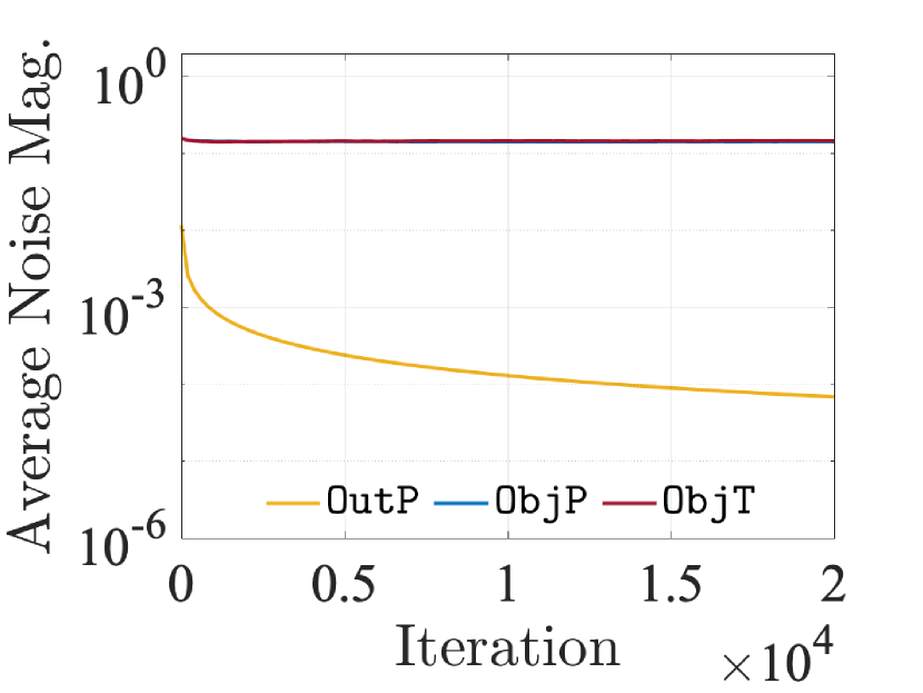
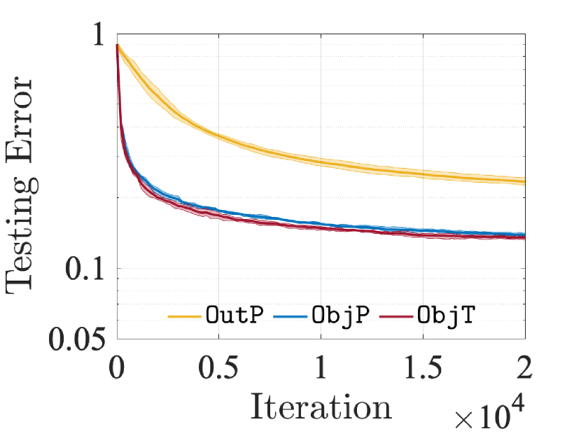
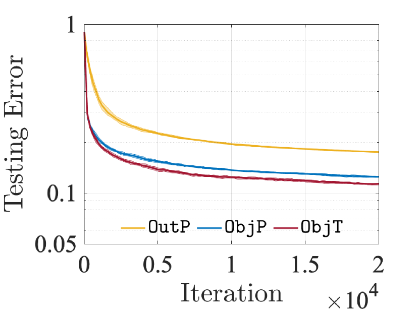
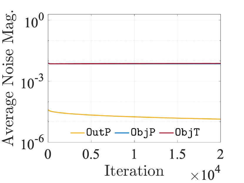
MNIST Results. Using MNIST described in Table 1, we compare the performances of ObjP, ObjT, and OutP. For each algorithm and fixed ϵ¯¯italic-ϵ\bar{\epsilon}, we generate 101010 instances, each of which has different realizations of the random noises. The random noises to OutP are generated by the Gaussian mechanism with decreasing variance as in [10], whereas the noises to our algorithms are generated by the Laplacian mechanism as in (9). To compare the two different mechanisms in terms of the magnitude of noises generated, we compute the following average noise magnitude:

1PJKp=1Pj=1Jk=1K|ξ^pjkt|,t[T],1𝑃𝐽𝐾superscriptsubscript𝑝1𝑃superscriptsubscript𝑗1𝐽superscriptsubscript𝑘1𝐾subscriptsuperscript^𝜉𝑡𝑝𝑗𝑘for-all𝑡delimited-[]𝑇\displaystyle\textstyle\frac{1}{PJK}\sum_{p=1}^{P}\sum_{j=1}^{J}\sum_{k=1}^{K}|\hat{\xi}^{t}_{pjk}|,\ \forall t\in[T],

where ξ^pjktsubscriptsuperscript^𝜉𝑡𝑝𝑗𝑘\hat{\xi}^{t}_{pjk} is a realization of random noise ξ~pjktsubscriptsuperscript~𝜉𝑡𝑝𝑗𝑘\tilde{\xi}^{t}_{pjk}.

Refer to caption
Refer to caption
(a) ϵ¯=0.05¯italic-ϵ0.05\bar{\epsilon}=0.05
Refer to caption
Refer to caption
(b) ϵ¯=0.1¯italic-ϵ0.1\bar{\epsilon}=0.1
Refer to caption
Refer to caption
(c) ϵ¯=1¯italic-ϵ1\bar{\epsilon}=1
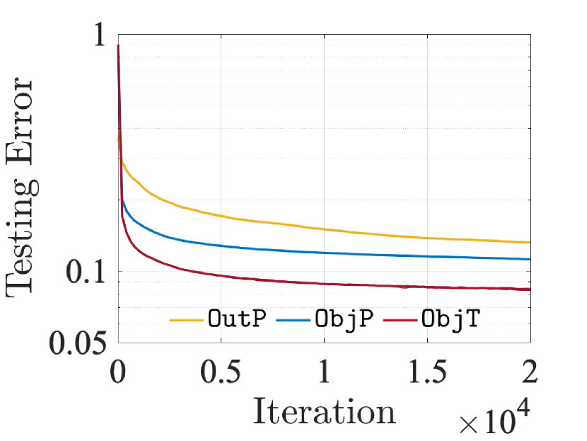
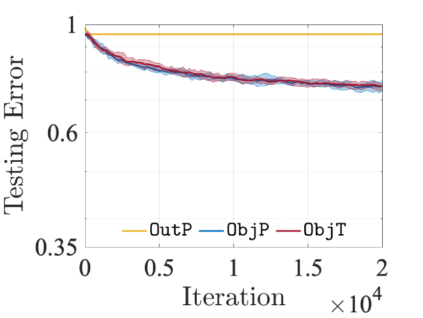
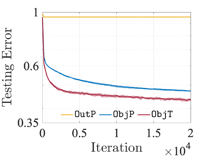
Figure 1: [MNIST] Average noise magnitudes (top) and testing errors (bottom) for every iteration.

In Figure 1, for every algorithm, ϵ¯{0.05,0.1,1}¯italic-ϵ0.050.11\bar{\epsilon}\in\{0.05,0.1,1\}, and iteration t[2e4]𝑡delimited-[]2𝑒4t\in[2e4], we report the average noise magnitudes and testing errors on average (solid line) with the 202020- and 808080-percentile confidence bounds (shaded), respectively in the top and bottom rows of the figure. We exclude the cases when ϵ¯{3,5}¯italic-ϵ35\bar{\epsilon}\in\{3,5\} in Figure 1, since ObjT provides an accurate solution even when ϵ¯=1¯italic-ϵ1\bar{\epsilon}=1. In what follows, we present some observations from the figures and their implications. The average noise magnitudes of all the algorithms increase as ϵ¯¯italic-ϵ\bar{\epsilon} decreases, achieving stronger data privacy. For fixed ϵ¯¯italic-ϵ\bar{\epsilon}, the average noise magnitudes of our algorithms ObjT and ObjP are greater than those of OutP while the testing errors of our algorithms are less than those of OutP. These results imply that the performance of our algorithms is less sensitive to the random perturbation than that of OutP, even with a larger magnitude of noises for stronger ϵ¯¯italic-ϵ\bar{\epsilon}-DP. The greater performance of our algorithms is also consistent with the findings in [5, 30] that the better performance of the objective perturbation than the output perturbation is guaranteed with higher probability. The sequence of solutions produced by our algorithms, especially ObjT, converges faster than that produced by OutP.
Refer to caption
(a) MNIST
Refer to caption
(b) FEMNIST
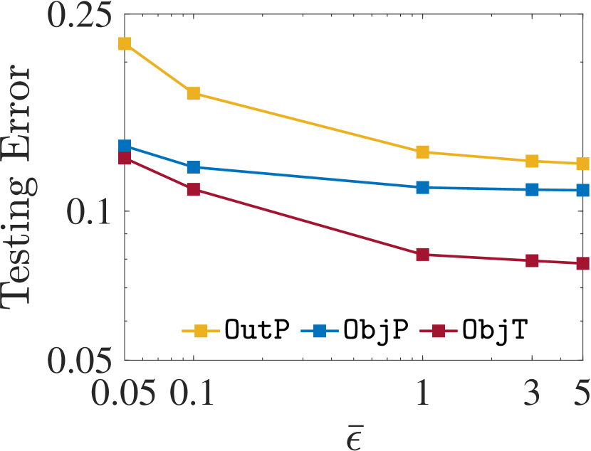
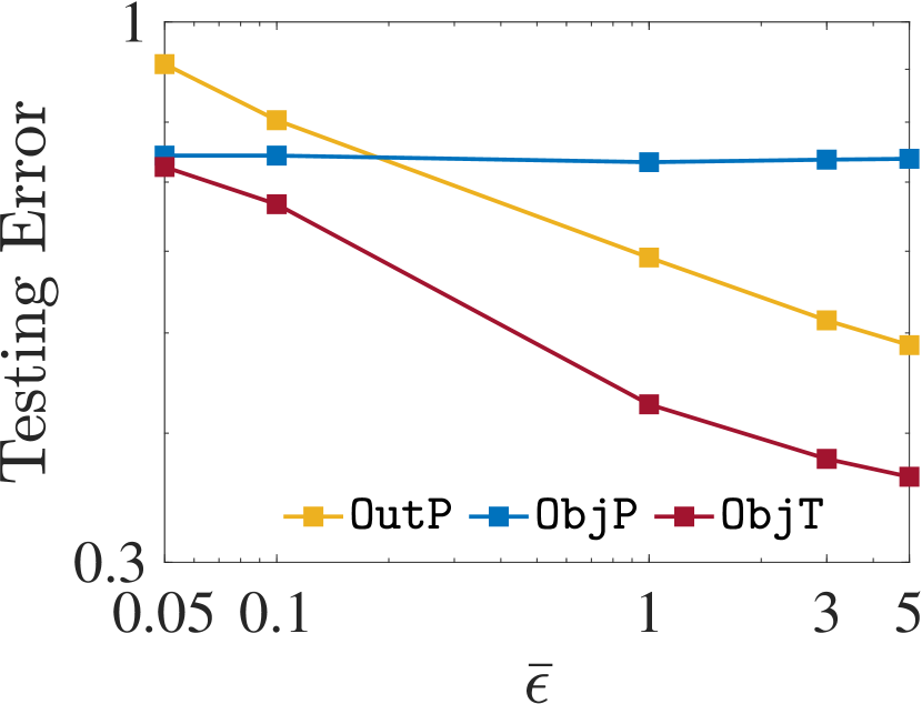
Figure 2: Testing errors of the three algorithms under various ϵ¯¯italic-ϵ\bar{\epsilon}.

In Figure 2(a) we report the testing errors of the three algorithms for every ϵ¯{0.05,0.1,1,3,5}¯italic-ϵ0.050.1135\bar{\epsilon}\in\{0.05,0.1,1,3,5\}. When ϵ¯=5¯italic-ϵ5\bar{\epsilon}=5, the testing error produced by ObjT is 7.84%percent7.847.84\%, which is close to that of a nonprivate algorithm (i.e., 7.42%percent7.427.42\%). As ϵ¯¯italic-ϵ\bar{\epsilon} decreases (i.e., stronger data privacy), the testing errors of all algorithms increase, implying a fundamental trade-off between solution accuracy and data privacy. When ϵ¯=0.05¯italic-ϵ0.05\bar{\epsilon}=0.05, the testing error of ObjT is 12.80%percent12.8012.80\% while that of OutP is 21.79%percent21.7921.79\%, an 8.99%percent8.998.99\% improvement.

Remark 3.

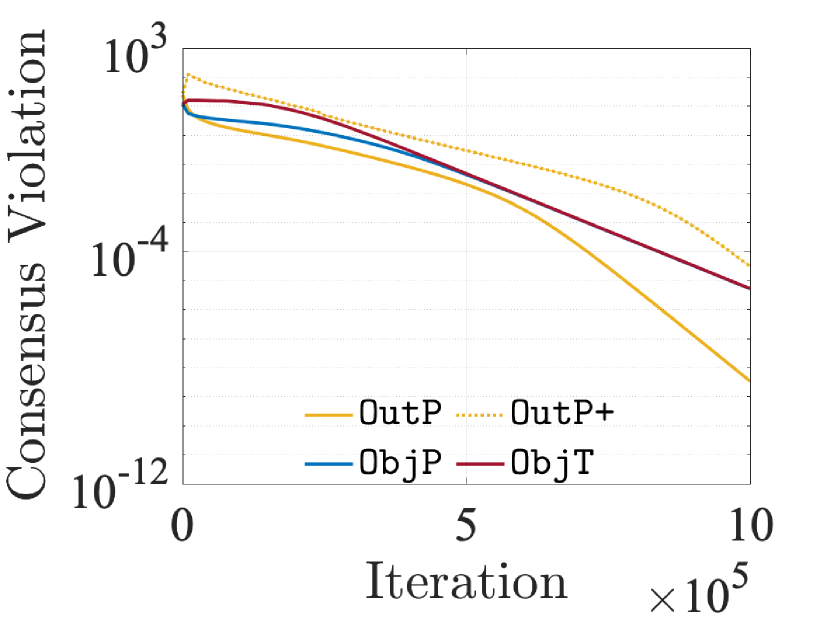
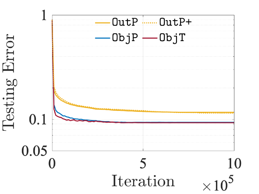
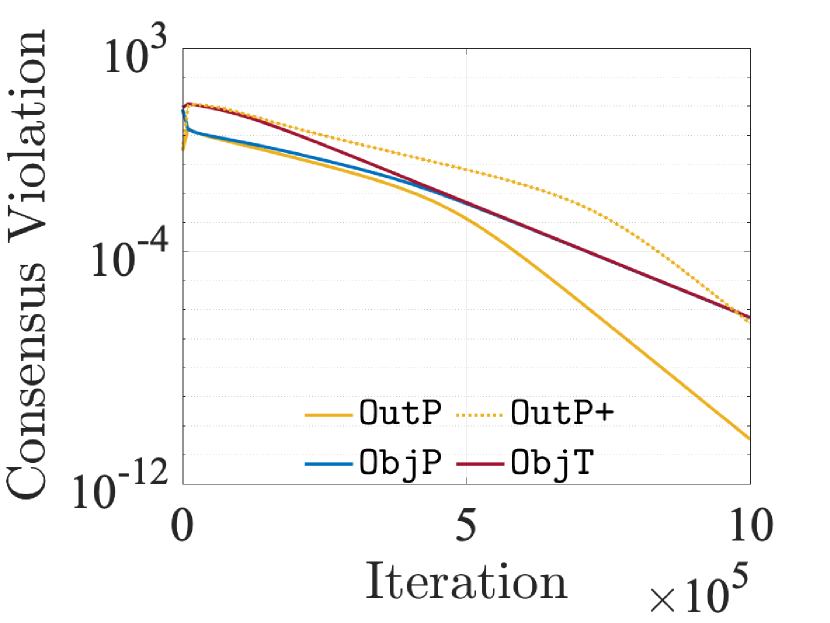
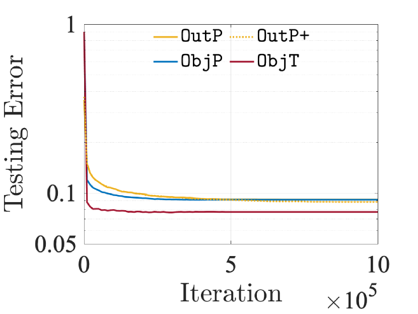
Additionally, we increase the number of iterations to T=1e6𝑇1𝑒6T=1e6 and verify that the solutions provided by the three algorithms are feasible, namely, satisfying the consensus constraints (2b) (see Appendix A.10 for more details). Under this setting, we additionally consider a case when ϵ¯=0.01¯italic-ϵ0.01\bar{\epsilon}=0.01, and we demonstrate that the testing error of OutT is 15.64%percent15.6415.64\% while that of OutP is 37.98%percent37.9837.98\%, a 22.34%percent22.3422.34\% improvement. In summary, the results demonstrate the outperformance of our algorithms.

FEMNIST Results. Using FEMNIST described in Table 1, we aim to show that our algorithms outperform OutP under the heterogeneous data setting (i.e., the number of data per agent varies).

Refer to caption
(a) ϵ¯=0.05¯italic-ϵ0.05\bar{\epsilon}=0.05
Refer to caption
(b) ϵ¯=0.1¯italic-ϵ0.1\bar{\epsilon}=0.1
Refer to caption
(c) ϵ¯=1¯italic-ϵ1\bar{\epsilon}=1
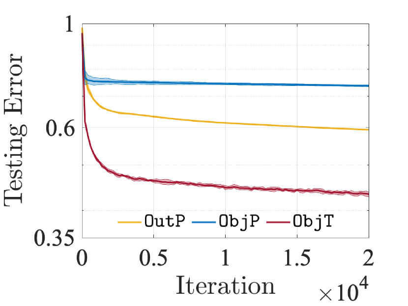
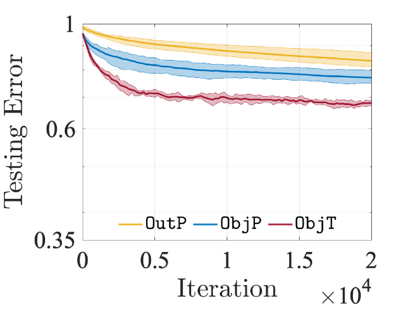
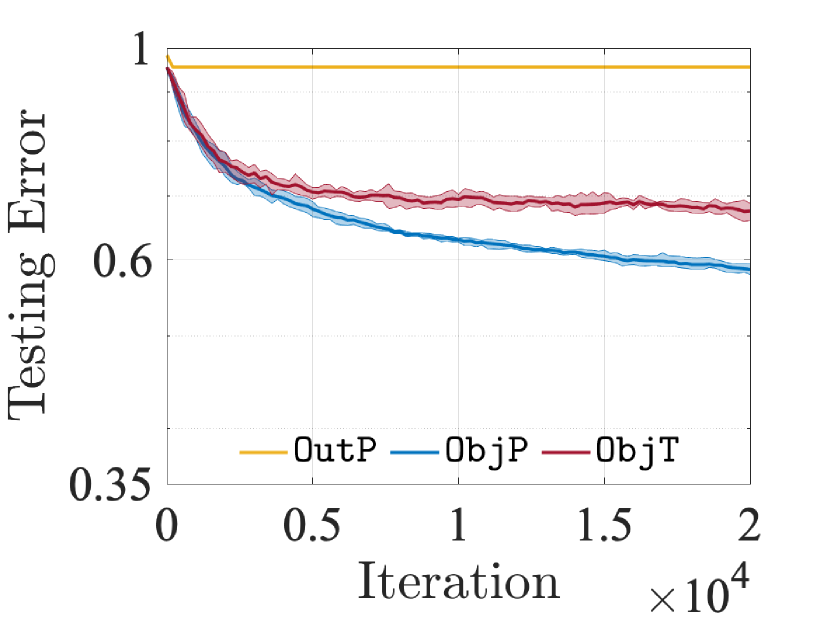
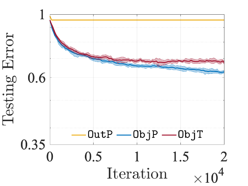
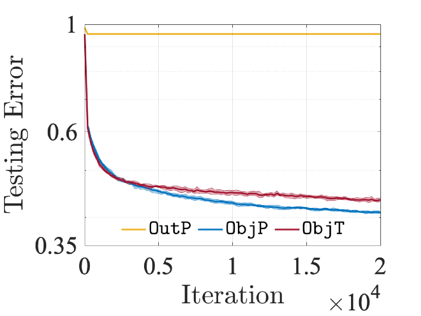
Figure 3: [FEMNIST] Testing errors for every iteration.

In Figure 3, for every algorithm, ϵ¯{0.05,0.1,1}¯italic-ϵ0.050.11\bar{\epsilon}\in\{0.05,0.1,1\}, and iteration t[2e4]𝑡delimited-[]2𝑒4t\in[2e4], we report the testing errors on average (solid line) with the 202020- and 808080-percentile confidence bounds (shaded). In what follows, we present some observations from the figures and their implications. ObjT produces the least testing error with the fastest convergence, which is similar to the result from Figure 1. When ϵ¯=1¯italic-ϵ1\bar{\epsilon}=1, the testing error of ObjP is greater than that of OutP. To see this in more detail, we also note that the effect of ϵ¯¯italic-ϵ\bar{\epsilon} on the testing error of ObjP is not significant (see also the blue line in Figure 2(b)). In Appendix A.11 we verify that ObjP requires an additional hyperparameter tuning process since the proximity is controlled in the objective function and thus affected by the other parameters, such as ρtsuperscript𝜌𝑡\rho^{t}. However, we highlight that this additional tuning process is not required for ObjT since the proximity is controlled in the constraints and thus not affected by the other parameters. Taking this viewpoint, ObjT has an additional advantage over ObjP.

In Figure 2(b) we report the testing errors of the three algorithms for every ϵ¯{0.05,0.1,1,3,5}¯italic-ϵ0.050.1135\bar{\epsilon}\in\{0.05,0.1,1,3,5\}. When ϵ¯=5¯italic-ϵ5\bar{\epsilon}=5, the testing error of ObjT is 36.29%percent36.2936.29\% which is close to that of a nonprivate algorithm (i.e., 35.25%percent35.2535.25\%). As ϵ¯¯italic-ϵ\bar{\epsilon} decreases (i.e., stronger data privacy), the testing errors of all algorithms increase, thus implying a trade-off between solution accuracy and data privacy. When ϵ¯=0.05¯italic-ϵ0.05\bar{\epsilon}=0.05, the testing error of ObjT is 72.40%percent72.4072.40\% while that of OutP is 91.05%percent91.0591.05\%, an 18.65%percent18.6518.65\% improvement.

5 Conclusion

We incorporated the objective perturbation into an IADMM algorithm for solving the FL model while ensuring data privacy during a training process. The proposed DP-IADMM algorithm iteratively solves a sequence of subproblems whose objective functions are randomly perturbed by noises sampled from a calibrated Laplace distribution to ensure ϵ¯¯italic-ϵ\bar{\epsilon}-DP. We showed that the rate of convergence in expectation for the proposed Algorithm 1 is 𝒪(1/T)𝒪1𝑇\mathcal{O}(1/\sqrt{T}) with T𝑇T being the number of iterations. In the numerical experiments, we demonstrated the outperformance of the proposed algorithm by using MNIST and FEMNIST instances.

We note that the performance of the proposed DP algorithm can be further improved by lowering the magnitude of noises required for ensuring the same level of data privacy (see Figure 1 (top) that our algorithm requires larger noises). By improving the performance further, we expect that the proposed DP algorithm can be utilized for learning from larger decentralized datasets with more features and classes.

Acknowledgments. This material was based upon work supported by the U.S. Department of Energy, Office of Science, Advanced Scientific Computing Research, under Contract DE-AC02-06CH11357. We gratefully acknowledge the computing resources provided on Swing, a high-performance computing cluster operated by the Laboratory Computing Resource Center at Argonne National Laboratory.

References

  • [1] Martin Abadi, Andy Chu, Ian Goodfellow, H Brendan McMahan, Ilya Mironov, Kunal Talwar, and Li Zhang. Deep learning with differential privacy. In Proceedings of the 2016 ACM SIGSAC conference on computer and communications security, pages 308–318, 2016.
  • [2] Naman Agarwal, Ananda Theertha Suresh, Felix Yu, Sanjiv Kumar, and H Brendan Mcmahan. cpsgd: Communication-efficient and differentially-private distributed sgd. arXiv preprint arXiv:1805.10559, 2018.
  • [3] Patrick Billingsley. Probability and measure. John Wiley & Sons, 1995.
  • [4] Sebastian Caldas, Sai Meher Karthik Duddu, Peter Wu, Tian Li, Jakub Konečnỳ, H Brendan McMahan, Virginia Smith, and Ameet Talwalkar. Leaf: A benchmark for federated settings. arXiv preprint arXiv:1812.01097, 2018.
  • [5] Kamalika Chaudhuri, Claire Monteleoni, and Anand D Sarwate. Differentially private empirical risk minimization. Journal of Machine Learning Research, 12(3), 2011.
  • [6] Cynthia Dwork, Frank McSherry, Kobbi Nissim, and Adam Smith. Calibrating noise to sensitivity in private data analysis. In Theory of cryptography conference, pages 265–284. Springer, 2006.
  • [7] Cynthia Dwork, Aaron Roth, et al. The algorithmic foundations of differential privacy. Foundations and Trends in Theoretical Computer Science, 9(3-4):211–407, 2014.
  • [8] Anis Elgabli, Jihong Park, Amrit S Bedi, Mehdi Bennis, and Vaneet Aggarwal. GADMM: Fast and communication efficient framework for distributed machine learning. Journal of Machine Learning Research, 21(76):1–39, 2020.
  • [9] Kazuto Fukuchi, Quang Khai Tran, and Jun Sakuma. Differentially private empirical risk minimization with input perturbation. In International Conference on Discovery Science, pages 82–90. Springer, 2017.
  • [10] Zonghao Huang, Rui Hu, Yuanxiong Guo, Eric Chan-Tin, and Yanmin Gong. DP-ADMM: ADMM-based distributed learning with differential privacy. IEEE Transactions on Information Forensics and Security, 15:1002–1012, 2019.
  • [11] Roger Iyengar, Joseph P Near, Dawn Song, Om Thakkar, Abhradeep Thakurta, and Lun Wang. Towards practical differentially private convex optimization. In 2019 IEEE Symposium on Security and Privacy (SP), pages 299–316. IEEE, 2019.
  • [12] Peter Kairouz, H Brendan McMahan, Brendan Avent, Aurélien Bellet, Mehdi Bennis, Arjun Nitin Bhagoji, Keith Bonawitz, Zachary Charles, Graham Cormode, Rachel Cummings, et al. Advances and open problems in federated learning. arXiv preprint arXiv:1912.04977, 2019.
  • [13] Georgios A Kaissis, Marcus R Makowski, Daniel Rückert, and Rickmer F Braren. Secure, privacy-preserving and federated machine learning in medical imaging. Nature Machine Intelligence, 2(6):305–311, 2020.
  • [14] Yilin Kang, Yong Liu, Ben Niu, Xinyi Tong, Likun Zhang, and Weiping Wang. Input perturbation: A new paradigm between central and local differential privacy. arXiv preprint arXiv:2002.08570, 2020.
  • [15] Daniel Kifer, Adam Smith, and Abhradeep Thakurta. Private convex empirical risk minimization and high-dimensional regression. In Conference on Learning Theory, pages 25–1. JMLR Workshop and Conference Proceedings, 2012.
  • [16] Jakub Konečnỳ, Brendan McMahan, and Daniel Ramage. Federated optimization: Distributed optimization beyond the datacenter. arXiv preprint arXiv:1511.03575, 2015.
  • [17] Yann LeCun. The MNIST database of handwritten digits. http://yann. lecun. com/exdb/mnist/, 1998.
  • [18] Qinbin Li, Zeyi Wen, Zhaomin Wu, Sixu Hu, Naibo Wang, Yuan Li, Xu Liu, and Bingsheng He. A survey on federated learning systems: vision, hype and reality for data privacy and protection. arXiv preprint arXiv:1907.09693, 2019.
  • [19] Qunwei Li, Bhavya Kailkhura, Ryan Goldhahn, Priyadip Ray, and Pramod K Varshney. Robust decentralized learning using ADMM with unreliable agents. arXiv preprint arXiv:1710.05241, 2017.
  • [20] Tian Li, Anit Kumar Sahu, Ameet Talwalkar, and Virginia Smith. Federated learning: Challenges, methods, and future directions. IEEE Signal Processing Magazine, 37(3):50–60, 2020.
  • [21] Tian Li, Anit Kumar Sahu, Manzil Zaheer, Maziar Sanjabi, Ameet Talwalkar, and Virginia Smith. Federated optimization in heterogeneous networks. arXiv preprint arXiv:1812.06127, 2018.
  • [22] Aleksander Madry, Aleksandar Makelov, Ludwig Schmidt, Dimitris Tsipras, and Adrian Vladu. Towards deep learning models resistant to adversarial attacks. arXiv preprint arXiv:1706.06083, 2017.
  • [23] Brendan McMahan, Eider Moore, Daniel Ramage, Seth Hampson, and Blaise Aguera y Arcas. Communication-efficient learning of deep networks from decentralized data. In Artificial Intelligence and Statistics, pages 1273–1282. PMLR, 2017.
  • [24] Mohammad Naseri, Jamie Hayes, and Emiliano De Cristofaro. Toward robustness and privacy in federated learning: Experimenting with local and central differential privacy. arXiv preprint arXiv:2009.03561, 2020.
  • [25] Anand D Sarwate and Kamalika Chaudhuri. Signal processing and machine learning with differential privacy: Algorithms and challenges for continuous data. IEEE signal processing magazine, 30(5):86–94, 2013.
  • [26] Benjamin Shickel, Patrick James Tighe, Azra Bihorac, and Parisa Rashidi. Deep EHR: a survey of recent advances in deep learning techniques for electronic health record (EHR) analysis. IEEE journal of biomedical and health informatics, 22(5):1589–1604, 2017.
  • [27] Reza Shokri, Marco Stronati, Congzheng Song, and Vitaly Shmatikov. Membership inference attacks against machine learning models. In 2017 IEEE Symposium on Security and Privacy (SP), pages 3–18. IEEE, 2017.
  • [28] Choon Hui Teo, SVN Vishwanathan, Alex Smola, and Quoc V Le. Bundle methods for regularized risk minimization. Journal of Machine Learning Research, 11(1), 2010.
  • [29] Kang Wei, Jun Li, Ming Ding, Chuan Ma, Howard H Yang, Farhad Farokhi, Shi Jin, Tony QS Quek, and H Vincent Poor. Federated learning with differential privacy: Algorithms and performance analysis. IEEE Transactions on Information Forensics and Security, 15:3454–3469, 2020.
  • [30] Tao Zhang and Quanyan Zhu. Dynamic differential privacy for ADMM-based distributed classification learning. IEEE Transactions on Information Forensics and Security, 12(1):172–187, 2016.

The submitted manuscript has been created by UChicago Argonne, LLC, Operator of Argonne National Laboratory (“Argonne”). Argonne, a U.S. Department of Energy Office of Science laboratory, is operated under Contract No. DE-AC02-06CH11357. The U.S. Government retains for itself, and others acting on its behalf, a paid-up nonexclusive, irrevocable worldwide license in said article to reproduce, prepare derivative works, distribute copies to the public, and perform publicly and display publicly, by or on behalf of the Government. The Department of Energy will provide public access to these results of federally sponsored research in accordance with the DOE Public Access Plan (http://energy.gov/downloads/doe-public-access-plan).

Appendix A Appendix

A.1 Derivation of (10)

By adding ξ~pt,zpsubscriptsuperscript~𝜉𝑡𝑝subscript𝑧𝑝\langle\tilde{\xi}^{t}_{p},z_{p}\rangle to the function (5b), we have

fp(zpt;𝒟p),zp+ρt2wt+1zp+1ρtλpt2+ξ~pt,zp.subscriptsuperscript𝑓𝑝subscriptsuperscript𝑧𝑡𝑝subscript𝒟𝑝subscript𝑧𝑝superscript𝜌𝑡2superscriptnormsuperscript𝑤𝑡1subscript𝑧𝑝1superscript𝜌𝑡subscriptsuperscript𝜆𝑡𝑝2subscriptsuperscript~𝜉𝑡𝑝subscript𝑧𝑝\displaystyle\langle f^{\prime}_{p}(z^{t}_{p};\mathcal{D}_{p}),\ z_{p}\rangle+\textstyle\frac{\rho^{t}}{2}\|w^{t+1}-z_{p}+\frac{1}{\rho^{t}}\lambda^{t}_{p}\|^{2}+\langle\tilde{\xi}^{t}_{p},z_{p}\rangle. (22)

Now we add a constant 12ρtξ~pt2wt+1+1ρtλpt,ξ~pt12superscript𝜌𝑡superscriptnormsubscriptsuperscript~𝜉𝑡𝑝2superscript𝑤𝑡11superscript𝜌𝑡subscriptsuperscript𝜆𝑡𝑝subscriptsuperscript~𝜉𝑡𝑝\frac{1}{2\rho^{t}}\|\tilde{\xi}^{t}_{p}\|^{2}-\langle w^{t+1}+\frac{1}{\rho^{t}}\lambda^{t}_{p},\tilde{\xi}^{t}_{p}\rangle to (22), yielding

fp(zpt;𝒟p),zp+ρt2wt+1zp+1ρtλpt2+12ρtξ~pt2wt+1zp+1ρtλpt,ξ~ptsubscriptsuperscript𝑓𝑝subscriptsuperscript𝑧𝑡𝑝subscript𝒟𝑝subscript𝑧𝑝superscript𝜌𝑡2superscriptnormsuperscript𝑤𝑡1subscript𝑧𝑝1superscript𝜌𝑡subscriptsuperscript𝜆𝑡𝑝212superscript𝜌𝑡superscriptnormsubscriptsuperscript~𝜉𝑡𝑝2superscript𝑤𝑡1subscript𝑧𝑝1superscript𝜌𝑡subscriptsuperscript𝜆𝑡𝑝subscriptsuperscript~𝜉𝑡𝑝\displaystyle\langle f^{\prime}_{p}(z^{t}_{p};\mathcal{D}_{p}),\ z_{p}\rangle+\textstyle\frac{\rho^{t}}{2}\|w^{t+1}-z_{p}+\frac{1}{\rho^{t}}\lambda^{t}_{p}\|^{2}+\frac{1}{2\rho^{t}}\|\tilde{\xi}^{t}_{p}\|^{2}-\langle w^{t+1}-z_{p}+\frac{1}{\rho^{t}}\lambda^{t}_{p},\tilde{\xi}^{t}_{p}\rangle
=\displaystyle= fp(zpt;𝒟p),zp+ρt2{wt+1zp+1ρtλpt2+1(ρt)2ξ~pt22ρtwt+1zp+1ρtλpt,ξ~pt}subscriptsuperscript𝑓𝑝subscriptsuperscript𝑧𝑡𝑝subscript𝒟𝑝subscript𝑧𝑝superscript𝜌𝑡2superscriptnormsuperscript𝑤𝑡1subscript𝑧𝑝1superscript𝜌𝑡subscriptsuperscript𝜆𝑡𝑝21superscriptsuperscript𝜌𝑡2superscriptnormsubscriptsuperscript~𝜉𝑡𝑝22superscript𝜌𝑡superscript𝑤𝑡1subscript𝑧𝑝1superscript𝜌𝑡subscriptsuperscript𝜆𝑡𝑝subscriptsuperscript~𝜉𝑡𝑝\displaystyle\langle f^{\prime}_{p}(z^{t}_{p};\mathcal{D}_{p}),\ z_{p}\rangle+\textstyle\frac{\rho^{t}}{2}\Big{\{}\|w^{t+1}-z_{p}+\frac{1}{\rho^{t}}\lambda^{t}_{p}\|^{2}+\frac{1}{(\rho^{t})^{2}}\|\tilde{\xi}^{t}_{p}\|^{2}-\frac{2}{\rho^{t}}\langle w^{t+1}-z_{p}+\frac{1}{\rho^{t}}\lambda^{t}_{p},\tilde{\xi}^{t}_{p}\rangle\Big{\}}
=\displaystyle= fp(zpt;𝒟p),zp+ρt2wt+1zp+1ρtλpt1ρtξ~pt2,subscriptsuperscript𝑓𝑝subscriptsuperscript𝑧𝑡𝑝subscript𝒟𝑝subscript𝑧𝑝superscript𝜌𝑡2superscriptnormsuperscript𝑤𝑡1subscript𝑧𝑝1superscript𝜌𝑡subscriptsuperscript𝜆𝑡𝑝1superscript𝜌𝑡subscriptsuperscript~𝜉𝑡𝑝2\displaystyle\langle f^{\prime}_{p}(z^{t}_{p};\mathcal{D}_{p}),\ z_{p}\rangle+\textstyle\frac{\rho^{t}}{2}\|w^{t+1}-z_{p}+\frac{1}{\rho^{t}}\lambda^{t}_{p}-\frac{1}{\rho^{t}}\tilde{\xi}^{t}_{p}\|^{2},

which is equivalent to (10).

A.2 Proof of Proposition 1

Fix t𝑡t and p𝑝p. We denote by z^pt+1subscriptsuperscript^𝑧𝑡1𝑝\hat{z}^{t+1}_{p} (resp., z^pt+1subscriptsuperscript^𝑧𝑡1𝑝\hat{z}^{t+1}_{p\ell}) the unique optimal solution of an optimization problem in (8) (resp., (14)), where the uniqueness is due to the strong convexity of the objective functions. For ease of exposition, we define Gpt(zp):=Gt(zp;𝒟p,ξ~pt)+(1/2ηt)zpzpt2assignsubscriptsuperscript𝐺𝑡𝑝subscript𝑧𝑝superscript𝐺𝑡subscript𝑧𝑝subscript𝒟𝑝subscriptsuperscript~𝜉𝑡𝑝12superscript𝜂𝑡superscriptnormsubscript𝑧𝑝superscriptsubscript𝑧𝑝𝑡2G^{t}_{p}(z_{p}):=G^{t}(z_{p};\mathcal{D}_{p},\tilde{\xi}^{t}_{p})+(1/2\eta^{t})\|z_{p}-z_{p}^{t}\|^{2} and gp(zp):=g(zp;)assignsubscript𝑔𝑝subscript𝑧𝑝𝑔subscript𝑧𝑝g_{p\ell}(z_{p}):=g(z_{p};\ell).

In (8), the continuity of Gpt:𝒲:subscriptsuperscript𝐺𝑡𝑝maps-to𝒲G^{t}_{p}:\mathcal{W}\mapsto\mathbb{R} at z^pt+1subscriptsuperscript^𝑧𝑡1𝑝\hat{z}^{t+1}_{p} implies that, for every ϵ>0italic-ϵ0\epsilon>0, there exists a δ>0𝛿0\delta>0 such that for all z𝒲𝑧𝒲z\in\mathcal{W}:

zδ(z^pt+1):={zJ×K:zz^pt+1<δ}Gpt(z)Gpt(z^pt+1)<ϵ.𝑧subscript𝛿subscriptsuperscript^𝑧𝑡1𝑝assignconditional-set𝑧superscript𝐽𝐾norm𝑧subscriptsuperscript^𝑧𝑡1𝑝𝛿subscriptsuperscript𝐺𝑡𝑝𝑧subscriptsuperscript𝐺𝑡𝑝subscriptsuperscript^𝑧𝑡1𝑝italic-ϵ\displaystyle z\in\mathcal{B}_{\delta}(\hat{z}^{t+1}_{p}):=\{z\in\mathbb{R}^{J\times K}:\|z-\hat{z}^{t+1}_{p}\|<\delta\}\ \Rightarrow\ G^{t}_{p}(z)-G^{t}_{p}(\hat{z}^{t+1}_{p})<\epsilon. (23a)
Consider z~δ(z^pt+1)relint(𝒲)~𝑧subscript𝛿subscriptsuperscript^𝑧𝑡1𝑝relint𝒲\tilde{z}\in\mathcal{B}_{\delta}(\hat{z}^{t+1}_{p})\cap\textbf{relint}(\mathcal{W}), where relint indicates the relative interior. As hm(z~)<0subscript𝑚~𝑧0h_{m}(\tilde{z})<0 for all m[M]𝑚delimited-[]𝑀m\in[M], gp(z~)subscript𝑔𝑝~𝑧g_{p\ell}(\tilde{z}) goes to zero as \ell increases. Hence, there exists >0superscript0\ell^{\prime}>0 such that
gp(z~)=m=1Mln(1+ehm(z~))<ϵ,.formulae-sequencesubscript𝑔𝑝~𝑧superscriptsubscript𝑚1𝑀1superscript𝑒subscript𝑚~𝑧italic-ϵfor-allsuperscript\displaystyle g_{p\ell}(\tilde{z})=\textstyle\sum_{m=1}^{M}\ln(1+e^{\ell h_{m}(\tilde{z})})<\epsilon,\ \forall\ell\geq\ell^{\prime}. (23b)
For all superscript\ell\geq\ell^{\prime}, we derive the following inequalities:
Gpt(z^pt+1)+gp(z^pt+1)Gpt(z~)+gp(z~)<Gpt(z~)+ϵ<Gpt(z^pt+1)+2ϵsubscriptsuperscript𝐺𝑡𝑝subscriptsuperscript^𝑧𝑡1𝑝subscript𝑔𝑝subscriptsuperscript^𝑧𝑡1𝑝subscriptsuperscript𝐺𝑡𝑝~𝑧subscript𝑔𝑝~𝑧subscriptsuperscript𝐺𝑡𝑝~𝑧italic-ϵsubscriptsuperscript𝐺𝑡𝑝subscriptsuperscript^𝑧𝑡1𝑝2italic-ϵ\displaystyle G^{t}_{p}(\hat{z}^{t+1}_{p\ell})+g_{p\ell}(\hat{z}^{t+1}_{p\ell})\leq G^{t}_{p}(\tilde{z})+g_{p\ell}(\tilde{z})<G^{t}_{p}(\tilde{z})+\epsilon<G^{t}_{p}(\hat{z}^{t+1}_{p})+2\epsilon (23c)

where the first inequality holds because z^pt+1subscriptsuperscript^𝑧𝑡1𝑝\hat{z}^{t+1}_{p\ell} is the optimal solution of (14), the second inequality holds by (23b), and the last inequality holds by (23a). The inequalities (23c) imply that, for very small ϵ0italic-ϵ0\epsilon\approx 0, the optimal value Gpt(z^pt+1)+gp(z^pt+1)subscriptsuperscript𝐺𝑡𝑝subscriptsuperscript^𝑧𝑡1𝑝subscript𝑔𝑝subscriptsuperscript^𝑧𝑡1𝑝G^{t}_{p}(\hat{z}^{t+1}_{p\ell})+g_{p\ell}(\hat{z}^{t+1}_{p\ell}) of (14) converges to the optimal value Gpt(z^pt+1)subscriptsuperscript𝐺𝑡𝑝subscriptsuperscript^𝑧𝑡1𝑝G^{t}_{p}(\hat{z}^{t+1}_{p}) of (8) as \ell increases.

It remains to show that z^pt+1subscriptsuperscript^𝑧𝑡1𝑝\hat{z}^{t+1}_{p\ell} converges to z^pt+1subscriptsuperscript^𝑧𝑡1𝑝\hat{z}^{t+1}_{p} as \ell increases. Suppose that z^pt+1subscriptsuperscript^𝑧𝑡1𝑝\hat{z}^{t+1}_{p\ell} converges to z^z^pt+1^𝑧subscriptsuperscript^𝑧𝑡1𝑝\widehat{z}\neq\hat{z}^{t+1}_{p} as \ell increases. Consider ζ:=z^z^pt+1/2assign𝜁norm^𝑧subscriptsuperscript^𝑧𝑡1𝑝2\zeta:=\|\widehat{z}-\hat{z}^{t+1}_{p}\|/2. Since z^pt+1subscriptsuperscript^𝑧𝑡1𝑝\hat{z}^{t+1}_{p\ell} converges to z^^𝑧\widehat{z}, there exists ′′>0superscript′′0\ell^{\prime\prime}>0 such that z^z^pt+1<ζnorm^𝑧subscriptsuperscript^𝑧𝑡1𝑝𝜁\|\widehat{z}-\hat{z}^{t+1}_{p\ell}\|<\zeta for all ′′superscript′′\ell\geq\ell^{\prime\prime}. By the triangle inequality, we have

z^pt+1z^pt+1z^z^pt+1z^z^pt+1>2ζζ=ζ,′′.formulae-sequencenormsubscriptsuperscript^𝑧𝑡1𝑝subscriptsuperscript^𝑧𝑡1𝑝norm^𝑧subscriptsuperscript^𝑧𝑡1𝑝norm^𝑧subscriptsuperscript^𝑧𝑡1𝑝2𝜁𝜁𝜁for-allsuperscript′′\displaystyle\|\hat{z}^{t+1}_{p\ell}-\hat{z}^{t+1}_{p}\|\geq\|\widehat{z}-\hat{z}^{t+1}_{p}\|-\|\widehat{z}-\hat{z}^{t+1}_{p\ell}\|>2\zeta-\zeta=\zeta,\ \forall\ell\geq\ell^{\prime\prime}. (24a)
As Gptsubscriptsuperscript𝐺𝑡𝑝G^{t}_{p} is strongly convex with a constant ρmin>0superscript𝜌min0\rho^{\text{\tiny min}}>0, we have
Gpt(z^pt+1)Gpt(z^pt+1)ρmin2z^pt+1z^pt+12>ρminζ22,′′,formulae-sequencesubscriptsuperscript𝐺𝑡𝑝subscriptsuperscript^𝑧𝑡1𝑝subscriptsuperscript𝐺𝑡𝑝subscriptsuperscript^𝑧𝑡1𝑝superscript𝜌min2superscriptnormsubscriptsuperscript^𝑧𝑡1𝑝subscriptsuperscript^𝑧𝑡1𝑝2superscript𝜌minsuperscript𝜁22for-allsuperscript′′\displaystyle G^{t}_{p}(\hat{z}^{t+1}_{p\ell})-G^{t}_{p}(\hat{z}^{t+1}_{p})\geq\textstyle\frac{\rho^{\text{\tiny min}}}{2}\|\hat{z}^{t+1}_{p\ell}-\hat{z}^{t+1}_{p}\|^{2}>\frac{\rho^{\text{\tiny min}}\zeta^{2}}{2},\ \forall\ell\geq\ell^{\prime\prime}, (24b)
where the last inequality holds by (24a). By adding gp(z^pt+1)0subscript𝑔𝑝subscriptsuperscript^𝑧𝑡1𝑝0g_{p\ell}(\hat{z}^{t+1}_{p\ell})\geq 0 to both sides of (24b), we derive the following inequality:
{Gpt(z^pt+1)+gp(z^pt+1)}Gpt(z^pt+1)>ρminζ22+gp(z^pt+1),′′,formulae-sequencesubscriptsuperscript𝐺𝑡𝑝subscriptsuperscript^𝑧𝑡1𝑝subscript𝑔𝑝subscriptsuperscript^𝑧𝑡1𝑝subscriptsuperscript𝐺𝑡𝑝subscriptsuperscript^𝑧𝑡1𝑝superscript𝜌minsuperscript𝜁22subscript𝑔𝑝subscriptsuperscript^𝑧𝑡1𝑝for-allsuperscript′′\displaystyle\big{\{}G^{t}_{p}(\hat{z}^{t+1}_{p\ell})+g_{p\ell}(\hat{z}^{t+1}_{p\ell})\big{\}}-G^{t}_{p}(\hat{z}^{t+1}_{p})>\textstyle\frac{\rho^{\text{\tiny min}}\zeta^{2}}{2}+g_{p\ell}(\hat{z}^{t+1}_{p\ell}),\ \forall\ell\geq\ell^{\prime\prime}, (24c)
which contradicts that the optimal value Gpt(z^pt+1)+gp(z^pt+1)subscriptsuperscript𝐺𝑡𝑝subscriptsuperscript^𝑧𝑡1𝑝subscript𝑔𝑝subscriptsuperscript^𝑧𝑡1𝑝G^{t}_{p}(\hat{z}^{t+1}_{p\ell})+g_{p\ell}(\hat{z}^{t+1}_{p\ell}) of (14) converges to the optimal value Gpt(z^pt+1)subscriptsuperscript𝐺𝑡𝑝subscriptsuperscript^𝑧𝑡1𝑝G^{t}_{p}(\hat{z}^{t+1}_{p}) of (8) as \ell increases. This completes the proof.

A.3 Proof of Proposition 2

Fix t𝑡t, p𝑝p, and \ell. It suffices to show that the following is true:

eϵ¯pdf(zpt+1(;𝒟p)=α)pdf(zpt+1(;𝒟p)=α)eϵ¯pdf(zpt+1(;𝒟p)=α),αJ×K,formulae-sequencesuperscript𝑒¯italic-ϵpdfsubscriptsuperscript𝑧𝑡1𝑝subscriptsuperscript𝒟𝑝𝛼pdfsubscriptsuperscript𝑧𝑡1𝑝subscript𝒟𝑝𝛼superscript𝑒¯italic-ϵpdfsubscriptsuperscript𝑧𝑡1𝑝subscriptsuperscript𝒟𝑝𝛼for-all𝛼superscript𝐽𝐾\displaystyle e^{-\bar{\epsilon}}\ \textbf{pdf}\big{(}z^{t+1}_{p}(\ell;\mathcal{D}^{\prime}_{p})=\alpha\big{)}\leq\textbf{pdf}\big{(}z^{t+1}_{p}(\ell;\mathcal{D}_{p})=\alpha\big{)}\leq e^{\bar{\epsilon}}\ \textbf{pdf}\big{(}z^{t+1}_{p}(\ell;\mathcal{D}^{\prime}_{p})=\alpha\big{)},\ \forall\alpha\in\mathbb{R}^{J\times K}, (25a)
where pdf represents a probability density function.

Consider an αJ×K𝛼superscript𝐽𝐾\alpha\in\mathbb{R}^{J\times K}. If we have zpt+1(;𝒟p)=αsubscriptsuperscript𝑧𝑡1𝑝subscript𝒟𝑝𝛼z^{t+1}_{p}(\ell;\mathcal{D}_{p})=\alpha, then α𝛼\alpha is the unique minimizer of (14) because the objective function in (14) is strongly convex. Setting the gradient of the objective function in (14) to zero yields

ξ~pt(α;𝒟p)=subscriptsuperscript~𝜉𝑡𝑝𝛼subscript𝒟𝑝absent\displaystyle\tilde{\xi}^{t}_{p}(\alpha;\mathcal{D}_{p})= fp(zpt;𝒟p)+ρt(wt+1α)+λptg(α;)1ηt(αzpt),subscriptsuperscript𝑓𝑝subscriptsuperscript𝑧𝑡𝑝subscript𝒟𝑝superscript𝜌𝑡superscript𝑤𝑡1𝛼subscriptsuperscript𝜆𝑡𝑝𝑔𝛼1superscript𝜂𝑡𝛼superscriptsubscript𝑧𝑝𝑡\displaystyle-f^{\prime}_{p}(z^{t}_{p};\mathcal{D}_{p})+\rho^{t}(w^{t+1}-\alpha)+\lambda^{t}_{p}-\nabla g(\alpha;\ell)-\textstyle\frac{1}{\eta^{t}}\big{(}\alpha-z_{p}^{t}\big{)}, (25b)

where g(α;)=m=1Mehm(α)1+ehm(α)hm(α)𝑔𝛼superscriptsubscript𝑚1𝑀superscript𝑒subscript𝑚𝛼1superscript𝑒subscript𝑚𝛼subscript𝑚𝛼\nabla g(\alpha;\ell)=\sum_{m=1}^{M}\frac{\ell e^{\ell h_{m}(\alpha)}}{1+e^{\ell h_{m}(\alpha)}}\nabla h_{m}(\alpha). Therefore, the relation between α𝛼\alpha and ξ~ptsubscriptsuperscript~𝜉𝑡𝑝\tilde{\xi}^{t}_{p} is bijective, which enables us to utilize the inverse function theorem (Theorem 17.2 in [3]), namely

pdf(zpt+1(;𝒟p)=α)|det[ξ~pt(α;𝒟p)]|=L(ξ~pt(α;𝒟p);ϵ¯,Δ¯pt),pdfsubscriptsuperscript𝑧𝑡1𝑝subscript𝒟𝑝𝛼detdelimited-[]subscriptsuperscript~𝜉𝑡𝑝𝛼subscript𝒟𝑝𝐿subscriptsuperscript~𝜉𝑡𝑝𝛼subscript𝒟𝑝¯italic-ϵsuperscriptsubscript¯Δ𝑝𝑡\displaystyle\textbf{pdf}\big{(}z^{t+1}_{p}(\ell;\mathcal{D}_{p})=\alpha\big{)}\cdot\big{|}\textbf{det}[\nabla\tilde{\xi}^{t}_{p}(\alpha;\mathcal{D}_{p})]\big{|}=L\big{(}\tilde{\xi}^{t}_{p}(\alpha;\mathcal{D}_{p});\bar{\epsilon},\bar{\Delta}_{p}^{t}\big{)}, (25c)

where det represents a determinant of a matrix, L𝐿L is from (11a), and ξ~pt(α;𝒟p)subscriptsuperscript~𝜉𝑡𝑝𝛼subscript𝒟𝑝\nabla\tilde{\xi}^{t}_{p}(\alpha;\mathcal{D}_{p}) represents a Jacobian matrix of the mapping from α𝛼\alpha to ξ~ptsubscriptsuperscript~𝜉𝑡𝑝\tilde{\xi}^{t}_{p}, namely

ξ~pt(α;𝒟p)=(ρt1/ηt)𝕀JK(m=1Mehm(α)1+ehm(α)hm(α)),subscriptsuperscript~𝜉𝑡𝑝𝛼subscript𝒟𝑝superscript𝜌𝑡1superscript𝜂𝑡subscript𝕀𝐽𝐾superscriptsubscript𝑚1𝑀superscript𝑒subscript𝑚𝛼1superscript𝑒subscript𝑚𝛼subscript𝑚𝛼\displaystyle\nabla\tilde{\xi}^{t}_{p}(\alpha;\mathcal{D}_{p})=(-\rho^{t}-1/\eta^{t})\mathbb{I}_{JK}-\nabla\Big{(}\sum_{m=1}^{M}\frac{\ell e^{\ell h_{m}(\alpha)}}{1+e^{\ell h_{m}(\alpha)}}\nabla h_{m}(\alpha)\Big{)}, (25d)

where 𝕀JKsubscript𝕀𝐽𝐾\mathbb{I}_{JK} is an identity matrix of JK×JK𝐽𝐾𝐽𝐾JK\times JK dimensions. As the Jacobian matrix is not affected by the dataset, we have

ξ~pt(α;𝒟p)=ξ~pt(α;𝒟p).subscriptsuperscript~𝜉𝑡𝑝𝛼subscript𝒟𝑝subscriptsuperscript~𝜉𝑡𝑝𝛼subscriptsuperscript𝒟𝑝\displaystyle\nabla\tilde{\xi}^{t}_{p}(\alpha;\mathcal{D}_{p})=\nabla\tilde{\xi}^{t}_{p}(\alpha;\mathcal{D}^{\prime}_{p}). (25e)

Based on (25c) and (25e), we derive the following inequalities:

pdf(zpt+1(;𝒟p)=α)pdf(zpt+1(;𝒟p)=α)=L(ξ~pt(α;𝒟p);ϵ¯,Δ¯pt)L(ξ~pt(α;𝒟p);ϵ¯,Δ¯pt)|det[ξ~pt(α;𝒟p)]||det[ξ~pt(α;𝒟p)]|=L(ξ~pt(α;𝒟p);ϵ¯,Δ¯pt)L(ξ~pt(α;𝒟p);ϵ¯,Δ¯pt)pdfsubscriptsuperscript𝑧𝑡1𝑝subscript𝒟𝑝𝛼pdfsubscriptsuperscript𝑧𝑡1𝑝subscriptsuperscript𝒟𝑝𝛼𝐿subscriptsuperscript~𝜉𝑡𝑝𝛼subscript𝒟𝑝¯italic-ϵsuperscriptsubscript¯Δ𝑝𝑡𝐿subscriptsuperscript~𝜉𝑡𝑝𝛼subscriptsuperscript𝒟𝑝¯italic-ϵsuperscriptsubscript¯Δ𝑝𝑡detdelimited-[]subscriptsuperscript~𝜉𝑡𝑝𝛼subscriptsuperscript𝒟𝑝detdelimited-[]subscriptsuperscript~𝜉𝑡𝑝𝛼subscript𝒟𝑝𝐿subscriptsuperscript~𝜉𝑡𝑝𝛼subscript𝒟𝑝¯italic-ϵsuperscriptsubscript¯Δ𝑝𝑡𝐿subscriptsuperscript~𝜉𝑡𝑝𝛼subscriptsuperscript𝒟𝑝¯italic-ϵsuperscriptsubscript¯Δ𝑝𝑡\displaystyle\frac{\textbf{pdf}\big{(}z^{t+1}_{p}(\ell;\mathcal{D}_{p})=\alpha\big{)}}{\textbf{pdf}\big{(}z^{t+1}_{p}(\ell;\mathcal{D}^{\prime}_{p})=\alpha\big{)}}=\frac{L\big{(}\tilde{\xi}^{t}_{p}(\alpha;\mathcal{D}_{p});\bar{\epsilon},\bar{\Delta}_{p}^{t}\big{)}}{L\big{(}\tilde{\xi}^{t}_{p}(\alpha;\mathcal{D}^{\prime}_{p});\bar{\epsilon},\bar{\Delta}_{p}^{t}\big{)}}\cdot\frac{\big{|}\textbf{det}[\nabla\tilde{\xi}^{t}_{p}(\alpha;\mathcal{D}^{\prime}_{p})]\big{|}}{\big{|}\textbf{det}[\nabla\tilde{\xi}^{t}_{p}(\alpha;\mathcal{D}_{p})]\big{|}}=\frac{L\big{(}\tilde{\xi}^{t}_{p}(\alpha;\mathcal{D}_{p});\bar{\epsilon},\bar{\Delta}_{p}^{t}\big{)}}{L\big{(}\tilde{\xi}^{t}_{p}(\alpha;\mathcal{D}^{\prime}_{p});\bar{\epsilon},\bar{\Delta}_{p}^{t}\big{)}}
=exp((ϵ¯/Δ¯pt)(ξ~pt(α;𝒟p)1ξ~pt(α;𝒟p)1))exp((ϵ¯/Δ¯pt)(ξ~pt(α;𝒟p)ξ~pt(α;𝒟p)1))absentexp¯italic-ϵsuperscriptsubscript¯Δ𝑝𝑡subscriptnormsubscriptsuperscript~𝜉𝑡𝑝𝛼subscriptsuperscript𝒟𝑝1subscriptnormsubscriptsuperscript~𝜉𝑡𝑝𝛼subscript𝒟𝑝1exp¯italic-ϵsuperscriptsubscript¯Δ𝑝𝑡subscriptnormsubscriptsuperscript~𝜉𝑡𝑝𝛼subscriptsuperscript𝒟𝑝subscriptsuperscript~𝜉𝑡𝑝𝛼subscript𝒟𝑝1\displaystyle=\textbf{exp}\Big{(}(\bar{\epsilon}/\bar{\Delta}_{p}^{t})(\|\tilde{\xi}^{t}_{p}(\alpha;\mathcal{D}^{\prime}_{p})\|_{1}-\|\tilde{\xi}^{t}_{p}(\alpha;\mathcal{D}_{p})\|_{1})\Big{)}\leq\textbf{exp}\Big{(}(\bar{\epsilon}/\bar{\Delta}_{p}^{t})(\|\tilde{\xi}^{t}_{p}(\alpha;\mathcal{D}^{\prime}_{p})-\tilde{\xi}^{t}_{p}(\alpha;\mathcal{D}_{p})\|_{1})\Big{)}
=exp((ϵ¯/Δ¯pt)(fp(zpt;𝒟p)fp(zpt;𝒟p)1))exp(ϵ¯),absentexp¯italic-ϵsuperscriptsubscript¯Δ𝑝𝑡subscriptnormsubscriptsuperscript𝑓𝑝subscriptsuperscript𝑧𝑡𝑝subscript𝒟𝑝subscriptsuperscript𝑓𝑝subscriptsuperscript𝑧𝑡𝑝subscriptsuperscript𝒟𝑝1exp¯italic-ϵ\displaystyle=\textbf{exp}\Big{(}(\bar{\epsilon}/\bar{\Delta}_{p}^{t})(\|f^{\prime}_{p}(z^{t}_{p};\mathcal{D}_{p})-f^{\prime}_{p}(z^{t}_{p};\mathcal{D}^{\prime}_{p})\|_{1})\Big{)}\leq\textbf{exp}(\bar{\epsilon}),

where exp represents the exponential function, the first equality is from (25c), the second equality holds because of (25e), the first inequality holds because of the reverse triangle inequality, the last equality holds because of (25b), and the last inequality holds because of (11b). Similarly, one can derive a lower bound in (25a). Integrating α𝛼\alpha in (25a) over 𝒮𝒮\mathcal{S} yields (15). This completes the proof.

A.4 Privacy Analsis for Algorithm 2

Using Lemma 1, we will show that the constrained problem (9) provides ϵ¯¯italic-ϵ\bar{\epsilon}-DP. For the rest of this section, we fix t𝑡t\in\mathbb{N} and p[P]𝑝delimited-[]𝑃p\in[P]. For ease of exposition, we express the feasible region of (9) using M𝑀M inequalities, namely,

{𝒲𝒲^pt}{zpJ×K:hmt(zp)0,m[M]},𝒲subscriptsuperscript^𝒲𝑡𝑝conditional-setsubscript𝑧𝑝superscript𝐽𝐾formulae-sequencesuperscriptsubscript𝑚𝑡subscript𝑧𝑝0for-all𝑚delimited-[]𝑀\displaystyle\{\mathcal{W}\cap\widehat{\mathcal{W}}^{t}_{p}\}\Leftrightarrow\{z_{p}\in\mathbb{R}^{J\times K}:h_{m}^{t}(z_{p})\leq 0,\ \forall m\in[M]\},

where hmtsuperscriptsubscript𝑚𝑡h_{m}^{t} is convex and twice continuously differentiable.

Similar to the unconstrained problem (14), we construct the following unconstrained problem:

zpt+1(,𝒟p)=argminzpJ×KGt(zp;𝒟p,ξ~pt)+gt(zp;),subscriptsuperscript𝑧𝑡1𝑝subscript𝒟𝑝subscriptargminsubscript𝑧𝑝superscript𝐽𝐾superscript𝐺𝑡subscript𝑧𝑝subscript𝒟𝑝subscriptsuperscript~𝜉𝑡𝑝superscript𝑔𝑡subscript𝑧𝑝\displaystyle z^{t+1}_{p}(\ell,\mathcal{D}_{p})=\textstyle\operatorname*{arg\,min}_{z_{p}\in\mathbb{R}^{J\times K}}\ G^{t}(z_{p};\mathcal{D}_{p},\tilde{\xi}^{t}_{p})+g^{t}(z_{p};\ell), (26a)
gt(zp;):=m=1Mln(1+ehmt(zp)),assignsuperscript𝑔𝑡subscript𝑧𝑝superscriptsubscript𝑚1𝑀1superscript𝑒superscriptsubscript𝑚𝑡subscript𝑧𝑝\displaystyle g^{t}(z_{p};\ell):=\textstyle\sum_{m=1}^{M}\ln(1+e^{\ell h_{m}^{t}(z_{p})}), (26b)

where >00\ell>0.

We will show that (26) satisfies the pointwise convergence condition and provides ϵ¯¯italic-ϵ\bar{\epsilon}-DP as in Propositions 4 and 5, respectively.

Proposition 4.

For fixed t𝑡t and p𝑝p, we have limzpt+1(,𝒟p)=zpt+1(𝒟p)subscriptsuperscriptsubscript𝑧𝑝𝑡1subscript𝒟𝑝superscriptsubscript𝑧𝑝𝑡1subscript𝒟𝑝\lim_{\ell\rightarrow\infty}z_{p}^{t+1}(\ell,\mathcal{D}_{p})=z_{p}^{t+1}(\mathcal{D}_{p}), where zpt+1(𝒟p)superscriptsubscript𝑧𝑝𝑡1subscript𝒟𝑝z_{p}^{t+1}(\mathcal{D}_{p}) and zpt+1(,𝒟p)superscriptsubscript𝑧𝑝𝑡1subscript𝒟𝑝z_{p}^{t+1}(\ell,\mathcal{D}_{p}) are from (9) and (26), respectively.

Proof.

Fix t𝑡t and p𝑝p. Suppose that z^pt+1subscriptsuperscript^𝑧𝑡1𝑝\hat{z}^{t+1}_{p} (resp., z^pt+1subscriptsuperscript^𝑧𝑡1𝑝\hat{z}^{t+1}_{p\ell}) is the unique optimal solution of an optimization problem in (9) (resp., (26)). One can follow the proof in Appendix A.2 by setting Gpt(zp):=Gt(zp;𝒟p,ξ~pt)assignsubscriptsuperscript𝐺𝑡𝑝subscript𝑧𝑝superscript𝐺𝑡subscript𝑧𝑝subscript𝒟𝑝subscriptsuperscript~𝜉𝑡𝑝G^{t}_{p}(z_{p}):=G^{t}(z_{p};\mathcal{D}_{p},\tilde{\xi}^{t}_{p}) and gp(zp):=gt(zp;)assignsubscript𝑔𝑝subscript𝑧𝑝superscript𝑔𝑡subscript𝑧𝑝g_{p\ell}(z_{p}):=g^{t}(z_{p};\ell). ∎

Proposition 5.

For fixed t𝑡t, p𝑝p, and \ell, (26) provides ϵ¯¯italic-ϵ\bar{\epsilon}-DP, namely, satisfying

eϵ¯(zpt+1(;𝒟p)𝒮)(zpt+1(;𝒟p)𝒮)eϵ¯(zpt+1(;𝒟p)𝒮)superscript𝑒¯italic-ϵsubscriptsuperscript𝑧𝑡1𝑝subscriptsuperscript𝒟𝑝𝒮subscriptsuperscript𝑧𝑡1𝑝subscript𝒟𝑝𝒮superscript𝑒¯italic-ϵsubscriptsuperscript𝑧𝑡1𝑝subscriptsuperscript𝒟𝑝𝒮\displaystyle e^{-\bar{\epsilon}}\ \mathbb{P}\big{(}z^{t+1}_{p}(\ell;\mathcal{D}^{\prime}_{p})\in\mathcal{S}\big{)}\leq\mathbb{P}\big{(}z^{t+1}_{p}(\ell;\mathcal{D}_{p})\in\mathcal{S}\big{)}\leq e^{\bar{\epsilon}}\ \mathbb{P}\big{(}z^{t+1}_{p}(\ell;\mathcal{D}^{\prime}_{p})\in\mathcal{S}\big{)}

for all 𝒮J×K𝒮superscript𝐽𝐾\mathcal{S}\subset\mathbb{R}^{J\times K} and all 𝒟p𝒟^psubscriptsuperscript𝒟𝑝subscript^𝒟𝑝\mathcal{D}^{\prime}_{p}\in\widehat{\mathcal{D}}_{p}, where 𝒟^psubscript^𝒟𝑝\widehat{\mathcal{D}}_{p} is from (11c).

Proof.

One can follow the proof in Appendix A.3 by setting ηt=superscript𝜂𝑡\eta^{t}=\infty. ∎

Based on Propositions 4 and 5, Lemma 1 can be used for proving the following theorem.

Theorem 3.

For fixed t𝑡t and p𝑝p, (9) provides ϵ¯¯italic-ϵ\bar{\epsilon}-DP, namely, satisfying

eϵ¯(zpt+1(𝒟p)𝒮)(zpt+1(𝒟p)𝒮)eϵ¯(zpt+1(𝒟p)𝒮),superscript𝑒¯italic-ϵsubscriptsuperscript𝑧𝑡1𝑝subscriptsuperscript𝒟𝑝𝒮subscriptsuperscript𝑧𝑡1𝑝subscript𝒟𝑝𝒮superscript𝑒¯italic-ϵsubscriptsuperscript𝑧𝑡1𝑝subscriptsuperscript𝒟𝑝𝒮\displaystyle e^{-\bar{\epsilon}}\ \mathbb{P}(z^{t+1}_{p}(\mathcal{D}^{\prime}_{p})\in\mathcal{S})\leq\mathbb{P}(z^{t+1}_{p}(\mathcal{D}_{p})\in\mathcal{S})\leq e^{\bar{\epsilon}}\ \mathbb{P}(z^{t+1}_{p}(\mathcal{D}^{\prime}_{p})\in\mathcal{S}),

for all 𝒮J×K𝒮superscript𝐽𝐾\mathcal{S}\subset\mathbb{R}^{J\times K} and all 𝒟p𝒟^psubscriptsuperscript𝒟𝑝subscript^𝒟𝑝\mathcal{D}^{\prime}_{p}\in\widehat{\mathcal{D}}_{p}, where 𝒟^psubscript^𝒟𝑝\widehat{\mathcal{D}}_{p} is from (11c).

A.5 Existence of U1subscript𝑈1U_{1}, U2subscript𝑈2U_{2}, and U3subscript𝑈3U_{3} in (16)

Fix p[P]𝑝delimited-[]𝑃p\in[P].
(Existence of U2subscript𝑈2U_{2}) U2subscript𝑈2U_{2} is well-defined because the objective function uvnorm𝑢𝑣\|u-v\| is continuous and the feasible region 𝒲𝒲\mathcal{W} is compact.
(Existence of U1subscript𝑈1U_{1}) The necessary and sufficient condition of Assumption 1 (iii) is that, for all u𝒲𝑢𝒲u\in\mathcal{W} and vfp(u)𝑣subscript𝑓𝑝𝑢v\in\partial f_{p}(u), vLsubscriptnorm𝑣𝐿\|v\|_{\star}\leq L, where \|\cdot\|_{\star} is the dual norm. As the dual norm of the Euclidean norm is the Euclidean norm, we have fp(u)Lnormsubscriptsuperscript𝑓𝑝𝑢𝐿\|f^{\prime}_{p}(u)\|\leq L. As the objective function, which is a maximum of finite continuous functions, is continuous and 𝒲𝒲\mathcal{W} is compact, U1subscript𝑈1U_{1} is well-defined.
(Existence of U3subscript𝑈3U_{3}) From the norm inequality, we have

fp(u;𝒟p)fp(u;𝒟p)1JKfp(u;𝒟p)fp(u;𝒟p)2subscriptnormsubscriptsuperscript𝑓𝑝𝑢subscript𝒟𝑝subscriptsuperscript𝑓𝑝𝑢subscriptsuperscript𝒟𝑝1𝐽𝐾subscriptnormsubscriptsuperscript𝑓𝑝𝑢subscript𝒟𝑝subscriptsuperscript𝑓𝑝𝑢subscriptsuperscript𝒟𝑝2\displaystyle\|f^{\prime}_{p}(u;\mathcal{D}_{p})-f^{\prime}_{p}(u;\mathcal{D}^{\prime}_{p})\|_{1}\leq\sqrt{JK}\|f^{\prime}_{p}(u;\mathcal{D}_{p})-f^{\prime}_{p}(u;\mathcal{D}^{\prime}_{p})\|_{2}
JK{fp(u;𝒟p)2+fp(u;𝒟p)2}2LJK,u𝒲,formulae-sequenceabsent𝐽𝐾subscriptnormsubscriptsuperscript𝑓𝑝𝑢subscript𝒟𝑝2subscriptnormsubscriptsuperscript𝑓𝑝𝑢subscriptsuperscript𝒟𝑝22𝐿𝐽𝐾for-all𝑢𝒲\displaystyle\leq\sqrt{JK}\{\|f^{\prime}_{p}(u;\mathcal{D}_{p})\|_{2}+\|f^{\prime}_{p}(u;\mathcal{D}^{\prime}_{p})\|_{2}\}\leq 2L\sqrt{JK},\ \forall u\in\mathcal{W},

where the last inequality holds by Assumption 1 (iii). Therefore, U3subscript𝑈3U_{3} is well-defined.

A.6 Proof of Proposition 3

Before getting into details, we note that

(ab)P(cd)=12{adP2acP2+cbP2dbP2}superscript𝑎𝑏top𝑃𝑐𝑑12subscriptsuperscriptnorm𝑎𝑑2𝑃subscriptsuperscriptnorm𝑎𝑐2𝑃subscriptsuperscriptnorm𝑐𝑏2𝑃subscriptsuperscriptnorm𝑑𝑏2𝑃\displaystyle(a-b)^{\top}P(c-d)=\frac{1}{2}\{\|a-d\|^{2}_{P}-\|a-c\|^{2}_{P}+\|c-b\|^{2}_{P}-\|d-b\|^{2}_{P}\} (27)

for any symmetric matrix P𝑃P. We fix t𝑡t and p𝑝p for the rest of this proof.

First, the optimality condition of (8) is given by

fp(zpt)ρt(wt+1zpt+1+1ρt(λptξ~pt))+1ηt(zpt+1zpt),zpt+1zp0,zp𝒲.formulae-sequencesubscriptsuperscript𝑓𝑝subscriptsuperscript𝑧𝑡𝑝superscript𝜌𝑡superscript𝑤𝑡1subscriptsuperscript𝑧𝑡1𝑝1superscript𝜌𝑡subscriptsuperscript𝜆𝑡𝑝subscriptsuperscript~𝜉𝑡𝑝1superscript𝜂𝑡subscriptsuperscript𝑧𝑡1𝑝superscriptsubscript𝑧𝑝𝑡subscriptsuperscript𝑧𝑡1𝑝subscript𝑧𝑝0for-allsubscript𝑧𝑝𝒲\displaystyle\langle f^{\prime}_{p}(z^{t}_{p})-\rho^{t}(w^{t+1}-z^{t+1}_{p}+\frac{1}{\rho^{t}}(\lambda^{t}_{p}-\tilde{\xi}^{t}_{p}))+\frac{1}{\eta^{t}}(z^{t+1}_{p}-z_{p}^{t}),z^{t+1}_{p}-z_{p}\rangle\leq 0,\ \forall z_{p}\in\mathcal{W}.

By utilzing (4c) and (27), for all zp𝒲subscript𝑧𝑝𝒲z_{p}\in\mathcal{W}, we have

fp(zpt)λpt+1+ξ~pt,zpt+1zp12ηt{zpzpt2zpzpt+12zpt+1zpt2}.subscriptsuperscript𝑓𝑝subscriptsuperscript𝑧𝑡𝑝subscriptsuperscript𝜆𝑡1𝑝subscriptsuperscript~𝜉𝑡𝑝subscriptsuperscript𝑧𝑡1𝑝subscript𝑧𝑝12superscript𝜂𝑡superscriptnormsubscript𝑧𝑝superscriptsubscript𝑧𝑝𝑡2superscriptnormsubscript𝑧𝑝superscriptsubscript𝑧𝑝𝑡12superscriptnormsuperscriptsubscript𝑧𝑝𝑡1superscriptsubscript𝑧𝑝𝑡2\displaystyle\langle f^{\prime}_{p}(z^{t}_{p})-\lambda^{t+1}_{p}+\tilde{\xi}^{t}_{p},z^{t+1}_{p}-z_{p}\rangle\leq\frac{1}{2\eta^{t}}\{\|z_{p}-z_{p}^{t}\|^{2}-\|z_{p}-z_{p}^{t+1}\|^{2}-\|z_{p}^{t+1}-z_{p}^{t}\|^{2}\}. (28)

Second, it follows from the convexity of fpsubscript𝑓𝑝f_{p} that, for all zp𝒲subscript𝑧𝑝𝒲z_{p}\in\mathcal{W},

fp(zpt)fp(zp)fp(zpt),zptzpsubscript𝑓𝑝subscriptsuperscript𝑧𝑡𝑝subscript𝑓𝑝subscript𝑧𝑝subscriptsuperscript𝑓𝑝subscriptsuperscript𝑧𝑡𝑝subscriptsuperscript𝑧𝑡𝑝subscript𝑧𝑝\displaystyle f_{p}(z^{t}_{p})-f_{p}(z_{p})\leq\langle f^{\prime}_{p}(z^{t}_{p}),z^{t}_{p}-z_{p}\rangle
\displaystyle\Leftrightarrow\ fp(zpt)fp(zp)λpt+1,zpt+1zpfp(zpt),zptzpt+1+fp(zpt)λpt+1,zpt+1zpsubscript𝑓𝑝subscriptsuperscript𝑧𝑡𝑝subscript𝑓𝑝subscript𝑧𝑝subscriptsuperscript𝜆𝑡1𝑝subscriptsuperscript𝑧𝑡1𝑝subscript𝑧𝑝subscriptsuperscript𝑓𝑝subscriptsuperscript𝑧𝑡𝑝subscriptsuperscript𝑧𝑡𝑝subscriptsuperscript𝑧𝑡1𝑝subscriptsuperscript𝑓𝑝subscriptsuperscript𝑧𝑡𝑝subscriptsuperscript𝜆𝑡1𝑝subscriptsuperscript𝑧𝑡1𝑝subscript𝑧𝑝\displaystyle f_{p}(z^{t}_{p})-f_{p}(z_{p})-\langle\lambda^{t+1}_{p},z^{t+1}_{p}-z_{p}\rangle\leq\langle f^{\prime}_{p}(z^{t}_{p}),z^{t}_{p}-z^{t+1}_{p}\rangle+\langle f^{\prime}_{p}(z^{t}_{p})-\lambda^{t+1}_{p},z^{t+1}_{p}-z_{p}\rangle
=fp(zpt)+ξ~pt,zptzpt+1+fp(zpt)λpt+1+ξ~pt,zpt+1zp+ξ~pt,zpzptabsentsubscriptsuperscript𝑓𝑝subscriptsuperscript𝑧𝑡𝑝subscriptsuperscript~𝜉𝑡𝑝subscriptsuperscript𝑧𝑡𝑝subscriptsuperscript𝑧𝑡1𝑝subscriptsuperscript𝑓𝑝subscriptsuperscript𝑧𝑡𝑝subscriptsuperscript𝜆𝑡1𝑝subscriptsuperscript~𝜉𝑡𝑝subscriptsuperscript𝑧𝑡1𝑝subscript𝑧𝑝subscriptsuperscript~𝜉𝑡𝑝subscript𝑧𝑝subscriptsuperscript𝑧𝑡𝑝\displaystyle=\langle f^{\prime}_{p}(z^{t}_{p})+\tilde{\xi}^{t}_{p},z^{t}_{p}-z^{t+1}_{p}\rangle+\langle f^{\prime}_{p}(z^{t}_{p})-\lambda^{t+1}_{p}+\tilde{\xi}^{t}_{p},z^{t+1}_{p}-z_{p}\rangle+\langle\tilde{\xi}^{t}_{p},z_{p}-z^{t}_{p}\rangle
ηt2f(zpt)+ξ~pt2+12ηt{zpzpt2zpzpt+12}+ξ~pt,zpzpt,absentsuperscript𝜂𝑡2superscriptnormsuperscript𝑓subscriptsuperscript𝑧𝑡𝑝subscriptsuperscript~𝜉𝑡𝑝212superscript𝜂𝑡superscriptnormsubscript𝑧𝑝subscriptsuperscript𝑧𝑡𝑝2superscriptnormsubscript𝑧𝑝subscriptsuperscript𝑧𝑡1𝑝2subscriptsuperscript~𝜉𝑡𝑝subscript𝑧𝑝subscriptsuperscript𝑧𝑡𝑝\displaystyle\leq\frac{\eta^{t}}{2}\|f^{\prime}(z^{t}_{p})+\tilde{\xi}^{t}_{p}\|^{2}+\frac{1}{2\eta^{t}}\Big{\{}\|z_{p}-z^{t}_{p}\|^{2}-\|z_{p}-z^{t+1}_{p}\|^{2}\Big{\}}+\langle\tilde{\xi}^{t}_{p},z_{p}-z^{t}_{p}\rangle,

where the last inequality holds because of Young’s inequality (i.e., aba22η+ηb22𝑎𝑏superscript𝑎22𝜂𝜂superscript𝑏22ab\leq\frac{a^{2}}{2\eta}+\frac{\eta b^{2}}{2}) and (27). This completes the proof.

A.7 Proof of Theorem 2

For ease of exposition, we introduce the following notations:

z:=[z1,,zP],λ:=[λ1,,λP],λ~:=[λ~1,,λ~P],formulae-sequenceassign𝑧superscriptsuperscriptsubscript𝑧1topsuperscriptsubscript𝑧𝑃toptopformulae-sequenceassign𝜆superscriptsuperscriptsubscript𝜆1topsuperscriptsubscript𝜆𝑃toptopassign~𝜆superscriptsuperscriptsubscript~𝜆1topsuperscriptsubscript~𝜆𝑃toptop\displaystyle z:=[z_{1}^{\top},\ldots,z_{P}^{\top}]^{\top},\ \ \lambda:=[\lambda_{1}^{\top},\ldots,\lambda_{P}^{\top}]^{\top},\ \ \tilde{\lambda}:=[\tilde{\lambda}_{1}^{\top},\ldots,\tilde{\lambda}_{P}^{\top}]^{\top}, (29)
f(z):=[f1(z1),,fP(zP)],F(z):=p=1Pfp(zp),formulae-sequenceassign𝑓𝑧superscriptsubscript𝑓1superscriptsubscript𝑧1topsubscript𝑓𝑃superscriptsubscript𝑧𝑃toptopassign𝐹𝑧superscriptsubscript𝑝1𝑃subscript𝑓𝑝subscript𝑧𝑝\displaystyle\nabla f(z):=[\nabla f_{1}(z_{1})^{\top},\ldots,\nabla f_{P}(z_{P})^{\top}]^{\top},\ \ \ F(z):=\textstyle\sum_{p=1}^{P}f_{p}(z_{p}),
x:=[wzλ],xt:=[wtztλt],x~t:=[wt+1ztλ~t],A:=[𝕀J𝕀J]PJ×J,G:=[00A00𝕀PJA𝕀PJ0],formulae-sequenceassign𝑥matrix𝑤𝑧𝜆formulae-sequenceassignsuperscript𝑥𝑡matrixsuperscript𝑤𝑡superscript𝑧𝑡superscript𝜆𝑡formulae-sequenceassignsuperscript~𝑥𝑡matrixsuperscript𝑤𝑡1superscript𝑧𝑡superscript~𝜆𝑡formulae-sequenceassign𝐴subscriptmatrixsubscript𝕀𝐽subscript𝕀𝐽𝑃𝐽𝐽assign𝐺matrix00superscript𝐴top00subscript𝕀𝑃𝐽𝐴subscript𝕀𝑃𝐽0\displaystyle x:=\begin{bmatrix}w\\ z\\ \lambda\end{bmatrix},\ x^{t}:=\begin{bmatrix}w^{t}\\ z^{t}\\ \lambda^{t}\end{bmatrix},\ \tilde{x}^{t}:=\begin{bmatrix}w^{t+1}\\ z^{t}\\ \tilde{\lambda}^{t}\end{bmatrix},\ A:=\begin{bmatrix}\mathbb{I}_{J}\\ \vdots\\ \mathbb{I}_{J}\end{bmatrix}_{PJ\times J},\ G:=\begin{bmatrix}0&0&A^{\top}\\ 0&0&-\mathbb{I}_{PJ}\\ -A&\mathbb{I}_{PJ}&0\\ \end{bmatrix},
x(T):=1Tt=1Tx~t,w(T):=1Tt=1Twt+1,z(T):=1Tt=1Tzt,λ(T):=1Tt=1Tλ~t.formulae-sequenceassignsuperscript𝑥𝑇1𝑇superscriptsubscript𝑡1𝑇superscript~𝑥𝑡formulae-sequenceassignsuperscript𝑤𝑇1𝑇superscriptsubscript𝑡1𝑇superscript𝑤𝑡1formulae-sequenceassignsuperscript𝑧𝑇1𝑇superscriptsubscript𝑡1𝑇superscript𝑧𝑡assignsuperscript𝜆𝑇1𝑇superscriptsubscript𝑡1𝑇superscript~𝜆𝑡\displaystyle x^{(T)}:=\textstyle\frac{1}{T}\sum_{t=1}^{T}\tilde{x}^{t},\ \ w^{(T)}:=\textstyle\frac{1}{T}\sum_{t=1}^{T}w^{t+1},\ \ z^{(T)}:=\textstyle\frac{1}{T}\sum_{t=1}^{T}z^{t},\ \ \lambda^{(T)}:=\textstyle\frac{1}{T}\sum_{t=1}^{T}\tilde{\lambda}^{t}.

For fixed t𝑡t, we add (17) and (18) to obtain the inequalities LHSt(w,z)RHSt(z)superscriptLHS𝑡𝑤𝑧superscriptRHS𝑡𝑧\text{LHS}^{t}(w,z)\leq\text{RHS}^{t}(z) for all w𝑤w and zp𝒲subscript𝑧𝑝𝒲z_{p}\in\mathcal{W}, where

LHSt(w,z):=p=1P{fp(zpt)fp(zp)λpt+1,zpt+1zp+λ~pt,wt+1w},assignsuperscriptLHS𝑡𝑤𝑧superscriptsubscript𝑝1𝑃subscript𝑓𝑝subscriptsuperscript𝑧𝑡𝑝subscript𝑓𝑝subscript𝑧𝑝subscriptsuperscript𝜆𝑡1𝑝subscriptsuperscript𝑧𝑡1𝑝subscript𝑧𝑝subscriptsuperscript~𝜆𝑡𝑝superscript𝑤𝑡1𝑤\displaystyle\text{LHS}^{t}(w,z):=\textstyle\sum_{p=1}^{P}\big{\{}f_{p}(z^{t}_{p})-f_{p}(z_{p})-\langle\lambda^{t+1}_{p},z^{t+1}_{p}-z_{p}\rangle+\langle\tilde{\lambda}^{t}_{p},w^{t+1}-w\rangle\big{\}}, (30a)
RHSt(z):=p=1P{ηtf(zpt)+ξ~pt22+12ηt(zpzpt2zpzpt+12)+ξ~pt,zpzpt}.assignsuperscriptRHS𝑡𝑧superscriptsubscript𝑝1𝑃superscript𝜂𝑡superscriptnormsuperscript𝑓subscriptsuperscript𝑧𝑡𝑝subscriptsuperscript~𝜉𝑡𝑝2212superscript𝜂𝑡superscriptnormsubscript𝑧𝑝subscriptsuperscript𝑧𝑡𝑝2superscriptnormsubscript𝑧𝑝subscriptsuperscript𝑧𝑡1𝑝2subscriptsuperscript~𝜉𝑡𝑝subscript𝑧𝑝subscriptsuperscript𝑧𝑡𝑝\displaystyle\text{RHS}^{t}(z):=\textstyle\sum_{p=1}^{P}\big{\{}\frac{\eta^{t}\|f^{\prime}(z^{t}_{p})+\tilde{\xi}^{t}_{p}\|^{2}}{2}+\frac{1}{2\eta^{t}}\big{(}\|z_{p}-z^{t}_{p}\|^{2}-\|z_{p}-z^{t+1}_{p}\|^{2}\big{)}+\langle\tilde{\xi}^{t}_{p},z_{p}-z^{t}_{p}\rangle\big{\}}. (30b)

In the following Lemma, we first simplify the left-hand side (30a).

Lemma 2.

Based on the notations in (29), for any λ𝜆\lambda, we have

LHSt(w,z)=F(zt)F(z)+x~tx,Gxλ,zt+1ztsuperscriptLHS𝑡𝑤𝑧𝐹superscript𝑧𝑡𝐹𝑧superscript~𝑥𝑡𝑥𝐺𝑥𝜆superscript𝑧𝑡1superscript𝑧𝑡\displaystyle\text{LHS}^{t}(w,z)=F(z^{t})-F(z)+\langle\tilde{x}^{t}-x,Gx\rangle-\langle\lambda,z^{t+1}-z^{t}\rangle
+(ρt/2)(zzt+12zzt2)+(1/(2ρt))(λλt+12λλt2).superscript𝜌𝑡2superscriptnorm𝑧superscript𝑧𝑡12superscriptnorm𝑧superscript𝑧𝑡212superscript𝜌𝑡superscriptnorm𝜆superscript𝜆𝑡12superscriptnorm𝜆superscript𝜆𝑡2\displaystyle\hskip 34.1433pt+\big{(}\rho^{t}/2\big{)}\big{(}\|z-z^{t+1}\|^{2}-\|z-z^{t}\|^{2}\big{)}+\big{(}1/(2\rho^{t})\big{)}\big{(}\|\lambda-\lambda^{t+1}\|^{2}-\|\lambda-\lambda^{t}\|^{2}\big{)}. (31)
Proof.

Based on the notations in (29), we have

λt+1=λt+ρt(Awt+1zt+1),λ~t=λt+ρt(Awt+1zt),p=1Pλ~pt=Aλ~t.formulae-sequencesuperscript𝜆𝑡1superscript𝜆𝑡superscript𝜌𝑡𝐴superscript𝑤𝑡1superscript𝑧𝑡1formulae-sequencesuperscript~𝜆𝑡superscript𝜆𝑡superscript𝜌𝑡𝐴superscript𝑤𝑡1superscript𝑧𝑡superscriptsubscript𝑝1𝑃subscriptsuperscript~𝜆𝑡𝑝superscript𝐴topsuperscript~𝜆𝑡\displaystyle\lambda^{t+1}=\lambda^{t}+\rho^{t}(Aw^{t+1}-z^{t+1}),\ \ \tilde{\lambda}^{t}=\lambda^{t}+\rho^{t}(Aw^{t+1}-z^{t}),\ \ \textstyle\sum_{p=1}^{P}\tilde{\lambda}^{t}_{p}=A^{\top}\tilde{\lambda}^{t}. (32a)
We rewrite (30a) as
F(zt)F(z)λt+1,zt+1z+Aλ~t,wt+1w𝐹superscript𝑧𝑡𝐹𝑧superscript𝜆𝑡1superscript𝑧𝑡1𝑧superscript𝐴topsuperscript~𝜆𝑡superscript𝑤𝑡1𝑤\displaystyle F(z^{t})-F(z)-\langle\lambda^{t+1},z^{t+1}-z\rangle+\langle A^{\top}\tilde{\lambda}^{t},w^{t+1}-w\rangle
=\displaystyle=\ F(zt)F(z)+[wt+1wzt+1zλ~tλ],[Aλ~tλ~tAwt+1+zt+1][0ρt(ztzt+1)(λtλt+1)/ρt].\displaystyle F(z^{t})-F(z)+\Biggr{\langle}\begin{bmatrix}w^{t+1}-w\\ z^{t+1}-z\\ \tilde{\lambda}^{t}-\lambda\end{bmatrix},\ \begin{bmatrix}A^{\top}\tilde{\lambda}^{t}\\ -\tilde{\lambda}^{t}\\ -Aw^{t+1}+z^{t+1}\end{bmatrix}-\begin{bmatrix}0\\ \rho^{t}(z^{t}-z^{t+1})\\ (\lambda^{t}-\lambda^{t+1})/\rho^{t}\end{bmatrix}\Biggr{\rangle}. (32b)

The third term in (32b) can be written as

[wt+1wzt+1zλ~tλ],[Aλ~tλ~tAwt+1+zt+1]=[wt+1wztzλ~tλ],[Aλ~tλ~tAwt+1+zt]\displaystyle\Biggr{\langle}\begin{bmatrix}w^{t+1}-w\\ z^{t+1}-z\\ \tilde{\lambda}^{t}-\lambda\end{bmatrix},\begin{bmatrix}A^{\top}\tilde{\lambda}^{t}\\ -\tilde{\lambda}^{t}\\ -Aw^{t+1}+z^{t+1}\end{bmatrix}\Biggr{\rangle}=\Biggr{\langle}\begin{bmatrix}w^{t+1}-w\\ z^{t}-z\\ \tilde{\lambda}^{t}-\lambda\end{bmatrix},\begin{bmatrix}A^{\top}\tilde{\lambda}^{t}\\ -\tilde{\lambda}^{t}\\ -Aw^{t+1}+z^{t}\end{bmatrix}\Biggr{\rangle}
+ztzt+1,λ~t+λ~tλ,zt+1zt=x~tx,Gx~tλ,zt+1ztsuperscript𝑧𝑡superscript𝑧𝑡1superscript~𝜆𝑡superscript~𝜆𝑡𝜆superscript𝑧𝑡1superscript𝑧𝑡superscript~𝑥𝑡𝑥𝐺superscript~𝑥𝑡𝜆superscript𝑧𝑡1superscript𝑧𝑡\displaystyle+\langle z^{t}-z^{t+1},\tilde{\lambda}^{t}\rangle+\langle\tilde{\lambda}^{t}-\lambda,z^{t+1}-z^{t}\rangle=\langle\tilde{x}^{t}-x,G\tilde{x}^{t}\rangle-\langle\lambda,z^{t+1}-z^{t}\rangle
=\displaystyle= x~tx,G(x~tx)+x~tx,Gxλ,zt+1ztsuperscript~𝑥𝑡𝑥𝐺superscript~𝑥𝑡𝑥superscript~𝑥𝑡𝑥𝐺𝑥𝜆superscript𝑧𝑡1superscript𝑧𝑡\displaystyle\langle\tilde{x}^{t}-x,G(\tilde{x}^{t}-x)\rangle+\langle\tilde{x}^{t}-x,Gx\rangle-\langle\lambda,z^{t+1}-z^{t}\rangle
=\displaystyle= x~tx,Gxλ,zt+1zt,superscript~𝑥𝑡𝑥𝐺𝑥𝜆superscript𝑧𝑡1superscript𝑧𝑡\displaystyle\langle\tilde{x}^{t}-x,Gx\rangle-\langle\lambda,z^{t+1}-z^{t}\rangle, (32c)

where the last equality holds because G𝐺G is a skew-symmetric matrix and thus x~tx,G(x~tx)=0superscript~𝑥𝑡𝑥𝐺superscript~𝑥𝑡𝑥0\langle\tilde{x}^{t}-x,G(\tilde{x}^{t}-x)\rangle=0.

The last term in (32b) can be written as

[wwt+1zzt+1λλ~t],[0ρt(ztzt+1)(λtλt+1)/ρt]\displaystyle\Biggr{\langle}\begin{bmatrix}w-w^{t+1}\\ z-z^{t+1}\\ \lambda-\tilde{\lambda}^{t}\end{bmatrix},\ \begin{bmatrix}0\\ \rho^{t}(z^{t}-z^{t+1})\\ (\lambda^{t}-\lambda^{t+1})/\rho^{t}\end{bmatrix}\Biggr{\rangle}
=\displaystyle= {zzt+1ρt𝕀2zztρt𝕀2+zt+1ztρt𝕀2}/2superscriptsubscriptnorm𝑧superscript𝑧𝑡1superscript𝜌𝑡𝕀2superscriptsubscriptnorm𝑧superscript𝑧𝑡superscript𝜌𝑡𝕀2superscriptsubscriptnormsuperscript𝑧𝑡1superscript𝑧𝑡superscript𝜌𝑡𝕀22\displaystyle\big{\{}\|z-z^{t+1}\|_{\rho^{t}\mathbb{I}}^{2}-\|z-z^{t}\|_{\rho^{t}\mathbb{I}}^{2}+\|z^{t+1}-z^{t}\|_{\rho^{t}\mathbb{I}}^{2}\big{\}}/2
+{λλt+1(1/ρt)𝕀2λλt(1/ρt)𝕀2+λ~tλt(1/ρt)𝕀2λ~tλt+1(1/ρt)𝕀2}/2subscriptsuperscriptnorm𝜆superscript𝜆𝑡121superscript𝜌𝑡𝕀subscriptsuperscriptnorm𝜆superscript𝜆𝑡21superscript𝜌𝑡𝕀subscriptsuperscriptnormsuperscript~𝜆𝑡superscript𝜆𝑡21superscript𝜌𝑡𝕀subscriptsuperscriptnormsuperscript~𝜆𝑡superscript𝜆𝑡121superscript𝜌𝑡𝕀2\displaystyle+\big{\{}\|\lambda-\lambda^{t+1}\|^{2}_{(1/\rho^{t})\mathbb{I}}-\|\lambda-\lambda^{t}\|^{2}_{(1/\rho^{t})\mathbb{I}}+\|\tilde{\lambda}^{t}-\lambda^{t}\|^{2}_{(1/\rho^{t})\mathbb{I}}-\|\tilde{\lambda}^{t}-\lambda^{t+1}\|^{2}_{(1/\rho^{t})\mathbb{I}}\big{\}}/2
\displaystyle\geq (ρt/2)(zzt+12zzt2)+(1/(2ρt))(λλt+12λλt2),superscript𝜌𝑡2superscriptnorm𝑧superscript𝑧𝑡12superscriptnorm𝑧superscript𝑧𝑡212superscript𝜌𝑡superscriptnorm𝜆superscript𝜆𝑡12superscriptnorm𝜆superscript𝜆𝑡2\displaystyle\big{(}\rho^{t}/2\big{)}\big{(}\|z-z^{t+1}\|^{2}-\|z-z^{t}\|^{2}\big{)}+\big{(}1/(2\rho^{t})\big{)}\big{(}\|\lambda-\lambda^{t+1}\|^{2}-\|\lambda-\lambda^{t}\|^{2}\big{)}, (32d)

where the equality holds because (ab)P(cd)={adP2acP2+bcP2bdP2}/2superscript𝑎𝑏top𝑃𝑐𝑑subscriptsuperscriptnorm𝑎𝑑2𝑃subscriptsuperscriptnorm𝑎𝑐2𝑃subscriptsuperscriptnorm𝑏𝑐2𝑃subscriptsuperscriptnorm𝑏𝑑2𝑃2(a-b)^{\top}P(c-d)=\big{\{}\|a-d\|^{2}_{P}-\|a-c\|^{2}_{P}+\|b-c\|^{2}_{P}-\|b-d\|^{2}_{P}\big{\}}/2 for any symmetric matrix P𝑃P, and the ineqaulity holds because λ~tλt(1/ρt)𝕀20subscriptsuperscriptnormsuperscript~𝜆𝑡superscript𝜆𝑡21superscript𝜌𝑡𝕀0\|\tilde{\lambda}^{t}-\lambda^{t}\|^{2}_{(1/\rho^{t})\mathbb{I}}\geq 0 and zt+1ztρt𝕀2=λ~tλt+1(1/ρt)𝕀2superscriptsubscriptnormsuperscript𝑧𝑡1superscript𝑧𝑡superscript𝜌𝑡𝕀2subscriptsuperscriptnormsuperscript~𝜆𝑡superscript𝜆𝑡121superscript𝜌𝑡𝕀\|z^{t+1}-z^{t}\|_{\rho^{t}\mathbb{I}}^{2}=\|\tilde{\lambda}^{t}-\lambda^{t+1}\|^{2}_{(1/\rho^{t})\mathbb{I}}. ∎

Based on Lemma 2 and notations in (29), we derive a lower bound on 1Tt=1TLHSt(w,z)1𝑇superscriptsubscript𝑡1𝑇superscriptLHS𝑡𝑤𝑧\frac{1}{T}\sum_{t=1}^{T}\text{LHS}^{t}(w,z) in the following lemma.

Lemma 3.

We define LHS(w,z):=1Tt=1TLHSt(w,z)assignLHS𝑤𝑧1𝑇superscriptsubscript𝑡1𝑇superscriptLHS𝑡𝑤𝑧\text{LHS}(w,z):=\frac{1}{T}\sum_{t=1}^{T}\text{LHS}^{t}(w,z) and RHS(z):=1Tt=1TRHSt(z)assignRHS𝑧1𝑇superscriptsubscript𝑡1𝑇superscriptRHS𝑡𝑧\text{RHS}(z):=\frac{1}{T}\sum_{t=1}^{T}\text{RHS}^{t}(z). For all w𝑤w and zp𝒲subscript𝑧𝑝𝒲z_{p}\in\mathcal{W}, we have

LHS(w,z)F(z(T))F(z)+x(T)x,GxLHS𝑤𝑧𝐹superscript𝑧𝑇𝐹𝑧superscript𝑥𝑇𝑥𝐺𝑥\displaystyle\text{LHS}(w,z)\geq F(z^{(T)})-F(z)+\big{\langle}x^{(T)}-x,Gx\big{\rangle}
1T(λ,zT+1z1+U2ρmax2+12ρ1λλ12).1𝑇𝜆superscript𝑧𝑇1superscript𝑧1subscript𝑈2superscript𝜌max212superscript𝜌1superscriptnorm𝜆superscript𝜆12\displaystyle\hskip 56.9055pt-\frac{1}{T}\Big{(}\langle\lambda,z^{T+1}-z^{1}\rangle+\frac{U_{2}\rho^{\text{max}}}{2}+\frac{1}{2\rho^{1}}\|\lambda-\lambda^{1}\|^{2}\Big{)}. (33)
Proof.

Based on Lemma 2 and notations in (29), we have

LHS(w,z)=1T[t=1TF(zt)TF(z)+t=1Tx~tTx,Gxλ,zT+1z1\displaystyle\text{LHS}(w,z)=\frac{1}{T}\Big{[}\sum_{t=1}^{T}F(z^{t})-TF(z)+\Big{\langle}\sum_{t=1}^{T}\tilde{x}^{t}-Tx,Gx\Big{\rangle}-\langle\lambda,z^{T+1}-z^{1}\rangle
+t=1T{ρt2(zzt+12zzt2)+12ρt(λλt+12λλt2)}].\displaystyle\hskip 56.9055pt+\sum_{t=1}^{T}\Big{\{}\frac{\rho^{t}}{2}\big{(}\|z-z^{t+1}\|^{2}-\|z-z^{t}\|^{2}\big{)}+\frac{1}{2\rho^{t}}\big{(}\|\lambda-\lambda^{t+1}\|^{2}-\|\lambda-\lambda^{t}\|^{2}\big{)}\Big{\}}\Big{]}.

To simplify further, we derive the following lower bounds.

t=1Tρt2(zzt+12zzt2)=ρ12zz12+t=2T(ρt1ρt2)zzt2superscriptsubscript𝑡1𝑇superscript𝜌𝑡2superscriptnorm𝑧superscript𝑧𝑡12superscriptnorm𝑧superscript𝑧𝑡2superscript𝜌12superscriptnorm𝑧superscript𝑧12superscriptsubscript𝑡2𝑇superscript𝜌𝑡1superscript𝜌𝑡2superscriptnorm𝑧superscript𝑧𝑡2\displaystyle\sum_{t=1}^{T}\frac{\rho^{t}}{2}\big{(}\|z-z^{t+1}\|^{2}-\|z-z^{t}\|^{2}\big{)}=-\frac{\rho^{1}}{2}\|z-z^{1}\|^{2}+\sum_{t=2}^{T}\Big{(}\frac{\rho^{t-1}-\rho^{t}}{2}\Big{)}\|z-z^{t}\|^{2}
+ρT2zzT+12ρ12U2+t=2T(ρt1ρt2)U2=U2ρT2U2ρmax2,superscript𝜌𝑇2superscriptnorm𝑧superscript𝑧𝑇12superscript𝜌12subscript𝑈2superscriptsubscript𝑡2𝑇superscript𝜌𝑡1superscript𝜌𝑡2subscript𝑈2subscript𝑈2superscript𝜌𝑇2subscript𝑈2superscript𝜌max2\displaystyle\ \ +\frac{\rho^{T}}{2}\|z-z^{T+1}\|^{2}\geq-\frac{\rho^{1}}{2}U_{2}+\sum_{t=2}^{T}\Big{(}\frac{\rho^{t-1}-\rho^{t}}{2}\Big{)}U_{2}=\frac{-U_{2}\rho^{T}}{2}\geq\frac{-U_{2}\rho^{\text{max}}}{2}, (34a)
t=1T12ρt(λλt+12λλt2)=12ρ1λλ12+t=2T(12ρt112ρt)λλt2superscriptsubscript𝑡1𝑇12superscript𝜌𝑡superscriptnorm𝜆superscript𝜆𝑡12superscriptnorm𝜆superscript𝜆𝑡212superscript𝜌1superscriptnorm𝜆superscript𝜆12superscriptsubscript𝑡2𝑇12superscript𝜌𝑡112superscript𝜌𝑡superscriptnorm𝜆superscript𝜆𝑡2\displaystyle\sum_{t=1}^{T}\frac{1}{2\rho^{t}}\big{(}\|\lambda-\lambda^{t+1}\|^{2}-\|\lambda-\lambda^{t}\|^{2}\big{)}=-\frac{1}{2\rho^{1}}\|\lambda-\lambda^{1}\|^{2}+\sum_{t=2}^{T}\Big{(}\frac{1}{2\rho^{t-1}}-\frac{1}{2\rho^{t}}\Big{)}\|\lambda-\lambda^{t}\|^{2}
+12ρTλλT+1212ρ1λλ12,12superscript𝜌𝑇superscriptnorm𝜆superscript𝜆𝑇1212superscript𝜌1superscriptnorm𝜆superscript𝜆12\displaystyle\ \ +\frac{1}{2\rho^{T}}\|\lambda-\lambda^{T+1}\|^{2}\geq-\frac{1}{2\rho^{1}}\|\lambda-\lambda^{1}\|^{2}, (34b)

where the first inequalities in (34a) and (34b) hold because ρt>0superscript𝜌𝑡0\rho^{t}>0 is non-decreasing by Assumption 1, and U2subscript𝑈2U_{2} is from (16).

Based on (34a), (34b), and F(z(T))1Tt=1TF(zt)𝐹superscript𝑧𝑇1𝑇superscriptsubscript𝑡1𝑇𝐹superscript𝑧𝑡F(z^{(T)})\leq\frac{1}{T}\sum_{t=1}^{T}F(z^{t}), which is valid due to the convexity of F𝐹F, one can derive (33). ∎

Second, we have

x(T)x,Gxsuperscript𝑥𝑇𝑥𝐺𝑥\displaystyle\big{\langle}x^{(T)}-x,Gx\big{\rangle} =w(T)w,Aλz(T)z,λλ(T)λ,Awzabsentsuperscript𝑤𝑇𝑤superscript𝐴top𝜆superscript𝑧𝑇𝑧𝜆superscript𝜆𝑇𝜆𝐴𝑤𝑧\displaystyle=\langle w^{(T)}-w,A^{\top}\lambda\rangle-\langle z^{(T)}-z,\lambda\rangle-\langle\lambda^{(T)}-\lambda,Aw-z\rangle
=Aw(T)z(T)Aw+z,λλ(T)λ,Awz.absent𝐴superscript𝑤𝑇superscript𝑧𝑇𝐴𝑤𝑧𝜆superscript𝜆𝑇𝜆𝐴𝑤𝑧\displaystyle=\langle Aw^{(T)}-z^{(T)}-Aw+z,\lambda\rangle-\langle\lambda^{(T)}-\lambda,Aw-z\rangle.

Let (w,z)superscript𝑤superscript𝑧(w^{*},z^{*}) be an optimal solution. As Awz=0𝐴superscript𝑤superscript𝑧0Aw^{*}-z^{*}=0, we have

x(T)x,Gx=λ,Aw(T)z(T).superscript𝑥𝑇superscript𝑥𝐺superscript𝑥𝜆𝐴superscript𝑤𝑇superscript𝑧𝑇\displaystyle\big{\langle}x^{(T)}-x^{*},Gx^{*}\big{\rangle}=\langle\lambda,Aw^{(T)}-z^{(T)}\rangle. (35)

Based on (35), Lemma 2, and Lemma 3, we derive the following inequalities:

F(z(T))F(z)+λ,Aw(T)z(T)1T(λ,zT+1z1+U2ρmax2+12ρ1λλ12)𝐹superscript𝑧𝑇𝐹superscript𝑧𝜆𝐴superscript𝑤𝑇superscript𝑧𝑇1𝑇𝜆superscript𝑧𝑇1superscript𝑧1subscript𝑈2superscript𝜌max212superscript𝜌1superscriptnorm𝜆superscript𝜆12\displaystyle F(z^{(T)})-F(z^{*})+\langle\lambda,Aw^{(T)}-z^{(T)}\rangle-\frac{1}{T}\Big{(}\langle\lambda,z^{T+1}-z^{1}\rangle+\frac{U_{2}\rho^{\text{max}}}{2}+\frac{1}{2\rho^{1}}\|\lambda-\lambda^{1}\|^{2}\Big{)}
1Tt=1T{ηtp=1Pf(zpt)+ξ~pt22+12ηt(zzt2zzt+12)+ξ~t,zzt}.absent1𝑇superscriptsubscript𝑡1𝑇superscript𝜂𝑡superscriptsubscript𝑝1𝑃superscriptnormsuperscript𝑓subscriptsuperscript𝑧𝑡𝑝subscriptsuperscript~𝜉𝑡𝑝2212superscript𝜂𝑡superscriptnormsuperscript𝑧superscript𝑧𝑡2superscriptnormsuperscript𝑧superscript𝑧𝑡12superscript~𝜉𝑡superscript𝑧superscript𝑧𝑡\displaystyle\leq\frac{1}{T}\sum_{t=1}^{T}\big{\{}\frac{\eta^{t}\sum_{p=1}^{P}\|f^{\prime}(z^{t}_{p})+\tilde{\xi}^{t}_{p}\|^{2}}{2}+\frac{1}{2\eta^{t}}\big{(}\|z^{*}-z^{t}\|^{2}-\|z^{*}-z^{t+1}\|^{2}\big{)}+\langle\tilde{\xi}^{t},z^{*}-z^{t}\rangle\big{\}}.

Since the above inequality holds for any λ𝜆\lambda, we can take the maximum of both sides over all λ𝜆\lambda in a ball centered at zero with the radius γ𝛾\gamma and obtain

F(z(T))F(z)+γAw(T)z(T)1T(t=1T{ηtp=1Pf(zpt)+ξ~pt22\displaystyle F(z^{(T)})-F(z^{*})+\gamma\|Aw^{(T)}-z^{(T)}\|\leq\frac{1}{T}\Big{(}\sum_{t=1}^{T}\Big{\{}\frac{\eta^{t}\sum_{p=1}^{P}\|f^{\prime}(z^{t}_{p})+\tilde{\xi}^{t}_{p}\|^{2}}{2}
+12ηt(zzt2zzt+12)+ξ~t,zzt}+γU2+U2ρmax2+(γ+λ1)22ρ1).\displaystyle+\frac{1}{2\eta^{t}}\big{(}\|z^{*}-z^{t}\|^{2}-\|z^{*}-z^{t+1}\|^{2}\big{)}+\langle\tilde{\xi}^{t},z^{*}-z^{t}\rangle\Big{\}}+\gamma U_{2}+\frac{U_{2}\rho^{\text{max}}}{2}+\frac{(\gamma+\|\lambda^{1}\|)^{2}}{2\rho^{1}}\Big{)}.

By taking expectation, we have

𝔼[F(z(T))F(z)+γAw(T)z(T)]1T(t=1T{ηtp=1P𝔼[f(zpt)+ξ~pt2]2\displaystyle\mathbb{E}\Big{[}F(z^{(T)})-F(z^{*})+\gamma\|Aw^{(T)}-z^{(T)}\|\Big{]}\leq\frac{1}{T}\Big{(}\sum_{t=1}^{T}\Big{\{}\frac{\eta^{t}\sum_{p=1}^{P}\mathbb{E}\big{[}\|\nabla f(z^{t}_{p})+\tilde{\xi}^{t}_{p}\|^{2}\big{]}}{2}
+12ηt(zzt2zzt+12)+𝔼[ξ~t,zzt]}+γU2+U2ρmax2+(γ+λ1)22ρ1).\displaystyle+\frac{1}{2\eta^{t}}\big{(}\|z^{*}-z^{t}\|^{2}-\|z^{*}-z^{t+1}\|^{2}\big{)}+\mathbb{E}[\langle\tilde{\xi}^{t},z^{*}-z^{t}\rangle]\Big{\}}+\gamma U_{2}+\frac{U_{2}\rho^{\text{max}}}{2}+\frac{(\gamma+\|\lambda^{1}\|)^{2}}{2\rho^{1}}\Big{)}.

Note that we have 𝔼[ξ~t,zzt]=0𝔼delimited-[]superscript~𝜉𝑡superscript𝑧superscript𝑧𝑡0\mathbb{E}[\langle\tilde{\xi}^{t},z^{*}-z^{t}\rangle]=0 and

𝔼[f(zpt)+ξ~pt2]=f(zpt)2+𝔼[ξ~pt2]U12+j=1Jk=1K𝔼[(ξ~pjkt)2]𝔼delimited-[]superscriptnormsuperscript𝑓subscriptsuperscript𝑧𝑡𝑝subscriptsuperscript~𝜉𝑡𝑝2superscriptnormsuperscript𝑓subscriptsuperscript𝑧𝑡𝑝2𝔼delimited-[]superscriptnormsubscriptsuperscript~𝜉𝑡𝑝2superscriptsubscript𝑈12superscriptsubscript𝑗1𝐽superscriptsubscript𝑘1𝐾𝔼delimited-[]superscriptsubscriptsuperscript~𝜉𝑡𝑝𝑗𝑘2\displaystyle\mathbb{E}\big{[}\|f^{\prime}(z^{t}_{p})+\tilde{\xi}^{t}_{p}\|^{2}\big{]}=\|f^{\prime}(z^{t}_{p})\|^{2}+\mathbb{E}\big{[}\|\tilde{\xi}^{t}_{p}\|^{2}\big{]}\leq U_{1}^{2}+\sum_{j=1}^{J}\sum_{k=1}^{K}\mathbb{E}[(\tilde{\xi}^{t}_{pjk})^{2}]
=U12+j=1Jk=1K2(Δ¯pt)2/ϵ¯2U12+2JKU32/ϵ¯2,p[P],formulae-sequenceabsentsuperscriptsubscript𝑈12superscriptsubscript𝑗1𝐽superscriptsubscript𝑘1𝐾2superscriptsubscriptsuperscript¯Δ𝑡𝑝2superscript¯italic-ϵ2superscriptsubscript𝑈122𝐽𝐾superscriptsubscript𝑈32superscript¯italic-ϵ2for-all𝑝delimited-[]𝑃\displaystyle=U_{1}^{2}+\sum_{j=1}^{J}\sum_{k=1}^{K}2(\bar{\Delta}^{t}_{p})^{2}/\bar{\epsilon}^{2}\leq U_{1}^{2}+2JKU_{3}^{2}/\bar{\epsilon}^{2},\ \forall p\in[P],

where the first equality holds because 𝔼[2ξ~pt,f(zpt)]=0𝔼delimited-[]2subscriptsuperscript~𝜉𝑡𝑝superscript𝑓subscriptsuperscript𝑧𝑡𝑝0\mathbb{E}[2\langle\tilde{\xi}^{t}_{p},f^{\prime}(z^{t}_{p})\rangle]=0, the first inequality holds by the definition of U1subscript𝑈1U_{1} from (16), and the last inequality holds because Δ¯ptU3subscriptsuperscript¯Δ𝑡𝑝subscript𝑈3\bar{\Delta}^{t}_{p}\leq U_{3} for all t𝑡t and p𝑝p, where U3subscript𝑈3U_{3} is from (16). Therefore, we have

𝔼[F(z(T))F(z)+γAw(T)z(T)]1T(t=1T{ηtP(U12+2JKU32/ϵ¯2)2\displaystyle\mathbb{E}\Big{[}F(z^{(T)})-F(z^{*})+\gamma\|Aw^{(T)}-z^{(T)}\|\Big{]}\leq\frac{1}{T}\Big{(}\sum_{t=1}^{T}\Big{\{}\frac{\eta^{t}P(U_{1}^{2}+2JKU_{3}^{2}/\bar{\epsilon}^{2})}{2}
+12ηt(zzt2zzt+12)}+γU2+U2ρmax2+(γ+λ1)22ρ1).\displaystyle+\frac{1}{2\eta^{t}}\big{(}\|z^{*}-z^{t}\|^{2}-\|z^{*}-z^{t+1}\|^{2}\big{)}\Big{\}}+\gamma U_{2}+\frac{U_{2}\rho^{\text{max}}}{2}+\frac{(\gamma+\|\lambda^{1}\|)^{2}}{2\rho^{1}}\Big{)}.

By setting ηt=1/tsuperscript𝜂𝑡1𝑡\eta^{t}=1/\sqrt{t} and R:=P(U12+2JKU32/ϵ¯2)assign𝑅𝑃superscriptsubscript𝑈122𝐽𝐾superscriptsubscript𝑈32superscript¯italic-ϵ2R:=P(U_{1}^{2}+2JKU_{3}^{2}/\bar{\epsilon}^{2}), the first term of RHS can be written as

Rt=1T12tRt=1T(tt1)=RT,𝑅superscriptsubscript𝑡1𝑇12𝑡𝑅superscriptsubscript𝑡1𝑇𝑡𝑡1𝑅𝑇\displaystyle R\sum_{t=1}^{T}\frac{1}{2\sqrt{t}}\leq R\sum_{t=1}^{T}(\sqrt{t}-\sqrt{t-1})=R\sqrt{T}, (36)

and the second term of RHS can be written as

t=1T12ηt(zzt2zzt+12)12η1zz12+t=2T(12ηt12ηt1)zzt2superscriptsubscript𝑡1𝑇12superscript𝜂𝑡superscriptnormsuperscript𝑧superscript𝑧𝑡2superscriptnormsuperscript𝑧superscript𝑧𝑡1212superscript𝜂1superscriptnormsuperscript𝑧superscript𝑧12superscriptsubscript𝑡2𝑇12superscript𝜂𝑡12superscript𝜂𝑡1superscriptnormsuperscript𝑧superscript𝑧𝑡2\displaystyle\sum_{t=1}^{T}\frac{1}{2\eta^{t}}\big{(}\|z^{*}-z^{t}\|^{2}-\|z^{*}-z^{t+1}\|^{2}\big{)}\leq\frac{1}{2\eta^{1}}\|z^{*}-z^{1}\|^{2}+\sum_{t=2}^{T}\Big{(}\frac{1}{2\eta^{t}}-\frac{1}{2\eta^{t-1}}\Big{)}\|z^{*}-z^{t}\|^{2}
12ηTzzT+1212η1U2+t=2T(12ηt12ηt1)U2=U22ηT=U2T2,12superscript𝜂𝑇superscriptnormsuperscript𝑧superscript𝑧𝑇1212superscript𝜂1subscript𝑈2superscriptsubscript𝑡2𝑇12superscript𝜂𝑡12superscript𝜂𝑡1subscript𝑈2subscript𝑈22superscript𝜂𝑇subscript𝑈2𝑇2\displaystyle-\frac{1}{2\eta^{T}}\|z^{*}-z^{T+1}\|^{2}\leq\frac{1}{2\eta^{1}}U_{2}+\sum_{t=2}^{T}\Big{(}\frac{1}{2\eta^{t}}-\frac{1}{2\eta^{t-1}}\Big{)}U_{2}=\frac{U_{2}}{2\eta^{T}}=\frac{U_{2}\sqrt{T}}{2},

where U2subscript𝑈2U_{2} is from (16).

Therefore, we have

𝔼[F(z(T))F(z)+γAw(T)z(T)]1T((PU12+2PJKU32/ϵ¯2+U2/2)T\displaystyle\mathbb{E}\Big{[}F(z^{(T)})-F(z^{*})+\gamma\|Aw^{(T)}-z^{(T)}\|\Big{]}\leq\frac{1}{T}\Big{(}(PU_{1}^{2}+2PJKU_{3}^{2}/\bar{\epsilon}^{2}+U_{2}/2)\sqrt{T}
+γU2+U2ρmax2+(γ+λ1)22ρ1).\displaystyle+\gamma U_{2}+\frac{U_{2}\rho^{\text{max}}}{2}+\frac{(\gamma+\|\lambda^{1}\|)^{2}}{2\rho^{1}}\Big{)}.

This completes the proof.

A.8 Multi-Class Logistic Regression Model

The multi-class logistic regression model considered in this paper is (1) with

(w;xpi,ypi):=k=1Kypikln(hk(w;xpi)),p[P],i[Ip],formulae-sequenceassign𝑤subscript𝑥𝑝𝑖subscript𝑦𝑝𝑖superscriptsubscript𝑘1𝐾subscript𝑦𝑝𝑖𝑘subscript𝑘𝑤subscript𝑥𝑝𝑖formulae-sequencefor-all𝑝delimited-[]𝑃for-all𝑖delimited-[]subscript𝐼𝑝\displaystyle\ell(w;x_{pi},y_{pi}):=-\textstyle\sum_{k=1}^{K}y_{pik}\ln\big{(}h_{k}(w;x_{pi})\big{)},\ \forall p\in[P],\forall i\in[I_{p}],
hk(w;xpi):=exp(j=1Jxpijwjk)k=1Kexp(j=1Jxpijwjk),p[P],i[Ip],k[K],formulae-sequenceassignsubscript𝑘𝑤subscript𝑥𝑝𝑖superscriptsubscript𝑗1𝐽subscript𝑥𝑝𝑖𝑗subscript𝑤𝑗𝑘superscriptsubscriptsuperscript𝑘1𝐾superscriptsubscript𝑗1𝐽subscript𝑥𝑝𝑖𝑗subscript𝑤𝑗superscript𝑘formulae-sequencefor-all𝑝delimited-[]𝑃formulae-sequencefor-all𝑖delimited-[]subscript𝐼𝑝for-all𝑘delimited-[]𝐾\displaystyle h_{k}(w;x_{pi}):=\frac{\exp(\textstyle\sum_{j=1}^{J}x_{pij}w_{jk})}{\sum_{k^{\prime}=1}^{K}\exp(\textstyle\sum_{j=1}^{J}x_{pij}w_{jk^{\prime}})},\ \forall p\in[P],\forall i\in[I_{p}],\forall k\in[K],
r(w):=j=1Jk=1Kwjk2,assign𝑟𝑤superscriptsubscript𝑗1𝐽superscriptsubscript𝑘1𝐾superscriptsubscript𝑤𝑗𝑘2\displaystyle r(w):=\textstyle\sum_{j=1}^{J}\sum_{k=1}^{K}w_{jk}^{2},
fp(w)=1Ii=1Ipk=1K{ypikln(hk(w;xpi))}+βPj=1Jk=1Kwjk2,p[P],formulae-sequencesubscript𝑓𝑝𝑤1𝐼superscriptsubscript𝑖1subscript𝐼𝑝superscriptsubscript𝑘1𝐾subscript𝑦𝑝𝑖𝑘subscript𝑘𝑤subscript𝑥𝑝𝑖𝛽𝑃superscriptsubscript𝑗1𝐽superscriptsubscript𝑘1𝐾superscriptsubscript𝑤𝑗𝑘2for-all𝑝delimited-[]𝑃\displaystyle f_{p}(w)=\textstyle-\frac{1}{I}\sum_{i=1}^{I_{p}}\sum_{k=1}^{K}\big{\{}y_{pik}\ln(h_{k}(w;x_{pi}))\big{\}}+\frac{\beta}{P}\sum_{j=1}^{J}\sum_{k=1}^{K}w_{jk}^{2},\ \forall p\in[P],
wjkfp(w)=1Ii=1Ipxpij(hk(w;xpi)ypik)+2βPwjk,p[P],j[J],k[K].formulae-sequencesubscriptsubscript𝑤𝑗𝑘subscript𝑓𝑝𝑤1𝐼superscriptsubscript𝑖1subscript𝐼𝑝subscript𝑥𝑝𝑖𝑗subscript𝑘𝑤subscript𝑥𝑝𝑖subscript𝑦𝑝𝑖𝑘2𝛽𝑃subscript𝑤𝑗𝑘formulae-sequencefor-all𝑝delimited-[]𝑃formulae-sequencefor-all𝑗delimited-[]𝐽for-all𝑘delimited-[]𝐾\displaystyle\nabla_{w_{jk}}f_{p}(w)=\textstyle\frac{1}{I}\sum_{i=1}^{I_{p}}x_{pij}(h_{k}(w;x_{pi})-y_{pik})+\frac{2\beta}{P}w_{jk},\ \forall p\in[P],\forall j\in[J],\forall k\in[K]. (37)

A.9 Choice of the Penalty Parameter ρtsuperscript𝜌𝑡\rho^{t}

We test various ρtsuperscript𝜌𝑡\rho^{t} for our algorithms, and set it as ρ^tsuperscript^𝜌𝑡\hat{\rho}^{t} in (21) with (i) c1=2subscript𝑐12c_{1}=2, c2=5subscript𝑐25c_{2}=5, and Tc=1e4subscript𝑇𝑐1𝑒4T_{c}=1e4 for MNIST, and (ii) c1=0.005subscript𝑐10.005c_{1}=0.005, c2=0.05subscript𝑐20.05c_{2}=0.05, and Tc=2e3subscript𝑇𝑐2𝑒3T_{c}=2e3 for FEMNIST.

As these parameter settings may not lead OutP to its best performance, we test various ρtsuperscript𝜌𝑡\rho^{t} for OutP using a set of static parameters, ρt{0.1,1,10}superscript𝜌𝑡0.1110\rho^{t}\in\{0.1,1,10\} for all t[T]𝑡delimited-[]𝑇t\in[T], where ρt=0.1superscript𝜌𝑡0.1\rho^{t}=0.1 is chosen in [10], and dynamic parameters ρt{ρ^t,ρ^t/100}superscript𝜌𝑡superscript^𝜌𝑡superscript^𝜌𝑡100\rho^{t}\in\{\hat{\rho}^{t},\hat{\rho}^{t}/100\}, where ρ^tsuperscript^𝜌𝑡\hat{\rho}^{t} is from (21). In Figure 4, we report the testing errors of OutP using MNIST and FEMNIST under various ρtsuperscript𝜌𝑡\rho^{t} and ϵ¯¯italic-ϵ\bar{\epsilon}. The results imply that the performance of OutP is not greatly affected by the choice of ρtsuperscript𝜌𝑡\rho^{t}, but ϵ¯¯italic-ϵ\bar{\epsilon}. Hence, for all algorithms, we use ρ^tsuperscript^𝜌𝑡\hat{\rho}^{t} in (21).

Refer to caption
Refer to caption
(a) ϵ¯=0.05¯italic-ϵ0.05\bar{\epsilon}=0.05
Refer to caption
Refer to caption
(b) ϵ¯=0.1¯italic-ϵ0.1\bar{\epsilon}=0.1
Refer to caption
Refer to caption
(c) ϵ¯=1¯italic-ϵ1\bar{\epsilon}=1
Figure 4: Testing errors of OutP using MNIST (top) and FEMNIST (bottom).

A.10 Consensus Violation in MNIST.

To show that the solutions produced by OutP, ObjP, and ObjT are feasible, we report consensus violation (CV), namely, violation of (2b):

p=1Pj=1Jk=1K|wjktzpjkt|,t[T],superscriptsubscript𝑝1𝑃superscriptsubscript𝑗1𝐽superscriptsubscript𝑘1𝐾subscriptsuperscript𝑤𝑡𝑗𝑘subscriptsuperscript𝑧𝑡𝑝𝑗𝑘for-all𝑡delimited-[]𝑇\displaystyle\textstyle\sum_{p=1}^{P}\sum_{j=1}^{J}\sum_{k=1}^{K}|w^{t}_{jk}-z^{t}_{pjk}|,\ \forall t\in[T],

where wjktsubscriptsuperscript𝑤𝑡𝑗𝑘w^{t}_{jk} and zpjktsubscriptsuperscript𝑧𝑡𝑝𝑗𝑘z^{t}_{pjk} are solutions at iteration t𝑡t. If CV is not zero at the termination, the solutions produced by the algorithms are infeasible with respect to (2b).

As shown in Figure 5 (top), CV of all algorithms goes down to zero as t𝑡t increases, which implies that the solutions produced by all algorithms are feasible. This can be explained by the nondecreasing ρ^tsuperscript^𝜌𝑡\hat{\rho}^{t} in (21) as it forces to find zpt+1subscriptsuperscript𝑧𝑡1𝑝z^{t+1}_{p} near wt+1superscript𝑤𝑡1w^{t+1} as t𝑡t increases.

We also observe that CV of OutP quickly drop down compared with that of our algorithms, and this may be considered as a factor that prevents a greater learning performance of OutP by not improving the objective function value while focusing on reducing CV. To show that this is not the case in our experiments, we construct OutP+ which is OutP with ρt0.01×ρ^tsuperscript𝜌𝑡0.01superscript^𝜌𝑡\rho^{t}\leftarrow 0.01\times\hat{\rho}^{t}, where ρ^tsuperscript^𝜌𝑡\hat{\rho}^{t} is from (21). As shown in Figure 5 (top), CV of OutP+ is larger than that of our algorithms, but our algorithms still outperform OutP+ as shown in Figure 5 (bottom).

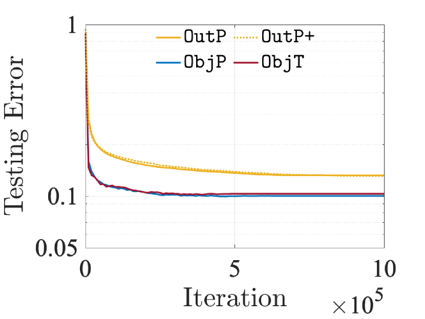
Refer to caption
Refer to caption
(a) ϵ¯=0.05¯italic-ϵ0.05\bar{\epsilon}=0.05
Refer to caption
Refer to caption
(b) ϵ¯=0.1¯italic-ϵ0.1\bar{\epsilon}=0.1
Refer to caption
Refer to caption
(c) ϵ¯=1¯italic-ϵ1\bar{\epsilon}=1
Figure 5: [MNIST] Consensus violation and testing error when ϵ¯{0.05,0.1,1}¯italic-ϵ0.050.11\bar{\epsilon}\in\{0.05,0.1,1\}.

A.11 Additional Hyperparameter Tuning for ObjP

We note that the proximity parameters δt=1/t2superscript𝛿𝑡1superscript𝑡2\delta^{t}=1/t^{2} in (9) and ηt=1/tsuperscript𝜂𝑡1𝑡\eta^{t}=1/\sqrt{t} in (8) can be scaled by multiplying a constant a(0,)𝑎0a\in(0,\infty) without affecting the convergence results, as well as the proximity parameter η^tsuperscript^𝜂𝑡\widehat{\eta}^{t} for OutP (see Theorem 4 in [10]), which is a function of 1/t1𝑡1/\sqrt{t} and numerous parameters, such as ϵ¯¯italic-ϵ\bar{\epsilon}, the Gaussian noise parameters, the numbers of data and classes, and so on.

In Figure 6, we report the testing errors of the three algorithms when their proximity parameters, namely η^t,δt,ηtsuperscript^𝜂𝑡superscript𝛿𝑡superscript𝜂𝑡\widehat{\eta}^{t},\delta^{t},\eta^{t} are multiplied by a{1,100,1000}𝑎11001000a\in\{1,100,1000\}. First, we note that OutP with a=1𝑎1a=1 as in [10] produces the best performance, which implies that the paper [10] has well calibrated the proximity parameter η^tsuperscript^𝜂𝑡\widehat{\eta}^{t}. Second, the testing errors of ObjP with a{100,1000}𝑎1001000a\in\{100,1000\} are less than those of OutP with a=1𝑎1a=1. Even for some cases, ObjP outperforms ObjT. This implies that the ObjP requires an additional hyperparameter tuning process. Lastly, we note that the testing errors of ObjT are not greatly varied according to the value of a𝑎a compared with those of ObjP. This is because the proximity of a new point zpt+1subscriptsuperscript𝑧𝑡1𝑝z^{t+1}_{p} from zptsubscriptsuperscript𝑧𝑡𝑝z^{t}_{p} in ObjP can be affected by other parameters, such as ρtsuperscript𝜌𝑡\rho^{t} in the objective function of (8) while the proximity in ObjT is controlled in the constraints. This partially shows the benefit of using ObjT.
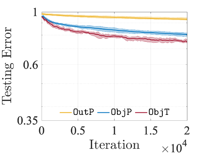
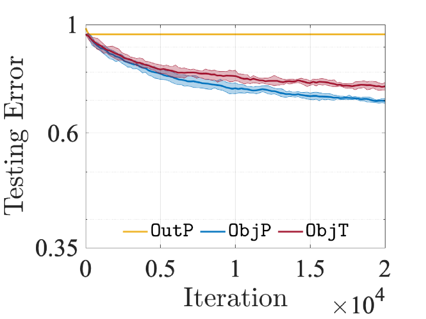
Refer to caption
Refer to caption
Refer to caption
(a) ϵ¯=0.05¯italic-ϵ0.05\bar{\epsilon}=0.05
Refer to caption
Refer to caption
Refer to caption
(b) ϵ¯=0.1¯italic-ϵ0.1\bar{\epsilon}=0.1
Refer to caption
Refer to caption
Refer to caption
(c) ϵ¯=1¯italic-ϵ1\bar{\epsilon}=1
Figure 6: [FEMNIST] Testing errors when a{1,100,1000}𝑎11001000a\in\{1,100,1000\} (top, middle, bottom).