The atomic ionization, capture, and stopping cross sections by multicharged ions satisfy the Benford law

Abstract

The applicability of the Benford law for different data sets of atomic cross sections by ion impact is studied. We find that the data sets corresponding to theoretical ionization and capture cross sections of neutral targets by multicharged ions satisfy quite well the Benford law, not only for the first digits but also within a given order of magnitude. Experimental stopping power values from the International Atomic Energy Agency data base were also scrutinized, but in this case the Benford conformity was not so satisfactory due to its small rank width. In all cases, errors, densities of prime numbers, theorems of Nigrini and Pinkham are evaluated and discussed.

I Introduction

The Benford’s Law (BL) was originally proposed by the astronomer Newcomb in 1881 Newcomb1881 and formulated  much later by Benford in 1938 Benford1938 . For a given big data set $\{\eta\}$, both man-made or from nature$,\$the Benford distribution states that the frequency of the first significant digit $\eta_{1}$ follows the following law

$$P_{\eta_{1}}^{B}=\log_{10}(1+1/\eta_{1}),$$ (1)

where $P_{\eta_{1}}^{B}$ is the Benford probability of occurring $\eta_{1}\$(not considering the number of zeros on the left of the numbers). From a mathematical point of view  Berger2011 , to identify the digits of a given real number, one can define an operator corresponding to the first $(j=1)$, second $(j=2)$ and higher digits$\ (j>2)$ of a real number $\eta$ as $\widehat{D}_{j}(\eta)=\eta_{j}$. For example if $\eta^{\ast}=0.0234$, then $\widehat{D}_{1}(\eta^{\ast})=\eta_{1}=2,\ \ \widehat{D}_{2}(\eta^{\ast})=\eta_{2}=3,\$and$\ \widehat{D}_{3}(\eta^{\ast})=\eta_{3}=4.$ The numbers formed by the first two digits is here denoted as$\ \{\eta_{1},\eta_{2}\},\ ($in our example $\{\eta_{1},\eta_{2}\}=23)$ and so on. The BL can be extended for all decimal digits: for example for the first two digits, it holds

$$P_{\{\eta_{1},\eta_{2}\}}^{B}=\log_{10}\left(1+\frac{1}{10\eta_{1}+\eta_{2}}\right).$$ (2)

Like any probability, the closure relation is normalized,

$$\sum\limits_{\eta_{1=1}}^{9}P_{\eta_{1}}^{B}=\sum\limits_{\{\eta_{1},\eta_{2}\}=10}^{99}P_{\{\eta_{1},\eta_{2}\}}^{B}=1.$$ (3)

In addition, if we are interested in the order of magnitude $M,$ we need to use the operator $\widehat{M}$, so that $\widehat{M}$ ($\eta$)$=M.$ In our example, $\widehat{M}(\eta^{\ast})=-2.$

For the first digit, $\eta_{1}\in[1,9]$, the BL states that the number $\eta_{1}=$1 appears in more than 30% of the cases, while$\ \eta_{1}=$9 in less than 5%. But the probability of appearance of the second digit,

$$P_{\eta_{2}}^{B}=\Sigma_{\eta_{1}}P_{\{\eta_{1},\eta_{2}\}}^{B},$$ (4)

varies from $P_{\eta_{2}=0}^{B}=0.1196$ to$\ P_{\eta_{2}=9}^{B}=0.0850,$ tending to the uniform distribution $P_{\eta_{m}}^{B}\rightarrow 1/10,$ as $m\rightarrow\infty.$

If we consider two-digit integer numbers, so $\{\eta_{1},\eta_{2}\}\in[10,99],$ the probability of appearing $10$ is $P_{\{\eta_{1},\eta_{2}\}=10}^{B}=0.047,$ while the one of $99$ is $P_{\{\eta_{1},\eta_{2}\}=99}^{B}=$0.004.  A list of occurring of a given digit in the first second and third positions can be found in several articles, for example in Refs.Nigrini1999 ; Nigrini2012 .

At first sight, these results are against the human perception, which would tend to assume a randomness. For a single digit,  one would guess a uniform distribution, that is, $P_{\eta_{1}}^{U}=$ 1/9 for any digit, and for two digits, $\ P_{\{\eta_{1},\eta_{2}\}}^{U}=1/90,$ and so on. This is precisely what makes interesting the BL: if the numbers are naively forged by the human mind, for example, the BL will no longer be satisfied.

It is important to note that not all data sets follow the BL, but just the ones resulting of the product of multiple independent factors that produce a probability covering several orders of magnitudes when they are plotted in a lognormal scale.

There is a huge amount of applications, like fight against tax fraud by detecting manipulation as anomalies, stock exchange data, corporate disbursements, analysis of sales figures, demographics and scientific data, etc. Nigrini1999 ; Nigrini2012 . The application of the BL crosses a huge range of disciplines, including physical sciences. Also astrophysical data like the exoplanet masses, pulsars rotation frequencies, $\gamma$-ray source fluxes and fundamental physics constants satisfy the BL Sambridge2011 ; Alexopuolos2014 ; Miraglia2021 . A complete list of articles on BL can be found in Ref. Beebe2020 .

II The atomic data sets

The values $\eta\$that we are going to scrutinize under the BL correspond to three different atomic collision data sets, namely: ionization from the subshell $nl\$of neutral atoms by impact of multicharged ions, electron capture from hydrogen to the subshell $nl$ of bare projectiles, and experimental stopping power cross sections by multicharged ions moving in gases. The numbers $n\$and $l$ denote the principal and orbital quantum numbers, respectively, of the atomic subshell. Details of these data sets will be provided in the next subsections.

II.0.1 Ionization cross section data set.

During the last years we have been calculating $nl$-ionization cross sections by multicharged ions on different neutral atoms. Calculation were carried out with the continuum distorted wave-eikonal initial state (CDW-EIS) theory. All the results were numerically performed as accurate as possible and published in Ref.Miraglia2019 .  The main aim of such calculations was the evaluation of molecular ionization cross sections within a stoichiometric model Mendez2020 .

Theoretical ionization cross sections for the following systems: antiprotons, H⁺, He²⁺, Be⁴⁺, C⁶⁺ and O⁸⁺ impinging on H, He, Li, Be, B, C, N, O, F, Ne, P, S and Ar neutral atoms for impact energies ranging from 100 to 10000 kev/amu were put together. We gather 2808 results with three significant figures covering about ten orders of magnitude. All these values were expressed in atomic units forming a data set that will be noted, for short as $\eta=I=I(nl).$ We also explore the reduced set of total ionization cross sections, $\eta=X=\Sigma_{nl}o_{nl}I(nl),\$where  $o_{nl}\$is the occupation number of the $nl$-subshell.

II.0.2 Electron capture cross section data set

We consider capture cross sections from hydrogen to the subshell $nl$ of the impinging bare ions calculated with the eikonal impulse (EI) approximation. Results for capture by H⁺ and He²⁺ projectiles to the principal quantum numbers $n=$1,2,3, and 4, and by Li${}^{3+},\$Be${}^{4+},\$B${}^{5+},$ C${}^{6+},$ N⁷⁺ and O⁸⁺ ions to the principal quantum numbers $n=$1….8 , both for orbital momentum numbers $l=0,...n-1,$ are analyzed. . In all the cases, 13 impact energies  ranging from 25 to 1220 keV/amu. were considered Jorge2015 .  We totalize a set of 3275 values which ,will be here noted, for short as $\eta=C=C(nl).\$Also the smaller set of capture cross sections to a given principal number $n,$ defined as $\eta=T=T(n)=\dsum\limits_{l}C(nl),$ will be explored.

II.0.3 Stopping power data set

We use data of experimental stopping power as stored by the web site of the International Atomic Energy Agency (IAEA) iaea .  We collected all the values corresponding to heavy ion impact on neutral gas targets. We bring together 4118 values from 52 files of the web site for the following colliding systems: H⁺, He⁺⁺, Li³⁺,  N⁹⁺, Cu²⁹⁺and  Kr³⁶⁺ impinging on  H${}_{2},$ He, N₂, O₂, Ne, Ar, Kr, and Xe. All the values were standardized to atomic units from the practical units 10^-15eVcm² and Mev cm/mg, as published in the site. Furthermore, the targets were described as they are found in nature, that is, for dimers, such as H${}_{2},$ N₂, and O₂, the results of the IAEA were multiplied by 2 because they are normalized to the number of atoms. Note that this data set represents a great challenge for the BL because it contains several experiments differing each other, specially in the intermediate and low energy regions where we may have different first digits for the same collision parameters. This set will be noted as $\eta=S$

Summarizing, the following sets will be considered

$$\eta=\left\{\begin{array}[]{ll}I=I(nl)&\text{Ionization \ cross section from the }nl\text{ level.}\\ X=\dsum\limits_{nl}I(nl),&\text{Total ionization cross section.}\\ C=C(nl)&\text{Capture\ cross section to the }nl\text{ level.}\\ T=T(n)=\dsum\limits_{l}C(nl),&\text{Total capture\ cross section to the }n\text{ level.}\\ S&\text{Stopping power cross section.}\end{array}\right.$$ (5)

These sets have no node, and they are unimodal containing only positive quantities, which make them good candidates to check if the BL is satisfied. To study any set of numerical results under the Benford scheme, one important point to bear in mind is the role of the last digit. In a numerical calculation, the last digit is generally worked through a rounding up process, while the last digit of a Benford distribution is understood via a truncation process. Therefore in our study of the BL the third (last) digit will be out of discussion.

II.1 The width and the density of points

A first requirement to inspect the BL is that the data set is expected to be evenly distributed in a logarithmic scale. It  means that the numbers, when ranked from smallest to largest, can be approximated by a linear form in a logarithmic scale, that is,

$$Log_{10}\eta\simeq a+bj,$$ (6)

where $\eta$ represents a given value of the set and$\ j$ indicates its order index in the data set, i.e. $j\in[1,J$] and $J$ is the total amount of values of the set. In all the cases, the actual values of $Log_{10}\eta\$do not fall on a straight line from start to finish; it is reasonably straight in the middle, but it is curvy in the tails. Following to Nigrini Nigrini2012 , the width $\Delta$ of a set of values can be estimated by the difference between the extremes of the linear fitting,

$$\Delta=(a+bJ)-(a+b)=b(J-1)\simeq bJ.$$ (7)

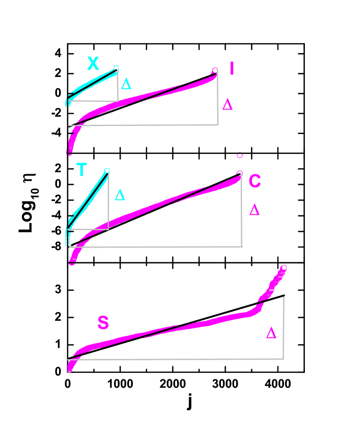
Figure 1: (Color online) Symbols, logarithm of population numbers as a function of the rank of the magnitude under study (ordered from smallest to largest). Panels (a), (b), and (c) correspond to ionization, capture and stopping power data sets, respectively. Solid line is the linear fitting as given by Eq.(6) and $\Delta$ indicates the corresponding width.

For the five sets studied in this article, the values of $\Delta$ are shown in the Table, and displayed in Figure 1. The width $\Delta$ represents the effective number of orders of magnitudes that cover the data set. The BL requires $\Delta\gg 2$ to sample the first digits at least twice. One expects the larger the width, the more robust the prediction of the BL.

For the data sets I and C, the $\Delta$ values are 5.34 and 9.31, respectively, being large enough to warranty a good spread of numbers. Instead for the stopping $S$, $\ \Delta$=2.32, being a small value which originates critical problems of borders, as we will see. A similar problem arises if we reduce the number of data. For example, by considering the total ionization cross section set $X$, the total number of data is reduced to $J=$912, with values covering just two orders of magnitude.

In order to measure this effect, we can define a new important magnitude: the density of points $\delta=J/\Delta\simeq$ $1/b$. From our experience, we find that it is required $\delta\gg$ $200$ to have a reasonable occurrence of the first digit only. For total capture cross sections to different $n-$shells, represented by the set $T$, the resulting range $\Delta\$ still covers seven orders of magnitude, but the amount of values reduces dramatically to $J=755$, given rise to  $\delta\sim 10^{2}$ which is a very small density. Hence, we are in a presence of different situations, for $X$, $\Delta$ is substantially reduced, while for $T$, $\delta$ is too small. Results are displayed in the Table for all the cases.

II.2 The degree of ”Benfordness”

At this stage one should develop a tool to quantify how good the data conform the BL, or in other words, to quantify the ”Benfordness” of a  given data set under study. A traditional approach is to use the chi-squared statistic. However, this test is not useful for very large data sets since for a large value of $J,$ the calculated chi-square will generally be higher than the critical value, leading us to conclude that the data set does not conform the BL Nigrini2012 . A specific method to measure the Benfordness of the data is the mean absolute deviation (MAD) test. For the first digit the MAD test is defined in percentages as Nigrini2012

$$\varepsilon_{1}^{B}=\frac{1}{9}\sum\limits_{\eta_{1}=1}^{9}\left|P_{\eta_{1}}-P_{\eta_{1}}^{B}\right|\times 100,$$ (8)

where $P_{\eta_{1}}$ is the actual frequency of the first digit of the magnitude $\eta$ and $P_{\eta_{1}}^{B}$ is the corresponding prediction of the BL, as given by Eq.(1). Nigrini Nigrini2012 published some guidelines, based on his personal experience, to qualify the Benfordness according with the value of $\varepsilon_{1}^{B}$ as it follows

$$\left\{\begin{array}[]{ll}0.0\%\lesssim\varepsilon_{1}^{B}\lesssim 0.6\%,&\text{{close conformity,}}\\ 0.6\%\lesssim\varepsilon_{1}^{B}\lesssim 1.2\%,&\text{{acceptable conformity,}}\\ 1.2\%\lesssim\varepsilon_{1}^{B}\lesssim 1.5\%,&\text{{marginal conformity.}}\end{array}\right..$$ (9)

If we rule out the rigor of the accountancy to detect frauds, we would be very satisfied if we can comply with these figures. Just for comparison we could define equivalently a MAD error corresponding to the uniform distribution

$$\varepsilon_{1}^{U}=\frac{1}{9}\sum\limits_{\eta_{1}=1}^{9}\left|P_{\eta_{1}}-P_{\eta_{1}}^{U}\right|\times 100,$$ (10)

where $P_{\eta_{1}}^{U}=$1/9 is the uniform (random) prediction.  One would expect that the ratio

$$\rho_{1}^{B}=\frac{\varepsilon_{1}^{B}}{\varepsilon_{1}^{U}}$$ (11)

to be $\rho_{1}^{B}\ll 1$ to indicate that we are in a presence of a Benford distribution.

As far as the first digit is concerned there is an interesting alternative test, introduced by Nigrini Nigrini2012 to diagnose a Benford distribution. Consider an any-digit set of a given magnitude $\eta=\{\eta_{1},\eta_{2},...\}\$ and calculate

$$N_{\mu_{1}}=\frac{\sum\limits_{\eta}\{\eta_{1},\eta_{2},...\}\delta_{\eta_{1},\mu_{1}}}{\sum\limits_{\eta}\{\eta_{1},\eta_{2},...\}},$$ (12)

with $\mu_{1}\in[1,9].\$The second theorem of Nigrini Nigrini2012 states that the Benford distribution produces $N_{\mu_{1}}\rightarrow N_{\mu_{1}}^{B}=1/9.$ Therefore, this is another independent strategy to check whether the set under study satisfies the BL. This new parameter allows us to introduces an equivalent Nigrini MAD error $\varepsilon_{1}^{N}$ to assert the Benfordness of the set under study, as

$$\varepsilon_{1}^{N}=\frac{1}{9}\sum\limits_{\eta_{1}=1}^{9}\left|N_{\eta_{1}}-N_{\eta_{1}}^{B}\right|\times 100.$$ (13)

The analysis of the second digit demands a more fine attention because $P_{\eta_{2}}^{B}$ is close to randomness $P_{\eta_{2}}^{U}=$1/10 and a differentiation is required. To this end, we find convenient to define the ratio of MAD errors

$$\rho_{2}^{B}=\frac{\varepsilon_{2}^{B}}{\varepsilon_{2}^{U}}=\frac{\frac{1}{10}\sum\limits_{\eta_{2}=0}^{9}\left|P_{\eta_{2}}-P_{\eta_{2}}^{B}\right|}{\frac{1}{10}\sum\limits_{\eta_{2}=0}^{9}\left|P_{\eta_{2}}-P_{\eta_{2}}^{B}\right|},$$ (14)

which gives an indication of the goodness of the second digit to conform the Benford distribution. In similar fashion with $\rho_{1}^{B},$ we can state:  if $\rho_{2}^{B}>1,$ the second digit of the set is ruled by randomness, while $\rho_{2}^{B}<1$ indicates that the set is ruled by Benford. Then, the smaller $\rho_{2}^{B},$ the closer to the Benford distribution. Values of $\varepsilon_{1}^{B},\ \varepsilon_{1}^{U},\ \varepsilon_{1}^{N},$ $\rho_{2}^{B}~{}$and $\ \rho_{2}^{B},$ for all the sets are shown in the Table.

III Results

III.0.1 Ionization cross sections

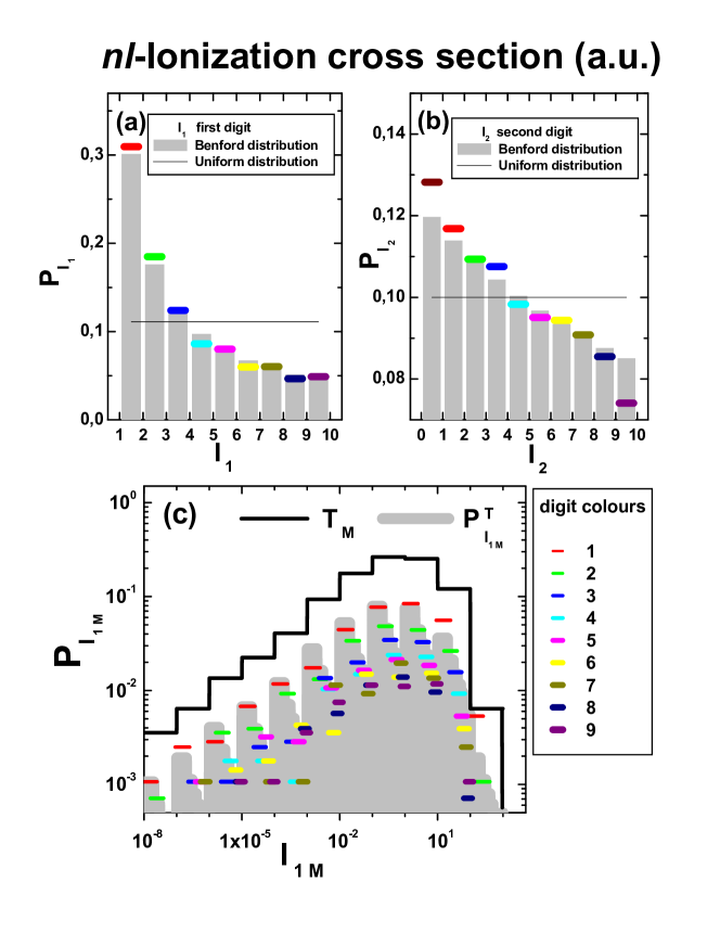
Figure 2: (Color online) Color symbols are the frequencies of (a) the first digits and (b) second digits from the data set of $nl$-ionization cross sections. The light grey histogram represents the Bendford predictions, and the horizontal black solid line in black denotes the uniform distribution. (c) Color symbols are the distribution of the first digits within each decade: $I_{1M}=I_{1}\times 10^{M}$. The solid line histogram represents the top function as defined in Eq.(15). The light grey histogram represents the Benfordization estimation given by Eq.(16).

We start analyzing the probability of occurring the first figure of  $nl$-ionization data, denoted as $P_{I_{1}}$ in Fig. 2(a). We compare $P_{I_{1}}$ with the Benford prediction $P_{I_{1}}^{B}$ given by Eq.(1) and indicated as a histogram in light grey. The agreement is very good and in consequence the MAD error is very small,$\ \varepsilon_{1}^{B}=0.52\%$ (see Table) which means that, according to (9), we can certify the agreement as close conformity. The second theorem of Nigrini produces a very similar error, $\varepsilon_{1}^{N}=0.62\%$, which stands as an alternative criterion to assess the Benfordness using the same categorization of (9).

We can go further by studying the probability to have a given second digit $I_{2}\in[0,9],$ denoted as $P_{I_{2}},$ shown in Fig 2(b). Again, the agreement with the Benford prediction is quite good.

To get deeper the analysis, we should proceed to calculate the two-digit probability $P_{\{I_{1},I_{2}\}}.$ But instead, we prefer to introduce a novel criterion based on the prediction of the density of two-digit prime numbers $\pi_{2},$ which is a very sensitive and sharp value, reduced to the range [10-99]. This represents a new parameter that subvert human thinking. One would tend to think that $\pi_{2}$ equals that of the uniform distribution, $\pi_{2}^{U}=21/90=0.233$. But this is not true for a Benford distribution. By using Eq.(2) one can easily obtain $\pi_{2}^{B}=0.266$. Our {$I_{1},I_{2}$}   data produce $\pi_{2}=0.262\$in close agreement with the BL prediction. Therefore, we can conclude categorically that our $nl$-ionization cross section data set satisfies very well the BL.

We are also interested in studying the BL within a given order of magnitude. In Fig. 2(c) we plot the data corresponding to the occurrence of a single digit within a given order of magnitude, that is $\ I_{1M}=I_{1}\times 10^{M}$ .  Even though the results for $\ I_{1M}$ spread along 9 orders of magnitudes, from $10^{-8}$ to $10^{0}$, it becomes evident that the BL still applies within each order of magnitude. To visualize this behavior more clearly, we first define a top function for a given order of magnitude $M$ as

$$T_{M}=\sum\nolimits_{I_{1}}P_{I_{1M}},$$ (15)

which plays the role of a closure relation within the range of magnitude $M$.  Hence the probability $P_{I_{1M}}$ can be estimated by simply Benfordizing the top function, i.e.

$$P_{I_{1M}}^{T}\simeq\log_{10}(1+1/I_{1})T_{M}\ ,$$ (16)

which is plotted in in Fig. 2(c). From this figure one can observe that $P_{I_{1}M}^{T}$ guides quite well the data values, indicating that all the substantial information can be reduced to $M$ values of the top function $T_{M}.$

On the other hand, the total cross section set $X$ is another matter because it is spread in a little more than two orders of magnitude (see the Table). But we can still verify that $X$ follows the first-digit BL with an error of $\varepsilon_{1}^{B}=1.2\%,$ which means that we can certify the agreement as acceptable conformity.

III.0.2 Capture cross sections

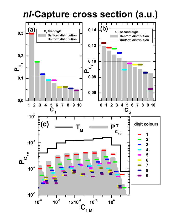
Figure 3: (color on line) Similar to Fig. 2 for $nl$-capture cross sections.

Fig. 3(a) shows the probability of occurring the first figure of the $nl$-capture cross section data set$\ P_{C_{1}}$ which is compared with the Benford prediction given by Eq.(1). The agreement is good and  the MAD error is small, $\ \varepsilon_{1}^{B}=0.57\%$ , complying with the close conformity according with the categorization (9). The second digit does not look so well but it is better than the uniform distribution, with $\rho_{2}^{B}$¡1 (see the Table). Moreover, the  distribution along ten orders of magnitudes follows reasonably well the ”Benfordization” of the top probability shown in light grey in Fig. 3(c).

Instead for the capture cross section to the $n-$state data set $T$,  the first digit probability degrades to acceptable conformity (see Table), while its second digit does not present any bias to Benford nor to uniform because $\rho_{2}^{B}=1.03.$

III.0.3 Stopping power cross sections

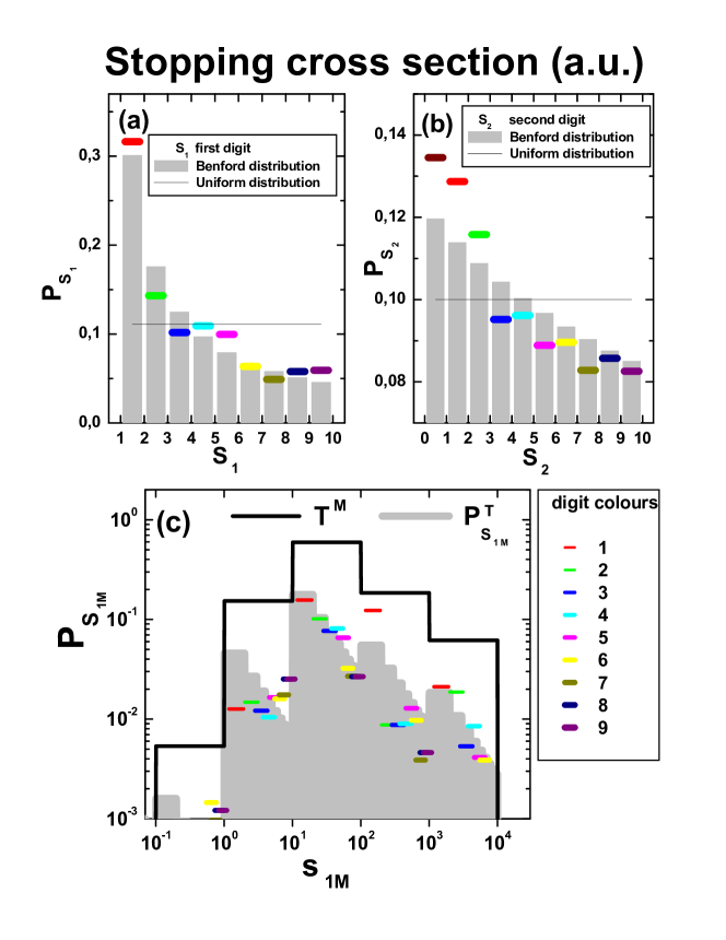
Figure 4: (color on line) Similar to Fig. 2 for stopping power cross sections from IAEA data base.

This is a case in which not only the width $\Delta\$is small, but also we are dealing with a large variety of experimental data from different laboratories. As shown in Fig. 4(a) the first digit probability $P_{S_{1}}$ resembles to the histogram of Benford, but the MAD error is high, $\varepsilon_{1}^{B}=1.52\%,$  which hardly qualifies within the category of marginal conformity, as classified in (9). Nonetheless, the shape is definitively more close to the BL than to the uniform distribution ($\varepsilon_{1}^{U}=5.3\%$ ). The second digit distribution (Fig. 4(b)) does not differ a lot from the one of Benford because $\rho_{2}^{B}=0.46<1$.  On the contrary, the magnitude $P_{S_{1M}}$ does not follows the logarithmic structure within each order of magnitude as in the previous cases, as shown in Fig. 4(c).

III.1 Two numerical experiences

III.1.1 Testing the universal scaling of Pinkham.

One of the most extraordinary property of the BL is its scale invariance, to the point that it is possible to obtain it mathematically by just invoking this property, as discovered by Pinkham Pinkham1961 . From the physics point of view, this is evident because BL should be independent on the units that we use. Ideally, as the Benford distribution is based on the logarithmic function, any multiplicative factor will just shift the distribution keeping intact the occurrences of the digits. This is the case if we have a big width $\Delta$. However, there is a limitation when the width $\Delta$ is small, like in the case of the stopping power cross sections. This limitation surfaces clearly due to the border effects in a limited width. As $\Delta$ is small, the reduction or enhancement of the probabilities corresponding to some digits will be transferred to other digits when a different unit is used.

In our analysis, we use atomic units for ionization cross sections, but we could have used any other magnitude, that is cm² or whatever we choose. For example, if we transform the set of $nl-$ionization values  $I$ in cm² we need to multiply by 2.800$\times 10^{-17}$. This change of scale produces $\varepsilon_{1}^{B}=0.43$% which lightly differs from from the error 0.52% obtained with atomic units, i.e., a difference of 0.1%. It is important to note that the order of magnitude of the units is irrelevant since it just replicate the same digits. But if we built the set of stopping power cross sections in  10^-15eVcm², we should multiply the set by 1.213, finding $\varepsilon_{1}^{B}=1.9$%  which is substantially greater than the error $1.5\%$ obtained when expressed in atomic units (that is a difference of 0.4%). This difference is a consequence of the border effects due to the small width $\Delta$. Note that in units of 10^-15eVcm${}^{2},$ the stopping power set no longer classify as marginal conformity.

III.1.2 The whole data set

We essay a daring experience by gathering all the data, $nl$-ionization, $nl$-capture and stopping power cross sections (all expressed in atomic units). We totalize 10201 values in only one numerical universe. We found that this big set of values satisfies reasonable well the BL with $\varepsilon_{1}^{B}=0.67$% and $\rho_{2}^{B}=0.33$%. However it does not represent an overall improvement of the BL conformity. The explanation is related to the stopping power set which adds 4118 values in a short width, introducing a high density that disturbs the required even distribution in the logarithmic scale. This behaviour demonstrate that a large number of values not necessarily improves the Benford distribution, but the stability of the density of points.

IV Conclusion

We have studied three different sets of atomic data with the BL, having three different qualifications, according to the Nigrini scheme: close, acceptable and marginal conformities corresponding to the $nl$-ionization, $nl$-capture and experimental stopping power cross sections of multicharged ions on gases, respectively. This findings allows us to conclude that any atomic-collision data set having the appropriate width $\Delta\$and density of points $\delta$ will satisfy the Bendford distribution. Furthermore, the parameters here introduced to quantify the degree of conformity of the BL, like the MAD errors, could be used as a useful tools to check the quality of any atomic data set and detect systematic experimental errors or theoretical biases.

The authors acknowledge the financial support from the following institutions of Argentina: Consejo Nacional de Investigaciones Científicas y Técnicas (CONICET), Agencia Nacional de Promoción Científica y Técnológica (ANPCyT), and Universidad of Buenos Aires.

V Bibliography.

Table 1: MAD errors, ratios, widths and densities as defined in the tex for the data sets given in (5)

$\eta$	$I$	$X$	$C$	$T$	$S$
J	2808	925	3275	755	4118
$\Delta$	5.34	2.78	9.31	6.96	2.32
$\delta$	413	331	351	108	1778
$\varepsilon^{B}_{1}$ (%)	0.52	1.02	0.46	0.76	1.52
$\varepsilon^{U}_{1}$(%)	6.33	5.11	5.75	5.92	5.27
$\varepsilon^{N}_{1}$(%)	0.63	1.22	0.73	1.08	1.72
$\rho^{B}_{1}$	0.08	0.20	0.08	1.27	0.29
$\rho^{B}_{2}$	0.27	0.56	0.47	1.03	0.46
$\pi_{2}$	0.262	0.270	0.257	0.244	0.268

References

- (1) S. Newcomb, Note on the frequency of use of the different digits in natural numbers, Am. J. of Math., 9, 201-205 (1881)
- (2) F. Benford, The law of anomalous numbers. Proc. Amer Philos. Soc., 78, 551–572 (1938)
- (3) A. Berger and T. P. Hill, A basic theory of Benford´s Law, Probability Survey 8, 1-126 (2011)
- (4) M. J. Nigrini, I´ve got your number: How a mathematical phenomenon can help CPAs uncover fraud and other irregularities. Journal of Accountancy, 187(5), 79–83 (1999)
- (5) M. J. Nigrini, Benford´s law: applications for forensic accounting, auditing, and fraud detection (The Wiley Corporate F&A series) ISBN 978-1-118-15285-0 (2012)
- (6) M. Sambridge, H. Tkalčić, and A. Jackson, Benford´s Law in the natural sciences. Geophys. Res Lett 37, L22301 (2010)
- (7) T. Alexopoulos and S. Leontsinis, Benford´s Law in Astronomy .J. Astrophys. Astr. 35, 639–648 (2014)
- (8) J. E. Miraglia and M. D. Melita, On the applicability of Benford law to exoplanetary data, to be published.
- (9) N. H. F. Beebe, A bibliography of publications about Bendford´s Law, Heaps´ law, Heps ´law and Zipf´s law, https://www.math.utah.edu/beebe/.
- (10) J. E. Miraglia, arXiv:1909.13682v2 [physics.atom-ph]) (2019).
- (11) A. M. P. Mendez, C. C. Montanari, J. Phys B: At. Mol. Opt. Phys. 53, 055201 (2020)
- (12) A. Jorge, C. Illescas, J. E. Miraglia, and M. S. Gravielle, J. Phys. B 48, 235201 (2015)
- (13) International Atomic Energy Agency. Stopping Power of Matter for Ions, Graphs, Data, Comments and Programs, https://www-nds.iaea.org/stopping/
- (14) R. S. Pinkham, On the distribution of first significant digits, Ann. Math. Statist. 32, 1223-1230 (1961)