RNN with Particle Flow for Probabilistic Spatio-temporal Forecasting

Abstract

Spatio-temporal forecasting has numerous applications in analyzing wireless, traffic, and financial networks. Many classical statistical models often fall short in handling the complexity and high non-linearity present in time-series data. Recent advances in deep learning allow for better modelling of spatial and temporal dependencies. While most of these models focus on obtaining accurate point forecasts, they do not characterize the prediction uncertainty. In this work, we consider the time-series data as a random realization from a nonlinear state-space model and target Bayesian inference of the hidden states for probabilistic forecasting. We use particle flow as the tool for approximating the posterior distribution of the states, as it is shown to be highly effective in complex, high-dimensional settings. Thorough experimentation on several real world time-series datasets demonstrates that our approach provides better characterization of uncertainty while maintaining comparable accuracy to the state-of-the-art point forecasting methods.

1 Introduction

Spatio-temporal forecasting has many applications in intelligent traffic management, computational biology and finance, wireless networks and demand forecasting. Inspired by the surge of novel learning methods for graph structured data, many deep learning based spatio-temporal forecasting techniques have been proposed recently (Li et al., 2018; Bai et al., 2020). In addition to the temporal patterns present in the data, these approaches can effectively learn and exploit spatial relationships among the time-series using various Graph Neural Networks (GNNs) (Defferrard et al., 2016; Kipf & Welling, 2017). Recent works establish that graph-based spatio-temporal models outperform the graph-agnostic baselines (Li et al., 2018; Wu et al., 2020). In spite of their accuracy in providing point forecasts, these models have a serious drawback as they cannot gauge the uncertainty in their predictions. When decisions are made based on forecasts, the availability of a confidence or prediction interval can be vital.

There are numerous probabilistic forecasting techniques for multivariate time-series, for example, DeepAR (Salinas et al., 2020), DeepState (Rangapuram et al., 2018), DeepFactors (Wang et al., 2019), and the normalizing flow-based algorithms in (Kurle et al., 2020; Rasul et al., 2021). Although these algorithms can characterize uncertainty via confidence intervals, they are not designed to incorporate side-knowledge provided in the form of a graph.

In this work, we model multivariate time-series as random realizations from a nonlinear state-space model, and target Bayesian inference of the hidden states for probabilistic forecasting. The general framework we propose can be applied to univariate or multivariate forecasting problems, can incorporate additional covariates, can process an observed graph, and can be combined with data-adaptive graph learning procedures. For the concrete example algorithm deployed in experiments, we build the dynamics of the state-space model using graph convolutional recurrent architectures. We develop an inference procedure that employs particle flow, an alternative to particle filters, that can conduct more effective inference for high-dimensional states.

The novel contributions in this paper are as follows:
1) we propose a graph-aware stochastic recurrent network architecture and inference procedure that combine graph convolutional learning, a probabilistic state-space model, and particle flow;
2) we demonstrate via experiments on graph-based traffic datasets that a specific instantiation of the proposed framework can provide point forecasts that are as accurate as the state-of-the-art deep learning based spatio-temporal models. The prediction error is also comparable to the existing deep learning based techniques for benchmark non-graph multivariate time-series datasets;
3) we show that the proposed method provides a superior characterization of the prediction uncertainty compared to existing probabilistic multivariate time-series forecasting methods, both for datasets where a graph is available and for settings where no graph is available.

2 Related Work

Our work is related to (i) multivariate and spatio-temporal forecasting using deep learning and graph neural networks; (ii) stochastic/probabilistic modelling, prediction and forecasting for multivariate time-series; and (iii) neural (ordinary) differential equations. Recently, neural network-based techniques have started to offer the best predictive performance for multivariate time-series prediction (Bao et al., 2017; Qin et al., 2017; Lai et al., 2018; Guo & Lin, 2018; Chang et al., 2018; Li et al., 2019; Sen et al., 2019; Oreshkin et al., 2020; Smyl, 2020). In some settings, a graph is available that specifies spatial or causal relationships between the time-series. Numerous algorithms have been proposed that combine GNNs with temporal neural network architectures (Li et al., 2018; Yu et al., 2018; Huang et al., 2019; Bai et al., 2019; Chen et al., 2019a; Guo et al., 2019; Wu et al., 2019; Yu et al., 2019; Zhao et al., 2019; Bai et al., 2020; Huang et al., 2020; Park et al., 2020; Shi et al., 2020; Song et al., 2020; Xu et al., 2020; Wu et al., 2020; Zheng et al., 2020; Oreshkin et al., 2021). Algorithms that take into account the graph provide superior forecasts, if the graph is accurate and the indicated relationships have predictive power. However, none of these algorithms is capable of characterizing the uncertainty of the provided predictions; all are constructed as deterministic algorithms.

Recently, powerful multivariate forecasting algorithms that are capable of providing uncertainty characterization have been proposed. These include DeepAR (Salinas et al., 2020), DeepState (Rangapuram et al., 2018), the Multi-horizon Quantile RNN (MQRNN) (Wen et al., 2017), the Gaussian copula process approach of (Salinas et al., 2019), and DeepFactors (Wang et al., 2019). Normalizing flow has also been combined with temporal NN architectures (Kumar et al., 2019; de Bézenac et al., 2020; Gammelli & Rodrigues, 2020; Rasul et al., 2021). Various flavours of stochastic recurrent networks have also been introduced (Boulanger-Lewandowski et al., 2012; Bayer & Osendorfer, 2014; Chung et al., 2015; Fraccaro et al., 2016, 2017; Karl et al., 2016; Mattos et al., 2016; Doerr et al., 2018). In most cases, variational inference is applied to learn model parameters, although sequential Monte Carlo has also been employed (Gu et al., 2015; Le et al., 2017; Maddison et al., 2017; Zheng et al., 2017; Karkus et al., 2018; Naesseth et al., 2018; Ma et al., 2020). These are related to methods that determine the parameters of sequential Monte Carlo models via optimizing Monte Carlo objectives (Maddison et al., 2017; Naesseth et al., 2018; Le et al., 2017).

Our proposed method is different from this body of work in two important ways. First, we design a probabilistic state-space modeling framework that can incorporate information about predictive relationships that is provided in the form of a graph. Second, our inference procedure employs particle flow, which avoids the need for some of the approximations required by a variational inference framework and is much better suited to high-dimensional states than particle filtering. Our particle flow method has connections to normalizing flows (Kobyzev et al., 2020) and to neural ordinary differential equations (Chen et al., 2018, 2019b). In particular, Chen et al. (2019b) address a Bayesian inference task by solving a differential equation to transport particles from the prior to the posterior distribution. However, such flow-based methods were first introduced by Daum & Huang (2007) in the sequential inference research literature.

3 Problem Statement

We address the task of discrete-time multivariate time-series prediction, with the goal of forecasting multiple time-steps ahead. We assume that there is access to a historical dataset for training, but after training the model must perform prediction based on a limited window of historical data. Let $\mathbf{y}_{t}\in\mathbb{R}^{N\times 1}$ be an observed multivariate signal at time $t$ and $\mathbf{Z}_{t}\in\mathbb{R}^{N\times d_{z}}$ be an associated set of covariates. The $i$-th element of $\mathbf{y}_{t}$ is the observation associated with time-series $i$ at time-step $t$.

We also allow for the possibility that there is access to a graph $\mathcal{G}=(\mathcal{V},\mathcal{E})$, where $\mathcal{V}$ is the set of $N$ nodes and $\mathcal{E}\subset\mathcal{V}\times\mathcal{V}$ denotes the set of edges. In this case, each node corresponds to one time-series. The edges indicate probable predictive relationships between the variables, i.e., the presence of an edge $(i,j)$ suggests that the historical data for time-series $i$ is likely to be useful in predicting time-series $j$. The graph may be directed or undirected.

The goal is to construct a model that is capable of processing, for some time offset $t_{0}$, the data $\mathbf{Y}_{t_{0}+1:t_{0}+P}$, $\mathbf{Z}_{t_{0}+1:t_{0}+P+Q}$ and (possibly) the graph $\mathcal{G}$, to estimate $\mathbf{Y}_{t_{0}+P+1:t_{0}+P+Q}$. The prediction algorithm should produce both point estimates and prediction intervals. The performance metrics for the point estimates include mean absolute error (MAE), mean absolute percentage error (MAPE), and root mean squared error (RMSE). For the prediction intervals, the performance metrics include the Continuous Ranked Probability Score (CRPS) (Gneiting & Raftery, 2007), and the P10, P50, and P90 Quantile Losses (QL) (Salinas et al., 2020; Wang et al., 2019). Expressions for these performance metrics are provided in the supplementary material.

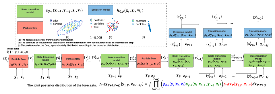
Figure 1: Probabilistic forecasting from the state-space model using particle flow. Migration of particles from a 2-d Gaussian prior to a 2-d Gaussian posterior distribution is illustrated as an example.

4 Background: Particle Flow

Particle flow is an alternative to particle filtering for Bayesian filtering (and prediction) in a state-space model. The filtering task is to approximate the posterior distribution of the state trajectory $p_{\Theta}(\mathbf{x}_{t}|\mathbf{y}_{1:t})$ recursively, where $\mathbf{x}_{t}$ denotes the state at time $t$ and $\mathbf{y}_{1:t}$ are observations from times $1$ to $t$. A particle filter (Gordon et al., 1993; Doucet & Johansen, 2009) maintains a population of $N_{p}$ samples (particles) and associated weights $\{\mathbf{x}_{t}^{j},w_{t}^{j}\}_{j=1}^{N_{p}}$ that it uses to approximate the marginal posterior distribution of $\mathbf{x}_{t}$:

$$p_{\Theta}(\mathbf{x}_{t}|\mathbf{y}_{1:t})\approx\frac{1}{N_{p}}\sum_{j=1}^{N_{p}}w^{(j)}_{t}\delta(\mathbf{x}_{t}-\mathbf{x}_{t}^{j})\,.$$ (1)

Here, $\delta(\cdot)$ denotes the Dirac-delta function. Particles are propagated by the application of importance sampling using a proposal distribution; the weights are updated accordingly. When the disparity in the weights becomes too great, resampling is applied, with particles being sampled proportionally to their weights and the weights being reset to 1. Constructing well-matched proposal distributions to the posterior distribution in high-dimensional state-spaces is extremely challenging. A mismatch between the proposal and the posterior leads to weight degeneracy after resampling, which results in poor performance of particle filters in high-dimensional problems (Bengtsson et al., 2008; Snyder et al., 2008; Beskos et al., 2014). Instead of sampling, particle flow filters offer a significantly better solution by transporting particles continuously from the prior to the posterior (Daum & Huang, 2007; Ding & Coates, 2012).

For a given time step $t$, particle flow algorithms solve differential equations to gradually migrate particles from the predictive distribution so that they represent the posterior distribution after the flow. A particle flow can be modelled by a background stochastic process $\eta_{\lambda}$ in a pseudo-time interval $\lambda\in[0,1]$, such that the distribution of $\eta_{0}$ is the predictive distribution $p_{\Theta}(\mathbf{x}_{t}|\mathbf{y}_{1:t-1})$ and the distribution of $\eta_{1}$ is the posterior distribution $p_{\Theta}(\mathbf{x}_{t}|\mathbf{y}_{1:t})$.

One approach (Daum et al., 2010), is to use an ordinary differential equation (ODE) with zero diffusion to govern the flow of $\eta_{\lambda}$:

$$\vspace{-0.1cm}\dfrac{d\eta_{\lambda}}{d\lambda}=\varphi(\eta_{\lambda},\lambda)\,\,.$$ (2)

For linear Gaussian state-space models, the flow can be expressed in the form:

$$\vspace{-0.15cm}\varphi(\eta_{\lambda},\lambda)=A(\lambda)\eta_{\lambda}+b(\lambda)\,\,,\vspace{-0.05cm}$$ (3)

and we can derive analytical expressions for $A(\lambda)$ and $b(\lambda)$ (see supplementary material for details). For non-linear and non-Gaussian models, we employ Gaussian approximations and repeated local linearizations.

5 Methodology

5.1 State-space model

We postulate that $\mathbf{y}_{t}\in\mathbb{R}^{N\times 1}$ is the observation from a Markovian state space model with hidden state $\mathbf{X}_{t}\in\mathbb{R}^{N\times d_{x}}$. We denote by $\mathbf{x}_{t}$ and $\mathbf{z}_{t}$ the vectorizations of $\mathbf{X}_{t}$ and $\mathbf{Z}_{t}$, respectively. The state space model is:

$$\mathbf{x}_{1} \sim p_{1}(\cdot,\mathbf{z}_{1},\rho)\,,$$ (4)

$$\mathbf{x}_{t} =g_{\mathcal{G},\psi}(\mathbf{x}_{t-1},\mathbf{y}_{t-1},\mathbf{z}_{t},\mathbf{v}_{t}),\text{ for }t>1\,,$$ (5)

$$\mathbf{y}_{t} =h_{\mathcal{G},\phi}(\mathbf{x}_{t},\mathbf{z}_{t},\mathbf{w}_{t}),\text{ for }t\geqslant 1\,.$$ (6)

Here $\mathbf{v}_{t}\sim p_{v}(\cdot|\mathbf{x}_{t-1},\sigma)$ and $\mathbf{w}_{t}\sim p_{w}(\cdot|\mathbf{x}_{t},\gamma)$ are the noises in the dynamic and measurement models respectively. $\rho$, $\sigma$ and $\gamma$ are the parameters of the distribution of the initial state $\mathbf{x}_{1}$, process noise $\mathbf{v}_{t}$ and measurement noise $\mathbf{w}_{t}$ respectively. $g$ and $h$ denote the state transition and measurement functions, possibly linear or nonlinear, with parameters $\psi$ and $\phi$ respectively. The subscript $\mathcal{G}$ in $g$ and $h$ indicates that the functions are potentially dependent on the graph topology. We assume that $h_{\mathcal{G},\phi}(\mathbf{x}_{t},\mathbf{z}_{t},0)$ is a $\mathcal{C}^{1}$ function in $\mathbf{x}_{t}$, i.e., $h_{\mathcal{G},\phi}(\mathbf{x}_{t},\mathbf{z}_{t},\mathbf{0})$ is a differentiable function whose first derivative w.r.t. $\mathbf{x}_{t}$ is continuous. The complete set of the unknown parameters is formed as: $\Theta=\{\rho,\psi,\sigma,\phi,\gamma\}$. Figure 2 depicts the graphical model relating the observed variables ($\mathbf{y}_{t}$ and $\mathbf{z}_{t}$) to the latent variables ($v_{t}$, $w_{t}$) and the graph ($\mathcal{G}$).

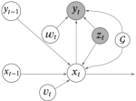
Figure 2: The graphical model representation of the state-space model in Section 5.1

With the proposed formulation, we can modify recurrent graph convolutional architectures when designing the function $g$. When a meaningful graph is available, such architectures significantly outperform models that ignore the graph. For example, we conduct experiments by incorporating into our general model the Adaptive Graph Convolutional Gated Recurrent Units (AGCGRU) presented in (Bai et al., 2020). The AGCGRU combines (i) a module that adapts the provided graph based on observed data, (ii) graph convolution to capture spatial relations, and (iii) a GRU to capture evolution in time. The example model used for experiments thus employs an $L$-layer AGCRU with additive Gaussian noise to model the system dynamics $g$:

$$\mathbf{x}_{t} =AGCGRU_{\mathcal{G},\psi}^{(L)}(\mathbf{x}_{t-1},\mathbf{y}_{t-1},\mathbf{z}_{t})+\mathbf{v}_{t}\,,$$ (7)

$$\mathbf{y}_{t} =\mathbf{W}_{\phi}\mathbf{x}_{t}+\mathbf{w}_{t}\,.$$ (8)

In this model, we have $p_{v}(\mathbf{v}_{t})=\mathcal{N}(\mathbf{0},\sigma^{2}\mathbf{I})$, i.e., the latent variables for the dynamics are independent. The initial state distribution is also chosen to be isotropic Gaussian, i.e., $p_{1}(\mathbf{x}_{1},\mathbf{z}_{1},\rho)=\mathcal{N}(\mathbf{0},\rho^{2}\mathbf{I})$. The parameters $\rho$ and $\sigma$ are learnable variance parameters. The observation model $g$ incorporates a linear projection matrix $\mathbf{W}_{\phi}$. The latent variable $\bm{w}_{t}$ for the emission model is modelled as Gaussian with variance dependent on $\mathbf{x}_{t}$ via a learnable softplus function:

$$p_{w}(\mathbf{w}_{t}|\mathbf{x}_{t})=\mathcal{N}\Big{(}\mathbf{0},\text{diag}\big{(}\text{softplus}(\bm{C}_{\gamma}\bm{x}_{t})\big{)}^{2}\Big{)}\,.$$ (9)

5.2 Inference

We assume that a dataset $\mathcal{D}_{trn}$ is available for training. Although this data may be derived from a single time-series, because our task is to predict $\mathbf{y}_{t_{0}+P+1:t_{0}+P+Q}$ using a limited historical window $\mathbf{y}_{t_{0}+1:t_{0}+P}$, we splice the time-series and thus construct multiple training examples, denoted by $(\mathbf{y}_{1:P}^{(m)},\mathbf{y}_{P+1:P+Q}^{(m)})$. In the training set, all of these observations are available; in the test set $\mathbf{y}_{P+1:P+Q}$ are not. In addition, the associated covariates $\mathbf{z}_{1:P+Q}$ are known for both training and test sets.

Inference involves an iterative process. We randomly initialize the parameters of the model to obtain $\Theta_{0}$. Subsequently, at the $k$-th iteration of the algorithm (processing the $k$-th training batch), we first draw samples $\{\mathbf{y}^{i}_{P+1:P+Q}\}_{i=1}^{N_{p}}$ from the distribution $p_{\Theta_{k-1}}(\mathbf{y}_{P+1:P+Q}|\mathbf{y}_{1:P},\mathbf{z}_{1:P+Q})$. With this set of samples, we can subsequently apply a gradient descent procedure to obtain the updated model parameters $\Theta_{k}$. We discuss each of these steps in turn as follows.

5.2.1 Sampling

In a Bayesian setting with known model parameters $\Theta=\Theta_{k-1}$, we would aim to form a prediction by approximating the posterior distribution of the forecasts, i.e., $p_{\Theta}(\mathbf{y}_{P+1:P+Q}|\mathbf{y}_{1:P})$. (For conciseness we drop the time-offset $t_{0}$).

$$p_{\Theta}(\mathbf{y}_{P+1:P+Q}|\mathbf{y}_{1:P},\mathbf{z}_{1:P+Q})=\int\prod_{t=P+1}^{P+Q}\Big{(}p_{\phi,\gamma}(\mathbf{y}_{t}|\mathbf{x}_{t},\mathbf{z}_{t})\,$$

$$p_{\psi,\sigma}(\mathbf{x}_{t}|\mathbf{x}_{t-1},\mathbf{y}_{t-1},\mathbf{z}_{t})\Big{)}p_{\Theta}(\mathbf{x}_{P}|\mathbf{y}_{1:P},\mathbf{z}_{1:P})d\mathbf{x}_{P:P+Q}\,.$$ (10)

Since the integral in eq. (10) is analytically intractable for a general nonlinear state-space model, we take a Monte Carlo approach as follows:

Step 1: For $1\leqslant t\leqslant P$, we apply a particle flow algorithm (details in Sec. 4) with $N_{p}$ particles for the state-space model specified by eqs. (4), (5) and (6) to recursively approximate the posterior distribution of the states:

$$p_{\Theta}(\mathbf{x}_{t}|\mathbf{y}_{1:t},\mathbf{z}_{1:t})\approx\frac{1}{N_{p}}\sum_{j=1}^{N_{p}}\delta(\mathbf{x}_{t}-\mathbf{x}_{t}^{i})\,.\vspace{-0.2cm}$$ (11)

Here $\{\mathbf{x}_{t}^{j}\}_{j=1}^{N_{p}}$ are approximately distributed according to the posterior distribution of $\mathbf{x}_{t}$. The generation of each sample $\mathbf{x}_{t}^{j}$ involves an associated sampling of the latent variables $\mathbf{v}_{1:t}$ and implies a sampling of $\mathbf{w}_{1:t}$, but these samples are not required since the proposed model only needs $\mathbf{x}_{P}$ to construct the forecast,

Step 2: For $P+1\leqslant t\leqslant P+Q$, we iterate between the following two steps:

1. We sample $\mathbf{x}_{t}^{j}$ from $p_{\psi,\sigma}(\mathbf{x}_{t}|\mathbf{x}_{t-1}^{j},\mathbf{y}_{t-1}^{j},\mathbf{z}_{t})$ (for $t>P+1$) or from $p_{\psi,\sigma}(\mathbf{x}_{t}|\mathbf{x}_{t-1}^{j},\mathbf{y}_{t-1},\mathbf{z}_{t})$ (for $t=P+1$) for $1\leqslant j\leqslant N_{p}$. This amounts to a state transition at time $t$ to obtain the current state $\mathbf{x}_{t}^{j}$ from the previous state $\mathbf{x}_{t-1}^{j}$, using eq. (5).

2. We sample $\mathbf{y}_{t}^{j}$ from $p_{\phi,\gamma}(\mathbf{y}_{t}|\mathbf{x}_{t}^{j},\mathbf{z}_{t})$ for $1\leqslant j\leqslant N_{p}$, i.e., we use $\mathbf{x}_{t}^{j}$ in the measurement model, specified by eq. (6), to sample $\mathbf{y}_{t}^{j}$.

A Monte Carlo (MC) approximation of the integral in eq. (10) is then formed as:

$$p_{\Theta}(\mathbf{y}_{P+1:P+Q}|\mathbf{y}_{1:P},\mathbf{z}_{1:P+Q})\approx\prod_{t=P+1}^{P+Q}\frac{1}{N_{p}}\sum_{j=1}^{N_{p}}\delta(\mathbf{y}_{t}-\mathbf{y}_{t}^{j})\,.$$ (12)

Each $\mathbf{y}_{P+1:P+Q}^{j}$ is approximately distributed according to the joint posterior distribution of $\mathbf{y}_{P+1:P+Q}$. The resulting algorithm is summarized in Algorithm 1. A block diagram of the probabilistic forecasting procedure is shown in Figure 1.

Algorithm 1 Sequence to sequence prediction

1:  Input: $\mathbf{y}_{1:P},\mathbf{z}_{1:P+Q}$, and $\Theta$

2:  Output: $\{\mathbf{y}_{P+1:P+Q}^{j}\}_{j=1}^{N_{p}}$

3:  Initialization: Sample $\eta_{0}^{j}\sim p_{1}(\mathbf{x}_{1},\mathbf{z}_{1},\rho)$, $j=1:N_{p}$.

4:  for $t=1,2,...,P$ do

5:    if $t>1$ then

6:       Sample $\eta_{0}^{j}\sim p_{\psi,\sigma}(\mathbf{x}_{t}|\mathbf{x}_{t-1}^{j},\mathbf{y}_{t-1},\mathbf{z}_{t})$, $j=1:N_{p}$ as: $\eta_{0}^{j}=g_{\mathcal{G},\psi}(\mathbf{x}_{t-1}^{j},\mathbf{y}_{t-1},\mathbf{z}_{t},\mathbf{v}_{t})$.

7:    end if

8:    Use particle flow (details in supplementary material) to obtain $\{\eta_{1}^{j}\}_{j=1}^{N_{p}}$ from $\{\eta_{0}^{j}\}_{j=1}^{N_{p}}$, $\mathbf{z}_{t}$, and $\mathbf{y}_{t}$.

9:    Set $\mathbf{x}_{t}^{j}=\eta_{1}^{j}$.

10:  end for

11:  for $t=P+1,P+2,...,P+Q$ do

12:    if $t=P+1$ then

13:       Sample $\mathbf{x}_{P+1}^{j}\sim p_{\psi,\sigma}(\mathbf{x}_{P+1}|\mathbf{x}_{P}^{j},\mathbf{y}_{P},\mathbf{z}_{P+1})$, $j=1:N_{p}$ as: $\mathbf{x}_{P+1}^{j}=g_{\mathcal{G},\psi}(\mathbf{x}_{P}^{j},\mathbf{y}_{P},\mathbf{z}_{P+1},\mathbf{v}_{P+1})$.

14:    else

15:       Sample $\mathbf{x}_{t}^{j}\sim p_{\psi,\sigma}(\mathbf{x}_{t}|\mathbf{x}_{t-1}^{j},\mathbf{y}_{t-1}^{j},\mathbf{z}_{t})$, $j=1:N_{p}$ as: $\mathbf{x}_{t}^{j}=g_{\mathcal{G},\psi}(\mathbf{x}_{t-1}^{j},\mathbf{y}_{t-1}^{j},\mathbf{z}_{t},\mathbf{v}_{t})$.

16:    end if

17:    Sample $\mathbf{y}_{t}^{j}\sim p_{\phi,\gamma}(\mathbf{y}_{t}|\mathbf{x}_{t}^{j},\mathbf{z}_{t})$, $j=1:N_{p}$ as: $\mathbf{y}_{t}^{j}=h_{\mathcal{G},\phi}(\mathbf{x}_{t}^{j},\mathbf{z}_{t},\mathbf{w}_{t})$.

18:  end for

19:  Form the Monte Carlo estimate using eq. (12).

5.2.2 Parameter Update

With the predictive samples $\{\mathbf{y}^{j}_{P+1:P+Q}\}_{j=1}^{N_{p}}$, we can update the model parameters via Stochastic Gradient Descent (SGD) to obtain $\Theta=\Theta_{k}$.

If our focus is on obtaining a point estimate, then we can perform optimization on the training set with respect to a loss function derived from Mean Absolute Error (MAE) or Mean Square Error (MSE). The point forecast $\mathbf{\hat{y}}_{P+1:P+Q}^{(m)}$ is obtained based on a statistic such as the mean or median of the samples $\{\mathbf{y}_{P+1:P+Q}^{j,(m)}\}_{j=1}^{N_{p}}$. The MAE loss function on a dataset indexed by $\mathcal{D}$ can then be expressed as:

$$\mathcal{L}_{\text{MAE}}(\Theta,\mathcal{D})=\frac{1}{NQ\lvert\mathcal{D}\rvert}\sum_{m\in\mathcal{D}}\sum_{t=P+1}^{P+Q}\lvert\lvert\mathbf{y}_{t}^{(m)}-\mathbf{\hat{y}}_{t}^{(m)}\rvert\rvert_{1}\,.$$ (13)

In an alternate approach, we could consider the maximization of the marginal log-likelihood over the training set. In that case, a suitable loss function is:

$$\vspace{-0.4cm}\mathcal{L}_{\text{prob}}(\Theta,\mathcal{D})=-\frac{1}{\lvert\mathcal{D}\rvert}\sum_{m\in\mathcal{D}}\log p_{\Theta}(\mathbf{y}_{P+1:P+Q}^{(m)}|\mathbf{y}_{1:P}^{(m)},\mathbf{z}_{1:P+Q}^{(m)})\,,$$ (14)

where we approximate the posterior probability as:

$$\widehat{p}_{\Theta}(\mathbf{y}_{P+1:P+Q}|\mathbf{y}_{1:P},\mathbf{z}_{1:P+Q})=$$

$$\quad\prod_{t=P+1}^{P+Q}\Bigg{[}\frac{1}{N_{p}}\sum_{j=1}^{N_{p}}p_{\phi,\gamma}(\mathbf{y}_{t}|\mathbf{x}_{t}^{j},\mathbf{z}_{t})\Bigg{]}\,,$$

using eq. (10). This loss formulation is similar to the MC variational objectives in (Maddison et al., 2017; Naesseth et al., 2018; Le et al., 2017). If we use the particle flow particle filter (Li & Coates, 2017), then the sampled particles and the propagated forecasts form an unbiased approximation of the distribution $p_{\Theta}(\mathbf{y}_{P+1:P+Q}|\mathbf{y}_{1:P},\mathbf{z}_{1:P+Q})$. By Jensen’s inequality, the summation over the $\log$ terms in (14) is thus a lower bound for the desired $\mathbb{E}[\log p_{\Theta}(\mathbf{y}_{P+1:P+Q}|\mathbf{y}_{1:P},\mathbf{z}_{1:P+Q})]$ that converges as $N_{p}\rightarrow\infty$.

In each training mini-batch, for each training example, we perform a forward pass through the model using Algorithm 1 to obtain approximate forecast posteriors and then update all the model parameters using SGD via backpropagation.

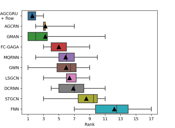
Figure 3: Boxplot of ranks of the top 10 algorithms across the four traffic datasets. The means of the ranks are shown by the black triangles; whiskers extend to the minimum and maximum ranks.

Table 1: Average MAE for PeMSD3, PeMSD4, PeMSD7, and PeMSD8 for 15/30/45/60 minutes horizons. The best and the second best results in each column are shown in bold and marked with underline respectively. Lower numbers are better.

Algorithm	MAE (15/ 30/ 45/ 60 min)
	PeMSD3	PeMSD4	PeMSD7	PeMSD8
DCRNN	14.42/15.87/17.10/18.29	1.38/1.78/2.06/2.29	2.23/3.06/3.67/4.18	1.16/1.49/1.70/1.87
STGCN	15.22/17.54/19.74/21.59	1.42/1.85/2.14/2.39	2.21/2.96/3.47/3.90	1.22/1.56/1.79/1.98
GWN	14.63/16.56/18.34/20.08	1.37/1.76/2.03/2.24	2.23/3.03/3.56/3.98	1.11/1.40/1.59/1.73
GMAN	14.73/15.44/16.15/16.96	1.38/1.61/1.76/1.88	2.40/2.76/2.98/3.16	1.23/1.36/1.46/1.55
AGCRN	14.20/15.34/16.28/17.38	1.41/1.67/1.84/2.01	2.19/2.81/3.15/3.42	1.16/1.39/1.53/1.67
LSGCN	14.28/16.08/17.77/19.23	1.40/1.78/2.03/2.20	2.23/2.99/3.50/3.95	1.21/1.54/1.75/1.89
FC-GAGA	14.68/15.85/16.40/17.04	1.43/1.78/1.95/2.06	2.22/2.85/3.18/3.36	1.18/1.47/1.62/1.72
DeepAR	15.84/18.15/20.30/22.64	1.51/2.01/2.38/2.68	2.53/3.61/4.48/5.20	1.25/1.61/1.87/2.10
DeepFactors	17.53/20.17/22.78/24.87	1.54/2.01/2.34/2.61	2.51/3.47/4.17/4.71	1.26/1.63/1.88/2.07
MQRNN	14.60/16.55/18.34/20.12	1.37/1.76/2.03/2.25	2.22/3.03/3.58/4.00	1.13/1.43/1.62/1.77
AGCGRU+flow	13.79/14.84/15.58/16.06	1.35/1.63/1.78/1.88	2.15/2.70/2.99/3.19	1.13/1.37/1.49/1.57

Table 2: Average MAE for PeMSD3, PeMSD4, PeMSD7, and PeMSD8 for 15/30/45/60 minutes horizons for the proposed flow based approach and deterministic encoder-decoder models. Lower numbers are better.

Algorithm	MAE (15/ 30/ 45/ 60 min)
	PeMSD3	PeMSD4	PeMSD7	PeMSD8
AGCGRU+flow	13.79/14.84/15.58/16.06	1.35/1.63/1.78/1.88	2.15/2.70/2.99/3.19	1.13/1.37/1.49/1.57
FC-AGCGRU	13.96/15.37/16.52/17.45	1.37/1.74/2.00/2.20	2.21/2.99/3.56/4.05	1.16/1.48/1.70/1.87
DCGRU+flow	14.48/15.67/16.52/17.36	1.38/1.71/1.92/2.08	2.19/2.87/3.29/3.61	1.17/1.44/1.58/1.70
FC-DCGRU	14.42/15.87/17.10/18.29	1.38/1.78/2.06/2.29	2.23/3.06/3.67/4.18	1.16/1.49/1.70/1.87
GRU+flow	14.40/16.10/17.63/19.18	1.37/1.76/2.02/2.23	2.24/3.02/3.55/3.96	1.12/1.41/1.59/1.74
FC-GRU	15.82/18.37/20.61/22.93	1.46/1.91/2.25/2.54	2.41/3.40/4.17/4.84	1.20/1.56/1.81/2.02

Figure 4: 15 minutes ahead predictions from the probabilistic forecasting algorithms with confidence intervals at node 4 of PeMSD7 dataset for the first day in the test set. The proposed AGCGRU+flow algorithm provides tighter confidence interval than its competitors, which leads to lower quantile error.

6 Experiments

We perform experiments on four graph-based and four non-graph based public datasets to evaluate proposed methods.

6.1 Datasets

We evaluate our proposed algorithm on four publicly available traffic datasets, namely PeMSD3, PeMSD4, PeMSD7 and PeMSD8. These are obtained from the Caltrans Performance Measurement System (PeMS) (Chen et al., 2000) and have been used in multiple previous works (Yu et al., 2018; Guo et al., 2019; Song et al., 2020; Bai et al., 2020; Huang et al., 2020). Each of these datasets consists of the traffic speed records, collected from loop detectors, and aggregated over 5 minute intervals, resulting in 288 data points per detector per day. In non-graph setting, we use Electricity (Dua & Graff, 2017) (hourly time-series of the electricity consumption), Traffic (Dua & Graff, 2017) (hourly occupancy rate, of different car lanes in San Francisco), Taxi (Salinas et al., 2019), and Wikipedia (Salinas et al., 2019) (count of clicks to different web links) datasets. The detailed statistics of these datasets are summarized in the supplementary material.

6.2 Preprocessing

For the PeMS datasets, missing values are filled by the last known value in the same series. The training, validation and test split is set at 70/10/20% chronologically and standard normalization of the data is used as in (Li et al., 2018). We use one hour of historical data ($P=12$) to predict the traffic for the next hour ($Q=12$). Graphs associated with the datasets are constructed using the procedure in (Huang et al., 2020).

6.3 Baselines

To demonstrate the effectiveness of our model, we compare to the following forecasting methods. A detailed description of each baseline is provided in the supplementary material.

Spatio-temporal point forecast models: DCRNN (Li et al., 2018), STGCN (Yu et al., 2018), ASTGCN (Guo et al., 2019), GWN (Wu et al., 2019), GMAN (Zheng et al., 2020), AGCRN (Bai et al., 2020), LSGCN (Huang et al., 2020).
Deep-learning based point forecasting methods:
DeepGLO (Sen et al., 2019), N-BEATS (Oreshkin et al., 2020), and FC-GAGA (Oreshkin et al., 2021).
Deep-learning based probabilistic forecasting methods: DeepAR (Salinas et al., 2020), DeepFactors (Wang et al., 2019), and MQRNN (Wen et al., 2017).

The detailed comparison of our approach with all of these models is provided in the supplementary material for space constraints. Here, we show results of a subset, focusing on those with the most competitive performance (Figure 3).

Table 3: Average CRPS, P10QL, P50QL, and P90QL for PeMSD3, PeMSD4, PeMSD7, and PeMSD8 for 15/30/45/60 minutes horizons. The best and the second best results in each column are shown in bold and marked with underline respectively. Lower numbers are better.

Dataset	PeMSD3	PeMSD4	PeMSD7	PeMSD8
Algorithm	CRPS (15/ 30/ 45/ 60 min)
DeepAR	11.41/13.11/14.62/16.27	1.13/1.52/1.82/2.07	1.92/2.78/3.44/3.99	0.94/1.24/1.46/1.64
DeepFactors	14.16/15.87/17.59/18.99	1.52/1.84/2.07/2.26	2.35/3.00/3.48/3.87	1.26/1.51/1.69/1.83
GRU+flow	11.23/12.70/13.98/15.25	1.14/1.50/1.75/1.95	1.88/2.61/3.09/3.46	0.95/1.23/1.42/1.57
DCGRU+flow	11.21/12.14/12.87/13.64	1.13/1.43/1.63/1.79	1.85/2.51/2.95/3.27	0.94/1.18/1.35/1.47
AGCGRU+flow	10.53/11.39/12.03/12.47	1.08/1.32/1.46/1.56	1.73/2.18/2.43/2.58	0.90/1.10/1.20/1.28
Algorithm	P10QL(%) (15/ 30/ 45/ 60 min)
DeepAR	4.11/4.69/5.21/5.69	1.37/1.96/2.45/2.86	2.56/3.90/4.92/5.78	1.14/1.59/1.93/2.24
DeepFactors	5.85/6.33/6.91/7.51	2.13/2.61/3.01/3.34	3.49/4.53/5.46/6.26	1.77/2.17/2.49/2.76
MQRNN	4.03/4.60/5.13/5.68	0.95/1.18/1.31/1.40	1.70/2.20/2.47/2.66	0.77/0.94/1.04/1.10
GRU+flow	4.19/4.71/5.14/5.55	1.36/1.87/2.25/2.56	2.50/3.57/4.29/4.85	1.12/1.52/1.80/2.04
DCGRU+flow	4.28/4.69/4.99/5.28	1.33/1.75/2.06/2.30	2.41/3.35/3.97/4.43	1.10/1.43/1.67/1.87
AGCGRU+flow	4.01/4.44/4.76/4.97	1.28/1.62/1.82/1.97	2.27/2.97/3.36/3.60	1.10/1.43/1.61/1.73
Algorithm	P50QL(%) (15/ 30/ 45/ 60 min)
DeepAR	9.11/10.44/11.68/13.03	2.37/3.15/3.73/4.20	4.35/6.21/7.70/8.95	1.97/2.52/2.94/3.30
DeepFactors	10.08/11.60/13.11/14.31	2.42/3.15/3.68/4.10	4.31/5.97/7.16/8.10	1.97/2.55/2.95/3.25
MQRNN	8.40/9.52/10.55/11.58	2.15/2.77/3.19/3.53	3.82/5.21/6.16/6.88	1.77/2.24/2.54/2.77
GRU+flow	8.28/9.26/10.15/11.04	2.16/2.76/3.17/3.50	3.84/5.19/6.10/6.81	1.76/2.21/2.49/2.72
DCGRU+flow	8.33/9.01/9.50/9.99	2.16/2.69/3.01/3.26	3.77/4.94/5.66/6.20	1.83/2.25/2.49/2.66
AGCGRU+flow	7.93/8.54/8.96/9.24	2.11/2.55/2.79/2.94	3.70/4.65/5.14/5.49	1.78/2.15/2.34/2.46
Algorithm	P90QL(%) (15/ 30/ 45/ 60 min)
DeepAR	4.40/5.13/5.70/6.40	1.10/1.45/1.67/1.84	2.13/3.03/3.65/4.08	0.93/1.22/1.40/1.53
DeepFactors	6.19/6.95/7.61/8.04	1.98/2.24/2.39/2.50	3.22/3.70/3.97/4.14	1.62/1.82/1.93/1.99
MQRNN	3.75/4.27/4.70/5.09	1.22/1.68/2.03/2.32	2.19/3.12/3.78/4.30	0.99/1.34/1.59/1.80
GRU+flow	4.33/4.94/5.48/6.04	1.11/1.43/1.63/1.77	2.02/2.74/3.16/3.44	0.93/1.18/1.33/1.44
DCGRU+flow	4.30/4.67/4.97/5.31	1.10/1.34/1.50/1.61	2.00/2.62/3.01/3.28	0.93/1.13/1.25/1.34
AGCGRU+flow	4.06/4.38/4.63/4.82	1.05/1.26/1.37/1.45	1.83/2.25/2.48/2.62	0.87/1.01/1.09/1.14

6.4 Hyperparameters and training setup

For our model, we use an $L=2$ layer AGCGRU (Bai et al., 2020) as the state-transition function. The dimension of the learnable node embedding is $d_{e}=10$, and the number of RNN units is $d_{x}=64$. We treat $\rho$ and $\sigma$ as fixed hyperparameters and set $\rho=1$ and $\sigma=0$ (no process noise). We train for 100 epochs using the Adam optimizer, with a batch size of 64. The initial learning rate is set to 0.01 and we follow a decaying schedule as in (Li et al., 2018). Hyperparameters associated with scheduled sampling (Bengio et al., 2015), gradient clipping, and early stoppng are borrowed from (Li et al., 2018). We set the number of particles $N_{p}=1$ during training and $N_{p}=10$ for validation and testing. The number of exponentially spaced discrete steps (Li & Coates, 2017) for integrating the flow is $N_{\lambda}=29$. For each dataset, we conduct two separate experiments minimizing the training MAE (results are used to report MAE, MAPE, RMSE, and P50QL) and the training negative log posterior probability (results are used to report CRPS, P10QL, and P90QL). We also experiment with alternative state transition functions, including the DCGRU (Li et al., 2018) and GRU (Chung et al., 2014). For these, the hyperparameters are fixed to the same values as presented above.

6.5 Results and Discussion

Comparison with baselines :

Results for the point forecasting task are summarized in Table 1. We observe that most of the spatio-temporal models perform better than graph agnostic baselines in most cases. Moreover, the proposed AGCGRU+flow algorithm achieves on par or better performance with the best-performing spatio-temporal models, such as GWN, GMAN and AGCRN. We present a comparison of the average rankings across datasets in Figure 3. Our proposed method achieves the best average ranking and significantly outperforms the baseline methods. Table 3 summarizes the results for probabilistic forecasting. We observe that in most cases, the proposed flow based algorithms outperform the competitors. MQRNN also shows impressive performance in predicting the forecast quantiles, as it is explicitly trained to minimise the quantile losses. In particular, comparison of GRU+flow with the DeepAR model reveals that even without a sophisticated RNN architecture, the particle flow based approach shows better characterization of prediction uncertainty in most cases. Figure 4 provides a qualitative comparison of the uncertainty characterization, showing example confidence intervals for 15-minute ahead prediction for the PeMSD7 dataset. We see that the proposed algorithm provides considerably tighter intervals, while still achieving coverage of the observed values.

Generalization of particle flow inference across architectures :

Table 2 shows that in comparison to deterministic encoder-decoder based sequence to sequence prediction models, the proposed flow based approaches perform better in almost all cases for three different architectures of the RNN. In each case, both of the encoder-decoder model and our approach use a 2-layer architecture with 64 RNN units.

Comparison to the particle filter :

Table 4 demonstrates the effectiveness of particle flow (Daum & Huang, 2007), comparing it to a Bootstrap Particle Filter (BPF) (Gordon et al., 1993) with the same number of particles. The use of the bootstrap particle filter leads to a computationally faster algorithm (requiring approximately 60% of the training time of the particle flow-based method).

Table 4: Average MAE and average CRPS for PeMSD3, PeMSD4, PeMSD7, and PeMSD8 for 15/30/45/60 minutes horizons for AGCGRU+flow and AGCGRU+BPF. Lower numbers are better.

Dataset	PeMSD3	PeMSD4	PeMSD7	PeMSD8
Algorithm	MAE (15/ 30/ 45/ 60 min)
AGCGRU+flow	13.79/14.84/15.58/16.06	1.35/1.63/1.78/1.88	2.15/2.70/2.99/3.19	1.13/1.37/1.49/1.57
AGCGRU+BPF	14.19/15.13/15.85/16.35	1.36/1.65/1.80/1.90	2.19/2.73/2.99/3.17	1.18/1.41/1.52/1.59
Algorithm	CRPS (15/ 30/ 45/ 60 min)
AGCGRU+flow	10.53/11.39/12.03/12.47	1.08/1.32/1.46/1.56	1.73/2.18/2.43/2.58	0.90/1.10/1.20/1.28
AGCGRU+BPF	11.32/11.94/12.55/12.92	1.10/1.32/1.45/1.54	1.79/2.24/2.49/2.66	0.96/1.13/1.22/1.28

Table 5: Average CRPS for PeMSD3, PeMSD4, PeMSD7, and PeMSD8 for 15/30/45/60 minutes horizons for AGCRN-ensemble, GMAN-ensemble, and AGCGRU+flow. The best result in each column is shown in bold. Lower numbers are better.

Algorithm	CRPS (15/ 30/ 45/ 60 min)
	PeMSD3	PeMSD4	PeMSD7	PeMSD8
AGCRN-ensemble	12.64/13.44/13.96/14.27	1.20/1.44/1.56/1.68	1.90/2.39/2.60/2.81	1.03/1.20/1.28/1.38
GMAN-ensemble	12.79/13.49/14.13/14.77	1.16/1.38/1.51/1.62	1.96/2.31/2.53/2.73	0.95/1.10/1.19/1.28
AGCGRU+flow	10.53/11.39/12.03/12.47	1.08/1.32/1.46/1.56	1.73/2.18/2.43/2.58	0.90/1.10/1.20/1.28

Table 6: Normalized Deviation on Electricity and Traffic datasets. The best and the second best results in each column are shown in bold and marked with underline respectively. Lower numbers are better.

Algorithm	Electricity				Traffic
	2014-09-01	2014-03-31	2014-12-18	last 7 days	2008-06-15	2008-01-14	last 7 days
TRMF	0.160	n/a	0.104	0.255	0.200	n/a	0.187
DeepAR	0.070	0.272	0.086	n/a	0.170	0.296	0.140
DeepState	0.083	n/a	n/a	n/a	0.167	n/a	n/a
DeepFactors	n/a	0.112	n/a	n/a	n/a	0.225	n/a
DeepGLO	n/a	n/a	0.082	n/a	n/a	n/a	0.148
N-BEATS	0.064	0.065	n/a	0.171	0.114	0.230	0.110
FC-GRU	0.102	0.118	0.098	0.203	0.259	0.528	0.233
GRU+flow	0.070	0.071	0.069	0.140	0.133	0.322	0.125

Table 7: Average $\text{CRPS}_{sum}$ for Electricity, Traffic, Taxi, and Wikipedia datasets. The best and the second best results in each column are shown in bold and marked with underline respectively. Lower numbers are better

Dataset	Vec-LSTM ind-scaling	Vec-LSTM lowrank-Copula	GP scaling	GP Copula	LSTM Real-NVP	LSTM MAF	Transformer MAE	GRU+ flow
Electricity	0.025	0.064	0.022	0.024	0.024	0.021	0.021	0.013
Traffic	0.087	0.103	0.079	0.078	0.078	0.069	0.056	0.028
Taxi	0.506	0.326	0.183	0.208	0.175	0.161	0.179	0.140
Wikipedia	0.133	0.241	1.483	0.086	0.078	0.067	0.063	0.054

Comparison to ensembles :

We compare the proposed approach with an ensemble of competitive deterministic forecasting techniques. We choose the size of the ensemble so that the algorithms have an approximately equal execution time. We use AGCRN and GMAN to form the ensembles, as they are the best point-forecast baseline algorithms. From Table 5, we observe that the proposed AGCGRU+flow achieves lower average CRPS compared to the ensembles in all cases.

Point forecasting results on non-graph datasets :

We evaluate our proposed flow-based RNN on the Electricity and Traffic datasets, following the setting described in Appendix C.4 in (Oreshkin et al., 2020). We augment the results table in (Oreshkin et al., 2020) with the results from an FC-GRU (a fully connected GRU encoder-decoder) and GRU+flow. We use a 2 layer GRU with 64 RNN units in both cases. We follow the preprocessing steps in (Oreshkin et al., 2020). In the literature, four different data splits have been used for the Electricity dataset, and three different splits have been used for the Traffic dataset. The evaluation metric is P50QL (Normalized Deviation).

In Table 6, we observe that the flow based approach performs comparably or better than the state-of-the-art N-BEATS algorithm for the Electricity dataset, even with a simple GRU as the state transition function. The better performance of the univariate N-BEATS compared to the multivariate models suggests that most time-series in these datasets do not provide valuable additional information for predicting other datasets. This is in contrast to the graph-based datasets, where the performance of N-BEATS was considerably worse than the multivariate algorithms. The proposed flow-based algorithm achieves prediction performance on the Traffic dataset that is comparable to N-BEATS except for one split with limited training data. Across all datasets and split settings, our flow-based approach significantly outperforms the FC-GRU. The proposed algorithm outperforms TRMF, DeepAR, DeepState and DeepGLO. It outperforms DeepFactors for the Electricity dataset, but is worse for the Traffic dataset (for the same split with limited available training data).

Probabilistic forecasting results on non-graph datasets :

For comparison with state-of-the-art deep learning based probabilistic forecasting methods on standard non-graph time-series datasets, we evaluate the proposed GRU+flow algorithm following the setting in (Rasul et al., 2021). The results reported in Table 1 of (Rasul et al., 2021) are augmented with the results of the GRU+flow algorithm. We use a 2 layer GRU with 64 RNN units in each case. We follow the preprocessing steps as in (Salinas et al., 2019; Rasul et al., 2021). The evaluation metric is (normalized) $\text{CRPS}_{sum}$ (defined in the supplementary material), which is obtained by first summing across the different time-series, both for the ground-truth test data, and samples of forecasts, and then computing the (normalized) CRPS on the summed data. The results are summarized in Table 7. We observe that the proposed GRU+flow achieves the lowest $\text{CRPS}_{sum}$ for all datasets.

Computational complexity :

For simplicity, we consider a GRU instead of a graph convolution based RNN and we only focus on one sequence instead of a batch. Our model has to perform both GRU computation and particle flow for the first $P$ time steps and then apply the GRU and the linear projection for the next $Q$ steps to generate the predictions. For an $L$-layer GRU with $d_{x}$ RNN units and $N$-dimensional input, the complexity of the GRU operation for $N_{p}$ particles is $\mathcal{O}((P+Q)N_{p}LNd_{x}^{2})$ (Chung et al., 2014). The total complexity of the EDH particle flow (Choi et al., 2011) is $\mathcal{O}(PN_{\lambda}N^{3})$ for computing the flow parameters and $\mathcal{O}(PN_{p}N_{\lambda}Nd_{x}^{2})$ for applying the particle flow (more details in the supplementary material). The total complexity of the measurement model for $N_{p}$ particles is $\mathcal{O}(QN_{p}Nd_{x}^{2})$. Since in most cases $N\gg d_{x}$ and $N\gg N_{p}$, the complexity of our algorithm for forecasting of one sequence is $\mathcal{O}(PN_{\lambda}N^{3})$. Many of the other algorithms exhibit a similar $\mathcal{O}(N^{3})$ complexity, e.g. TRMF, GMAN. We specify the execution time and memory usage in the supplementary material. Scaling the proposed methodology to extremely high dimensional settings is of significant importance and can be addressed in several ways. For spatio-temporal predictions using the graph-based recurrent architectures, this can be done if the graph can be partitioned meaningfully. For non-graph datasets, we can use the cross-correlation among different time-series to group them into several lower-dimensional problems. Alternatively, we can train a univariate model based on all the time-series as in (Rangapuram et al., 2018).

7 Conclusion

In this paper, we propose a state-space probabilistic modeling framework for multivariate time-series prediction that can process information provided in the form of a graph that specifies (probable) predictive or causal relationships. We develop a probabilistic forecasting algorithm based on the Bayesian inference of hidden states via particle flow. For spatio-temporal forecasting, we use GNN based architectures to instantiate the framework. Our method demonstrates comparable or better performance in point forecasting and considerably better performance in uncertainty characterization compared to existing techniques.

Supplementary Material

8 Particle flow for Bayesian inference in a state-space model

8.1 Background

Particle flow is an alternative to particle filters for Bayesian filtering in a state-space model. Recall the first order Markov model specified in eqs. (4), (5), and (6) in Section 5.1 of the main paper.

$$\mathbf{x}_{1} \sim p_{1}(\cdot,\mathbf{z}_{1},\rho)\,,$$ (15)

$$\mathbf{x}_{t} =g_{\mathcal{G},\psi}(\mathbf{x}_{t-1},\mathbf{y}_{t-1},\mathbf{z}_{t},\mathbf{v}_{t}),\text{ for }t>1\,,$$ (16)

$$\mathbf{y}_{t} =h_{\mathcal{G},\phi}(\mathbf{x}_{t},\mathbf{z}_{t},\mathbf{w}_{t}),\text{ for }t\geqslant 1\,.$$ (17)

Here $\mathbf{y}_{t}$ is the observation from the state-space model at time $t$. $\mathbf{x}_{t}$ and $\mathbf{z}_{t}$ denote the unobserved state variable and observed covariates at time $t$ respectively. The filtering task is to compute the posterior distribution of the state trajectory $p_{\Theta}(\mathbf{x}_{t}|\mathbf{y}_{1:t},\mathbf{z}_{1:t})$ recursively. Suppose we have a set of $N_{p}$ samples (particles) $\{\mathbf{x}_{t-1}\}_{j=1}^{N_{p}}$ which approximates the posterior distribution of $\mathbf{x}_{t-1}$.

$$p_{\Theta}(\mathbf{x}_{t-1}|\mathbf{y}_{1:t-1},\mathbf{z}_{1:t-1})\approx\frac{1}{N_{p}}\sum_{j=1}^{N_{p}}\delta(\mathbf{x}_{t-1}-\mathbf{x}_{t-1}^{j})\,.$$ (18)

In the ‘predict’ step, we approximate the predictive posterior distribution at time $t$ as follows:

$$p_{\Theta}(\mathbf{x}_{t}|\mathbf{y}_{1:t-1},\mathbf{z}_{1:t}) =\int p_{\psi,\sigma}(\mathbf{x}_{t}|\mathbf{x}_{t-1},\mathbf{y}_{t-1},\mathbf{z}_{t})\,$$

$$\qquad p_{\Theta}(\mathbf{x}_{t-1}|\mathbf{y}_{1:t-1},\mathbf{z}_{1:t-1})d\mathbf{x}_{t-1}\,,$$

$$\approx\frac{1}{N_{p}}\sum_{j=1}^{N_{p}}\delta(\mathbf{x}_{t}-\mathbf{\tilde{x}}_{t}^{j})\,,$$ (19)

where, the particles $\{\mathbf{\tilde{x}}_{t}^{j}\}_{j=1}^{N_{p}}$ from the predictive posterior distribution $p_{\Theta}(\mathbf{x}_{t}|\mathbf{y}_{1:t-1},\mathbf{z}_{1:t})$ are obtained by propagating $\{\mathbf{x}_{t-1}^{j}\}_{j=1}^{N_{p}}$ through the state-transition model specified by eq. (16). Subsequently, the ‘update’ step applies Bayes’ theorem to compute the posterior distribution at time $t$ as follows:

$$p_{\Theta}(\mathbf{x}_{t}|\mathbf{y}_{1:t},\mathbf{z}_{1:t})\propto p_{\Theta}(\mathbf{x}_{t}|\mathbf{y}_{1:t-1},\mathbf{z}_{1:t})p_{\phi,\gamma}(\mathbf{y}_{t}|\mathbf{x}_{t},\mathbf{z}_{t})\,.$$ (20)

For non-linear state space models, particle filters (Gordon et al., 1993; Doucet & Johansen, 2009) employ importance sampling to approximate the ‘update’ step in eq. (20). However, constructing well-matched proposal distributions to the posterior distribution in high-dimensional state-spaces is extremely challenging. A mismatch between the proposal and the posterior leads to weight degeneracy after resampling, which results in poor performance of particle filters in high-dimensional problems (Bengtsson et al., 2008; Snyder et al., 2008; Beskos et al., 2014). Instead of sampling, particle flow filters offer a significantly better solution in complex problems by transporting particles continuously from the prior to the posterior (Daum & Huang, 2007; Ding & Coates, 2012; Daum & Huang, 2014; Daum et al., 2017).

8.2 Particle flow

Figure 5: Migration of particles from a 2-d Gaussian prior to a 2-d Gaussian posterior distribution. a) The samples (asterisk) from the prior distribution, b) The contours of the posterior distribution and the direction of flow for the particles at an intermediate step, c) The particles after the flow, approximately distributed according to the posterior distribution.

In a given time step $t$, particle flow algorithms (Daum & Huang, 2007; Daum et al., 2010) solve differential equations to gradually migrate particles from the predictive distribution such that they represent the posterior distribution for the same time step after the flow. A particle flow can be modelled by a background stochastic process $\eta_{\lambda}$ in a pseudo-time interval $\lambda\in[0,1]$, such that the distribution of $\eta_{0}$ is the predictive distribution $p_{\Theta}(\mathbf{x}_{t}|\mathbf{y}_{1:t-1},\mathbf{z}_{1:t})$ and the distribution of $\eta_{1}$ is the posterior distribution $p_{\Theta}(\mathbf{x}_{t}|\mathbf{y}_{1:t},\mathbf{z}_{1:t})$. Since particle flow only considers migration of particles within a single time step, we omit the time index $t$ in $\eta_{\lambda}$, $\mathbf{y}$, and $\mathbf{z}$ to simplify notation.

In (Daum et al., 2010), an ordinary differential equation (ODE) with zero diffusion governs the flow of $\eta_{\lambda}$:

$$\dfrac{d\eta_{\lambda}}{d\lambda}=\varphi(\eta_{\lambda},\lambda)\,\,.$$ (21)

If the predictive distribution and the additive measurement noise is Gaussian and the measurement function $h$ is linear, the Exact Daum-Huang (EDH) flow is given as:

$$\varphi(\eta_{\lambda},\lambda)=A(\lambda)\eta_{\lambda}+b(\lambda)\,\,,$$ (22)

where,

$$A(\lambda) =-\dfrac{1}{2}\bar{P}H^{T}(\lambda H\bar{P}H^{T}+R)^{-1}H\,\,,$$ (23)

$$b(\lambda) =(I+2\lambda A(\lambda))[(I+\lambda A(\lambda))\bar{P}H^{T}R^{-1}\mathbf{y}+A(\lambda)\bar{\eta}_{0}]\,\,,$$ (24)

Here $\bar{\eta}_{0}$ and $\bar{P}$ are the mean vector and the covariance matrix of the predictive distribution respectively. For a general nonlinear state-space model, we usually a Gaussian approximation of the predictive distribution based on sample estimates of $\bar{\eta}_{0}$ and $\bar{P}$ or via the Extended Kalman Filter (EKF). $\mathbf{y}$ denotes the new observation at time $t$. The linear measurement model in $\mathbf{x}$ is specified by the measurement matrix $H=\frac{h_{\mathcal{G},\phi}(\mathbf{x},\mathbf{z},\mathbf{0})}{\partial\mathbf{x}}$, and $R$ denotes the covariance matrix of the zero mean additive Gaussian measurement noise. For a nonlinear measurement model, we use a first order Taylor series approximation at the mean of the particles $\bar{\eta}_{\lambda}$ and replace $H$ by $H(\lambda)=\frac{\partial h_{\mathcal{G},\phi}(\eta,\mathbf{z},\mathbf{0})}{\partial\eta}\Bigg{|}_{\eta=\bar{\eta}_{\lambda}}$ and $\mathbf{y}$ by $\big{(}\mathbf{y}-e(\lambda)\big{)}$, where the linearization error $e(\lambda)=h_{\mathcal{G},\phi}(\bar{\eta}_{\lambda},\mathbf{z},\mathbf{0})-H(\lambda)\bar{\eta}_{\lambda}$ in eq. (23) and (24). Similarly, for a zero mean non-Gaussian measurement noise, we use a Gaussian approximation to replace $R$ in eq. (23) and (24) by $R(\lambda)=\mathrm{Cov}\left[\mathbf{y}|\bar{\eta}_{\lambda},\mathbf{z}\right]$. A detailed description of the implementation of the exact Daum-Huang (EDH) filter is provided in (Choi et al., 2011).

Algorithm 2 Particle flow

1:  Input: $\{\eta_{0}^{j}=\mathbf{\tilde{x}}_{t}^{j}\}_{j=1}^{N_{p}}$, $\mathbf{y}_{t}$, $\mathbf{z}_{t}$, $\{\epsilon_{m}\}_{m=1}^{N_{\lambda}}$, and $\Theta$

2:  Output: $\{\mathbf{x}_{t}^{j}=\eta_{1}^{j}\}_{j=1}^{N_{p}}$

3:  Compute $\bar{\eta}_{0}=\frac{1}{N_{p}}\sum_{j=1}^{N_{p}}\eta_{0}^{j}$

4:  Compute $\bar{P}=\frac{1}{N_{p}}\sum_{j=1}^{N_{p}}\left[(\eta_{0}^{j}-\bar{\eta}_{0})(\eta_{0}^{j}-\bar{\eta}_{0})^{T}\right]$

5:  Set $\lambda_{0}=0$

6:  for $m=1,2,...,N_{\lambda}$ do

7:     $\lambda_{m}=\lambda_{m-1}+\epsilon_{m}$

8:     Linearize the measurement model at $\bar{\eta}_{\lambda_{m-1}}=\frac{1}{N_{p}}\sum_{j=1}^{N_{p}}\eta_{\lambda_{m-1}}^{j}$ to compute $H(\lambda_{m-1})$ and $e(\lambda_{m-1})$.

9:     Compute $R(\lambda_{m-1})=\textbf{Cov}\left[\mathbf{y}_{t}|\bar{\eta}_{\lambda_{m-1}},\mathbf{z}_{t}\right]$.

10:     Compute $A(\lambda_{m-1})$ and $b(\lambda_{m-1})$ using eq. (23) and (24).

11:     Apply particle flow to all particles: $\eta_{m}^{j}=\eta_{m-1}^{j}+\epsilon_{m}\big{(}A(\lambda_{m-1})\eta_{m-1}^{j}+b(\lambda_{m-1})\big{)}$

12:  end for

13:  Set $\mathbf{x}_{t}^{j}=\eta_{1}^{j}$ for $1\leqslant j\leqslant N_{p}$

Numerical integration is usually used to solve the ODE in Equation (22). The integral between $\lambda_{m-1}$ and $\lambda_{m}$ for $1\leqslant m\leqslant N_{\lambda}$, where $\lambda_{0}=0$ and $\lambda_{N_{\lambda}}=1$, is approximated via the Euler update rule. For the $j$-th particle, the EDH flow in the $m$-th pseudo-time interval becomes:

$$\eta_{\lambda_{m}}^{j} =\eta_{\lambda_{m-1}}^{j}+\epsilon_{m}\big{(}A(\lambda_{m-1})\eta_{\lambda_{m-1}}^{j}+b(\lambda_{m-1})\big{)}\,,$$ (25)

where the step size $\epsilon_{m}=\lambda_{m}-\lambda_{m-1}$ and $\displaystyle\sum_{m=1}^{N_{\lambda}}\epsilon_{m}=1$. We start the particle flow from $\eta_{0}^{j}=\mathbf{\tilde{x}}_{t}^{j}$ and after the flow is complete, we set $\mathbf{x}_{t}^{j}=\eta_{1}^{j}$ to approximate the posterior distribution of $\mathbf{x}_{t}$ as:

$$p_{\Theta}(\mathbf{x}_{t}|\mathbf{y}_{1:t},\mathbf{z}_{1:t})\approx\frac{1}{N_{p}}\sum_{j=1}^{N_{p}}\delta(\mathbf{x}_{t}-\mathbf{x}_{t}^{j})\,.$$ (26)

The overall EDH particle flow algorithm is summarized in Algorithm 2. Figure 5 demonstrates the migration of the particles from the prior to the posterior distribution for a Gaussian predictive distribution and a linear-Gaussian measurement model.

9 Model training

Algorithm 3 summarizes the learning of the model parameters $\Theta$, described in Section 5.2.2 of the main paper.

Algorithm 3 Model training and testing

1:  Input: Training and test data: $\{\mathbf{y}_{1:P+Q}^{(m)},$ $\mathbf{z}_{1:P+Q}^{(m)}\}_{m\in\mathcal{D}_{trn}}$, $\{\mathbf{y}_{1:P}^{(n)},\mathbf{z}_{1:P+Q}^{(n)}\}_{n\in\mathcal{D}_{test}}$

2:  Output: $\{\hat{p}_{\hat{\Theta}}(\mathbf{y}_{P+1:P+Q}^{(n)}|\mathbf{y}_{1:P}^{(n)},\mathbf{z}_{1:P+Q}^{(n)})\}_{n\in\mathcal{D}_{test}}$

3:  Hyperparameters: Number of iterations $N_{iter}$, step-size $\{\zeta_{k}\}_{k=1}^{N_{iter}}$

4:  Initialization: random initialization for the system parameters $\Theta_{0}$

5:  Model training:

6:  Set $k=1$

7:  while $k\leqslant N_{iter}$ do

8:     Sample a minibatch $\mathcal{D}\subset\mathcal{D}_{trn}$.

9:     Compute the approximate posterior distribution of the forecasts $\{\hat{p}_{\Theta_{k-1}}(\mathbf{y}_{P+1:P+Q}^{(m)}|\mathbf{y}_{1:P}^{(m)},\mathbf{z}_{1:P+Q}^{(m)})\}_{m\in\mathcal{D}}$ using Algorithm 1 in the main paper with the current parameters $\Theta_{k-1}$.

10:     Compute the gradient of the chosen loss function $\mathcal{L}(\Theta,\mathcal{D})$ w.r.t. model parameters $\Theta$ at $\Theta_{k-1}$

11:     Update the system parameters using SGD algorithm: $\Theta_{k}=\Theta_{k-1}-\zeta_{k}\nabla_{\Theta}\mathcal{L}(\Theta,\mathcal{D})\big{|}_{\Theta=\Theta_{k-1}}$

12:     $k=k+1$

13:  end while

14:  Save the estimated model $\widehat{\Theta}=\Theta_{N_{iter}}$

15:  Testing:

16:  Compute the test set forecast posterior distributions $\{\hat{p}_{\hat{\Theta}}(\mathbf{y}_{P+1:P+Q}^{(n)}|\mathbf{y}_{1:P}^{(n)},\mathbf{z}_{1:P+Q}^{(n)})\}_{n\in\mathcal{D}_{test}}$ using Algorithm 1 in the main paper with the estimated model parameters $\widehat{\Theta}$.

10 Description and statistics of datasets

Table 8: Summary statistics of the PeMS road traffic datasets

Dataset	PeMSD3	PeMSD4	PeMSD7	PeMSD8
No. nodes	358	307	228	170
No. time steps	26208	16992	12672	17856
Interval	5 min	5 min	5 min	5 min

The statistics of the PeMS datasets and the non-graph datasets used in our experiments are summarized in Tables 8 and 9 respectively. The description of the PeMS datasets are provided in Section 6.1 of the main paper. The Electricity dataset contains electricity consumption for 370 clients. The Traffic dataset is composed of 963 time-series of lane occupancy rates. The Taxi dataset contains counts of taxis on different roads and the Wikipedia dataset specifies clicks to web links.

Table 9: Summary statistics of the multivariate non-graph datasets

Dataset	No. time series (N)	Domain	Freq.	No. time steps	Prediction length (Q)
Electricity	370	$\mathbb{R}^{+}$	Hourly	5833	24
Traffic	963	$(0,1)$	Hourly	4001	24
Taxi	1214	$\mathbb{N}$	30 Minutes	1488	24
Wikipedia	2000	$\mathbb{N}$	Daily	792	30

11 Definitions of evaluation metrics

The point forecasts are evaluated by computing mean absolute error (MAE), mean absolute percentage error (MAPE), and root mean squared error (RMSE). For the test-set indexed by $\mathcal{D}_{test}$, let $\mathbf{y}_{t}^{(m)}\in\mathbb{R}^{N}$ and $\mathbf{\hat{y}}_{t}^{(m)}\in\mathbb{R}^{N}$ denote the ground truth and the prediction at horizon $t$ for $m$-th test example respectively. The average MAE, MAPE, and RMSE at horizon $t$ are defined as follows:

$$\text{MAE}(\mathcal{D}_{test},t) =\frac{1}{N\lvert\mathcal{D}_{test}\rvert}\sum_{m\in\mathcal{D}_{test}}\lvert\lvert\mathbf{y}_{t}^{(m)}-\mathbf{\hat{y}}_{t}^{(m)}\rvert\rvert_{1}\,,$$ (27)

$$\text{MAPE}(\mathcal{D}_{test},t) =\frac{1}{N\lvert\mathcal{D}_{test}\rvert}\sum_{m\in\mathcal{D}_{test}}\sum_{i=1}^{N}\frac{\lvert\mathbf{y}_{t,i}^{(m)}-\mathbf{\hat{y}}_{t,i}^{(m)}\rvert}{\lvert\mathbf{y}_{t,i}^{(m)}\rvert}\,,$$ (28)

$$\text{RMSE}(\mathcal{D}_{test},t) =\sqrt{\frac{1}{N\lvert\mathcal{D}_{test}\rvert}\sum_{m\in\mathcal{D}_{test}}\lvert\lvert\mathbf{y}_{t}^{(m)}-\mathbf{\hat{y}}_{t}^{(m)}\rvert\rvert_{2}^{2}}\,,$$ (29)

For comparison among the probabilistic forecasting models, we compute the Continuous Ranked Probability Score (CRPS) (Gneiting & Raftery, 2007), and the P10 and P90 Quantile Losses (QL) (Salinas et al., 2020; Wang et al., 2019). Let $F(\cdot)$ be the Cumulative Distribution Function (CDF) of the forecast of the true value $x\in\mathbb{R}$. We denote by $\mathbf{1}\{x\leqslant z\}$ the indicator function that attains the value 1 if $x\leqslant z$ and the value 0 otherwise. The continuous ranked probability score (CRPS) is defined as:

$$\text{CRPS}(F,x)=\int_{-\infty}^{\infty}\Big{(}F(z)-\mathbf{1}\{x\leqslant z\}\Big{)}^{2}dz\,.$$ (30)

CRPS is a proper scoring function, i.e., it attains its minimum value of zero when the forecast CDF $F$ is a step function at the ground truth $x$. The average CRPS at horizon $t$ is defined as the average marginal CRPS across different time-series.

$$\text{CRPS}_{avg}(\mathcal{D}_{test},t)=\,$$

$$\qquad\frac{1}{N\lvert\mathcal{D}_{test}\rvert}\sum_{m\in\mathcal{D}_{test}}\sum_{i=1}^{N}\text{CRPS}(F_{t,i}^{(m)},\mathbf{y}_{t,i}^{(m)})\,,$$ (31)

where $F_{t,i}^{(m)}(\cdot)$ is the marginal CDF of the forecast at horizon $t$ for $i$-th time-series in $m$-th test example.

Let $F_{t,sum}^{(m)}(\cdot)$ is the CDF of the sum of the forecasts of all time-series at horizon $t$ in $m$-th test example. The (normalized) $\text{CRPS}_{sum}$ is defined as:

$$\text{CRPS}_{sum}(\mathcal{D}_{test})=\,$$

$$\qquad\frac{\sum_{t}\sum_{m\in\mathcal{D}_{test}}\text{CRPS}(F_{t,sum}^{(m)},\sum_{i=1}^{N}\mathbf{y}_{t,i}^{(m)})}{\sum_{t}\sum_{m\in\mathcal{D}_{test}}\lvert\sum_{i=1}^{N}\mathbf{y}_{t,i}^{(m)}\rvert}\,.$$ (32)

For a given quantile $\alpha\in(0,1)$, a true value $x$, and an $\alpha$-quantile prediction $\hat{x}(\alpha)=F^{-1}(\alpha)$, the $\alpha$-quantile loss is defined as:

$$\text{QL}\big{(}x,\hat{x}(\alpha)\big{)}=2\Bigg{(}\alpha\big{(}x-\hat{x}(\alpha)\big{)}\mathbf{1}\{x>\hat{x}(\alpha)\}+\,$$

$$\qquad\qquad(1-\alpha)\big{(}\hat{x}(\alpha)-x\big{)}\mathbf{1}\{x\leqslant\hat{x}(\alpha)\}\Bigg{)}\,.$$ (33)

The average (normalized) quantile loss (QL) is defined as follows:

$$\text{QL}_{avg}(\mathcal{D}_{test},t,\alpha)=\frac{\sum_{m\in\mathcal{D}_{test}}\sum_{i=1}^{N}\text{QL}\big{(}\mathbf{y}_{t,i}^{(m)},\mathbf{\hat{y}}_{t,i}^{(m)}(\alpha)\big{)}}{\sum_{m\in\mathcal{D}_{test}}\sum_{i=1}^{N}\lvert\mathbf{y}_{t,i}^{(m)}\rvert}\,.$$ (34)

The P10QL metric is obtained by setting $\alpha=0.1$ in eq. (34); the P90QL metric corresponds to $\alpha=0.9$ and the ND (P50QL) metric is obtained using $\alpha=0.5$.

Table 10: Average MAE, MAPE and RMSE for PeMSD3 dataset for 15/30/45/60 minutes horizons. The best and the second best results in each column are shown in bold and marked with underline respectively. Lower numbers are better.

Algorithm	PeMSD3 (15/ 30/ 45/ 60 min)
	MAE	MAPE(%)	RMSE
HA	31.58	33.78	52.39
ARIMA	17.31/22.12/27.35/32.47	16.53/20.78/25.66/30.84	26.80/34.60/42.37/49.98
VAR	18.59/20.80/23.06/24.86	19.59/21.81/24.24/26.44	31.05/33.92/36.93/39.32
SVR	16.66/20.33/24.33/28.34	16.07/19.45/23.31/27.57	25.97/32.19/38.30/44.57
FNN	16.87/20.30/23.91/27.74	19.59/23.67/30.09/35.44	25.46/30.97/36.27/41.86
FC-LSTM	19.01/19.46/19.92/20.29	19.77/20.23/20.82/21.30	32.96/33.59/34.24/34.83
DCRNN	14.42/15.87/17.10/18.29	14.57/15.78/16.87/17.95	24.33/27.05/28.99/30.76
STGCN	15.22/17.54/19.74/21.59	16.22/18.44/20.13/21.88	26.20/29.10/32.19/34.83
ASTGCN	17.03/18.50/19.58/20.95	18.02/19.28/20.18/21.61	29.04/31.81/33.98/36.37
GWN	14.63/16.56/18.34/20.08	13.74/15.24/16.82/18.75	25.06/28.48/31.11/33.58
GMAN	14.73/15.44/16.15/16.96	15.63/16.25/16.99/17.91	24.48/25.68/26.80/27.99
AGCRN	14.20/15.34/16.28/17.38	13.79/14.47/15.14/16.25	24.75/26.61/28.06/29.61
LSGCN	14.28/16.08/17.77/19.23	14.80/16.01/17.15/18.21	25.88/28.11/30.31/32.37
DeepGLO	14.79/18.89/19.11/23.53	14.12/16.92/17.75/21.68	22.97/29.17/30.48/35.64
N-BEATS	15.57/18.12/20.50/23.03	15.56/18.05/20.50/23.19	24.44/28.69/32.62/36.72
FC-GAGA	14.68/15.85/16.40/17.04	15.57/15.88/16.32/17.16	24.65/26.85/27.90/28.97
DeepAR	15.84/18.15/20.30/22.64	16.26/18.42/20.19/22.56	26.33/29.96/33.12/36.65
DeepFactors	17.53/20.17/22.78/24.87	19.22/24.42/29.58/34.43	27.62/31.83/35.36/37.91
MQRNN	14.60/16.55/18.34/20.12	15.17/17.34/18.94/20.66	25.35/28.77/31.50/34.40
AGCGRU+flow	13.79/14.84/15.58/16.06	14.01/14.75/15.34/15.80	22.08/24.26/25.55/26.43

Table 11: Average MAE, MAPE and RMSE for PeMSD4 dataset for 15/30/45/60 minutes horizons. The best and the second best results in each column are shown in bold and marked with underline respectively. Lower numbers are better.

Algorithm	PeMSD4 (15/ 30/ 45/ 60 min)
	MAE	MAPE(%)	RMSE
HA	3.16	7.00	6.13
ARIMA	1.53/2.01/2.37/2.68	2.92/4.06/4.96/5.73	3.11/4.36/5.25/5.95
VAR	1.66/2.12/2.39/2.57	3.27/4.33/4.95/5.36	3.09/4.02/4.51/4.83
SVR	1.48/1.91/2.23/2.49	2.88/3.97/4.86/5.61	3.11/4.29/5.08/5.66
FNN	1.48/1.90/2.23/2.51	3.04/4.09/4.98/5.80	3.08/4.27/5.08/5.68
FC-LSTM	2.20/2.22/2.23/2.26	4.95/4.97/4.99/5.05	4.89/4.92/4.95/5.01
DCRNN	1.38/1.78/2.06/2.29	2.69/3.72/4.51/5.16	2.95/4.09/4.81/5.34
STGCN	1.42/1.85/2.14/2.39	2.82/3.92/4.71/5.34	2.94/4.03/4.70/5.21
ASTGCN	1.69/2.15/2.40/2.55	3.70/4.85/5.46/5.79	3.54/4.71/5.35/5.62
GWN	1.37/1.76/2.03/2.24	2.67/3.73/4.52/5.15	2.94/4.07/4.77/5.28
GMAN	1.38/1.61/1.76/1.88	2.80/3.42/3.84/4.18	2.98/3.70/4.11/4.41
AGCRN	1.41/1.67/1.84/2.01	2.88/3.55/3.99/4.40	3.04/3.83/4.33/4.73
LSGCN	1.40/1.78/2.03/2.20	2.80/3.71/4.27/4.68	2.87/3.90/4.50/4.89
DeepGLO	1.61/1.89/2.25/2.51	3.13/4.06/5.03/5.77	3.06/4.14/4.92/5.55
N-BEATS	1.49/1.90/2.20/2.44	2.93/4.00/4.84/5.48	3.13/4.29/5.05/5.58
FC-GAGA	1.43/1.78/1.95/2.06	2.87/3.80/4.32/4.67	3.06/4.09/4.55/4.82
DeepAR	1.51/2.01/2.38/2.68	3.06/4.41/5.45/6.25	3.11/4.27/5.04/5.60
DeepFactors	1.54/2.01/2.34/2.61	3.07/4.26/5.17/5.90	3.11/4.21/4.90/5.40
MQRNN	1.37/1.76/2.03/2.25	2.68/3.72/4.51/5.17	2.94/4.05/4.73/5.20
AGCGRU+flow	1.35/1.63/1.78/1.88	2.67/3.44/3.87/4.16	2.88/3.77/4.20/4.46

Table 12: Average MAE, MAPE and RMSE for PeMSD7 dataset for 15/30/45/60 minutes horizons. The best and the second best results in each column are shown in bold and marked with underline respectively. Lower numbers are better.

Algorithm	PeMSD7 (15/ 30/ 45/ 60 min)
	MAE	MAPE(%)	RMSE
HA	3.98	10.92	7.20
ARIMA	2.49/3.52/4.32/5.03	5.66/8.30/10.46/12.35	4.53/6.64/8.17/9.42
VAR	2.70/3.71/4.37/4.87	6.23/8.75/10.37/11.56	4.38/5.95/6.89/7.56
SVR	2.43/3.40/4.15/4.78	5.62/8.23/10.38/12.31	4.52/6.53/7.93/9.02
FNN	2.36/3.32/4.06/4.71	5.56/8.20/10.41/12.44	4.45/6.46/7.84/8.90
FC-LSTM	3.55/3.59/3.64/3.70	9.12/9.17/9.25/9.37	6.83/6.91/6.99/7.11
DCRNN	2.23/3.06/3.67/4.18	5.19/7.50/9.31/10.90	4.26/6.05/7.28/8.24
STGCN	2.21/2.96/3.47/3.90	5.20/7.32/8.82/10.09	4.09/5.72/6.76/7.55
ASTGCN	2.71/3.72/4.28/4.60	6.68/9.51/11.06/11.86	4.64/6.53/7.60/8.13
GWN	2.23/3.03/3.56/3.98	5.26/7.63/9.25/10.56	4.27/5.99/7.03/7.76
GMAN	2.40/2.76/2.98/3.16	5.93/6.96/7.66/8.16	4.74/5.57/6.06/6.37
AGCRN	2.19/2.81/3.15/3.42	5.22/7.09/8.19/9.01	4.12/5.49/6.27/6.79
LSGCN	2.23/2.99/3.50/3.95	5.22/7.18/8.40/9.37	4.03/5.59/6.54/7.30
DeepGLO	2.55/3.32/4.16/4.85	6.10/8.31/11.16/13.19	4.53/6.30/7.68/8.84
N-BEATS	2.44/3.34/4.02/4.57	5.75/8.30/10.31/11.94	4.55/6.51/7.84/8.80
FC-GAGA	2.22/2.85/3.18/3.36	5.32/7.09/8.00/8.51	4.29/5.77/6.46/6.82
DeepAR	2.53/3.61/4.48/5.20	6.15/9.30/12.17/14.49	4.55/6.50/7.84/8.87
DeepFactors	2.51/3.47/4.17/4.71	6.14/9.04/11.21/12.93	4.47/6.21/7.30/8.08
MQRNN	2.22/3.03/3.58/4.00	5.26/7.70/9.53/10.97	4.23/5.91/6.98/7.73
AGCGRU+flow	2.15/2.70/2.99/3.19	5.13/6.75/7.61/8.18	4.11/5.46/6.12/6.54

Table 13: Average MAE, MAPE and RMSE for PeMSD8 dataset for 15/30/45/60 minutes horizons. The best and the second best results in each column are shown in bold and marked with underline respectively. Lower numbers are better.

Algorithm	PeMSD8 (15/ 30/ 45/ 60 min)
	MAE	MAPE(%)	RMSE
HA	2.47	5.66	5.19
ARIMA	1.24/1.61/1.89/2.12	2.33/3.15/3.77/4.31	2.63/3.62/4.28/4.81
VAR	1.37/1.79/2.04/2.23	2.66/3.62/4.23/4.69	2.67/3.53/4.01/4.36
SVR	1.21/1.56/1.80/2.01	2.32/3.12/3.72/4.24	2.64/3.57/4.18/4.63
FNN	1.19/1.54/1.79/2.01	2.27/3.12/3.75/4.30	2.59/3.55/4.17/4.63
FC-LSTM	1.91/1.93/1.94/1.95	4.63/4.66/4.69/4.72	4.71/4.75/4.78/4.81
DCRNN	1.16/1.49/1.70/1.87	2.25/3.16/3.85/4.37	2.54/3.49/4.08/4.49
STGCN	1.22/1.56/1.79/1.98	2.49/3.43/4.06/4.48	2.67/3.65/4.22/4.59
ASTGCN	1.36/1.64/1.81/1.92	3.04/3.79/4.23/4.51	2.98/3.77/4.20/4.47
GWN	1.11/1.40/1.59/1.73	2.14/2.94/3.49/3.90	2.52/3.45/4.00/4.38
GMAN	1.23/1.36/1.46/1.55	2.73/3.09/3.38/3.63	3.05/3.50/3.82/4.06
AGCRN	1.16/1.39/1.53/1.67	2.49/3.10/3.50/3.84	2.67/3.44/3.91/4.25
LSGCN	1.21/1.54/1.75/1.89	2.56/3.44/3.95/4.30	2.71/3.64/4.14/4.46
DeepGLO	1.30/1.75/2.04/2.21	2.48/3.42/4.06/4.50	2.67/3.63/4.24/4.69
N-BEATS	1.33/1.69/1.92/2.12	2.74/3.85/4.45/4.90	2.81/3.94/4.52/4.92
FC-GAGA	1.18/1.47/1.62/1.72	2.37/3.21/3.76/4.11	2.65/3.61/4.10/4.39
DeepAR	1.25/1.61/1.87/2.10	2.53/3.40/4.08/4.67	2.67/3.59/4.17/4.61
DeepFactors	1.26/1.63/1.88/2.07	2.51/3.42/4.08/4.61	2.63/3.54/4.11/4.52
MQRNN	1.13/1.43/1.62/1.77	2.19/2.99/3.56/4.00	2.54/3.48/4.02/4.40
AGCGRU+flow	1.13/1.37/1.49/1.57	2.30/3.01/3.40/3.65	2.59/3.45/3.85/4.09

12 Detailed experimental results on the PeMS datasets

12.1 Baseline algorithms

For the experiments on the PeMS road traffic datasets, we compare the proposed AGCGRU+flow algorithm with four different classes of forecasting techniques, listed as follows:

Graph agnostic statistical and machine learning based point forecasting models:

• HA (Historical Average): uses the seasonality of the historical data.

• ARIMA (Makridakis & Hibon, 1997): implemented using a Kalman filter.

• Vector Auto-Regressive model (VAR) (Hamilton, 1994): generalization of AR model to multivariate setting.

• Support Vector Regression (SVR) (Chun-Hsin et al., 2004)

• FNN (Feedforward Neural Network).

• FC-LSTM (Sutskever et al., 2014): encoder-decoder architecture for sequence to sequence prediction using fully connected LSTM layers.

Spatio-temporal point forecast models:

• DCRNN (Li et al., 2018): Diffusion Convolutional Recurrent Neural Network, combines diffusion convolution with GRU to form an encoder-decoder architecture for sequence to sequence prediction.

• STGCN (Yu et al., 2018): Spatio-Temporal Graph Convolutional Network, uses gated temporal convolution with graph convolution.

• ASTGCN (Guo et al., 2019): Attention Spatial-Temporal Graph Convolutional Network, spatial and temporal attentions to learn recent and seasonal patterns.

• GWN (Wu et al., 2019): Graph WaveNet, built using graph convolution and dilated causal convolution, provision for learnable graph.

• GMAN (Zheng et al., 2020): Graph Multi-Attention Network, multiple spatio-temporal attention blocks to form an encoder-decoder architecture, transform attention between encoder and decoder.

• AGCRN (Bai et al., 2020): Adaptive Graph Convolutional Recurrent Network, node adaptive parameter learning for graph convolution using adaptive adjacency, combined with GRU.

• LSGCN (Huang et al., 2020): Long Shortterm Graph Convolutional Network, a novel attention mechanism and graph convolution, integrated into a spatial gated block.

Deep-learning based point forecasting methods:

• DeepGLO (Sen et al., 2019): global matrix factorization, regularization using temporal convolution.

• N-BEATS (Oreshkin et al., 2020): Neural Basis Expansion Analysis for Interpretable Time-Series, an univariate model, built using backward and forward residual connections and deep stack of fully-connected layers.

• FC-GAGA (Oreshkin et al., 2021): Fully Connected GAted Graph Architecture, fully connected hard graph gating combined with N-BEATS.

Deep-learning based probabilistic forecasting methods:

• DeepAR (Salinas et al., 2020): RNN based probabilistic method using parametric likelihood for forecasts.

• DeepFactors (Wang et al., 2019): global deep learning component along with a local classical model to account for uncertainty.

• MQRNN (Wen et al., 2017): RNN based multiple quantile regression.

12.1.1 Detailed comparisons with baselines for the PeMS datasets

In Table 1 of the main paper, we report the average MAE of the top 10 algorithms. The detailed comparisons in terms of MAE, MAPE, and RMSE with all the baseline algorithms on the four PeMS datasets are provided in Tables 10, 11, 12, and 13. We observe that statistical models such as HA, ARIMA, and VAR and basic machine learning models such as SVR, FNN, and FC-LSTM show poor predictive performance as they cannot model the complex spatio-temporal patterns present in the real world traffic data well. Graph agnostic deep learning models such as DeepGLO and N-BEATS perform better than the statistical models, but they cannot incorporate the graph structure when learning. FC-GAGA has lower forecasting errors as it is equipped with a graph learning module. The spatio-temporal graph-based models (especially AGCRN, GMAN, GWN, and LSGCN) display better performance. These models either use the observed graph or learn the graph structure from the data. In general, the deep learning based probabilistic forecasting algorithms such as DeepAR, DeepFactors, and MQRNN do not account for the spatial relationships in the data as well as the graph-based models, although MQRNN is among the best performing algorithms. DeepAR and DeepFactors aim to model the forecasting distributions and thus do not perform as well in the point forecasting task. The training loss function (negative log likelihood of the forecasts) does not match the evaluation metric. However, MQRNN shows better performance, possibly because it does target learning the median of the forecasting distribution along with other quantiles. The proposed AGCGRU+flow algorithm demonstrates comparable prediction accuracy to the best-performing spatio-temporal models and achieves the best average ranking across the four datasets. Figure 6 demonstrates that the proposed AGCGRU+flow has lower average MAE in most of the nodes compared to the second best performing AGCRN algorithm, for all four PeMS datasets. Some qualitative visualization of the confidence intervals for 15-minute ahead predictions for the PeMSD3, PeMSD4, PeMSD7, and PeMSD8 datasets are shown in Figures 7, 8, 9, and 10 respectively. We observe that the confidence intervals from the proposed algorithm are considerably tighter compared to its competitors in most cases, whereas the coverage of the ground truth is still ensured.

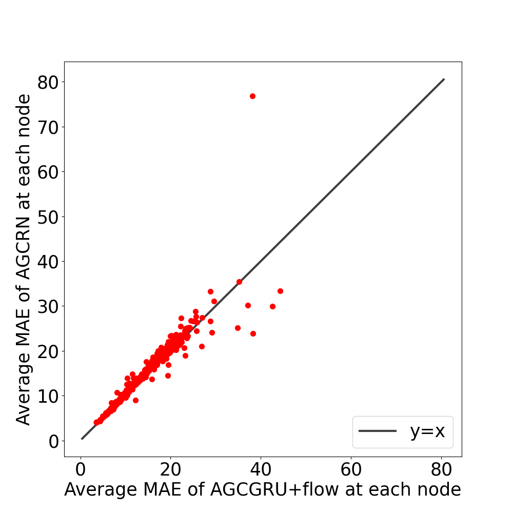
(a) PeMSD3

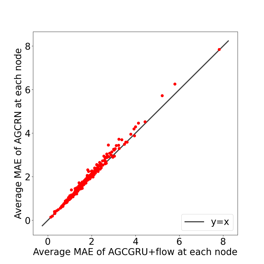
(b) PeMSD4

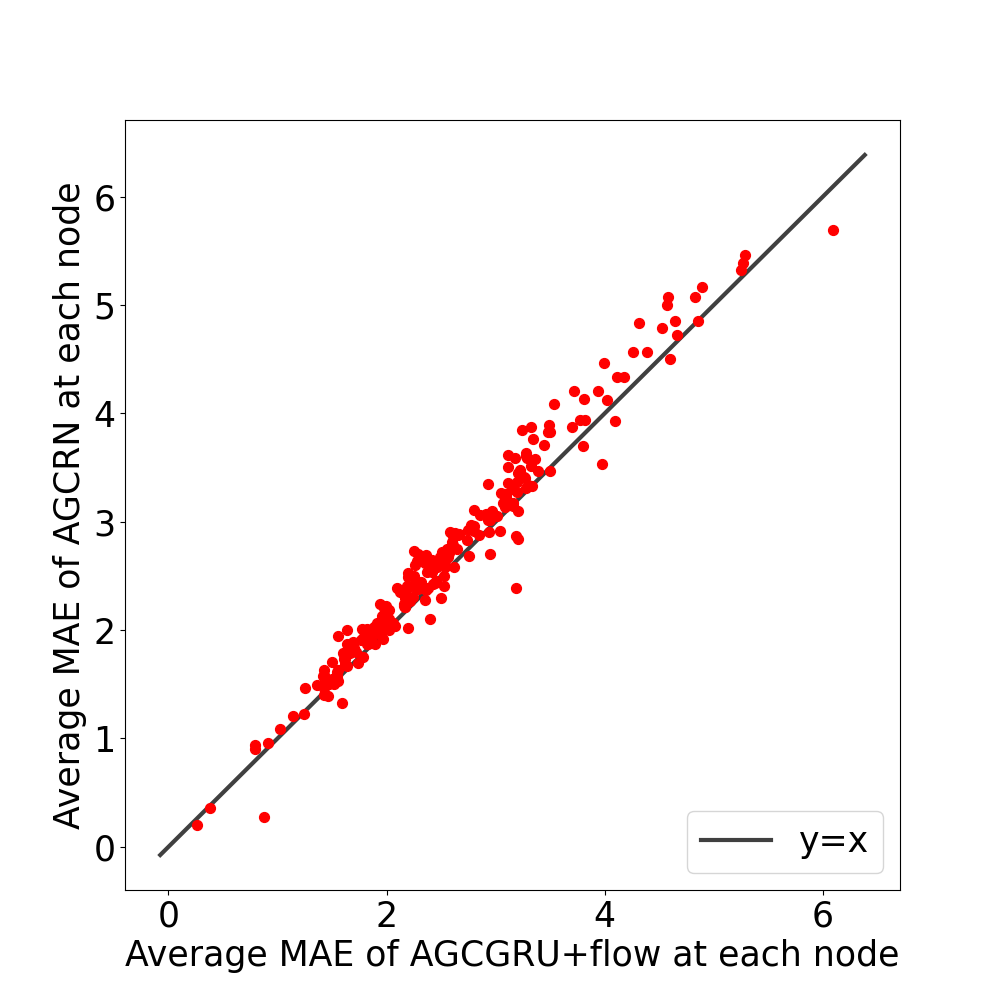
(c) PeMSD7

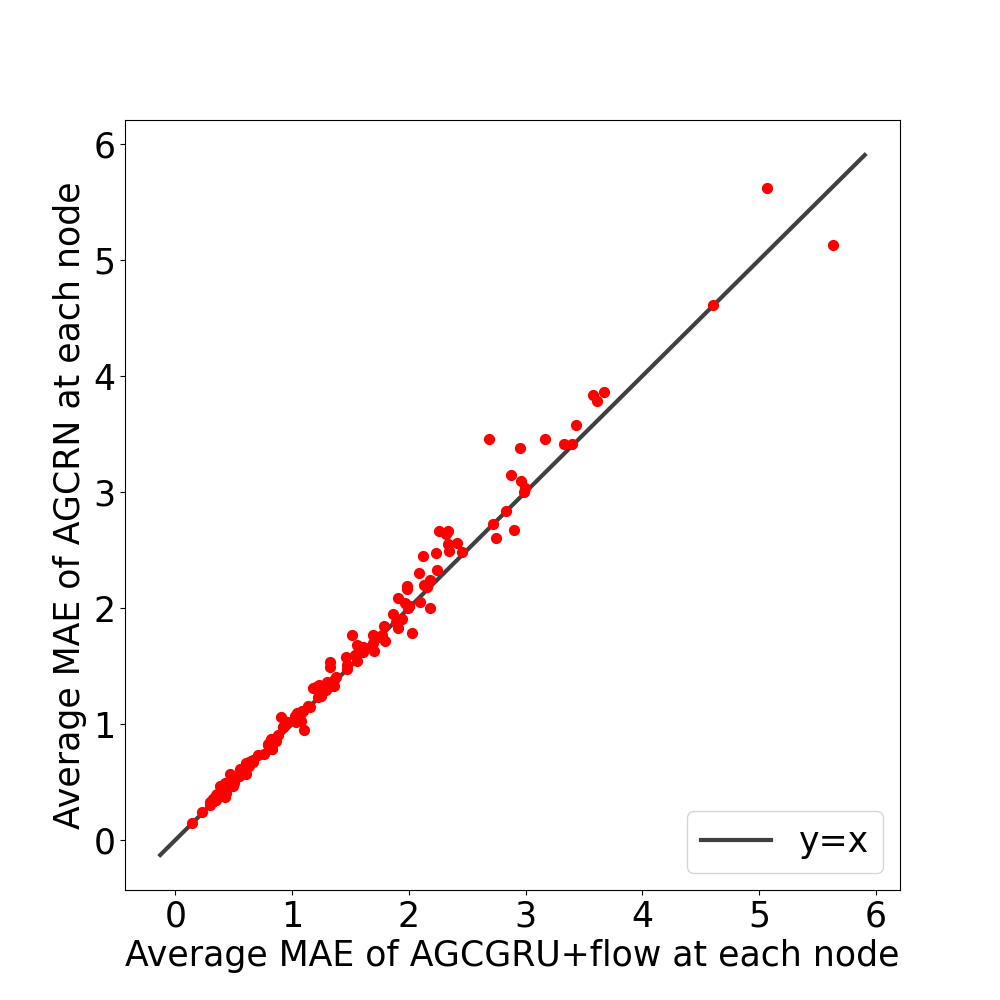
(d) PeMSD8

Figure 6: Scatter-plots of average MAE at each node for AGCGRU+flow v.s. that of AGCRN on PeMS datasets. The AGCGRU+flow has lower average MAE compared to AGCRN at most of the nodes for all four datasets.

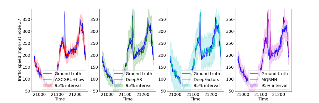
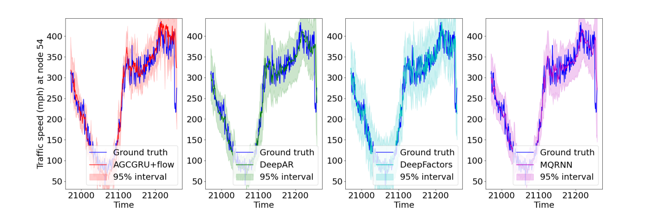
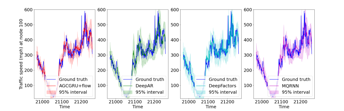
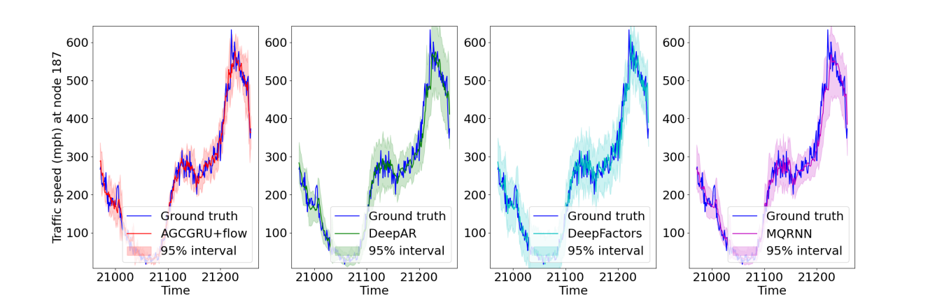
Figure 7: 15 minutes ahead predictions from the probabilistic forecasting algorithms with confidence intervals at nodes 37, 54, 100, and 187 of PeMSD3 dataset for the first day in the test set. The proposed AGCGRU+flow algorithm provides tighter confidence interval than its competitors in most cases, which leads to lower quantile error.

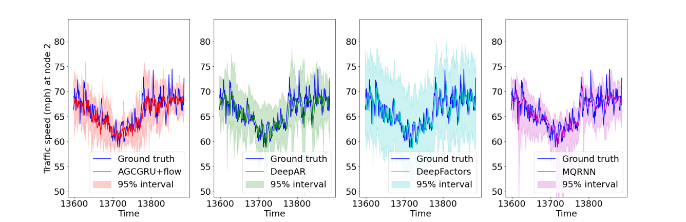
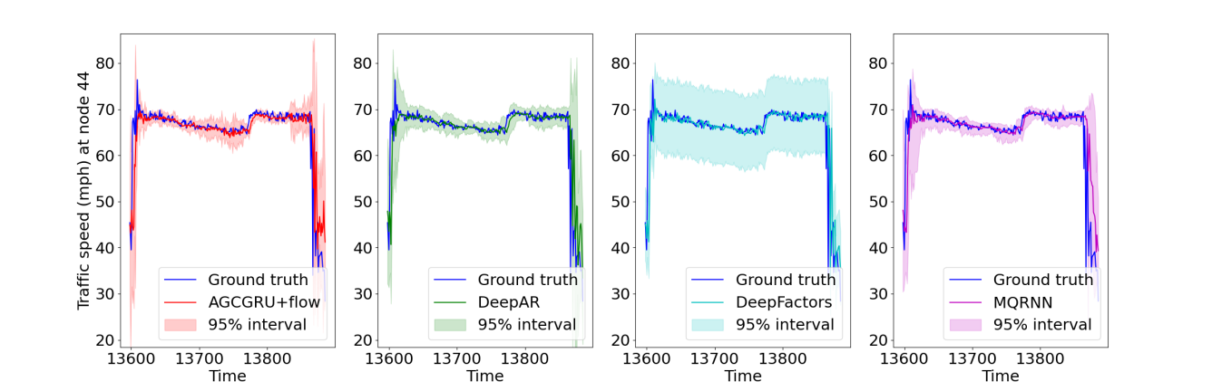
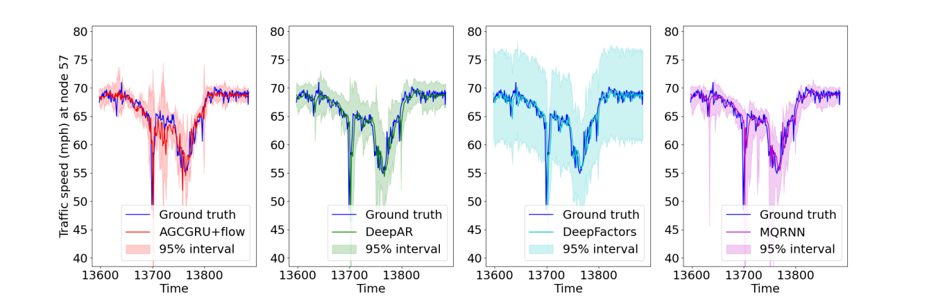
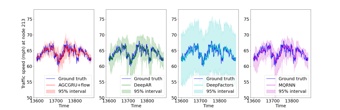
Figure 8: 15 minutes ahead predictions from the probabilistic forecasting algorithms with confidence intervals at nodes 2, 44, 57, and 213 of PeMSD4 dataset for the first day in the test set. The proposed AGCGRU+flow algorithm provides tighter confidence interval than its competitors in most cases, which leads to lower quantile error.

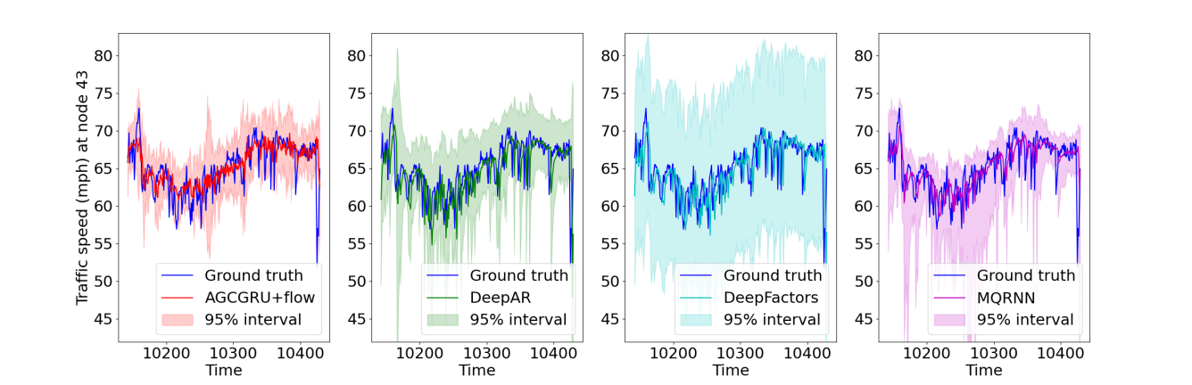
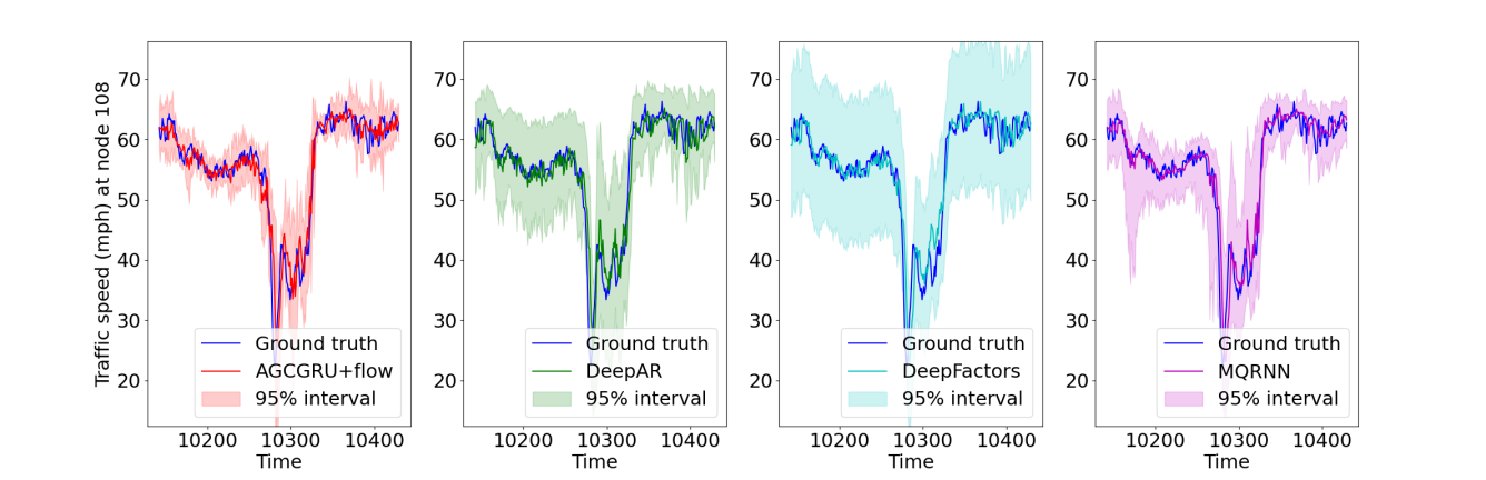
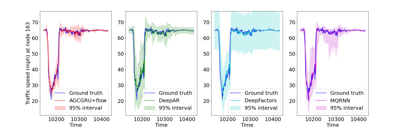
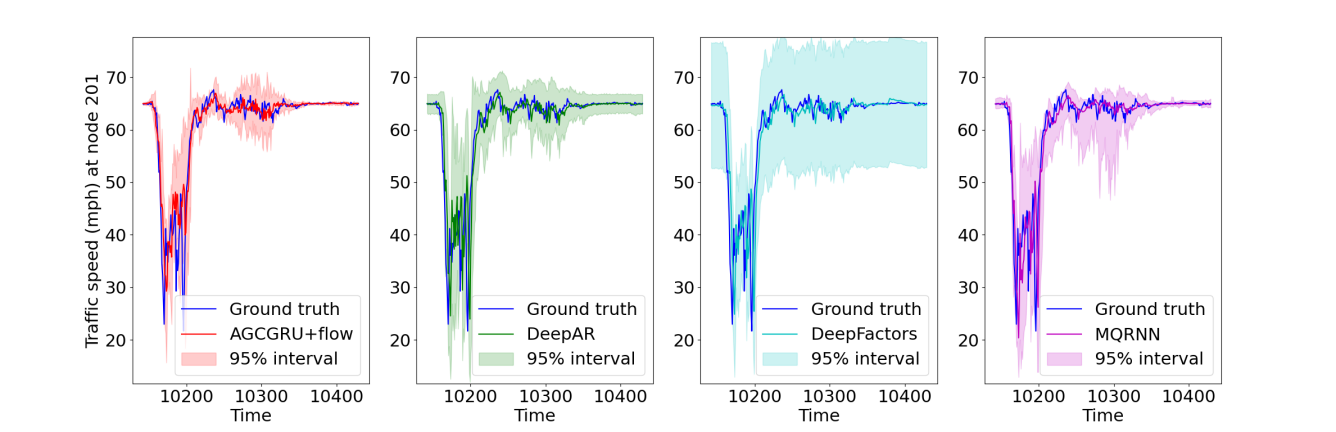
Figure 9: 15 minutes ahead predictions from the probabilistic forecasting algorithms with confidence intervals at nodes 43, 108, 163, and 201 of PeMSD7 dataset for the first day in the test set. The proposed AGCGRU+flow algorithm provides tighter confidence interval than its competitors in most cases, which leads to lower quantile error.

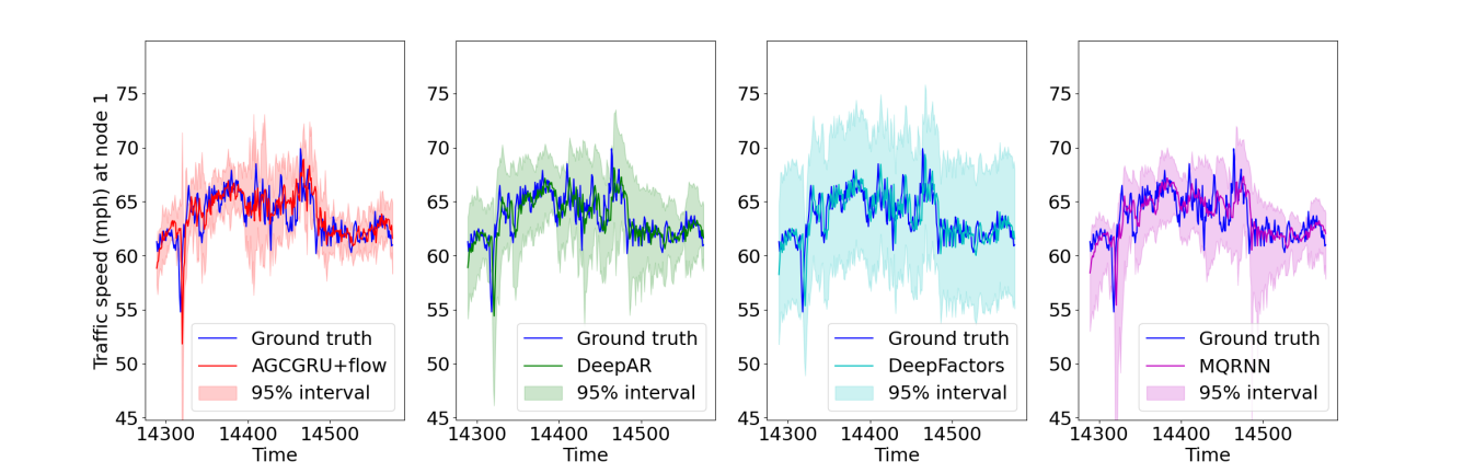
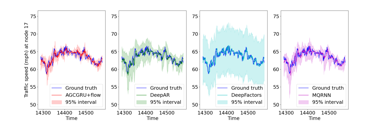
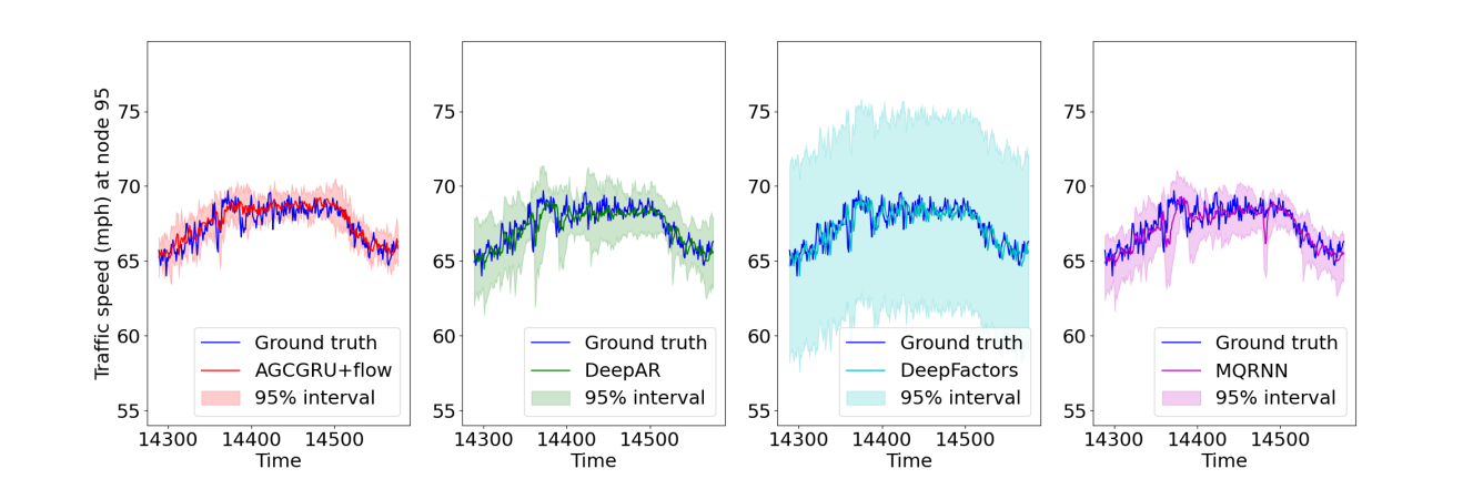
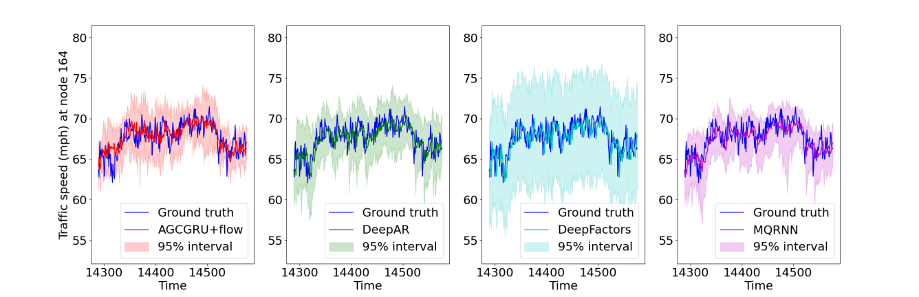
Figure 10: 15 minutes ahead predictions from the probabilistic forecasting algorithms with confidence intervals at nodes 1, 17, 95, and 164 of PeMSD8 dataset for the first day in the test set. The proposed AGCGRU+flow algorithm provides tighter confidence interval than its competitors in most cases, which leads to lower quantile error.

Table 14: Average MAE, MAPE, and RMSE for PeMSD3, PeMSD4, PeMSD7, and PeMSD8 for 15/30/45/60 minutes horizons for AGCGRU+flow and AGCGRU+BPF. Lower numbers are better.

Algorithm	PeMSD3 (15/ 30/ 45/ 60 min)
	MAE	MAPE(%)	RMSE
AGCGRU+flow	13.79/14.84/15.58/16.06	14.01/14.75/15.34/15.80	22.08/24.26/25.55/26.43
AGCGRU+BPF	14.19/15.13/15.85/16.35	14.21/14.86/15.40/15.82	25.69/27.38/28.51/29.26
Algorithm	PeMSD4 (15/ 30/ 45/ 60 min)
	MAE	MAPE(%)	RMSE
AGCGRU+flow	1.35/1.63/1.78/1.88	2.67/3.44/3.87/4.16	2.88/3.77/4.20/4.46
AGCGRU+BPF	1.36/1.65/1.80/1.90	2.71/3.46/3.90/4.18	2.91/3.81/4.25/4.52
Algorithm	PeMSD7 (15/ 30/ 45/ 60 min)
	MAE	MAPE(%)	RMSE
AGCGRU+flow	2.15/2.70/2.99/3.19	5.13/6.75/7.61/8.18	4.11/5.46/6.12/6.54
AGCGRU+BPF	2.19/2.73/2.99/3.17	5.27/6.86/7.69/8.21	4.18/5.52/6.16/6.53
Algorithm	PeMSD8 (15/ 30/ 45/ 60 min)
	MAE	MAPE(%)	RMSE
AGCGRU+flow	1.13/1.37/1.49/1.57	2.30/3.01/3.40/3.65	2.59/3.45/3.85/4.09
AGCGRU+BPF	1.18/1.41/1.52/1.59	2.47/3.13/3.50/3.74	2.69/3.53/3.92/4.15

Table 15: Average CRPS, P10QL, and P90QL for PeMSD3, PeMSD4, PeMSD7, and PeMSD8 for 15/30/45/60 minutes horizons for AGCGRU+flow and AGCGRU+BPF. Lower numbers are better.

Algorithm	PeMSD3 (15/ 30/ 45/ 60 min)
	CRPS	P10QL(%)	P90QL(%)
AGCGRU+flow	10.53/11.39/12.03/12.47	4.01/4.44/4.76/4.97	4.06/4.38/4.63/4.82
AGCGRU+BPF	11.32/11.94/12.55/12.92	4.36/4.66/4.98/5.13	4.39/4.65/4.88/5.07
Algorithm	PeMSD4 (15/ 30/ 45/ 60 min)
	CRPS	P10QL(%)	P90QL(%)
AGCGRU+flow	1.08/1.32/1.46/1.56	1.28/1.62/1.82/1.97	1.05/1.26/1.37/1.45
AGCGRU+BPF	1.10/1.32/1.45/1.54	1.29/1.60/1.79/1.92	1.06/1.26/1.37/1.45
Algorithm	PeMSD7 (15/ 30/ 45/ 60 min)
	CRPS	P10QL(%)	P90QL(%)
AGCGRU+flow	1.73/2.18/2.43/2.58	2.27/2.97/3.36/3.60	1.83/2.25/2.48/2.62
AGCGRU+BPF	1.79/2.24/2.49/2.66	2.35/3.02/3.40/3.67	1.86/2.29/2.53/2.69
Algorithm	PeMSD8 (15/ 30/ 45/ 60 min)
	CRPS	P10QL(%)	P90QL(%)
AGCGRU+flow	0.90/1.10/1.20/1.28	1.10/1.43/1.61/1.73	0.87/1.01/1.09/1.14
AGCGRU+BPF	0.96/1.13/1.22/1.28	1.19/1.47/1.63/1.74	0.91/1.03/1.09/1.13

12.2 Detailed results for comparison with particle filter

In Table 4 of the main paper, we compare the average MAE and average CRPS of the proposed AGCGRU+flow with a Bootstrap Particle Filter (BPF) (Gordon et al., 1993) based approach. Tables 14 and 15 provide the detailed comparison both in terms of point forecasting and probabilistic forecasting metrics. We observe that the proposed AGCGRU+flow algorithm outperforms the particle filter based approach in most cases.

12.3 Effect of number of particles

For this experiment, we consider three different settings with varying number of particles $N_{p}=1/10/50$ for testing. The model is trained using 1 particle in each case. From Table 16, we observe that increasing the number of particles cannot improve the point forecasting accuracy significantly, whereas the results in Table 17 show that characterization of the prediction uncertainty is improved as more particles are used to form the approximate posterior distribution of the forecasts.

Table 16: Average MAE, MAPE, and RMSE for PeMSD3, PeMSD4, PeMSD7, and PeMSD8 for 15/30/45/60 minutes horizons for AGCGRU+flow with different number of particles. Lower numbers are better.

Algorithm	PeMSD3 (15/ 30/ 45/ 60 min)
	MAE	MAPE(%)	RMSE
AGCGRU+flow ($N_{p}=1$)	13.82/14.87/15.60/16.08	14.04/14.78/15.36/15.82	22.33/24.41/25.70/26.54
AGCGRU+flow ($N_{p}=10$)	13.79/14.84/15.58/16.06	14.01/14.75/15.34/15.80	22.08/24.26/25.55/26.43
AGCGRU+flow ($N_{p}=50$)	13.79/14.84/15.58/16.06	14.01/14.74/15.33/15.79	22.02/24.20/25.55/26.42
Algorithm	PeMSD4 (15/ 30/ 45/ 60 min)
	MAE	MAPE(%)	RMSE
AGCGRU+flow ($N_{p}=1$)	1.35/1.63/1.78/1.88	2.68/3.45/3.89/4.18	2.89/3.78/4.22/4.47
AGCGRU+flow ($N_{p}=10$)	1.35/1.63/1.78/1.88	2.67/3.44/3.87/4.16	2.88/3.77/4.20/4.46
AGCGRU+flow ($N_{p}=50$)	1.35/1.63/1.78/1.88	2.67/3.44/3.87/4.16	2.88/3.77/4.20/4.45
Algorithm	PeMSD7 (15/ 30/ 45/ 60 min)
	MAE	MAPE(%)	RMSE
AGCGRU+flow ($N_{p}=1$)	2.16/2.71/3.00/3.20	5.14/6.77/7.63/8.20	4.12/5.47/6.14/6.56
AGCGRU+flow ($N_{p}=10$)	2.15/2.70/2.99/3.19	5.13/6.75/7.61/8.18	4.11/5.46/6.12/6.54
AGCGRU+flow ($N_{p}=50$)	2.15/2.70/2.99/3.19	5.12/6.75/7.61/8.18	4.11/5.46/6.12/6.54
Algorithm	PeMSD8 (15/ 30/ 45/ 60 min)
	MAE	MAPE(%)	RMSE
AGCGRU+flow ($N_{p}=1$)	1.14/1.38/1.50/1.57	2.31/3.02/3.41/3.67	2.60/3.46/3.87/4.11
AGCGRU+flow ($N_{p}=10$)	1.13/1.37/1.49/1.57	2.30/3.01/3.40/3.65	2.59/3.45/3.85/4.09
AGCGRU+flow ($N_{p}=50$)	1.13/1.37/1.49/1.57	2.30/3.01/3.40/3.65	2.59/3.44/3.85/4.09

Table 17: Average CRPS, P10QL, and P90QL for PeMSD3, PeMSD4, PeMSD7, and PeMSD8 for 15/30/45/60 minutes horizons for AGCGRU+flow with different number of particles. Lower numbers are better.

Algorithm	PeMSD3 (15/ 30/ 45/ 60 min)
	CRPS	P10QL(%)	P90QL(%)
AGCGRU+flow ($N_{p}=1$)	19.34/20.44/21.24/21.80	11.79/12.80/13.46/13.91	10.46/10.72/10.98/11.18
AGCGRU+flow ($N_{p}=10$)	10.53/11.39/12.03/12.47	4.01/4.44/4.76/4.97	4.06/4.38/4.63/4.82
AGCGRU+flow ($N_{p}=50$)	10.02/10.86/11.49/11.92	3.67/4.05/4.33/4.53	3.83/4.15/4.41/4.59
Algorithm	PeMSD4 (15/ 30/ 45/ 60 min)
	CRPS	P10QL(%)	P90QL(%)
AGCGRU+flow ($N_{p}=1$)	1.95/2.34/2.58/2.73	3.11/3.75/4.16/4.47	3.00/3.59/3.92/4.10
AGCGRU+flow ($N_{p}=10$)	1.08/1.32/1.46/1.56	1.28/1.62/1.82/1.97	1.05/1.26/1.37/1.45
AGCGRU+flow ($N_{p}=50$)	1.03/1.26/1.40/1.49	1.21/1.54/1.73/1.87	0.98/1.17/1.27/1.35
Algorithm	PeMSD7 (15/ 30/ 45/ 60 min)
	CRPS	P10QL(%)	P90QL(%)
AGCGRU+flow ($N_{p}=1$)	3.18/3.95/4.35/4.61	5.57/6.96/7.67/8.15	5.38/6.63/7.29/7.69
AGCGRU+flow ($N_{p}=10$)	1.73/2.18/2.43/2.58	2.27/2.97/3.36/3.60	1.83/2.25/2.48/2.62
AGCGRU+flow ($N_{p}=50$)	1.64/2.09/2.32/2.47	2.16/2.83/3.20/3.44	1.71/2.10/2.31/2.45
Algorithm	PeMSD8 (15/ 30/ 45/ 60 min)
	CRPS	P10QL(%)	P90QL(%)
AGCGRU+flow ($N_{p}=1$)	1.63/1.90/2.07/2.18	2.73/3.28/3.63/3.87	2.38/2.68/2.86/2.98
AGCGRU+flow ($N_{p}=10$)	0.90/1.10/1.20/1.28	1.10/1.43/1.61/1.73	0.87/1.01/1.09/1.14
AGCGRU+flow ($N_{p}=50$)	0.86/1.05/1.16/1.22	1.04/1.35/1.52/1.63	0.83/0.95/1.03/1.08

12.4 Effect of different learnable noise variance at each node

In this experiment, we compare the proposed state-space model with different learnable noise variance at each node (parameterized by the softplus function in eq. (9) in the main paper with fixed and uniform noise standard deviation $\gamma=0.01/0.05/0.10$ at all nodes. Other hyper-parameters and the training setup remain unchanged. The results in Table 18 demonstrate that the learnable noise variance approach is not particularly beneficial in comparison to a uniform, fixed variance approach in most cases. However, we note that the probabilistic metrics reported in Table 19 are the lowest for the learnable noise variance model in all cases. This suggests that different time-series in these road traffic datasets have different degrees of uncertainty which cannot be effectively modelled by the uniform, fixed noise variance approach.

Table 18: Average MAE, MAPE, and RMSE for PeMSD3, PeMSD4, PeMSD7, and PeMSD8 for 15/30/45/60 minutes horizons for AGCGRU+flow with learnable and fixed noise variance settings. The best result in each column is shown in bold. Lower numbers are better.

Algorithm	PeMSD3 (15/ 30/ 45/ 60 min)
	MAE	MAPE(%)	RMSE
AGCGRU+flow (learnable)	13.79/14.84/15.58/16.06	14.01/14.75/15.34/15.80	22.08/24.26/25.55/26.43
AGCGRU+flow ($\gamma=0.01$)	13.68/14.75/15.49/16.02	14.57/15.37/16.02/16.57	21.74/23.95/25.27/26.21
AGCGRU+flow ($\gamma=0.05$)	13.96/15.05/15.76/16.25	15.87/16.66/17.23/17.62	22.08/24.33/25.64/26.54
AGCGRU+flow ($\gamma=0.10$)	13.86/14.91/15.68/16.17	14.42/15.20/15.87/16.39	22.04/24.25/25.60/26.41
Algorithm	PeMSD4 (15/ 30/ 45/ 60 min)
	MAE	MAPE(%)	RMSE
AGCGRU+flow (learnable)	1.35/1.63/1.78/1.88	2.67/3.44/3.87/4.16	2.88/3.77/4.20/4.46
AGCGRU+flow ($\gamma=0.01$)	1.35/1.63/1.79/1.89	2.68/3.45/3.89/4.20	2.88/3.77/4.20/4.47
AGCGRU+flow ($\gamma=0.05$)	1.36/1.65/1.80/1.91	2.69/3.47/3.91/4.21	2.88/3.76/4.20/4.46
AGCGRU+flow ($\gamma=0.10$)	1.36/1.65/1.80/1.90	2.70/3.47/3.89/4.18	2.92/3.81/4.24/4.49
Algorithm	PeMSD7 (15/ 30/ 45/ 60 min)
	MAE	MAPE(%)	RMSE
AGCGRU+flow (learnable)	2.15/2.70/2.99/3.19	5.13/6.75/7.61/8.18	4.11/5.46/6.12/6.54
AGCGRU+flow ($\gamma=0.01$)	2.14/2.69/2.98/3.16	5.07/6.66/7.47/8.00	4.10/5.43/6.09/6.49
AGCGRU+flow ($\gamma=0.05$)	2.16/2.71/3.00/3.20	5.13/6.74/7.61/8.19	4.09/5.41/6.06/6.48
AGCGRU+flow ($\gamma=0.10$)	2.16/2.73/3.01/3.20	5.15/6.77/7.62/8.15	4.12/5.48/6.15/6.54
Algorithm	PeMSD8 (15/ 30/ 45/ 60 min)
	MAE	MAPE(%)	RMSE
AGCGRU+flow (learnable)	1.13/1.37/1.49/1.57	2.30/3.01/3.40/3.65	2.59/3.45/3.85/4.09
AGCGRU+flow ($\gamma=0.01$)	1.13/1.37/1.49/1.57	2.31/3.03/3.44/3.71	2.60/3.43/3.84/4.09
AGCGRU+flow ($\gamma=0.05$)	1.13/1.37/1.49/1.57	2.26/2.95/3.35/3.62	2.53/3.34/3.75/4.01
AGCGRU+flow ($\gamma=0.10$)	1.13/1.38/1.51/1.60	2.31/3.04/3.49/3.80	2.57/3.41/3.86/4.14

Table 19: Average CRPS, P10QL, and P90QL for PeMSD3, PeMSD4, PeMSD7, and PeMSD8 for 15/30/45/60 minutes horizons for AGCGRU+flow with learnable and fixed noise variance settings. The best result in each column is shown in bold. Lower numbers are better.

Algorithm	PeMSD3 (15/ 30/ 45/ 60 min)
	CRPS	P10QL(%)	P90QL(%)
AGCGRU+flow (learnable)	10.53/11.39/12.03/12.47	4.01/4.44/4.76/4.97	4.06/4.38/4.63/4.82
AGCGRU+flow ($\gamma=0.01$)	12.83/13.90/14.63/15.17	7.26/8.10/8.46/8.77	6.68/7.08/7.55/7.86
AGCGRU+flow ($\gamma=0.05$)	11.58/12.61/13.28/13.74	5.78/6.52/6.99/7.25	5.14/5.54/5.81/6.06
AGCGRU+flow ($\gamma=0.10$)	13.14/14.18/14.95/15.43	7.79/8.57/9.22/9.53	6.64/7.05/7.28/7.53
Algorithm	PeMSD4 (15/ 30/ 45/ 60 min)
	CRPS	P10QL(%)	P90QL(%)
AGCGRU+flow (learnable)	1.08/1.32/1.46/1.56	1.28/1.62/1.82/1.97	1.05/1.26/1.37/1.45
AGCGRU+flow ($\gamma=0.01$)	1.28/1.55/1.70/1.81	2.09/2.58/2.87/3.08	1.74/2.08/2.26/2.38
AGCGRU+flow ($\gamma=0.05$)	1.19/1.47/1.62/1.72	1.82/2.30/2.57/2.77	1.48/1.84/2.04/2.15
AGCGRU+flow ($\gamma=0.10$)	1.32/1.60/1.75/1.85	2.19/2.68/2.95/3.15	1.84/2.23/2.43/2.54
Algorithm	PeMSD7 (15/ 30/ 45/ 60 min)
	CRPS	P10QL(%)	P90QL(%)
AGCGRU+flow (learnable)	1.73/2.18/2.43/2.58	2.27/2.97/3.36/3.60	1.83/2.25/2.48/2.62
AGCGRU+flow ($\gamma=0.01$)	2.02/2.55/2.82/3.01	3.59/4.57/5.05/5.35	3.00/3.77/4.22/4.54
AGCGRU+flow ($\gamma=0.05$)	1.90/2.42/2.70/2.90	3.18/4.20/4.76/5.15	2.56/3.27/3.65/3.91
AGCGRU+flow ($\gamma=0.10$)	2.09/2.65/2.94/3.12	3.80/4.87/5.41/5.77	3.18/4.04/4.47/4.73
Algorithm	PeMSD8 (15/ 30/ 45/ 60 min)
	CRPS	P10QL(%)	P90QL(%)
AGCGRU+flow (learnable)	0.90/1.10/1.20/1.28	1.10/1.43/1.61/1.73	0.87/1.01/1.09/1.14
AGCGRU+flow ($\gamma=0.01$)	1.07/1.29/1.41/1.49	1.81/2.29/2.56/2.75	1.35/1.57/1.67/1.73
AGCGRU+flow ($\gamma=0.05$)	1.00/1.23/1.35/1.43	1.58/2.04/2.31/2.50	1.21/1.43/1.52/1.58
AGCGRU+flow ($\gamma=0.10$)	1.10/1.34/1.47/1.56	1.88/2.41/2.72/2.93	1.47/1.71/1.81/1.87

Table 20: Average MAE, MAPE, and RMSE for PeMSD3, PeMSD4, PeMSD7, and PeMSD8 for 15/30/45/60 minutes horizons for the proposed flow based approach and deterministic encoder-decoder models. Lower numbers are better.

Algorithm	PeMSD3 (15/ 30/ 45/ 60 min)
	MAE	MAPE(%)	RMSE
AGCGRU+flow	13.79/14.84/15.58/16.06	14.01/14.75/15.34/15.80	22.08/24.26/25.55/26.43
FC-AGCGRU	13.96/15.37/16.52/17.45	14.26/15.61/16.69/17.37	25.28/27.43/29.09/30.43
DCGRU+flow	14.48/15.67/16.52/17.36	15.06/16.06/16.91/17.84	23.86/26.12/27.54/28.76
FC-DCGRU	14.42/15.87/17.10/18.29	14.57/15.78/16.87/17.95	24.33/27.05/28.99/30.76
GRU+flow	14.40/16.10/17.63/19.18	14.56/15.99/17.33/18.89	23.06/26.15/28.64/30.97
FC-GRU	15.82/18.37/20.61/22.93	15.87/18.82/21.32/23.75	25.85/30.09/33.37/36.94
Algorithm	PeMSD4 (15/ 30/ 45/ 60 min)
	MAE	MAPE(%)	RMSE
AGCGRU+flow	1.35/1.63/1.78/1.88	2.67/3.44/3.87/4.16	2.88/3.77/4.20/4.46
FC-AGCGRU	1.37/1.74/2.00/2.20	2.69/3.67/4.41/5.00	2.92/3.96/4.62/5.09
DCGRU+flow	1.38/1.71/1.92/2.08	2.72/3.63/4.23/4.67	2.93/3.93/4.49/4.87
FC-DCGRU	1.38/1.78/2.06/2.29	2.69/3.72/4.51/5.16	2.95/4.09/4.81/5.34
GRU+flow	1.37/1.76/2.02/2.23	2.70/3.74/4.52/5.15	2.95/4.05/4.74/5.23
FC-GRU	1.46/1.91/2.25/2.54	2.84/3.97/4.88/5.66	3.10/4.35/5.20/5.85
Algorithm	PeMSD7 (15/ 30/ 45/ 60 min)
	MAE	MAPE(%)	RMSE
AGCGRU+flow	2.15/2.70/2.99/3.19	5.13/6.75/7.61/8.18	4.11/5.46/6.12/6.54
FC-AGCGRU	2.21/2.99/3.56/4.05	5.18/7.39/9.12/10.64	4.18/5.88/7.03/7.94
DCGRU+flow	2.19/2.87/3.29/3.61	5.16/7.17/8.48/9.42	4.16/5.66/6.54/7.14
FC-DCGRU	2.23/3.06/3.67/4.18	5.19/7.50/9.31/10.90	4.26/6.05/7.28/8.24
GRU+flow	2.24/3.02/3.55/3.96	5.27/7.58/9.30/10.60	4.28/5.97/7.00/7.73
FC-GRU	2.41/3.40/4.17/4.84	5.60/8.27/10.47/12.40	4.56/6.68/8.17/9.34
Algorithm	PeMSD8 (15/ 30/ 45/ 60 min)
	MAE	MAPE(%)	RMSE
AGCGRU+flow	1.13/1.37/1.49/1.57	2.30/3.01/3.40/3.65	2.59/3.45/3.85/4.09
FC-AGCGRU	1.16/1.48/1.70/1.87	2.30/3.17/3.78/4.25	2.58/3.53/4.12/4.54
DCGRU+flow	1.17/1.44/1.58/1.70	2.35/3.12/3.57/3.87	2.64/3.54/4.00/4.28
FC-DCGRU	1.16/1.49/1.70/1.87	2.25/3.16/3.85/4.37	2.54/3.49/4.08/4.49
GRU+flow	1.12/1.41/1.59/1.74	2.17/2.94/3.50/3.92	2.55/3.47/4.02/4.40
FC-GRU	1.20/1.56/1.81/2.02	2.29/3.09/3.70/4.22	2.63/3.61/4.24/4.73

Table 21: Average MAE, MAPE, and RMSE for PeMSD3, PeMSD4, PeMSD7, and PeMSD8 for 15/30/45/60 minutes horizons for AGCRN-ensemble, GMAN-ensemble, and AGCGRU+flow. The best and the second best results in each column are shown in bold and marked with underline respectively. Lower numbers are better.

Algorithm	PeMSD3 (15/ 30/ 45/ 60 min)
	MAE	MAPE(%)	RMSE
AGCRN-ensemble	14.21/15.12/15.73/16.22	13.91/14.56/14.93/15.38	25.49/27.16/28.20/28.90
GMAN-ensemble	14.48/15.20/15.90/16.66	15.01/15.64/16.41/17.36	23.96/25.20/26.31/27.44
AGCGRU+flow	13.79/14.84/15.58/16.06	14.01/14.75/15.34/15.80	22.08/24.26/25.55/26.43
Algorithm	PeMSD4 (15/ 30/ 45/ 60 min)
	MAE	MAPE(%)	RMSE
AGCRN-ensemble	1.35/1.61/1.76/1.91	2.75/3.40/3.79/4.17	2.89/3.65/4.09/4.47
GMAN-ensemble	1.33/1.57/1.72/1.84	2.64/3.27/3.70/4.04	2.89/3.62/4.04/4.33
AGCGRU+flow	1.35/1.63/1.78/1.88	2.67/3.44/3.87/4.16	2.88/3.77/4.20/4.46
Algorithm	PeMSD7 (15/ 30/ 45/ 60 min)
	MAE	MAPE(%)	RMSE
AGCRN-ensemble	2.17/2.69/2.95/3.20	5.25/6.75/7.55/8.22	4.09/5.29/5.94/6.45
GMAN-ensemble	2.42/2.80/3.08/3.35	6.08/7.18/8.00/8.74	4.68/5.54/6.08/6.51
AGCGRU+flow	2.15/2.70/2.99/3.19	5.13/6.75/7.61/8.18	4.11/5.46/6.12/6.54
Algorithm	PeMSD8 (15/ 30/ 45/ 60 min)
	MAE	MAPE(%)	RMSE
AGCRN-ensemble	1.19/1.36/1.46/1.58	2.67/3.10/3.38/3.68	2.88/3.41/3.76/4.06
GMAN-ensemble	1.13/1.28/1.39/1.49	2.37/2.78/3.10/3.37	2.71/3.25/3.61/3.87
AGCGRU+flow	1.13/1.37/1.49/1.57	2.30/3.01/3.40/3.65	2.59/3.45/3.85/4.09

Table 22: Average CRPS, P10QL, and P90QL for PeMSD3, PeMSD4, PeMSD7, and PeMSD8 for 15/30/45/60 minutes horizons for AGCRN-ensemble, GMAN-ensemble, and AGCGRU+flow. The best and the second best results in each column are shown in bold and marked with underline respectively. Lower numbers are better.

Algorithm	PeMSD3 (15/ 30/ 45/ 60 min)
	CRPS	P10QL(%)	P90QL(%)
AGCRN-ensemble	12.64/13.44/13.96/14.27	6.90/7.40/7.54/7.53	6.10/6.43/6.79/6.96
GMAN-ensemble	12.79/13.49/14.13/14.77	7.17/7.67/8.08/8.45	5.86/6.16/6.44/6.68
AGCGRU+flow	10.53/11.39/12.03/12.47	4.01/4.44/4.76/4.97	4.06/4.38/4.63/4.82
Algorithm	PeMSD4 (15/ 30/ 45/ 60 min)
	CRPS	P10QL(%)	P90QL(%)
AGCRN-ensemble	1.20/1.44/1.56/1.68	1.82/2.21/2.39/2.57	1.53/1.82/1.93/2.08
GMAN-ensemble	1.16/1.38/1.51/1.62	1.73/2.11/2.35/2.54	1.45/1.70/1.82/1.92
AGCGRU+flow	1.08/1.32/1.46/1.56	1.28/1.62/1.82/1.97	1.05/1.26/1.37/1.45
Algorithm	PeMSD7 (15/ 30/ 45/ 60 min)
	CRPS	P10QL(%)	P90QL(%)
AGCRN-ensemble	1.90/2.39/2.60/2.81	3.22/4.15/4.55/4.89	2.55/3.19/3.35/3.58
GMAN-ensemble	1.96/2.31/2.53/2.73	3.16/3.83/4.23/4.53	2.20/2.59/2.81/3.00
AGCGRU+flow	1.73/2.18/2.43/2.58	2.27/2.97/3.36/3.60	1.83/2.25/2.48/2.62
Algorithm	PeMSD8 (15/ 30/ 45/ 60 min)
	CRPS	P10QL(%)	P90QL(%)
AGCRN-ensemble	1.03/1.20/1.28/1.38	1.63/1.97/2.14/2.34	1.18/1.34/1.39/1.48
GMAN-ensemble	0.95/1.10/1.19/1.28	1.40/1.68/1.88/2.04	1.12/1.26/1.34/1.41
AGCGRU+flow	0.90/1.10/1.20/1.28	1.10/1.43/1.61/1.73	0.87/1.01/1.09/1.14

12.5 Detailed comparison with deterministic encoder-decoder models

In Table 2 of the main paper, we compare the average MAE of the proposed flow based approaches with those of the deterministic encoder-decoder based sequence to sequence prediction models for three different RNN architectures. In Table 20, we report the MAPE and RMSE, in addition to the MAE. We see that the particle flow based RNN models outperform the corresponding deterministic encoder-decoder models in most cases.

12.6 Detailed results for comparison to ensembles

In Table 5 of the main paper, we compare the average CRPS of the proposed AGCGRU+flow algorithm with ensembles of AGCRN and GAMN. From Table 21, we observe that our approach is comparable or slightly worse compared to the ensembles in terms of the MAE, MAPE and RMSE of the point forecasts. However, the proposed AGCGRU+flow shows better characterization of the prediction uncertainty compared to the ensemble methods in almost all cases, as shown in Table 22.

12.7 Comparison with a Variational Inference (VI) based approach

Although there is no directly applicable baseline forecasting method in the literature that incorporates VI, RNNs, and GNNs, we can derive a variational approach using equivalent GNN-RNN architectures and compare it to the particle flow approach. We wish to approximate $p_{\Theta}(\mathbf{y}_{P+1:P+Q}|\mathbf{y}_{1:P},\mathbf{z}_{1:P+Q})$. So, the ELBO is defined as follows:

$$\mathcal{L}(\Theta,\Omega) =\mathbb{E}_{q_{\Omega}}\Bigg{[}\log p_{\Theta}(\mathbf{y}_{P+1:P+Q},\mathbf{x}_{1:P}|\mathbf{y}_{1:P},\mathbf{z}_{1:P+Q})\,$$

$$\qquad-\log q_{\Omega}(\mathbf{x}_{1:P}|\mathbf{y}_{1:P+Q},\mathbf{z}_{1:P+Q})\Bigg{]}\,.$$ (35)

Now, we approximate

$$p_{\Theta}(\mathbf{y}_{P+1:P+Q},\mathbf{x}_{1:P}|\mathbf{y}_{1:P},\mathbf{z}_{1:P+Q})\,$$

$$=\int\prod_{t=P+1}^{P+Q}\Big{(}p_{\phi,\gamma}(\mathbf{y}_{t}|\mathbf{x}_{t},\mathbf{z}_{t})\,$$

$$\qquad\qquad\qquad\quad p_{\psi,\sigma}(\mathbf{x}_{t}|\mathbf{x}_{t-1},\mathbf{y}_{t-1},\mathbf{z}_{t})\Big{)}d\mathbf{x}_{P+1:P+Q}\,,$$

$$\approx\prod_{t=P+1}^{P+Q}\Bigg{[}\frac{1}{N_{p}}\sum_{j=1}^{N_{p}}p_{\phi,\gamma}(\mathbf{y}_{t}|\mathbf{x}_{t}^{j},\mathbf{z}_{t})\Bigg{]}\,,$$ (36)

where, in the decoder, we first sample $\mathbf{x}_{t}^{j}$ from $p_{\psi,\sigma}(\mathbf{x}_{t}|\mathbf{x}_{t-1}^{j},\mathbf{y}_{t-1}^{j},\mathbf{z}_{t})$ (for $t>P+1$) or from $p_{\psi,\sigma}(\mathbf{x}_{t}|\mathbf{x}_{t-1}^{j},\mathbf{y}_{t-1},\mathbf{z}_{t})$ (for $t=P+1$) for $1\leqslant j\leqslant N_{p}$ and then sample $\mathbf{y}_{t}^{j}$ from $p_{\phi,\gamma}(\mathbf{y}_{t}|\mathbf{x}_{t}^{j},\mathbf{z}_{t})$ for $1\leqslant j\leqslant N_{p}$ to form the MC approximation. This decoder is initialized using the output of the encoder, i.e., we sample $\mathbf{x}_{1:P}^{j}$ from the inference distribution $q_{\Omega}(\mathbf{x}_{1:P}|\mathbf{y}_{1:P+Q},\mathbf{z}_{1:P+Q})$ for $1\leqslant j\leqslant N_{p}$, which is assumed to be factorized as follows:

$$q_{\Omega}(\mathbf{x}_{1:P}|\mathbf{y}_{1:P+Q},\mathbf{z}_{1:P+Q})\,$$

$$\qquad=q_{\Omega}(\mathbf{x}_{1:P}|\mathbf{y}_{1:P},\mathbf{z}_{1:P})\,,$$

$$\qquad=q_{1}(\mathbf{x}_{1},\mathbf{z}_{1},\rho)\prod_{t=2}^{P}q_{\psi^{\prime},\sigma^{\prime}}(\mathbf{x}_{t}|\mathbf{x}_{t-1},\mathbf{y}_{t-1},\mathbf{z}_{t})\,.$$ (37)

Here, we set $q_{1}(\mathbf{x}_{1},\mathbf{z}_{1},\rho)=p_{1}(\mathbf{x}_{1},\mathbf{z}_{1},\rho)$ for simplicity and we use the same RNN architecture (i.e. AGCGRU) for $q_{\psi^{\prime},\sigma^{\prime}}$ and $p_{\psi,\sigma}$.

Experimental details : We treat $\rho$, $\sigma$ and $\sigma^{\prime}$ as hyperparameters and set $\rho=1$ and $\sigma=\sigma^{\prime}=0$. This implies that $q_{\psi^{\prime},\sigma^{\prime}}$ is a Dirac-delta function and the maximization of ELBO (in eq. (35)) using SGD (SGVI) amounts to mimization of the same cost function as defined in eq. (14) in the main paper. The only difference is that now a) we have two separate AGCGRUs for encoder and decoder and b) there is no particle flow in the forward pass. We call this model AGCGRU+VI and compare it to AGCGRU+flow. The other hyperparameters are set to the same values as for the AGCGRU+flow algorithm. From Table 23, we observe that for comparable RNN architectures, the flow based algorithm significantly outperforms the variational inference based approach in the point forecasting task. The results in Table 24 indicate that in the probabilistic forecasting task, both particle flow and VI approaches show comparable performance despite AGCGRU+flow having approximately half of the learnable parameters of the AGCGRU+VI model.

Table 23: Average MAE, MAPE, and RMSE for PeMSD3, PeMSD4, PeMSD7, and PeMSD8 for 15/30/45/60 minutes horizons for AGCGRU+flow and AGCGRU+VI. Lower numbers are better.

Algorithm	PeMSD3 (15/ 30/ 45/ 60 min)
	MAE	MAPE(%)	RMSE
AGCGRU+flow	13.79/14.84/15.58/16.06	14.01/14.75/15.34/15.80	22.08/24.26/25.55/26.43
AGCGRU+VI	15.08/16.10/16.83/17.53	15.26/16.10/16.74/17.43	26.17/28.02/29.13/30.17
Algorithm	PeMSD4 (15/ 30/ 45/ 60 min)
	MAE	MAPE(%)	RMSE
AGCGRU+flow	1.35/1.63/1.78/1.88	2.67/3.44/3.87/4.16	2.88/3.77/4.20/4.46
AGCGRU+VI	1.46/1.76/1.94/2.06	2.94/3.73/4.20/4.52	2.97/3.78/4.22/4.48
Algorithm	PeMSD7 (15/ 30/ 45/ 60 min)
	MAE	MAPE(%)	RMSE
AGCGRU+flow	2.15/2.70/2.99/3.19	5.13/6.75/7.61/8.18	4.11/5.46/6.12/6.54
AGCGRU+VI	2.33/2.92/3.23/3.45	5.59/7.26/8.16/8.78	4.22/5.48/6.10/6.50
Algorithm	PeMSD8 (15/ 30/ 45/ 60 min)
	MAE	MAPE(%)	RMSE
AGCGRU+flow	1.13/1.37/1.49/1.57	2.30/3.01/3.40/3.65	2.59/3.45/3.85/4.09
AGCGRU+VI	1.29/1.52/1.65/1.74	2.94/3.51/3.86/4.10	2.96/3.59/3.94/4.17

Table 24: Average CRPS, P10QL, and P90QL for PeMSD3, PeMSD4, PeMSD7, and PeMSD8 for 15/30/45/60 minutes horizons for AGCGRU+flow and AGCGRU+VI. Lower numbers are better.

Algorithm	PeMSD3 (15/ 30/ 45/ 60 min)
	CRPS	P10QL(%)	P90QL(%)
AGCGRU+flow	10.53/11.39/12.03/12.47	4.01/4.44/4.76/4.97	4.06/4.38/4.63/4.82
AGCGRU+VI	11.00/11.80/12.38/12.94	4.14/4.53/4.82/5.10	4.27/4.58/4.81/5.02
Algorithm	PeMSD4 (15/ 30/ 45/ 60 min)
	CRPS	P10QL(%)	P90QL(%)
AGCGRU+flow	1.08/1.32/1.46/1.56	1.28/1.62/1.82/1.97	1.05/1.26/1.37/1.45
AGCGRU+VI	1.08/1.31/1.45/1.54	1.26/1.59/1.79/1.93	1.04/1.25/1.36/1.45
Algorithm	PeMSD7 (15/ 30/ 45/ 60 min)
	CRPS	P10QL(%)	P90QL(%)
AGCGRU+flow	1.73/2.18/2.43/2.58	2.27/2.97/3.36/3.60	1.83/2.25/2.48/2.62
AGCGRU+VI	1.72/2.18/2.42/2.60	2.25/2.97/3.39/3.66	1.80/2.24/2.47/2.63
Algorithm	PeMSD8 (15/ 30/ 45/ 60 min)
	CRPS	P10QL(%)	P90QL(%)
AGCGRU+flow	0.90/1.10/1.20/1.28	1.10/1.43/1.61/1.73	0.87/1.01/1.09/1.14
AGCGRU+VI	0.95/1.13/1.24/1.31	1.15/1.44/1.62/1.76	0.90/1.03/1.10/1.15

12.8 Comparison of execution time, GPU memory usage and model size

Table 25 summarizes the run time, GPU usage during training, and the size of the learned model for AGCRN-ensemble, GMAN-ensemble, and the proposed AGCGRU+flow for the four PeMS datasets. We observe that if we choose the ensemble size so that the algorithms have an approximately equal execution time, then the model-size of the ensemble algorithms are comparable to our approach as well. However, our method requires more GPU memory compared to the ensembles during training because of the particle flow in the forward pass.

Table 25: Execution time, memory consumption (during training) and model size for AGCRN-ensemble, GMAN-ensemble and AGCGRU+flow for the four PeMS datasets. Lower numbers are better.

Algorithm	Execution time (minutes)
	PEMS03	PEMS04	PEMS07	PEMS08
AGCRN-ensemble	369	243	183	224
GMAN-ensemble	444	224	195	185
AGCGRU+flow	325	205	154	177
Algorithm	GPU memory (GB)
	PEMS03	PEMS04	PEMS07	PEMS08
AGCRN-ensemble	6.55	5.19	4.09	3.47
GMAN-ensemble	15.45	9.45	8.46	4.45
AGCGRU+flow	25.27	18.76	12.45	8.45
Algorithm	Model Size (MB)
	PEMS03	PEMS04	PEMS07	PEMS08
AGCRN-ensemble	11.52	11.52	11.45	11.45
GMAN-ensemble	9.54	9.51	9.45	9.35
AGCGRU+flow	12.88	12.86	12.86	12.85

References

- Bai et al. (2019) Bai, L., Yao, L., Kanhere, S., Wang, X., and Sheng, Q. STG2Seq: Spatial-temporal graph to sequence model for multi-step passenger demand forecasting. In Proc. Int. Joint Conf. Artificial Intell., pp. 1981–1987, 2019.
- Bai et al. (2020) Bai, L., Yao, L., Li, C., Wang, X., and Wang, C. Adaptive graph convolutional recurrent network for traffic forecasting. In Proc. Adv. Neural Info. Process. Systems, 2020.
- Bao et al. (2017) Bao, W., Yue, J., and Rao, Y. A deep learning framework for financial time series using stacked autoencoders and long-short term memory. PloS One, 12(7), 2017.
- Bayer & Osendorfer (2014) Bayer, J. and Osendorfer, C. Learning stochastic recurrent networks. arXiv e-prints: arXiv:1411.7610, 2014.
- Bengio et al. (2015) Bengio, S., Vinyals, O., Jaitly, N., and Shazeer, N. Scheduled sampling for sequence prediction with recurrent neural networks. In Proc. Adv. Neural Info. Process. Systems, volume 1, pp. 1171–1179, 2015.
- Bengtsson et al. (2008) Bengtsson, T., Bickel, P., and Li, B. Curse-of-dimensionality revisited: Collapse of the particle filter in very large scale systems. In Probability and Statistics: Essays in Honor of David A. Freedman, volume 2, pp. 316–334. Institute of Mathematical Statistics, Beachwood, OH, USA, Apr. 2008.
- Beskos et al. (2014) Beskos, A., Crisan, D., and Jasra, A. On the stability of sequential Monte Carlo methods in high dimensions. Ann. Appl. Prob., 24(4):1396–1445, 2014.
- Boulanger-Lewandowski et al. (2012) Boulanger-Lewandowski, N., Bengio, Y., and Vincent, P. Modeling temporal dependencies in high-dimensional sequences: Application to polyphonic music generation and transcription. arXiv preprint arXiv:1206.6392, 2012.
- Chang et al. (2018) Chang, Y.-Y., Sun, F.-Y., Wu, Y.-H., and Lin, S.-D. A memory-network based solution for multivariate time-series forecasting. arXiv preprint arXiv:1809.02105, 2018.
- Chen et al. (2000) Chen, C., Petty, K., and Skabardonis, A. Freeway performance measurement system: Mining loop detector data. Transport. Research Record, 1748, Jan. 2000.
- Chen et al. (2019a) Chen, C., Li, K., Teo, S. G., Zou, X., Wang, K., Wang, J., and Zeng, Z. Gated residual recurrent graph neural networks for traffic prediction. In Proc. AAAI Conf. Artificial Intell., pp. 485–492, 2019a.
- Chen et al. (2018) Chen, R. T., Rubanova, Y., Bettencourt, J., and Duvenaud, D. Neural ordinary differential equations. In Proc. Adv. Neural Info. Process. Systems, 2018.
- Chen et al. (2020) Chen, W., Chen, L., Xie, Y., Cao, W., Gao, Y., and Feng, X. Multi-range attentive bicomponent graph convolutional network for traffic forecasting. In Proc. AAAI Conf. Artificial Intell., pp. 3529–3536, 2020.
- Chen et al. (2019b) Chen, X., Dai, H., and Song, L. Particle flow Bayes’ rule. In Proc. Int. Conf. Machine Learning, pp. 1022–1031, 2019b.
- Choi et al. (2011) Choi, S., Willett, P., Daum, F., and Huang, J. Discussion and application of the homotopy filter. In Proc. SPIE Conf. Signal Process., Sensor Fusion, Target Recog., pp. 805021, Orlando, FL, USA, May 2011.
- Chun-Hsin et al. (2004) Chun-Hsin, W., Jan-Ming, H., and T., L. D. Travel-time prediction with support vector regression. IEEE Trans. Intell. Transport. Systems, 5(4):276–281, 2004.
- Chung et al. (2014) Chung, J., Gulcehre, C., Cho, K., and Bengio, Y. Empirical evaluation of gated recurrent neural networks on sequence modeling. In Proc. Workshop on Deep Learning, Adv. Neural Info. Process. Systems, 2014.
- Chung et al. (2015) Chung, J., Kastner, K., Dinh, L., Goel, K., Courville, A. C., and Bengio, Y. A recurrent latent variable model for sequential data. In Proc. Adv. Neural Info. Process. Systems, pp. 2980–2988, 2015.
- Daum & Huang (2007) Daum, F. and Huang, J. Nonlinear filters with log-homotopy. In Proc. SPIE Signal and Data Process. Small Targets, pp. 669918, San Diego, CA, USA, Sep. 2007.
- Daum & Huang (2014) Daum, F. and Huang, J. Seven dubious methods to mitigate stiffness in particle flow with non-zero diffusion for nonlinear filters, Bayesian decisions, and transport. In Proc. SPIE Conf. Signal Process., Sensor Fusion, Target Recog., pp. 90920C, Baltimore, MD, USA, May 2014.
- Daum et al. (2010) Daum, F., Huang, J., and Noushin, A. Exact particle flow for nonlinear filters. In Proc. SPIE Conf. Signal Process., Sensor Fusion, Target Recog., pp. 769704, Orlando, FL, USA, Apr. 2010.
- Daum et al. (2017) Daum, F., Huang, J., and Noushin, A. Generalized Gromov method for stochastic particle flow filters. In Proc. SPIE Conf. Signal Process., Sensor Fusion, Target Recog., pp. 102000I, Anaheim, CA, USA, May 2017.
- de Bézenac et al. (2020) de Bézenac, E., Rangapuram, S. S., Benidis, K., Bohlke-Schneider, M., Kurle, R., Stella, L., Hasson, H., Gallinari, P., and Januschowski, T. Normalizing kalman filters for multivariate time series analysis. In Proc. Adv. Neural Info. Process. Systems, volume 33, 2020.
- Defferrard et al. (2016) Defferrard, M., Bresson, X., and Vandergheynst, P. Convolutional neural networks on graphs with fast localized spectral filtering. In Proc. Adv. Neural Inf. Proc. Systems, pp. 3844–3852, 2016.
- Ding & Coates (2012) Ding, T. and Coates, M. J. Implementation of the daum-huang exact-flow particle filter. In Proc. IEEE Statist. Signal Process. Workshop (SSP), pp. 257–260, Ann Arbor, MI, USA, Aug. 2012.
- Doerr et al. (2018) Doerr, A., Daniel, C., Schiegg, M., Nguyen-Tuong, D., Schaal, S., Toussaint, M., and Trimpe, S. Probabilistic recurrent state-space models. arXiv preprint arXiv:1801.10395, 2018.
- Doucet & Johansen (2009) Doucet, A. and Johansen, A. M. A tutorial on particle filtering and smoothing: Fifteen years later. In The Oxford Handbook of Nonlinear Filtering, chapter 24, pp. 656–704. Oxford University Press, Oxford, UK, 2009.
- Dua & Graff (2017) Dua, D. and Graff, C. UCI machine learning repository, 2017. URL http://archive.ics.uci.edu/ml.
- Fraccaro et al. (2016) Fraccaro, M., Sønderby, S. K., Paquet, U., and Winther, O. Sequential neural models with stochastic layers. arXiv eprints, arXiv:1605.07571, 2016.
- Fraccaro et al. (2017) Fraccaro, M., Kamronn, S., Paquet, U., and Winther, O. A disentangled recognition and nonlinear dynamics model for unsupervised learning. In Proc. Adv. Neural Info. Process. Systems, 2017.
- Gammelli & Rodrigues (2020) Gammelli, D. and Rodrigues, F. Recurrent flow networks: A recurrent latent variable model for spatio-temporal density modelling. arXiv eprints, arXiv:2006.05256, 2020.
- Gneiting & Raftery (2007) Gneiting, T. and Raftery, A. E. Strictly proper scoring rules, prediction, and estimation. J. Amer. Statist. Association, 102(477):359–378, 2007.
- Gordon et al. (1993) Gordon, N., Salmond, D., and Smith, A. Novel approach to nonlinear/non-Gaussian Bayesian state estimation. IEE Proc. F Radar and Signal Process., 140:107–113, Apr. 1993.
- Gu et al. (2015) Gu, S. S., Ghahramani, Z., and Turner, R. E. Neural adaptive sequential monte carlo. In Proc. Adv. Neural Info. Process. Systems, volume 28, pp. 2629–2637, 2015.
- Guo et al. (2019) Guo, S., Lin, Y., Feng, N., Song, C., and Wan, H. Attention based spatial-temporal graph convolutional networks for traffic flow forecasting. In Proc. AAAI Conf. Artificial Intell., 2019.
- Guo & Lin (2018) Guo, T. and Lin, T. Multi-variable LSTM neural network for autoregressive exogenous model. arXiv preprint arXiv:1806.06384, 2018.
- Hamilton (1994) Hamilton, J. D. Time Series Analysis. Princeton University Press, 1 edition, January 1994.
- Huang et al. (2020) Huang, R., Huang, C., Liu, Y., Dai, G., and Kong, W. LSGCN: Long short-term traffic prediction with graph convolutional networks. In Proc. Int. Joint Conf. Artificial Intell., pp. 2355–2361, 7 2020.
- Huang et al. (2019) Huang, Y., Weng, Y., Yu, S., and Chen, X. Diffusion convolutional recurrent neural network with rank influence learning for traffic forecasting. In Proc. IEEE Int. Conf. Big Data Science And Engineering, pp. 678–685, Aug 2019.
- Karkus et al. (2018) Karkus, P., Hsu, D., and Lee, W. S. Particle filter networks with application to visual localization. In Proc. Conf. Robot Learning, pp. 169–178, 2018.
- Karl et al. (2016) Karl, M., Soelch, M., Bayer, J., and Van der Smagt, P. Deep variational Bayes filters: Unsupervised learning of state space models from raw data. In Proc. Int. Conf. Learning Rep., 2016.
- Kipf & Welling (2017) Kipf, T. and Welling, M. Semi-supervised classification with graph convolutional networks. In Proc. Int. Conf. Learning Rep., 2017.
- Kobyzev et al. (2020) Kobyzev, I., Prince, S., and Brubaker, M. Normalizing flows: An introduction and review of current methods. IEEE Trans. Pattern Analysis and Machine Intell., 2020.
- Kumar et al. (2019) Kumar, M., Babaeizadeh, M., Erhan, D., Finn, C., Levine, S., Dinh, L., and Kingma, D. Videoflow: A flow-based generative model for video. arXiv preprint arXiv:1903.01434, 2(5), 2019.
- Kurle et al. (2020) Kurle, R., Rangapuram, S. S., de Bézenac, E., Günnemann, S., and Gasthaus, J. Deep Rao-Blackwellised particle filters for time series forecasting. In Proc. Adv. Neural Info. Process. Systems, 2020.
- Lai et al. (2018) Lai, G., Chang, W.-C., Yang, Y., and Liu, H. Modeling long-and short-term temporal patterns with deep neural networks. In Proc. ACM Int. Conf. Research & Development in Info. Retrieval, pp. 95–104, 2018.
- Le et al. (2017) Le, T. A., Igl, M., Rainforth, T., Jin, T., and Wood, F. Auto-encoding sequential Monte Carlo. arXiv preprint arXiv:1705.10306, 2017.
- Li et al. (2019) Li, L., Yan, J., Yang, X., and Jin, Y. Learning interpretable deep state space model for probabilistic time series forecasting. In Proc. Int. Joint Conf. on Artificial Intell., pp. 2901–2908, 2019.
- Li & Coates (2017) Li, Y. and Coates, M. Particle filtering with invertible particle flow. IEEE Trans. Signal Process., 65(15):4102–4116, Aug. 2017.
- Li et al. (2018) Li, Y., Yu, R., Shahabi, C., and Liu, Y. Diffusion Convolutional Recurrent Neural Network: Data-Driven Traffic Forecasting. In Proc. Int. Conf. Learning Rep., 2018.
- Ma et al. (2020) Ma, X., Karkus, P., Hsu, D., and Lee, W. S. Particle filter recurrent neural networks. In Proc. AAAI Conf. Artificial Intell., pp. 5101–5108, 2020.
- Maddison et al. (2017) Maddison, C. J., Lawson, D., Tucker, G., Heess, N., Norouzi, M., Mnih, A., Doucet, A., and Teh, Y. W. Filtering variational objectives. In Proc. Adv. Neural Info. Process. Systems, 2017.
- Makridakis & Hibon (1997) Makridakis, S. and Hibon, M. Arma models and the box-jenkins methodology. J. Forecasting, 16(3):147–163, January 1997.
- Mattos et al. (2016) Mattos, C. L. C., Dai, Z., Damianou, A., Forth, J., Barreto, G. A., and Lawrence, N. D. Recurrent Gaussian processes. In Proc. Int. Conf. Learning Rep., 2016.
- Naesseth et al. (2018) Naesseth, C., Linderman, S., Ranganath, R., and Blei, D. Variational sequential Monte Carlo. In Proc. Int. Conf. Artificial Intell. and Statist., pp. 968–977, 2018.
- Oreshkin et al. (2020) Oreshkin, B. N., Carpov, D., Chapados, N., and Bengio, Y. N-BEATS: Neural basis expansion analysis for interpretable time series forecasting. In Proc. Int. Conf. Learning Rep., 2020.
- Oreshkin et al. (2021) Oreshkin, B. N., Amini, A., Coyle, L., and Coates, M. J. FC-GAGA: Fully Connected Gated Graph Architecture for spatio-temporal traffic forecasting. In Proc. AAAI Conf. Artificial Intell., Jan. 2021.
- Pan et al. (2019) Pan, Z., Liang, Y., Wang, W., Yu, Y., Zheng, Y., and Zhang, J. Urban traffic prediction from spatio-temporal data using deep meta learning. In Proc. ACM SIGKDD Int. Conf. Knowl. Discov. & Data Mining, pp. 1720–1730, 2019.
- Park et al. (2020) Park, C., Lee, C., Bahng, H., won, T., Kim, K., Jin, S., Ko, S., and Choo, J. ST-GRAT: A spatio-temporal graph attention network for traffic forecasting. In Proc. AAAI Conf. Artificial Intell., 2020.
- Qin et al. (2017) Qin, Y., Song, D., Chen, H., Cheng, W., Jiang, G., and Cottrell, G. W. A dual-stage attention-based recurrent neural network for time series prediction. In Proc. Int. Joint Conf. Artificial Intell., 2017.
- Rangapuram et al. (2018) Rangapuram, S. S., Seeger, M. W., Gasthaus, J., Stella, L., Wang, Y., and Januschowski, T. Deep state space models for time series forecasting. In Proc. Adv. Neural Info. Process. Systems, 2018.
- Rasul et al. (2021) Rasul, K., Sheikh, A.-S., Schuster, I., Bergmann, U., and Vollgraf, R. Multi-variate probabilistic time series forecasting via conditioned normalizing flows. In Proc. Int. Conf. Learning Rep., 2021.
- Salinas et al. (2019) Salinas, D., Bohlke-Schneider, M., Callot, L., Medico, R., and Gasthaus, J. High-dimensional multivariate forecasting with low-rank Gaussian copula processes. In Proc. Adv. Neural Info. Process. Systems, 2019.
- Salinas et al. (2020) Salinas, D., Flunkert, V., Gasthaus, J., and Januschowski, T. DeepAR: Probabilistic forecasting with autoregressive recurrent networks. Int. J. Forecasting, 36(3):1181 – 1191, 2020.
- Sen et al. (2019) Sen, R., Yu, H.-F., and Dhillon, I. S. Think globally, act locally: A deep neural network approach to high-dimensional time series forecasting. In Proc. Adv. Neural Info. Process. Systems, volume 32, pp. 4837–4846, 2019.
- Shi et al. (2020) Shi, X., Qi, H., Shen, Y., Wu, G., and Yin, B. A spatial-temporal attention approach for traffic prediction. IEEE Trans. Intell. Transport. Systems, pp. 1–10, Apr. 2020.
- Smyl (2020) Smyl, S. A hybrid method of exponential smoothing and recurrent neural networks for time series forecasting. Int. J. Forecasting, 36(1):75 – 85, 2020.
- Snyder et al. (2008) Snyder, C., Bengtsson, T., Bickel, P., and Anderson, J. Obstacles to high-dimensional particle filtering. Mon. Weather Rev., 136(12):4629–4640, Dec. 2008.
- Song et al. (2020) Song, C., Lin, Y., Guo, S., and Wan, H. Spatial-temporal synchronous graph convolutional networks: A new framework for spatial-temporal network data forecasting. In Proc. AAAI Conf. Artificial Intell., pp. 914–921, Apr. 2020.
- Sutskever et al. (2014) Sutskever, I., Vinyals, O., and Le, Q. V. Sequence to sequence learning with neural networks. In Proc. Adv. Neural Info. Process. Systems, volume 27, pp. 3104–3112, 2014.
- Wang et al. (2019) Wang, Y., Smola, A., Maddix, D., Gasthaus, J., Foster, D., and Januschowski, T. Deep factors for forecasting. In Proc. Int. Conf. Machine Learning, Long Beach, California, USA, Jun 2019.
- Wen et al. (2017) Wen, R., Torkkola, K., Narayanaswamy, B., and Madeka, D. A Multi-Horizon Quantile Recurrent Forecaster. arXiv e-prints, arXiv:1711.11053, 2017.
- Wu et al. (2019) Wu, Z., Pan, S., Long, G., Jiang, J., and Zhang, C. Graph wavenet for deep spatial-temporal graph modeling. In Proc. Int. Joint Conf. Artificial Intell., pp. 1907–1913, 2019.
- Wu et al. (2019) Wu, Z., Pan, S., Long, G., Jiang, J., and Zhang, C. Graph WaveNet for Deep Spatial-Temporal Graph Modeling. In Proc. Int. Joint Conf. Artificial Intell., 2019.
- Wu et al. (2020) Wu, Z., Pan, S., Long, G., Jiang, J., Chang, X., and Zhang, C. Connecting the dots: Multivariate time series forecasting with graph neural networks. In Proc. ACM SIGKDD Conf. Knowl. Discov. & Data Mining, pp. 753–763, 08 2020.
- Xu et al. (2020) Xu, M., Dai, W., Liu, C., Gao, X., Lin, W., Qi, G.-J., and Xiong, H. Spatial-temporal transformer networks for traffic flow forecasting. arXiv preprint arXiv:2001.02908, 2020.
- Yu et al. (2018) Yu, B., Yin, H., and Zhu, Z. Spatio-Temporal Graph Convolutional Networks: A Deep Learning Framework for Traffic Forecasting. In Proc. Int. Joint Conf. Artificial Intell., 2018.
- Yu et al. (2019) Yu, B., Li, M., Zhang, J., and Zhu, Z. 3d graph convolutional networks with temporal graphs: A spatial information free framework for traffic forecasting. arXiv preprint arXiv:1903.00919, 2019.
- Zhang et al. (2020) Zhang, Q., Chang, J., Meng, G., Xiang, S., and Pan, C. Spatio-temporal graph structure learning for traffic forecasting. In Proc. AAAI Conf. Artificial Intell., pp. 1177–1185, Apr. 2020.
- Zhao et al. (2019) Zhao, R., Wang, K., Su, H., and Ji, Q. Bayesian graph convolution lstm for skeleton based action recognition. In Pro. IEEE/CVF Int. Conf. Computer Vision, Oct. 2019.
- Zheng et al. (2020) Zheng, C., Fan, X., Wang, C., and Qi, J. GMAN: A Graph Multi-Attention Network for Traffic Prediction. In Proc. AAAI Conf. Artificial Intell., 2020.
- Zheng et al. (2017) Zheng, X., Zaheer, M., Ahmed, A., Wang, Y., Xing, E. P., and Smola, A. J. State space LSTM models with particle MCMC inference. arXiv e-prints: arxiv 1711.11179, 2017.