Scalable Variational Gaussian Processes via Harmonic Kernel Decomposition

Abstract

We introduce a new scalable variational Gaussian process approximation which provides a high fidelity approximation while retaining general applicability. We propose the harmonic kernel decomposition (HKD), which uses Fourier series to decompose a kernel as a sum of orthogonal kernels. Our variational approximation exploits this orthogonality to enable a large number of inducing points at a low computational cost. We demonstrate that, on a range of regression and classification problems, our approach can exploit input space symmetries such as translations and reflections, and it significantly outperforms standard variational methods in scalability and accuracy. Notably, our approach achieves state-of-the-art results on CIFAR-10 among pure GP models.

1 Introduction

Gaussian Processes (GPs) (Rasmussen & Williams, 2006) are flexible Bayesian nonparametric models which enable principled reasoning about distributions of functions and provide rigorous uncertainty estimates (Srinivas et al., 2010; Deisenroth & Rasmussen, 2011). Unfortunately, exact inference in GPs is impractical for large datasets because of the $\mathcal{O}(N^{3})$ computational cost (for a dataset of size $N$). To overcome the computational roadblocks, sparse Gaussian processes (Snelson & Ghahramani, 2006; Quinonero-Candela & Rasmussen, 2005) use $M$ inducing points to approximate the kernel function, reducing the computational cost to $\mathcal{O}(NM^{2}+M^{3})$. However, these approaches are prone to overfitting since all inducing points are hyperparameters. Sparse variational Gaussian Processes (SVGPs) (Titsias, 2009; Hensman et al., 2015) offer an effective protection against overfitting by framing a posterior approximation using the inducing points and optimizing them with variational inference. Still, the $\mathcal{O}(M^{3})$ complexity prevents SVGPs from scaling beyond a few thousand inducing points, creating difficulties in improving the quality of approximation.

Several approaches impose structure on the inducing points to increase the approximation capacity. Structured kernel interpolation (SKI) (Wilson & Nickisch, 2015; Wilson et al., 2015) approximates the kernel by placing inducing points over a Euclidean grid and exploiting fast structured matrix operations. SKI can use millions of inducing points, but is limited to low-dimensional problems because the grid size grows exponentially with the input dimension. Other approaches define approximate posteriors using multiple sets of inducing points. Cheng & Boots (2017); Salimbeni et al. (2018) propose to decouple the inducing points for modelling means and covariances, leading to a linear complexity with respect to the number of mean inducing points. SOLVE-GP (Shi et al., 2020) reformulates a GP as the sum of two orthogonal processes and uses distinct groups of inducing points for each; this has the benefit of improving the approximation at a lower cost than standard SVGPs.

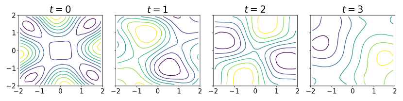
Figure 1: Visualizing the harmonic kernel decomposition. We decompose a $2$-dimensional RBF kernel as $k=\sum_{t=0}^{3}k_{t}$ using the symmetry group of $90^{\text{o}}$ rotations. We plot the real part of random functions sampled from each $\mathcal{GP}(0,k_{t})$. Notice that $\mathcal{GP}(0,k_{0})$ is invariant to $90^{\text{o}}$ rotations; $\mathcal{GP}(0,k_{1})$ takes opposite values under $180^{\text{o}}$ rotations; $\mathcal{GP}(0,k_{2})$ is invariant to $180^{\text{o}}$ rotations but has opposite values under $90^{\text{o}}$ rotations.

In this paper, we introduce a more scalable variational approximation for GPs via the proposed harmonic kernel decomposition (HKD), which decomposes the kernel as a sum of orthogonal kernels, $k(\mathbf{x},\mathbf{x}^{\prime})=\sum_{t=0}^{T-1}k_{t}(\mathbf{x},\mathbf{x}^{\prime})$, using Fourier series. The HKD reformulates the Gaussian process into an additive GP, where each subprocess models a Fourier component of the function (see Figure 1 for a visualization). We then propose the Harmonic Variational Gaussian Process (HVGP), which uses separate sets of inducing points for the subprocesses. Compared to a standard variational approximation, HVGPs allow us to use a large number of inducing points at a much lower computational cost. Moreover, HVGPs have an advantage over SKI in that they allow trainable inducing points. Finally, unlike the SOLVE-GP whose decomposition involves only two subprocesses, our HVGP is easily applicable to multiple subprocesses and can be computed efficiently with the discrete Fourier transform.

Empirically, we demonstrate the scalability and general applicability of HVGPs through a range of problems and models including using RBF kernels for modelling earth elevations and using convolutional kernels for image classification. In these experiments, HVGPs significantly outperform standard variational methods by exploiting the input-space symmetries such as translations and reflections. Our model can further exploit parallelism to achieve minimal wall-clock overhead when using 8 groups of inducing points. In CIFAR-10 classification, we show that our method can be integrated with deep convolutional structures to achieve state-of-the-art results for GPs.

2 Background

2.1 Discrete Fourier Transform

Fourier analysis (Baron Fourier, 1878) studies the representation of functions as sums or integrals of sinusoids. For an integrable function $f$ on $\mathbb{R}^{d}$, its Fourier transform is defined as

$$\hat{f}(\bm{\omega})=\int_{\mathbb{R}^{d}}e^{-2\pi i\bm{\omega}^{\top}\mathbf{x}}f(\mathbf{x})\,\mathrm{d}\mathbf{x},$$ (1)

where $\hat{f}(\bm{\omega})\in\mathbb{C}$. In kernel theory, Bochner’s Theorem (Bochner, 1959) is a seminal result that uses the Fourier transform to establish a bijection between stationary kernels and positive measures in the spectral domain.

Fourier analysis can be performed over finite sequences as well, via the discrete Fourier transform (DFT) (Cooley et al., 1969). Specifically, given a sequence $\mathbf{x}=[\mathbf{x}_{0},...,\mathbf{x}_{T-1}]^{\top}$​, DFT computes the sequence $\hat{\mathbf{x}}=[\hat{\mathbf{x}}_{0},...,\hat{\mathbf{x}}_{T-1}]^{\top}$​, with

$$\hat{\mathbf{x}}_{t}=\frac{1}{T}\sum_{s=0}^{T-1}\mathbf{x}_{s}e^{-i\frac{2\pi ts}{T}},\;t=0,...,T-1.$$ (2)

Let $\mathbf{F}:=[\frac{1}{T}e^{-i\frac{2\pi ts}{T}}]_{t,s=0}^{T-1}\in\mathbb{C}^{T\times T}$ denote the DFT matrix. The DFT can be represented in vector form as $\hat{\mathbf{x}}=\mathbf{F}\mathbf{x}$, which naturally leads to the inverse DFT: $\mathbf{x}=\mathbf{F}^{-1}\hat{\mathbf{x}}$.

More generally, if $\mathbf{X}\in\mathbb{C}^{T_{1}\times\cdots\times T_{k}}$ is a tensor, the multidimensional DFT computes the tensor $\hat{\mathbf{X}}\in\mathbb{C}^{T_{1}\times\cdots\times T_{k}}$,

$$\hat{\mathbf{X}}[t_{1},...,t_{k}]=\frac{1}{T}\sum_{s_{1},...,s_{k}}X[s_{1},...,s_{k}]\prod_{j=1}^{k}e^{-i\frac{2\pi t_{j}s_{j}}{T_{j}}},$$

where $T=\prod_{j}T_{j}$. The DFT matrix is then a tensor product of one-dimensional DFT matrices.

2.2 Gaussian Processes

Given an input domain $\mathcal{X}$, a mean function $m$, and a kernel function $k:\mathcal{X}\times\mathcal{X}\to\mathbb{R}$, the Gaussian process (Rasmussen & Williams, 2006) $\mathcal{GP}(m,k)$ is a distribution over functions $\mathcal{X}\to\mathbb{R}$. For any finite set $\{\mathbf{x}_{1},\mathbf{x}_{2},\dots,\mathbf{x}_{N}\}\subset\mathcal{X}$, the function values $\mathbf{f}=[f(\mathbf{x}_{1}),f(\mathbf{x}_{2}),...,f(\mathbf{x}_{N})]^{\top}$ have a multivariate Gaussian distribution:

$$\mathbf{f}\sim\mathcal{N}(m(\mathbf{X}),\mathbf{K}_{\mathbf{f}\mathbf{f}}),$$

where $m(\mathbf{X})=[m(\mathbf{x}_{1}),...,m(\mathbf{x}_{N})]^{\top}$​, and $\mathbf{K}_{\mathbf{f}\mathbf{f}}=[k(\mathbf{x}_{i},\mathbf{x}_{j})]_{i,j=1}^{N}$. For simplicity we assume $m(\cdot)=0$ throughout the paper. The observations $y$ are modeled with a density $p(y|f(\mathbf{x}))$, often taken to be Gaussian in the regression setting: $y=f(\mathbf{x})+\epsilon,\quad\epsilon\sim\mathcal{N}(0,\sigma^{2})$. Let $(\mathbf{X},\mathbf{y})$ be a training set of size $N$. The posterior distribution $p(\mathbf{f}^{\star}|\mathbf{y})$ under a Gaussian observation model is

$$\mathcal{N}(\mathbf{K}_{\star\mathbf{f}}(\mathbf{K}_{\mathbf{f}\mathbf{f}}+\sigma^{2}\mathbf{I})^{-1}\mathbf{y},\mathbf{K}_{\star\star}-\mathbf{K}_{\star\mathbf{f}}(\mathbf{K}_{\mathbf{f}\mathbf{f}}+\sigma^{2}\mathbf{I})^{-1}\mathbf{K}_{\mathbf{f}\star}),$$

where $\mathbf{f}^{\star}=f(\mathbf{X}^{\star})$ are function values at test locations. Unfortunately, computing the posterior mean and covariance requires inverting the kernel matrix, an $\mathcal{O}(N^{3})$ computation.

Sparse variational Gaussian processes (SVGPs) (Titsias, 2009; Hensman et al., 2013) use inducing points for scalable GP inference. Let $\mathbf{Z}=[\mathbf{z}_{1},...,\mathbf{z}_{M}]^{\top}\in\mathbb{R}^{M\times d}$ be $M$ inducing locations, and $\mathbf{u}=f(\mathbf{Z})$. SVGPs consider an augmented joint likelihood, $p(f(\cdot),\mathbf{u})=p(f(\cdot)|\mathbf{u})p(\mathbf{u})$, and a variational approximation $q(f(\cdot),\mathbf{u})=p(f(\cdot)|\mathbf{u})q(\mathbf{u})$, where $q(\mathbf{u})=\mathcal{N}(\bm{\mu},\mathbf{S})$ is a parameterized multivariate Gaussian with mean $\bm{\mu}$ and covariance $\mathbf{S}$. The variational approximation is optimized by maximizing the variational lower bound:

$$\mathcal{L}\vcentcolon=\mathbb{E}_{q(\mathbf{f},\mathbf{u})}[\log p(\mathbf{y}|\mathbf{f},\mathbf{X})]-\mathrm{KL}\left(q(\mathbf{u})||p(\mathbf{u})\right).$$ (3)

Since $\log p(\mathbf{y}|\mathbf{f},\mathbf{X})=\sum_{i=1}^{N}\log p(\mathbf{y}_{i}|f(\mathbf{x}_{i}))$ admits stochastic optimization, SVGPs reduce the computational cost to $\mathcal{O}(M^{3}+M^{2}B)$, where $B$ is the minibatch size.

3 Harmonic Kernel Decomposition

In this section, we introduce kernel Fourier series and use them to form the harmonic kernel decomposition. All proofs can be found in Section D.2.

3.1 Kernel Fourier Series

We first propose a general method for representing a kernel as a sum of functions. The idea is based on the DFT (see Sec. 2.1). Let $k:\mathcal{X}\times\mathcal{X}\to\mathbb{C}$ be a positive definite kernel. To apply the DFT, we fix the first input $\mathbf{x}$, and construct a finite sequence of kernel values using a transformation $G:\mathcal{X}\to\mathcal{X}$ that applies to the second input:

$$[k(\mathbf{x},G^{0}(\mathbf{x}^{\prime})),k(\mathbf{x},G^{1}(\mathbf{x}^{\prime})),...,k(\mathbf{x},G^{T-1}(\mathbf{x}^{\prime}))],$$ (4)

where $G^{0}(\mathbf{x}):=\mathbf{x}$ and $G^{t}:=G\circ G^{t-1}$. Note that in signal processing, the sequence under DFT usually contains equally-spaced samples along the time domain. Here, we adopt a more general form by using $G$ to exploit symmetries in the input domain.

Definition 3.1 (Kernel Fourier Series).

We define $T$ complex-valued functions $k_{t}:\mathcal{X}\times\mathcal{X}\to\mathbb{C}$, $t=0,~{}\dots,~{}T-1$ using the DFT of the sequence 4:

$$k_{t}(\mathbf{x},\mathbf{x}^{\prime})=\sum_{s=0}^{T-1}\mathbf{F}_{t,s}k(\mathbf{x},G^{s}(\mathbf{x}^{\prime})),$$ (5)

where $\mathbf{F}$ is the DFT matrix (see Sec. 2.1). The kernel Fourier series of $k(\mathbf{x},G^{s}(\mathbf{x}^{\prime}))$ is given by the inverse DFT:

$$k(\mathbf{x},G^{s}(\mathbf{x}^{\prime}))=\sum_{t=0}^{T-1}\mathbf{F}_{s,t}^{-1}k_{t}(\mathbf{x},\mathbf{x}^{\prime}).$$ (6)

The inverse DFT matrix is $\mathbf{F}^{-1}=T\mathbf{F}^{H}$, where $\cdot^{H}$ is the conjugate transpose.

Given the positive definiteness of $k$, it is tempting to ask whether $k_{t}$ is also a (complex-valued) kernel. In the next section, we will study the conditions when this holds and use it to form an orthogonal kernel decomposition.

3.2 Harmonic Kernel Decomposition

We first introduce the following definitions.

Definition 3.2 ($T$-Cyclic Transformation).

A function $G:\mathcal{X}\to\mathcal{X}$ is $T$-cyclic if $T$ is the smallest integer such that,

$$\forall\mathbf{x}\in\mathcal{X},\;G^{T}(\mathbf{x})\vcentcolon=\overbrace{G\circ\cdots\circ G}^{T}(\mathbf{x})=\mathbf{x}.$$ (7)

In group theory, $\{G^{0},G^{1},\dots,G^{T-1}\}$ forms a cyclic group of order $T$, and $G$ is the generator of this group. Interestingly, given a $T$-cyclic $G$, multiplying $k_{t}$ with $e^{i\frac{2\pi t}{T}}$ corresponds to a shift by $G$ in the second input.

Proposition 3.3 (Shift).

For any $0\leq t\leq T-1$,

$$k_{t}(\mathbf{x},G(\mathbf{x}^{\prime}))=e^{i\frac{2\pi t}{T}}k_{t}(\mathbf{x},\mathbf{x}^{\prime}).$$ (8)

From Proposition 3.3 we have $k_{0}(\mathbf{x},G(\mathbf{x}^{\prime}))=k_{0}(\mathbf{x},\mathbf{x}^{\prime})$, and when $T$ is even, $k_{T/2}(\mathbf{x},G^{2}(\mathbf{x}^{\prime}))=k_{T/2}(\mathbf{x},\mathbf{x}^{\prime})$. This property is illustrated in Figure 1.

Definition 3.4 ($G$-Invariant kernels).

A kernel function $k:\mathcal{X}\times\mathcal{X}\to\mathbb{C}$ is $G$-invariant if,

$$\forall\mathbf{x},\mathbf{x}^{\prime}\in\mathcal{X},\;k(G(\mathbf{x}),G(\mathbf{x}^{\prime}))=k(\mathbf{x},\mathbf{x}^{\prime}).$$ (9)

For example, a polynomial kernel $k(\mathbf{x},\mathbf{x}^{\prime})=(\mathbf{x}^{\top}\mathbf{x}^{\prime}+c)^{t}$ is invariant to the rotation transformations.

Theorem 3.5 (Harmonic Kernel Decomposition).

Let $G$ be a $T$-cyclic transformation, and $k$ be a $G$-invariant kernel. Then, the following decomposition holds:

$$k(\mathbf{x},\mathbf{x}^{\prime})=\sum_{t=0}^{T-1}k_{t}(\mathbf{x},\mathbf{x}^{\prime}),$$ (10)

where $k_{t},\;t=0,\dots,T-1$ are defined as in Eq. 5. Moreover, for any $0\leq t\leq T-1$, $k_{t}$ is a Hermitian kernel.

The equation follows from the kernel Fourier series of $k(\mathbf{x},G^{0}(\mathbf{x}^{\prime}))$ by noticing that $\mathbf{F}^{-1}_{0,:}=\mathbf{1}$. To prove that $k_{t}$ is a kernel, we show that $k_{t}(\mathbf{x},\mathbf{x}^{\prime})=\mathbf{F}_{:,t}^{H}\mathbf{K}(\mathbf{x},\mathbf{x}^{\prime})\mathbf{F}_{:,t}$, where $\mathbf{K}(\mathbf{x},\mathbf{x}^{\prime})=[k(G^{s_{1}}(\mathbf{x}),G^{s_{2}}(\mathbf{x}^{\prime}))]_{s_{1},s_{2}=0}^{T-1}$,

Besides the kernel sum decomposition, we further show that the kernels $k_{t},\;t=0,...,T-1$ are orthogonal to each other, as identified by the following lemma.

Lemma 3.6 (Orthogonality).

For any $0\leq t_{1}\neq t_{2}\leq T-1$, let $\mathcal{H}_{k},\mathcal{H}_{k_{t_{1}}},\mathcal{H}_{k_{t_{2}}}$ be the RKHSs corresponding to the kernel $k,k_{t_{1}},k_{t_{2}}$, respectively. Then for any $f\in\mathcal{H}_{k_{t_{1}}}$ and $g\in\mathcal{H}_{k_{t_{2}}}$, $\langle f,g\rangle_{\mathcal{H}_{k}}=0$.

Because the $\mathcal{H}_{k}$ inner product of $f\in\mathcal{H}_{1},g\in\mathcal{H}_{2}$ is always zero, we immediately obtain that the RKHSs for $k_{t}$ are disjoint except for the function $f\equiv 0$.

Proposition 3.7 (Disjoint).

For any $0\leq t_{1}\neq t_{2}\leq T-1$,

$$\mathcal{H}_{k_{t_{1}}}\cap\mathcal{H}_{k_{t_{2}}}=\{0\},$$ (11)

The kernel decomposition and orthogonality translate to the RKHS orthogonal sum decomposition as follows:

Theorem 3.8 (Orthogonal Sum Decomposition of RKHS).

The RKHS $\mathcal{H}_{k}$ admits an orthogonal sum decomposition,

$$\mathcal{H}_{k}=\bigoplus_{t=0}^{T-1}\mathcal{H}_{k_{t}}.$$ (12)

Specifically, for any function $f\in\mathcal{H}_{k}$, $f$ has the unique decomposition $f=\sum_{t=0}^{T-1}f_{t},\;f_{t}\in\mathcal{H}_{k_{t}}$, and $f_{t}(\mathbf{x})=\langle f,k_{t}(\mathbf{x},\cdot)\rangle_{\mathcal{H}_{k}}$. The RKHS norm of $f$ is equal to

$$\|f\|^{2}_{\mathcal{H}_{k}}=\sum_{t=0}^{T-1}\|f_{t}\|^{2}_{\mathcal{H}_{k_{t}}}.$$ (13)

3.3 Examples of Harmonic Kernel Decomposition

The HKD relies on the $(G,k)$ pair where $G$ is a $T$-cyclic transformation and $k$ is a kernel invariant to $G$. In this section we provide examples of such kernels and transformations. Notably, all inner-product kernels and stationary kernels can be decomposed with the HKD when paired with an appropriately chosen $G$.

An opening example.

We start with a toy example to illustrate the kernel decomposition. Let $k(\theta,\theta^{\prime})=e^{-i(\theta-\theta^{\prime})}+e^{-2i(\theta-\theta^{\prime})}$ for $\theta\in[0,2\pi)$. The transformation $G(\theta)=(\theta+\frac{2\pi}{T})\mod 2\pi$ is $T$-cyclic. Based on the kernel Fourier series, we obtain $k_{1}(\theta,\theta^{\prime})=e^{-i(\theta-\theta^{\prime})}$, $k_{2}(\theta,\theta^{\prime})=e^{-2i(\theta-\theta^{\prime})}$, and $k_{t}=0$ otherwise. We observe that the RKHS of $k_{2}$ contains periodic functions with basic period $\pi$, while the RKHS of $k_{1}$ contains functions with basic period $2\pi$. In this way, our method decomposes $\mathcal{H}_{k}$ into orthogonal RKHSs.

Inner-product kernels are kernels of the form,

$$k(\mathbf{x},\mathbf{x}^{\prime})=h(\mathbf{x}^{H}\mathbf{x},\mathbf{x}^{H}\mathbf{x}^{\prime},\mathbf{x}^{\prime H}\mathbf{x}^{\prime}),$$ (14)

where the function $h$ ensures that $k$ is positive semi-definite (Hofmann et al., 2008). For a matrix $\mathbf{R}\in\mathbb{C}^{d\times d}$, which is unitary (i.e. $\mathbf{R}\mathbf{R}^{H}=\mathbf{I}$), the kernel $k$ is $G$-invariant:

$$\!k(G(\mathbf{x}),G(\mathbf{x}^{\prime}))\! =\!h(\mathbf{x}^{H}\mathbf{R}^{H}\mathbf{R}\mathbf{x},\mathbf{x}^{H}\mathbf{R}^{H}\mathbf{R}\mathbf{x}^{\prime},\mathbf{x}^{\prime H}\mathbf{R}^{H}\mathbf{R}\mathbf{x}^{\prime})$$

$$=\!h(\mathbf{x}^{H}\mathbf{x},\mathbf{x}^{H}\mathbf{x}^{\prime},\mathbf{x}^{\prime H}\mathbf{x}^{\prime})=k(\mathbf{x},\mathbf{x}^{\prime}),$$

Examples include reflections, rotations, and permutations. Moreover, if $\underbrace{\mathbf{R}\cdots\mathbf{R}}_{T}=\mathbf{I}$, the mapping $G(\mathbf{x})=\mathbf{R}\mathbf{x}$ is $T$-cyclic.

Stationary kernels are kernels of the form,

$$k(\mathbf{x},\mathbf{x}^{\prime})=\kappa(\mathbf{x}-\mathbf{x}^{\prime}),$$ (15)

where $\kappa$ is a positive-type function (Berlinet & Thomas-Agnan, 2011). Let $T=2$ and $G(\mathbf{x})=-\mathbf{x}$; then $G$ is $T$-cyclic. For real kernels whose $k(\mathbf{x},\mathbf{x}^{\prime})\in\mathbb{R}$, the kernel is symmetric (i.e. $k(\mathbf{x},\mathbf{x}^{\prime})=k(\mathbf{x}^{\prime},\mathbf{x})$). Then $k$ is $G$-invariant:

$$k(G(\mathbf{x}),G(\mathbf{x}^{\prime}))=\kappa(\mathbf{x}^{\prime}-\mathbf{x})=k(\mathbf{x}^{\prime},\mathbf{x})=k(\mathbf{x},\mathbf{x}^{\prime}).$$

Similarly, we can prove that inner-product kernels are negation-invariant. Stationary kernels are also invariant to the $T$-cyclic transformation $G_{i}(\mathbf{x})=\mathbf{x}+\frac{2\pi}{T}\mathbf{e}_{i}$ on a multidimensional torus $\mathbb{T}^{d}=\underbrace{\mathbb{S}^{1}\times\cdots\times\mathbb{S}^{1}}_{d}$, where $\mathbb{S}^{1}$ represents a one-dimensional circle.

3.4 Resolving Complex-Valued Kernels

From $\mathbf{F}=[\frac{1}{T}e^{-i\frac{2\pi ts}{T}}]_{t,s=0}^{T-1}$, we know that the DFT introduces complex values whenever $T>2$. Therefore, $k_{t}$ is Hermitian but not necessarily real-valued. For example, the decomposition in Fig. 1 introduces imaginary values when $t=1,3$. Since $k$ is real-valued, we can obtain a real-valued kernel decomposition by pairing up $k_{t}$s. Specifically, for a $T$-cyclic transformation $G$, we have

$$(k_{t}+k_{T-t})(\mathbf{x},\mathbf{x}^{\prime})=\frac{2}{T}\sum_{s=0}^{T-1}\cos(\frac{2\pi ts}{T})k(\mathbf{x},G^{s}(\mathbf{x}^{\prime})),$$

In this way we obtain a real-valued decomposition with $\lfloor T/2\rfloor+1$ kernels.

3.5 Multi-Way Transformations

Previously we considered the Fourier series along one transformation orbit: $k(\mathbf{x},G^{0}(\mathbf{x}^{\prime})),...,k(\mathbf{x},G^{T-1}(\mathbf{x}^{\prime}))$. We can extend it to multi-way transformations, akin to a multidimensional DFT. Let $T_{1},...,T_{J}\in\mathbb{N}$ and $G_{j}$ be a $T_{j}$-cyclic transformation for $j=1,...,J$, respectively. We further assume that all transformations commute, i.e., $\forall 1\leq j_{1},j_{2}\leq J$,

$$\forall\mathbf{x}\in\mathcal{X},G_{j_{1}}(G_{j_{2}}(\mathbf{x}))=G_{j_{2}}(G_{j_{1}}(\mathbf{x})).$$ (16)

Due to commutativity, we can use the indices $(t_{1},...,t_{J})$ to represent applying each $G_{j}$ for $t_{j}$ times,

$$G^{(t_{1},...,t_{J})}(\mathbf{x})\vcentcolon=G_{1}^{t_{1}}\cdots G_{J}^{t_{J}}(\mathbf{x}),$$ (17)

where $G:=G_{1}\otimes\cdots\otimes G_{J}$. Moreover, if a kernel $k$ is $G_{j}$-invariant for all $j=1,...,J$, then $k$ is $G$-invariant.

Letting $t=(t_{1},...,t_{J})$ be a multi-index, we compute the $J$-way kernel Fourier series from a multidimensional DFT:

$$k_{t}(\mathbf{x},\mathbf{x}^{\prime})=\sum_{s=(0,...,0)}^{(T_{1}-1,...,T_{J}-1)}\prod_{j=1}^{J}\mathbf{F}^{(j)}_{t_{j},s_{j}}k(\mathbf{x},G^{s}(\mathbf{x}^{\prime})),$$

where $\mathbf{F}^{(j)}\in\mathbb{C}^{T_{j}\times T_{j}}$ is the DFT matrix of the $j$-th transformation. Similar to Theorem 3.5, these $k_{t}$s also form an HKD of $k$.

Taking a two-dimensional RBF kernel as an example, we can check that it is invariant to negation along either dimension: $G_{1}([x_{1},x_{2}]^{\top})=[-x_{1},x_{2}]^{\top},G_{2}([x_{1},x_{2}]^{\top})=[x_{1},-x_{2}]^{\top}$. Because $G_{1}$ and $G_{2}$ commute, this forms a 2-way transformation $G=G_{1}\otimes G_{2}$, which corresponds to an HKD with $2\times 2=4$ sub-kernels.

4 Harmonic Variational Gaussian Processes

In this section, we explore the implications of the HKD, and propose a scalable inference strategy for variational Gaussian processes. All proofs can be found in Sec D.3 in the appendix.

4.1 Variational Inference for Decomposed GPs

Given the kernel decomposition $k=\sum_{t=0}^{T-1}k_{t}$, the Gaussian process can be represented in an additive formulation,

$$f=\sum_{t=0}^{T-1}f_{t},\quad f_{t}\sim\mathcal{GP}(0,k_{t}).$$ (18)

For $t=0,...,T-1$, we introduce inducing points $\mathbf{Z}_{t}$ and denote by $\mathbf{u}_{t}:=f_{t}(\mathbf{Z}_{t})$ the inducing variables. Let $p_{t}$ represent $\mathcal{GP}(0,k_{t})$. We consider an augmented model,

$$f =\sum_{t=0}^{T-1}f_{t},\quad p_{t}(f_{t}(\cdot),\mathbf{u}_{t})=p_{t}(f_{t}(\cdot)|\mathbf{u}_{t})p_{t}(\mathbf{u}_{t}),$$ (19)

and define the variational posterior approximation as

$$f =\sum_{t=0}^{T-1}f_{t},$$ (20)

$$f_{t}(\cdot) \sim p_{t}(f_{t}(\cdot)|\mathbf{u}_{t}),\;\mathbf{u}_{0:T-1}\sim q(\mathbf{u}_{0:T-1}).$$

To understand how well this variational distribution approximates the true GP posterior, we compare it with a standard SVGP, for which the quality of approximation has been studied extensively by Burt et al. (2019). For simplicity, we focus our analysis on the case where inducing points are shared across all subprocesses: $\mathbf{Z}_{0}=...=\mathbf{Z}_{T-1}:=\mathbf{Z}$, and we assume a complex-valued kernel decomposition without using the techniques in Section 3.4. Then, we demonstrate that Eq. 20 is equivalent to an SVGP with inducing points $\{G^{t}(\mathbf{Z})\}_{t=0}^{T-1}$.

Theorem 4.1.

Consider an SVGP with inducing points $\{G^{t}(\mathbf{Z})\}_{t=0}^{T-1}$. Let $\mathbf{v}_{t}:=f(G^{t}(\mathbf{Z}))$ be the inducing variables and $\mathbf{V}:=[\mathbf{v}_{0},...,\mathbf{v}_{T-1}]^{\top}\in\mathbb{C}^{T\times m}$. Suppose its variational distribution is

$$q_{\mathrm{svgp}}(f(\cdot),\mathbf{V}) =p(f(\cdot)|\mathbf{V})\mathcal{N}(\mathrm{vec}(\mathbf{V})|\mathrm{vec}(\mathbf{M}_{v}),\mathbf{S}_{v}),$$

where $\mathbf{M}_{v}\in\mathbb{C}^{T\times m}$, $\mathbf{S}_{v}\in\mathbb{C}^{Tm\times Tm}$ are the mean and covariance, respectively. Let $\mathbf{U}:=[\mathbf{u}_{0},...,\mathbf{u}_{T-1}]^{\top}\in\mathbb{C}^{T\times m}$. Then, Eq. 20 and $q_{\mathrm{svgp}}$ have the same marginal distribution of $f(\cdot)$ if $q(\mathbf{u}_{0:T-1})$ is defined as

$$q(\mathrm{vec}(\mathbf{U}))=\mathcal{N}(\mathrm{vec}(\mathbf{F}^{H}\mathbf{M}_{v}),(\mathbf{I}\otimes\mathbf{F}^{H})\mathbf{S}_{v}(\mathbf{I}\otimes\mathbf{F})).$$

The proof is based on showing the bijective linearity $\mathbf{U}=\mathbf{F}^{H}\mathbf{V}$. Since the theorem assumes shared inducing points, our variational approximation in Eq. 20 has a larger capacity than SVGPs with inducing points $\{G^{t}(\mathbf{Z})\}_{t=0}^{T-1}$. Therefore, if the inducing points $\{G^{t}(\mathbf{Z})\}_{t=0}^{T-1}$ match the input distribution well, our variational posterior can approximate the true posterior accurately.

4.2 Harmonic Variational Gaussian Processes

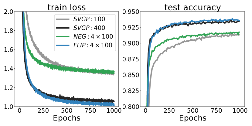
Figure 2: Flip-MNIST. We plot how left: train loss and right: test accuracy evolve with training. We observe the HVGP using FLIP: $4\times 100$ perform similarly with the SVGP using $400$ inducing points while the HVGP using NEG: $4\times 100$ perform substantially worse.

The additive GP reformulation in Eq. 18 ensures the independence between $\mathbf{u}_{0:T-1}$ in the prior, and we demonstrated the orthogonality of the decomposed RKHSs in Theorem 3.8. Thus it is tempting to modelling the variational posterior separately within each RKHS. Now we introduce the Harmonic Variational Gaussian Process (HVGPs), which enforces independence between $\mathbf{u}_{t}$ by letting $q(\mathbf{u}_{0:T-1})=\prod_{t=0}^{T-1}q_{t}(\mathbf{u}_{t})$. Then the variational posterior becomes

$$f =\sum_{t=0}^{T-1}f_{t},\;q_{t}(f_{t}(\cdot),\mathbf{u}_{t})=p_{t}(f_{t}(\cdot)|\mathbf{u}_{t})q_{t}(\mathbf{u}_{t}).$$ (21)

In other words, HVGPs use a variational posterior independently for each GP. We set $q_{t}(\mathbf{u}_{t})=\mathcal{N}(\bm{\mu}_{t},\mathbf{S}_{t})$ as Gaussians. In particular, if each $q_{t}$ uses $m$ inducing points, we term the model a $T\times m$ model. The variational posterior can be optimized by maximizing the ELBO,

where $q(\{f_{t}(\cdot)\}^{T-1}_{t=0}):=\prod_{t=0}^{T-1}\int p_{t}(f_{t}(\cdot)|\mathbf{u}_{t})q_{t}(\mathbf{u}_{t})d\mathbf{u}_{t}$.

How well does $\prod_{t=0}^{T-1}q_{t}(\mathbf{u}_{t})$ approximate the optimal Gaussian variational posterior $q^{\star}(\mathbf{u}_{0:T-1})$? $q^{\star}$ has a covariance $\mathbf{S}^{\star}\in\mathbb{R}^{Tm\times Tm}$, while HVGPs induce block diagonal structures. Fortunately, we can show that $\mathbf{S}^{\star}$ is approximately block diagonal if the input distribution is invariant to $G$.

Theorem 4.2.

If the input distribution $p$ is invariant to $G$, i.e., the random variable $\mathbf{x}\sim p$ and the random variable $G(\mathbf{x}),\mathbf{x}\sim p$ are identically distributed, then $\mathbf{S}^{\star}$ becomes block diagonal when the training size $N\to\infty$.

Theorem 4.2 indicates that the independent variational distributions $\prod_{t=0}^{T-1}q_{t}(\mathbf{u}_{t})$ in HVGPs accurately approximate $q^{\star}(\mathbf{u}_{0:T-1})$ when the input distribution is symmetric under the transformation $G$. The symmetry further makes it easy for $\{G^{t}(\mathbf{Z})\}_{t=0}^{T-1}$ to match the input distribution, which by Theorem 4.1 renders that the variational approximation in Eq. 20 with the optimal $q^{\star}(\mathbf{u}_{0:T-1})$ would be close to the true posterior.

We illustrate the gist with a flip-mnist problem, where each digit in the MNIST dataset is randomly flipped up-and-down or left-and-right. For a RBF kernel, we consider two variations of HVGPs in terms of the transformation: 1) Negation. We split input dimensions into two groups and negate them separately, resulting in a $4\times 100$ model. 2) Flipping the image up-and-down or left-and-right, resulting in a $4\times 100$ model. We compare them with SVGPs using $100,400$ inducing points, shown in Figure 2. This experiment highlights the importance of matching the transformation $G$ with the data distribution.

4.3 Computational Cost

Assume that we have a $J$-way transformation, and each way is $\tilde{T}_{j}$-cyclic. After decomposition this results in $\tilde{T}=\prod_{j=1}^{J}\tilde{T}_{j}$ complex-valued kernels and subsequently, $T=\prod_{j=1}^{J}(\lfloor\tilde{T}_{j}/2\rfloor+1)\geq\tilde{T}/2^{J}$ real-valued kernels. Let $T\times m$ represent using $m$ inducing points for each $t\in\{0,\dots,T-1\}$, and assume the mini-batch size $B=\mathcal{O}(m)$.

Time Complexity.

The computational cost boils down to the cost of computing $k_{t}(\mathbf{Z}_{t},\mathbf{Z}_{t})$ and the cost of variational inference. To compute $k_{t}(\mathbf{Z}_{t},\mathbf{Z}_{t})$, we need the kernel values $k(\mathbf{Z}_{t},G^{s}(\mathbf{Z}_{t}))$ for $s=0,...,\tilde{T}-1$. If we assume the cost of applying $G$ is $c_{G}$, then computing $\mathbf{K}_{\mathbf{u},\mathbf{u}}$ requires $\mathcal{O}(Tm\times\tilde{T}c_{G}+Tm^{2}\times\tilde{T})$ operations. Variational inference costs $\mathcal{O}(Tm^{3})$ time. Therefore, the overall complexity is $\mathcal{O}(Tm^{3}+2^{J}T^{2}m^{2}+2^{J}T^{2}mc_{G})$. We note $2^{J}\leq T$, and for a single-way transformation, the cost simplifies to $\mathcal{O}(Tm^{3}+T^{2}m^{2}+T^{2}mc_{G})$. In contrast, a SVGP with $Tm$ inducing points has the time complexity $\mathcal{O}(T^{3}m^{3})$. Furthermore, HVGPs support straightforward parallelisms by locating computations of $k_{t}$ on separate devices.

Space Complexity.

For computing $k_{t}(\mathbf{Z}_{t},\mathbf{Z}_{t})$, we need the kernel values $k(\mathbf{Z}_{t},G^{s}(\mathbf{Z}_{t}))$ for $s=0,\dots,\tilde{T}-1$, which implies the memory cost $\mathcal{O}(Tm^{2}\times\tilde{T})$. Adding the $\mathcal{O}(Tm^{2})$ memory for keeping variational approximations, the overall space complexity is, $\mathcal{O}(2^{J}T^{2}m^{2})$.

5 Related Works

The idea of applying Fourier analysis to kernels goes back at least to Bochner (1959). In machine learning, this led to a flowering of large-scale kernel methods based on random features (Rahimi & Recht, 2008; Yu et al., 2016; Dao et al., 2017). Bochner’s theorem also allows designing stationary kernels by modeling a spectral density (Wilson & Adams, 2013; Samo & Roberts, 2015; Parra & Tobar, 2017; Benton et al., 2019). On hyperspheres, zonal kernels are the counterpart of stationary kernels. Their spectral decomposition is given by spherical harmonics (Thomson & Tait, 1888; Morimoto, 1998). Although closely related, none of these works have considered the discrete Fourier transform adopted in our method.

HVGPs share many similarities with the works that propose decoupled (Cheng & Boots, 2017; Salimbeni et al., 2018) and orthogonal (Shi et al., 2020) inducing points. In particular, Shi et al. (2020) is also based on an orthogonal decomposition of the kernel and uses distinct groups of inducing points for them. However, their decomposition involves matrix inversion while ours can be computed using fast Fourier transforms.

Structured Kernel Interpolation (SKI) (Wilson & Nickisch, 2015; Wilson et al., 2015; Evans & Nair, 2018; Izmailov et al., 2018) places inducing points on a grid, leading to a structured $\mathbf{K}_{\mathbf{u}\mathbf{u}}$ that allows fast matrix-vector multiplications. For one-dimensional data, SKI exploits the Toeplitz structure of $\mathbf{K}_{\mathbf{u}\mathbf{u}}$ generated by stationary kernels. They first embed the Toeplitz matrix into a circulant matrix $\mathbf{C}$, and use the fact that circulant matrices can be diagonalized by the DFT (Tee, 2007) to enable fast computations:

$$\mathbf{C}=\mathbf{F}^{-1}\mathrm{diag}(\mathbf{F}\mathbf{c})\mathbf{F}.$$ (22)

Here $\mathbf{F}$ is the DFT matrix, and $\mathbf{c}$ is the first column of $\mathbf{C}$. This equation highlights a connection with our HKD: If we let $\mathbf{C}=[k(G^{t_{1}}(\mathbf{x}^{\prime}),G^{t_{2}}(\mathbf{x}))]_{t_{1},t_{2}=0}^{T-1}$, then $\mathbf{c}=[k(\mathbf{x},G^{0}(\mathbf{x}^{\prime})),...,k(\mathbf{x},G^{T-1}(\mathbf{x}^{\prime}))]$ is the sequence we constructed in Eq. 4, and the eigenvalues $\mathbf{F}\mathbf{c}$ recover our decomposition $[k_{t}(\mathbf{x},\mathbf{x}^{\prime})]_{t=0}^{T-1}$ by the discrete Fourier transform. In other words, our approach generalizes the structure of one-dimensional equally-spaced grids in SKI into arbitrary cyclic groups. Moreover, our method allows trainable inducing locations, which plays an important role in combating the curse of dimensionality.

Besides inducing points in the data space, a number of works have investigated inducing features in the frequency domain. However, these inducing features are either limited to specific kernels (Lázaro-Gredilla & Figueiras-Vidal, 2009; Hensman et al., 2017) or involve numerical approximations (Dutordoir et al., 2020; Burt et al., 2020). The implementation of Dutordoir et al. (2020) only supports data up to 8 dimensions.

Incorporating invariances with respect to input-space transformations into Gaussian processes is also investigated in a stream of works (Ginsbourger et al., 2016; Van der Wilk et al., 2019). Our work is orthogonal to them since we are not designing invariant models. Instead, we proposed a general inference method for GPs that can benefit from invariances in the data distribution. Relatedly, Solin & Särkkä (2020); Borovitskiy et al. (2020) studied Gaussian processes on Riemannian manifolds.

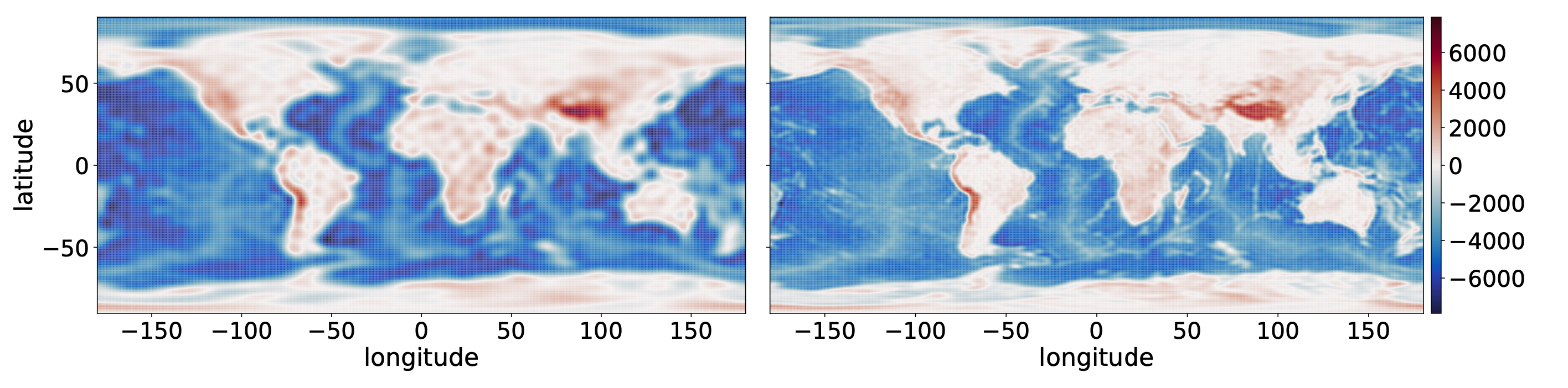
Figure 3: Predictive means of Earth elevations. We compare left: SVGP (M=1000) and right: HVGP ($13\times 1000$). The transformation in the HVGP moves each point eastwards by $15^{\text{o}}$ longitude. We observe that the HVGP ($13\times 1000$) fits the data more finely.

6 Experiments

We present empirical evaluations in this section. All results were obtained using NVIDIA Tesla P100 GPUs, except in Sec 6.3 we used NVIDIA Tesla T4. Code is available at https://github.com/ssydasheng/Harmonic-Kernel-Decomposition.

6.1 Earth Elevation

We adopt GPs to fit the ETOPO1 elevation data of the earth (Amante & Eakins, 2009). ETOPO1 bedrock models the Earth’s elevations from the bedrock surface underneath the ice sheets. A location is represented by the (longitude, latitude) pair, where longitude $\in[-180,180]$ and latitude $\in[-90,90]$. We build the dataset by choosing a location every $0.1$ degrees of longitude and latitude, resulting in $6,480,000$ data points. The dataset is randomly split for $72\%$ training, $8\%$ validating, and $20\%$ testing. We use a three dimensional RBF kernel between the Euclidean coordinates of any two (longitude, latitude) locations. Because moving two locations eastwards by the same amount of longitudes preserves their Euclidean distance, the kernel is invariant to the $T$-cyclic longitude translation:

$$G([\mathrm{lon},\mathrm{lat}]^{\top})=[\mathrm{lon}+\frac{360}{T},\mathrm{lat}]^{\top},$$ (23)

We set the period $T=12$ and $T=24$, so that $G$ moves a point eastwards by $30$ and $15$ degrees, respectively. Then we resolve Hermitian kernels to obtain $\lfloor 12/2\rfloor+1=7,\lfloor 24/2\rfloor+1=13$ real-valued kernels following Sec 3.4.

Model	Test RMSE	Test NLL	Time
SKI	0.145	1.313	1.18h
1k	0.252	0.040	0.38h
3k	0.208	-0.146	2.47h
5k	0.196	-0.203	8.70h
7x1k	0.189	-0.246	1.55h
13x1k	0.177	-0.314	4.25h

Table 1: Test performances on Earth elevations.

We compare SVGPs with $1k,3k,5k$ inducing points and the HVGPs with $7\times 1k,13\times 1k$ inducing points. We parallelize HVGPs using 4 GPUs, while SVGPs use only 1 GPU since it cannot be easily parallelized. All models are optimized using the Adam optimizer with learning rate 0.01 for 100K iterations. We also compare with SKI (Wilson & Nickisch, 2015). SKI runs into an out-of-memory error because of the large dataset, so we train it using a random $600,000$ subset of the training data. The performances are shown in Table 3 and the predictive means are visualized in Figure 3. From both the table and the figure, we observe using more inducing points in variational GP models fits the dataset substantially better. Moreover, because of the decomposed structures and the parallelisms, HVGPs use more inducing points but run faster. In comparison, SKI uses $1M$ inducing points and achieves the best RMSE, but its NLL is much worse compared to variational GPs.

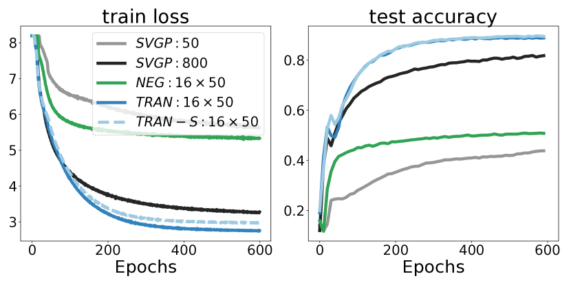
Figure 4: Translate-MNIST. We plot how left: train loss and right: test acc evolve with training. We compare $16\times M$ HVGPs with 1) NEG: negations; 2) TRAN: translations; 3) TRAN-S: translations with shared inducing points. We observe the HVGPs using translations even outperform the SVGP with $800$ inducing points while the HVGP using negations performs substantially worse. Moreover, though the HVGP with TRAN-S has only $50$ trainable inducing points, it performs similarly with the TRAN model.

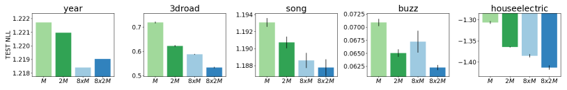
Figure 5: Test negative log-likelihoods on regression benchmarks. We compare using $M,2M,8\times M,8\times 2M$ for $M=1000$. We observe that the $8\times M,8\times 2M$ outperform the standard $M$ and $2M$ inducing points for the most datasets.

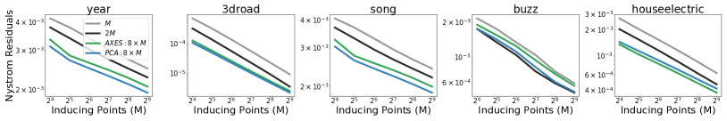
Figure 6: Nyström approximation errors measured by $\operatorname{\mathrm{trace}}(\mathbf{K}_{\mathbf{f}\mathbf{f}}-\mathbf{K}_{\mathbf{f}\mathbf{u}}\mathbf{K}_{\mathbf{u}\mathbf{u}}^{-1}\mathbf{K}_{\mathbf{u}\mathbf{f}})$. We compare SVGPs using $M,2M$ inducing points, and HVGPs with $8\times M$ inducing points. For the transformation in HVGPs, we include both the negation along the standard axes and along the principal components. We observe that negations along PCA directions usually outperform negations along standard axes, by demonstrating smaller approximation errors. And both variations of HVGPs perform better than the SVGPs. We also observe a consistency between the Nyström approximation errors and the regression performances. For example, the SVGP ($2M$) performs better than the HVGP ($8\times M$) for the buzz dataset in Figure 5, and this is similarly reflected by the Nyström approximation errors.

6.2 Translate-MNIST

The Elevation experiment uses one-way translations in HVGPs. In this section, we consider two-way translations for the Translate-MNIST dataset. The dataset is obtained by translating every MNIST image leftwards and downwards by random numbers of pixels. We use an RBF kernel with shared lengthscales. The HVGP uses a 2-way transformation $G$ by translating the image leftwards or downwards by $4$ pixels. Since the MNIST images are of size $28\times 28$, $G$ is $(7,7)$ cyclic. After resolving Hermitian kernels, we arrive at $(1+\lfloor 7/2\rfloor)\times(1+\lfloor 7/2\rfloor)=16$ groups.

We compare the $16\times 50$ translation HVGP with SVGPs using $50$ and $800$ inducing points. We further consider a variation of the HVGP by sharing the inducing points $\mathbf{Z}$ as in Theorem 4.1. We also include a $16\times 50$ HVGP with 4-way negations whose transformation does not match the input-space distribution. We optimize all models using the Adam optimizer with learning rate 0.001 for 100K iterations. The results are shown in Figure 4.

6.3 Regression Benchmarks

We also evaluate our method on standard regression benchmarks, whose training data sizes range from $200$ thousand to $1$ million. Following Wang et al. (2019), we use the Matérn 3/2 kernel with shared lengthscales. We consider the $J$-way composition of negations. Specifically, we conduct negations over PCA directions. We split the PCA directions into $J$ subsets, and applying negations over these subsets results in a $2^{J}\times m$ model. A visual comparison between the negation along axes and the negation along principal directions is shown in Figure 7.

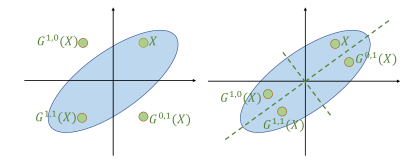
Figure 7: Negation along axes (left) and along principled directions (right). The shaded area represents the input distribution. We observe that $G^{1,0}(\mathbf{x}),G^{0,1}(\mathbf{x})$ are out of the data distribution when transforming along axes. In comparison, when transforming along PCA directions, the whole orbit is in-distribution.

We compare SVGPs using $M$ and $2M$ inducing points with HVGPs using $8\times M$ and $8\times 2M$ inducing points for $M=1000$. For HVGPs, we use $3$-way negations over PCA directions, and we use $8$ GPUs to place the computations of each GP in parallel. The results for negative log likelihoods (NLLs) are reported in Figure 5. We also report the root mean squared error (RMSE) performances in Figure 10 in the Appendix.

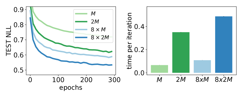
Figure 8: Test negative log-likelihoods during training and the training time per iteration for the 3droad dataset.

In Figure 8 we plot the evolution of the test negative log-likelihoods during training, and the training time per iteration, for the 3droad dataset. In Figure 8, we observe that using more inducing points enables learning the dataset more quickly and converging to a better minima. Furthermore, due to the benefit of parallelism, the $8\times M$ HVGP has comparable running time compared to the standard SVGP with $M$ inducing points. And it is much faster compared to the SVGP with $2M$ inducing points in spite of the improved performance. Moreover, the computational bottleneck of SVGPs lies in the Cholesky decomposition, which does not support easy parallelism.

The performance of variational GPs relies largely on how well can the inducing points summarize the dataset, which can be measured by the accuracy of Nyström approximation $\mathbf{K}_{\mathbf{f}\mathbf{f}}\approx\mathbf{K}_{\mathbf{f}\mathbf{u}}\mathbf{K}_{\mathbf{u}\mathbf{u}}^{-1}\mathbf{K}_{\mathbf{u}\mathbf{f}}$ (Drineas et al., 2005; Titsias, 2009; Burt et al., 2019). We compare the Nyström approximation errors with all methods, using the trace norm defined as $\operatorname{\mathrm{trace}}(\mathbf{K}_{\mathbf{f}\mathbf{f}}-\mathbf{K}_{\mathbf{f}\mathbf{u}}\mathbf{K}_{\mathbf{u}\mathbf{u}}^{-1}\mathbf{K}_{\mathbf{u}\mathbf{f}})$. For HVGPs, the trace norm is computed as

$$\sum_{t=0}^{T-1}\operatorname{\mathrm{trace}}(\mathbf{K}_{t,\mathbf{f}\mathbf{f}}-\mathbf{K}_{t,\mathbf{f}\mathbf{u}}\mathbf{K}_{t,\mathbf{u}\mathbf{u}}^{-1}\mathbf{K}_{t,\mathbf{u}\mathbf{f}}).$$ (24)

where we use $\mathbf{K}_{t,\cdot}$ to represent the kernel $k_{t}$. For each dataset, we randomly sample $3000$ points as $\mathbf{X}$ and use a Matérn 3/2 kernel whose lengthscales are set based on the median heuristic. We initialize the inducing points $\mathbf{Z}$ using K-means and optimize them to minimizing the trace error. We compare SVGPs, HVGPs with negations along axes, and HVGPs with negations along principled directions. The results are shown in Figure 6.

6.4 CIFAR-10 Classification

In this subsection we conduct experiments on the CIFAR10 classification problem using deep convolutional Gaussian processes (Blomqvist et al., 2019; Dutordoir et al., 2019), which combine the deep GP with the convolutional inducing features (Van der Wilk et al., 2017). Following the settings in Shi et al. (2020), we compare HVGP with SVGP on both one-layer and multi-layer convolutional GPs.

For HVGPs we use the negation transformations on the inducing filters $G(\mathbf{z})=-\mathbf{z}$. We compare HVGPs using 2xM, 4xM inducing points with SVGPs using M, 2M inducing points. For the HVGP (4xM), we use $4$ GPUs to achieve parallelism. We also compare with the 2-way decomposed model in Shi et al. (2020) termed as M+M. The results are summarized in Table 2. We observe that using more inducing filters results in better performances. In particular, the HVGP (4xM) achieves the best NLLs. Because of the parallelism, the HVGP (4xM) also has comparable running time with the HVGP (2xM), and both are faster than 2M and M+M for deep models.

M	Model	ACC	NLL	sec/iter
384x0, 1K	M	65.70$\pm$0.06	1.65$\pm$0.00	0.21
	2M	67.84$\pm$0.07	1.52$\pm$0.00	0.39
	M+M	67.67$\pm$ 0.07	1.50 $\pm$0.01	0.39
	2xM	66.26$\pm$1.11	1.76$\pm$0.17	0.45
	4xM	67.76$\pm$0.05	1.51$\pm$0.01	0.52
384x1, 1K	M	76.40$\pm$0.02	1.03$\pm$0.00	0.16
	2M	77.11$\pm$0.10	1.00$\pm$0.00	0.47
	M+M	77.48$\pm$0.10	0.98$\pm$0.01	0.41
	2xM	77.09$\pm$0.18	1.00$\pm$0.00	0.37
	4xM	77.30$\pm$0.17	0.95$\pm$0.00	0.36
384x2, 1K	M	79.01$\pm$0.11	0.86$\pm$0.00	0.17
	2M	80.27$\pm$0.04	0.81$\pm$0.00	0.52
	M+M	79.98 $\pm$0.21	0.80$\pm$0.01	0.46
	2xM	80.04$\pm$0.04	0.80$\pm$0.00	0.37
	4xM	80.52$\pm$0.20	0.75$\pm$0.01	0.37
384x3, 1K	M	82.41$\pm$0.08	0.73$\pm$0.01	0.40
	2M	-	-	-
	M+M	83.26$\pm$0.19	0.69$\pm$0.01	1.24
	2xM	84.97$\pm$0.08	0.60$\pm$0.00	0.90
	4xM	84.85$\pm$0.11	0.58$\pm$0.00	0.90

Table 2: Deep Convolutional GPs for CIFAR-10 classification. Previous SOTA (Shi et al., 2020) achieves ACC=$80.33$, NLL=0.82, and $1.25$ sec/iter. We use $384\text{x}\ell,1K$ to represent a $(\ell+1)$-layer model with a respective number of inducing points in each layer. We compare M, 2M, M+M, 2xM, 4xM. We used $4$ GPUs for the 4xM model to achieve parallelism. For the four-layer model, using 2M inducing points did not fit in memory. Instead we used a model with $(700\text{x}3,1600)$ inducing points and achieved ACC=$82.89\pm 0.05$, NLL=$0.73\pm 0.00$, and $1.10$ sec/iter.

7 Conclusion

We presented the harmonic kernel decomposition which exploited input-space symmetries to obtain an orthogonal kernel sum decomposition, based on which we introduced a scalable variational GP model and analyzed how well the model approximates the true posterior of the GP. We validated its superior performances in terms of scalability and accuracy through a range of empirical evaluations.

A Kernel Fourier Transform

We have shown that the Fourier series of length $T$ form the harmonic kernel decomposition with $T$ kernels. Intuitively, if $T\to\infty$, we obtain a “continuous” frequency representation of the kernel, which would be akin to a Fourier transform.

Consider the transformation $G^{\mathbf{s}}:\mathcal{X}\to\mathcal{X},\mathbf{s}\in\mathbb{R}^{J}$, corresponding to $J$-way transformations. We assume the transformation $G$ is $\mathbf{1}$-periodic: $G^{\mathbf{0}}(\mathbf{x})=G^{\mathbf{1}}(\mathbf{x})=\mathbf{x},G^{\mathbf{s}_{1}+\mathbf{s}_{2}}(\mathbf{x})=G^{\mathbf{s}_{1}}(G^{\mathbf{s}_{2}}(\mathbf{x})),\forall\mathbf{s}_{1},\mathbf{s}_{2}\in\mathbb{R}^{J}$. A kernel is $G$-invariant if for any $\mathbf{s}\in\mathbb{R}^{J}$, $k(G^{\mathbf{s}}(\mathbf{x}),G^{\mathbf{s}}(\mathbf{x}^{\prime}))=k(\mathbf{x},\mathbf{x}^{\prime})$.

Given the inputs $\mathbf{x},\mathbf{x}^{\prime}$, we consider the space of kernel values: $k(\mathbf{x},G^{\mathbf{s}}(\mathbf{x}^{\prime})),\mathbf{s}\in\mathbb{R}^{J}$. For $\mathbf{t}\in\mathbb{R}^{J}$, we define the complex-valued function $k_{\mathbf{t}}:\mathcal{X}\times\mathcal{X}\to\mathbb{C}$ using the Fourier transform,

$$k_{\mathbf{t}}(\mathbf{x},\mathbf{x}^{\prime})=\int_{\mathbb{R}^{J}}e^{-2\pi i\mathbf{s}^{\top}\mathbf{t}}k(\mathbf{x},G^{\mathbf{s}}(\mathbf{x}^{\prime}))\mathrm{d}\mathbf{s},$$ (25)

In this way, $k_{\mathbf{t}}(\mathbf{x},\mathbf{x}^{\prime})$ captures the frequency of $\mathbf{t}$ in the function $\mathbf{s}\to k(\mathbf{x},G^{\mathbf{s}}(\mathbf{x}^{\prime}))$. Similar to the harmonic kernel decomposition, we show an alternative representation of the kernel using $k_{t}$.

Theorem A.1 (Harmonic Kernel Representation).

$$k(\mathbf{x},\mathbf{x}^{\prime})=\int_{\mathbb{R}^{J}}k_{\mathbf{t}}(\mathbf{x},\mathbf{x}^{\prime})\mathrm{d}\mathbf{t}.$$ (26)

Moreover, $k_{\mathbf{t}}$ is a kernel for all $\mathbf{t}\in\mathbb{R}^{J}$.

Proof of Theorem A.1.

We prove this theorem by the following derivation,

$$\int_{\mathbb{R}^{J}}k_{\mathbf{t}}(\mathbf{x},\mathbf{x}^{\prime})\mathrm{d}\mathbf{t} =\int_{\mathbb{R}^{J}}\int_{\mathbb{R}^{J}}e^{-2\pi i\mathbf{s}^{\top}\mathbf{t}}k(\mathbf{x},G^{\mathbf{s}}(\mathbf{x}^{\prime}))\mathrm{d}\mathbf{s}\mathrm{d}\mathbf{t}=\int_{\mathbb{R}^{J}}k(\mathbf{x},G^{\mathbf{s}}(\mathbf{x}^{\prime}))\int_{\mathbb{R}^{J}}e^{-2\pi i\mathbf{s}^{\top}\mathbf{t}}\mathrm{d}\mathbf{t}\mathrm{d}\mathbf{s}$$

$$=\int_{\mathbb{R}^{J}}k(\mathbf{x},G^{\mathbf{s}}(\mathbf{x}^{\prime}))\delta_{\mathbf{s}}\mathrm{d}\mathbf{s}=k(\mathbf{x},\mathbf{x}^{\prime}).$$

where we used the property that the Fourier transform of the constant function is the delta function.

To show that $k_{t}$ is a kernel, we prove the following equality,

$$\int_{\mathbb{R}^{J}}\int_{\mathbb{R}^{J}}e^{-2\pi i\mathbf{t}^{\top}(\mathbf{s}_{2}-\mathbf{s}_{1})}k(G^{\mathbf{s}_{1}}(\mathbf{x}),G^{\mathbf{s}_{2}}(\mathbf{x}^{\prime}))\mathrm{d}\mathbf{s}_{1}\mathrm{d}\mathbf{s}_{2} =\int_{\mathbb{R}^{J}}\int_{\mathbb{R}^{J}}e^{-2\pi i\mathbf{t}^{\top}\mathbf{s}_{2}}k(\mathbf{x},G^{\mathbf{s}_{2}}(\mathbf{x}^{\prime}))\mathrm{d}\mathbf{s}_{1}\mathrm{d}\mathbf{s}_{2}$$

$$=\int_{\mathbb{R}^{J}}e^{-2\pi i\mathbf{t}^{\top}\mathbf{s}_{2}}k(\mathbf{x},G^{\mathbf{s}_{2}}(\mathbf{x}^{\prime}))\mathrm{d}\mathbf{s}_{2}=k_{\mathbf{t}}(\mathbf{x},\mathbf{x}^{\prime}).$$

∎

We demonstrate the Kernel Fourier Transform by considering a stationary kernel on the unit circle. We denote the input $x$ as the angle, then the kernel admits the form $k(x,x^{\prime})=\kappa(x-x^{\prime})$, where $\kappa$ is a periodic function of period $2\pi$. Let $\kappa_{0}(t)=\kappa(t)\mathbb{I}[0\leq t<2\pi]$, then

$$k(x,x^{\prime})=\kappa(x-x^{\prime})=\sum_{n\in\mathbb{Z}}\kappa_{0}(x-x^{\prime}-2\pi n),$$

Let $G^{s}(x)=x+2\pi s$, we obtain,

$$k_{t}(x,x^{\prime}) =\sum_{n\in\mathbb{Z}}\int_{\mathbb{R}}e^{-2\pi ist}\kappa_{0}(x-x^{\prime}-2\pi s-2\pi n)\mathrm{d}s=\frac{1}{2\pi}\sum_{n\in\mathbb{Z}}\int_{\mathbb{R}}e^{-i(x-x^{\prime}-2\pi n-w)t}\kappa_{0}(w)\mathrm{d}w$$

$$=e^{-it(x-x^{\prime})}\left[\frac{1}{2\pi}\int_{\mathbb{R}}e^{iwt}\kappa_{0}(w)\mathrm{d}w\right]\sum_{n\in\mathbb{Z}}e^{2\pi int}=e^{-it(x-x^{\prime})}\hat{\kappa}_{0}(t)\sum_{n\in\mathbb{Z}}\delta(t-n).$$

where $\hat{\kappa}_{0}$ is the inverse Fourier transform of $\kappa_{0}$. Then we have the Fourier series,

$$k(x,x^{\prime})=\int_{\mathbb{R}}k_{t}(x,x^{\prime})dt=\sum_{n\in\mathbb{Z}}\hat{\kappa}_{0}(n)e^{-in(x-x^{\prime})}.$$

B Inter-domain Inducing Points Formulation

We present an inter-domain inducing points interpretation of the harmonic kernel decomposition. An inter-domain inducing point is a function $w:\mathcal{X}\to\mathbb{C}$ whose inducing variable is defined as,

$$u_{w}=\int f(\mathbf{x})w(\mathbf{x})d\mathbf{x},$$ (27)

We introduce $T$ kinds of inter-domain inducing points. For $t=0,...,T-1$, given $\mathbf{z}_{t}\in\mathcal{X}$, the inter-domain inducing point of the $t$-th kind is,

$$w_{t} =\sum_{s=0}^{T-1}\mathbf{F}^{H}_{t,s}\delta_{G^{s}(\mathbf{z}_{t})},$$ (28)

$$u_{w_{t}} =\int f(\mathbf{x})w_{t}(\mathbf{x})d\mathbf{x}=\sum_{s=0}^{T-1}\mathbf{F}^{H}_{t,s}f(G^{s}(\mathbf{z}_{t})),$$ (29)

Therefore, we can generalize the kernel function to include inter-domain inputs,

$$k(\mathbf{x},w_{t}) =\mathbb{E}[f(\mathbf{x})u^{H}_{w_{t}}]=\sum_{s=0}^{T-1}\mathbf{F}_{t,s}k(\mathbf{x},G^{s}(\mathbf{z}_{t})),$$ (30)

$$k(w_{t},w^{\prime}_{t}) =\mathbb{E}[u_{w_{t}}u^{H}_{w^{\prime}_{t}}]=\sum_{s=0}^{T-1}\sum_{s^{\prime}=0}^{T-1}\mathbf{F}^{H}_{t,s}\mathbf{F}_{t,s^{\prime}}k(G^{s}(\mathbf{z}_{t}),G^{s^{\prime}}(\mathbf{z}^{\prime}_{t}))=\sum_{s=0}^{T-1}\mathbf{F}_{t,s}k(\mathbf{z}_{t},G^{s}(\mathbf{z}^{\prime}_{t})),$$ (31)

where the last equality is based on Lemma D.1. Furthermore, for $0\leq t\neq t^{\prime}\neq T-1$,

$$k(w_{t},w_{t^{\prime}}) =\sum_{s=0}^{T-1}\sum_{s^{\prime}=0}^{T-1}\mathbf{F}_{t,s}\mathbf{F}_{t^{\prime},s^{\prime}}^{H}k(G^{s}(\mathbf{z}_{t}),G^{s^{\prime}}(\mathbf{z}^{\prime}_{t^{\prime}}))=0.$$

where the last equality is based on Lemma D.2. We observe,

$$k(\mathbf{x},w_{t})=k_{t}(\mathbf{x},\mathbf{z}_{t});\;k(w_{t},w^{\prime}_{t})=k_{t}(\mathbf{z}_{t},\mathbf{z}^{\prime}_{t}).$$ (32)

Now we find that the proposed inter-domain inducing points formulation is equivalent to the kernel Fourier series. Furthermore, the equivalence also reinterprets HVGPs as standard SVGPs using inter-domain inducing points while enforcing block diagonal posterior covariances.

C More Experiments and Details

C.1 Toy Visualization

HVGPs are based on the decomposed GP formulation and assume independent variational posteriors. Therefore, the predictions on a target location $\mathbf{x}^{\star}$ can be decomposed as the combination of independent elements,

$$\mathcal{N}(\mathbf{0},\mathbf{K}_{\star\star}-\sum_{t=0}^{T-1}\mathbf{K}_{t,\star\mathbf{u}}\mathbf{K}_{t,\mathbf{u}\mathbf{u}}^{-1}\mathbf{K}_{t,\mathbf{u}\star}))+\sum_{t=0}^{T-1}\mathcal{N}(\mathbf{K}_{t,\star\mathbf{u}_{t}}\mathbf{K}_{t,\mathbf{u}_{t}\mathbf{u}_{t}}^{-1}\bm{\mu}_{t},\mathbf{K}_{t,\star\mathbf{u}_{t}}\mathbf{K}_{t,\mathbf{u}_{t}\mathbf{u}_{t}}^{-1}\mathbf{S}_{t}\mathbf{K}_{t,\mathbf{u}_{t}\mathbf{u}_{t}}^{-1}\mathbf{K}_{t,\star\mathbf{u}_{t}})$$

where we use $\mathbf{K}_{t,\cdot}$ to represent the kernel $k_{t}$. The first term in the prediction represents the error of the Nyström approximation, and the remaining terms contain the predictions from all subprocesses.

In this section we conduct a Snelson’s 1D toy experiment to visualize the posterior predictions and each term. We set $T=2,G(x)=-x,m=5$, which results in HVGP ($2\times 5$). Because the original training inputs are positive, we preprocess it by subtracting the inputs by the mean. The results are shown in Figure 9. We find that using $2\times 5$ inducing points fit the training data well, and generate reasonable predictive uncertainty as well. The predictions for the two GPs correspond to the symmetric and the antisymmetric fraction, respectively.

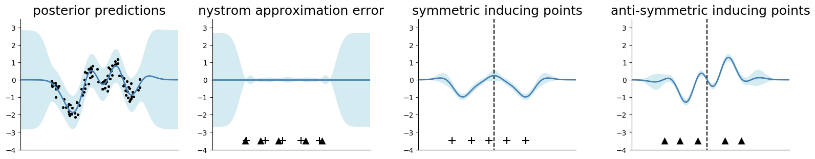
Figure 9: Posterior predictions on the Snelson dataset, where shaded bands correspond to intervals of $\pm 3$ standard deviation. The leftmost posterior prediction plot is the combination of the right three plots, plus the observation variance. We also visualize the associated inducing points for each plot. We observe that the HVGP predictions are separated as the symmetric fraction and the antisymmetric fraction.

C.2 Regression Benchmarks

We use the Matérn 3/2 kernel with shared lengthscales across input dimensions. For HVGPs, the transformation $G$ is by negating over PCA directions. We split the PCA directions into $J$ subsets, then apply negations over which results in a $2^{J}\times M$ model. We let the $j$-th subset contain the directions with the $j\text{th large},(J+j)\text{th large},...$ eigenvalues, so that the principal subspace is covered well. Except for the year dataset which has a standard train/test split, each dataset is randomly split into $64\%$ training, $16\%$ validating, $20\%$ testing sets and is averaged over $3$ random splits. We initialize the inducing points using K-means and initialize the kernel lengthscale using the median heuristic. The Gaussian likelihood variance is initialized at $0.1$. For all experiments, we optimize for 30k iterations with the Adam optimizer using learning rate 0.003 and batch size 256. We visualize the results for test RMSEs in Figure 10, and how each criterion evolves along training in Figure 11.

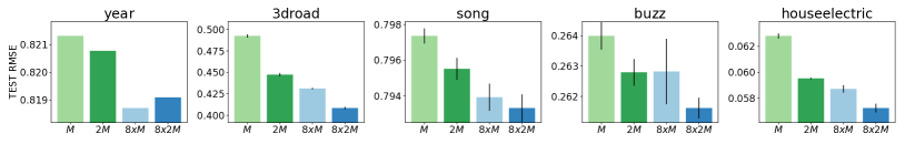
Figure 10: Test RMSEs on regression benchmarks. We compare SVGPs using $M,2M$ inducing points and HVGPs using $8\times M,8\times 2M$ inducing points, for $M=1000$.

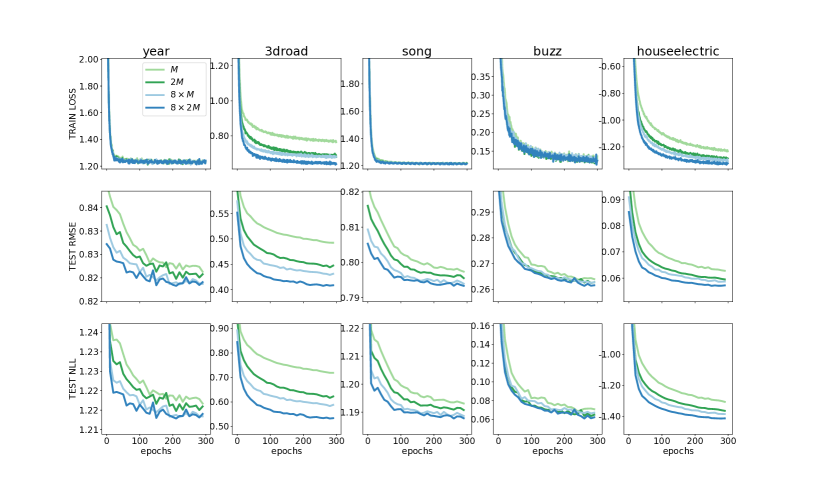
Figure 11: How train loss, test rmse, and test nll evolve during training. We compare SVGPs using $M,2M$ inducing points and HVGPs using $8\times M,8\times 2M$ inducing points, for $M=1000$.

C.3 CIFAR-10 Classification

Figure 12: Group Splitting for the HVGP ($4\times M$).

	1-layer	2-layer	3-layer	4-layer
filter size	5	5, 4	5,4,5	5,4,5,4
stride size	1	1,2	1,2,1	1,1,1,1
channel num	-	10	10,10	16,16,16
pooling	-	-	-	mean
pooling size	-	-	-	1,2,1
padding	SAME	SAME	SAME	SAME
M	384x0, 1K	384x1, 1K	384x2, 1K	384x3, 1K

Table 3: Model Configurations for Deep Convolutional Gaussian processes.

For deep Gaussian processes, we let $M_{l},h_{l}$ be the number of inducing points and the number of input units in the $l$-th layer, respectively. The variational posterior for the inducing points $\mathbf{U}^{l},\mathbf{U}^{l}\in\mathbb{R}^{M_{l}\times h_{l+1}}$ in the $l$-th layer is usually a multivariate Gaussian,

$$q(\mathrm{vec}(\mathbf{U}^{l}))=\mathcal{N}(\mathrm{vec}(\mathbf{M}^{l}),\bm{\Sigma}^{l}),$$ (33)

where $\mathbf{M}^{l}\in\mathbb{R}^{M_{l}\times h_{l+1}},\bm{\Sigma}^{l}\in\mathbb{R}^{(M_{l}h_{l+1})\times(M_{l}h_{l+1})}$ are the mean and the covariance, respectively. A commonly-used structure for $\bm{\Sigma}^{l}$ is the block-diagonal covariance (Salimbeni & Deisenroth, 2017) , i.e., assuming independence between output channels. However, the true posterior is not independent. Moreover, such covariance involves $h_{l+1}$ covariances of shape $M_{l}\times M_{l}$, which are both memory intensive and computation intensive. Therefore, following Park et al. (2018), we use the Kronecker-factored structure for the covariance, i.e., $\bm{\Sigma}^{l}=\bm{\Sigma}_{o}^{l}\otimes\bm{\Sigma}_{i}^{l}$, where $\bm{\Sigma}_{o}\in\mathbb{R}^{h_{l+1}\times h_{l+1}},\bm{\Sigma}_{i}\in\mathbb{R}^{M_{l}\times M_{l}}$ correspond to the output covariance and the input covariance, respectively.

Following Shi et al. (2020), all models were optimized using 270k iterations with the Adam optimizer using a learning rate 0.003 and a batch size 64. We anneal the learning rate by 0.25 every 50k iterations to ensure convergence. Unlike Shi et al. (2020) which used a zero mean function, we used a convolution mean function whose filter is 1 for the center pixel and 0 everywhere else, since we observe it with a better performance. We used the robust multi-class classification likelihood. For lower layers in the deep convolutional GP, we used multi-output GPs for each input patch (Blomqvist et al., 2019); for the output layer, we used the TICK kernel (Dutordoir et al., 2019). The patch kernels are RBF kernels with shared lengthscales, whose lengthscales and variances are initialized at $5$. The TICK location kernel is a Matérn 3/2 kernel whose lengthscales and variances are initialized at $1$ and $3$, respectively. To initialize the inducing filters, we use K-means samples from $\operatorname*{\mathrm{min}\vphantom{\mathrm{infsup}}}(100*M,10000)$ random input patches, while the inputs in all layers are obtained by forwarding the image through a random Xavier convnet.

For the HVGP ($2\times M$) we use the negation transformation on the inducing points $G(\mathbf{z})=-\mathbf{z}$. For the HVGP ($4\times M$), we also use the negation transformation over two groups that are determined by pixel locations, as shown in Figure 12.

D Proofs

D.1 Lemmas

Lemma D.1.

For any $t=0,...,T-1$, $\mathbf{x},\mathbf{x}^{\prime}\in\mathcal{X}$,

$$\sum_{s=0}^{T-1}\sum_{s^{\prime}=0}^{T-1}\mathbf{F}^{H}_{t,s}\mathbf{F}_{t,s^{\prime}}k(G^{s}(\mathbf{x}),G^{s^{\prime}}(\mathbf{x}^{\prime}))=\sum_{s=0}^{T-1}\mathbf{F}_{t,s}k(\mathbf{x},G^{s}(\mathbf{x}^{\prime})).$$

Proof.

We prove the equality by the expression of $\mathbf{F}$,

$$\frac{1}{T^{2}}\sum_{s=0}^{T-1}\sum_{s^{\prime}=0}^{T-1}e^{-i\frac{2\pi t}{T}(s^{\prime}-s)}k(G^{s}(\mathbf{x}),G^{s+(s^{\prime}-s)}(\mathbf{x}^{\prime}))=\frac{1}{T}\sum_{s_{0}=0}^{T-1}e^{-i\frac{2\pi t}{T}s_{0}}k(\mathbf{x},G^{s_{0}}(\mathbf{x}^{\prime})),$$

where we used the kernel invariance to $G$. Also, since $G$ is $T$-cyclic, we changed the variable $s^{\prime}-s$ to $s_{0}$ and $s_{0}$ still ranges from $0$ to $T-1$. ∎

Lemma D.2.

For any $0\leq t_{1}\neq t_{2}\leq T-1$, $\mathbf{x},\mathbf{x}^{\prime}\in\mathcal{X}$,

$$\sum_{s_{1}=0}^{T-1}\sum_{s_{2}=0}^{T-1}\mathbf{F}^{H}_{t_{1},s_{1}}\mathbf{F}_{t_{2},s_{2}}k(G^{s_{1}}(\mathbf{x}),G^{s_{2}}(\mathbf{x}^{\prime}))=0,$$ (34)

$$\sum_{s_{1}=0}^{T-1}\sum_{s_{2}=0}^{T-1}\mathbf{F}_{t_{1},s_{1}}\mathbf{F}^{H}_{t_{2},s_{2}}k(G^{s_{1}}(\mathbf{x}),G^{s_{2}}(\mathbf{x}^{\prime}))=0,$$ (35)

Proof.

Below we prove 34. The proof of 35 follows similarly.

$$\sum_{s_{1}=0}^{T-1}\sum_{s_{2}=0}^{T-1}\mathbf{F}^{H}_{t_{1},s_{1}}\mathbf{F}_{t_{2},s_{2}}k(G^{s_{1}}(\mathbf{x}),G^{s_{2}}(\mathbf{x}^{\prime}))=\sum_{s_{1}=0}^{T-1}\sum_{s_{2}=0}^{T-1}\mathbf{F}^{H}_{t_{1},s_{1}}\mathbf{F}_{t_{2},s_{1}+s_{2}}k(G^{s_{1}}(\mathbf{x}),G^{s_{1}+s_{2}}(\mathbf{x}^{\prime}))$$

$$=\sum_{s_{2}=0}^{T-1}k(\mathbf{x},G^{s_{2}}(\mathbf{x}^{\prime}))\sum_{s_{1}=0}^{T-1}\mathbf{F}^{H}_{t_{1},s_{1}}\mathbf{F}_{t_{2},s_{1}+s_{2}}=\sum_{s_{2}=0}^{T-1}k(\mathbf{x},G^{s_{2}}(\mathbf{x}^{\prime}))e^{-i\frac{2\pi ts_{2}}{T}}\sum_{s_{1}=0}^{T-1}\mathbf{F}^{H}_{t_{1},s_{1}}\mathbf{F}_{t_{2},s_{1}}=0.$$

In the last step, $\sum_{s_{1}=0}^{T-1}\mathbf{F}^{H}_{t_{1},s_{1}}\mathbf{F}_{t_{2},s_{1}}=0$ whenever $t_{1}\neq t_{2}$. This is because the columns of $\mathbf{F}$ form an orthogonal basis over the set of $T$-dimensional complex vectors. ∎

Lemma D.3.

Under the harmonic formulation, for $\mathbf{x}\in\mathcal{X}$,

$$f_{t}(\mathbf{x})=\sum_{s=0}^{T-1}\mathbf{F}^{H}_{t,s}f(G^{s}(\mathbf{x})).$$ (36)

Proof.

We consider a marginal distribution on a subset of function values,

$$p(\{f(G^{s}(\mathbf{x}))\}_{s=0}^{T-1},\{f_{0}(G^{s}(\mathbf{x}))\}_{s=0}^{T-1},...,\{f_{T-1}(G^{s}(\mathbf{x}))\}_{s=0}^{T-1}),$$

The distribution can be represented as,

$$f(G^{s}(\mathbf{x})) =\sum_{t=0}^{T-1}f_{t}(G^{s}(\mathbf{x})),s=0,...,T-1,$$

$$\mathbf{f}_{t}(G^{0:T-1}(\mathbf{x})) \sim\mathcal{N}(0,\mathbf{K}_{t}(G^{0:T-1}(\mathbf{x}),G^{0:T-1}(\mathbf{x}))),$$

We first investigate the structure of the kernel matrix $\mathbf{K}_{t}$,

$$k_{t}(G^{j}(\mathbf{x}),G^{j^{\prime}}(\mathbf{x})) =\sum_{s=0}^{T-1}\mathbf{F}_{t,s}k(G^{j}(\mathbf{x}),G^{s+j^{\prime}}(\mathbf{x}))=\sum_{s=0}^{T-1}\mathbf{F}_{t,s}k(\mathbf{x},G^{s+j^{\prime}-j}(\mathbf{x}))=\sum_{s=0}^{T-1}\mathbf{F}_{t,s+j-j^{\prime}}k(\mathbf{x},G^{s}(\mathbf{x}))$$

$$=e^{-\frac{2\pi it(j-j^{\prime})}{T}}\sum_{s=0}^{T-1}\mathbf{F}_{t,s}k(\mathbf{x},G^{s}(\mathbf{x}))=e^{-\frac{2\pi it(j-j^{\prime})}{T}}k_{t}(\mathbf{x},\mathbf{x}),$$

Therefore, the matrix $\mathbf{K}_{t}=[k_{t}(\mathbf{x},\mathbf{x})e^{-\frac{2\pi it(j-j^{\prime})}{T}}]_{j,j^{\prime}=0}^{T-1}$. Let $\epsilon_{t}\in\mathbb{R}$ be a random Gaussian noise, then the random vector of $f_{t}$ can be written as,

$$\mathbf{f}_{t}(G^{0:T-1}(\mathbf{x}))=[\sqrt{k_{t}(\mathbf{x},\mathbf{x})}e^{-\frac{2\pi itj}{T}}\epsilon_{t}]_{j=0}^{T-1},$$ (37)

Now we can compute the RHS in the lemma,

$$\sum_{s=0}^{T-1}\mathbf{F}^{H}_{t,s}f(G^{s}(\mathbf{x})) =\sum_{s=0}^{T-1}\mathbf{F}^{H}_{t,s}\sum_{t^{\prime}=0}^{T-1}f_{t^{\prime}}(G^{s}(\mathbf{x}))=\sum_{t^{\prime}=0}^{T-1}\sum_{s=0}^{T-1}\mathbf{F}^{H}_{t,s}f_{t^{\prime}}(G^{s}(\mathbf{x})),$$

If $t^{\prime}=t$,

$$\sum_{s=0}^{T-1}\mathbf{F}^{H}_{t,s}f_{t}(G^{s}(\mathbf{x})) =\sum_{s=0}^{T-1}\mathbf{F}^{H}_{t,s}\sqrt{k_{t}(\mathbf{x},\mathbf{x})}e^{-\frac{2\pi its}{T}}\epsilon_{t}=\sqrt{k_{t}(\mathbf{x},\mathbf{x})}\epsilon_{t}=f_{t}(\mathbf{x}).$$ (38)

If $t^{\prime}\neq t$,

$$\sum_{s=0}^{T-1}\mathbf{F}^{H}_{t,s}f_{t^{\prime}}(G^{s}(\mathbf{x})) =\sum_{s=0}^{T-1}\mathbf{F}^{H}_{t,s}\sqrt{k_{t^{\prime}}(\mathbf{x},\mathbf{x})}e^{-\frac{2\pi it^{\prime}s}{T}}\epsilon_{t}=\sqrt{k_{t^{\prime}}(\mathbf{x},\mathbf{x})}\epsilon_{t}\sum_{s=0}^{T-1}e^{\frac{2\pi i(t-t^{\prime})}{T}}=0.$$ (39)

Therefore,

$$\sum_{s=0}^{T-1}\mathbf{F}^{H}_{t,s}f(G^{s}(\mathbf{x}))=f_{t}(\mathbf{x}).$$ (40)

Because this holds for all marginal distributions, it holds as well for the function samples from Gaussian processes.∎

D.2 Proofs for Sec 3

Proof of Proposition 3.3.

The equality can be directly proven,

$$k_{t}(\mathbf{x},G(\mathbf{x}^{\prime})) =\sum_{s=0}^{T-1}\mathbf{F}_{t,s}k(\mathbf{x},G^{s+1}(\mathbf{x}^{\prime}))=\sum_{s=0}^{T-1}\mathbf{F}_{t,s-1}k(\mathbf{x},G^{s}(\mathbf{x}^{\prime}))$$

$$=\sum_{s=0}^{T-1}\frac{1}{T}e^{-i\frac{2\pi t(s-1)}{T}}k(\mathbf{x},G^{s}(\mathbf{x}^{\prime}))=e^{i\frac{2\pi t}{T}}k_{t}(\mathbf{x},\mathbf{x}^{\prime}).$$ (41)

∎

Proof of Theorem 3.5.

The equality can be directly proven,

$$\sum_{t=0}^{T-1}k_{t}(\mathbf{x},\mathbf{x}^{\prime}) =\sum_{t=0}^{T-1}\sum_{s=0}^{T-1}\frac{1}{T}e^{-i\frac{2\pi st}{T}}k(\mathbf{x},G^{s}(\mathbf{x}^{\prime}))=\frac{1}{T}\sum_{s=0}^{T-1}k(\mathbf{x},G^{s}(\mathbf{x}^{\prime}))\sum_{t=0}^{T-1}e^{-i\frac{2\pi st}{T}}=\frac{1}{T}\sum_{s=0}^{T-1}k(\mathbf{x},G^{s}(\mathbf{x}^{\prime}))T\delta_{s}=k(\mathbf{x},\mathbf{x}^{\prime}).$$

To prove that $k_{t}$ is a kernel, we observe from Lemma D.1 that $k_{t}(\mathbf{x},\mathbf{x}^{\prime})=\mathbf{F}_{t,:}^{H}\mathbf{K}\mathbf{F}_{t,:}$, where $\mathbf{K}=[k(G^{s_{1}}(\mathbf{x}),G^{s_{2}}(\mathbf{x}^{\prime}))]_{s_{1},s_{2}=0}^{T-1}$. Since $k$ is a kernel, we conclude that $k_{t}(\mathbf{x},\mathbf{x}^{\prime})=\mathbf{F}_{t,:}^{H}\mathbf{K}\mathbf{F}_{t,:}$ is a kernel as well.

∎

Proof of Lemma 3.6.

We firstly prove that, for all $t_{1}\neq t_{2}$ and $\mathbf{x},\mathbf{x}^{\prime}$, $\langle k_{t_{1}}(\cdot,\mathbf{x}),k_{t_{2}}(\cdot,\mathbf{x}^{\prime})\rangle_{\mathcal{H}_{k}}=0$. The RKHS inner product can be computed as,

$$\langle k_{t_{1}}(\cdot,\mathbf{x}),k_{t_{2}}(\cdot,\mathbf{x}^{\prime})\rangle_{\mathcal{H}_{k}}=\sum_{s_{1}=0}^{T-1}\sum_{s_{2}=0}^{T-1}\mathbf{F}_{t_{1},s_{1}}\mathbf{F}^{H}_{t_{2},s_{2}}k(G^{s_{1}}(\mathbf{x}),G^{s_{2}}(\mathbf{x}^{\prime}))=0,$$ (42)

where the last equality is due to Lemma D.2.

Moreover, if the functions $f,g$ can be written as linear combinations of the corresponding kernels,

$$f(\mathbf{x})=\sum_{s}a_{s}k_{t_{1}}(\mathbf{x},\mathbf{x}^{s}_{t_{1}});\;g(\mathbf{x})=\sum_{s}b_{s}k_{t_{2}}(\mathbf{x},\mathbf{x}^{s}_{t_{2}})$$

Following that $\langle k_{t_{1}}(\cdot,\mathbf{x}),k_{t_{2}}(\cdot,\mathbf{x}^{\prime})\rangle_{\mathcal{H}_{k}}$ for all $\mathbf{x},\mathbf{x}^{\prime}$, $\langle f,g\rangle_{\mathcal{H}_{k}}=0$ as well.

Based on Moore-Aronszajn Theorem (Aronszajn, 1950; Berlinet & Thomas-Agnan, 2011), the RKHS spaces $\mathcal{H}_{k_{t_{1}}}$ and $\mathcal{H}_{k_{t_{1}}}$ are the set of functions which are pointwise limits of Cauchy sequences in the form $f_{n}(\mathbf{x})=\sum_{s}a_{s}k_{t_{1}}(\mathbf{x},\mathbf{x}^{s}_{t_{1}})$ and $g_{n}(\mathbf{x})=\sum_{s}b_{s}k_{t_{2}}(\mathbf{x},\mathbf{x}^{s}_{t_{2}})$, respectively. Moreover, based on the Berlinet & Thomas-Agnan (2011, Lemma 5), the inner product of two pointwisely convergent Cauchy sequences also converges. We conclude that for any $f\in\mathcal{H}_{k_{t_{1}}},g\in\mathcal{H}_{k_{t_{2}}}$, $\langle f,g\rangle_{\mathcal{H}_{k}}=0$. ∎

Proof of Proposition 3.7.

Without loss of generality, we only need to prove that,

$$\mathcal{H}_{1}\cap\mathcal{H}_{2}=\{0\},$$

Firstly, $0\in\mathcal{H}_{1},0\in\mathcal{H}_{2}$ because $\mathcal{H}_{1}$ and $\mathcal{H}_{2}$ are Hilbert spaces. Then we assume another function $f\neq 0$ and $f\in\mathcal{H}_{1}\cap\mathcal{H}_{2}$. By Lemma 3.6, $\|f\|_{\mathcal{H}_{k}}=\langle f,f\rangle_{\mathcal{H}_{k}}=0$, which is contradictory to $f\neq 0$ and $\mathcal{H}_{k}$ being a Hilbert space. ∎

Proof of Theorem 3.8.

We use $\mathcal{H}_{t}$ to represent the RKHS corresponding to the kernel $k_{t}$. Given a function $f\in\mathcal{H}_{k}$, we firstly assume $f$ can be written as a linear combination of the kernel functions,

$$f(\mathbf{x})=\sum_{s}a_{s}k(\mathbf{x},\mathbf{x}^{s}),$$

Based on the kernel sum decomposition, we can rewrite $f$,

$$f(\mathbf{x})=\sum_{s}a_{s}\sum_{t=0}^{T-1}k_{t}(\mathbf{x},\mathbf{x}^{s})=\sum_{t=0}^{T-1}\underbrace{\sum_{s}a_{s}k_{t}(\mathbf{x},\mathbf{x}^{s})}_{:=f_{t}(\mathbf{x})},$$

Because $f_{t}$ is a linear combination of $k_{t}$, $f_{t}\in\mathcal{H}_{t}$, for $t=0,...,T-1$. Proposition 3.7 states that the RKHSs $\mathcal{H}_{t_{1}},\mathcal{H}_{t_{2}}$ are disjoint except the zero function, thus $f=\sum_{t=0}^{T-1}f_{t}$ is a unique expansion of $f$ to these RKHSs. Moreover, we can represent the function $f$ alternatively,

$$f(\mathbf{x}) =\langle f,k(\mathbf{x},\cdot)\rangle_{\mathcal{H}_{k}}=\sum_{t=0}^{T-1}\langle f,k_{t}(\mathbf{x},\cdot)\rangle_{\mathcal{H}_{k}}=\sum_{t=0}^{T-1}\langle\sum_{t^{\prime}=0}^{T-1}f_{t^{\prime}},k_{t}(\mathbf{x},\cdot)\rangle_{\mathcal{H}_{k}}=\sum_{t=0}^{T-1}\langle f_{t},k_{t}(\mathbf{x},\cdot)\rangle_{\mathcal{H}_{k}},$$

where the last equality uses the orthogonality between RKHSs. By using the orthogonality again, we also show that,

$$\langle f_{t},k_{t}(\mathbf{x},\cdot)\rangle_{\mathcal{H}_{k}} =\langle f_{t},\sum_{t^{\prime}=0}^{T_{1}}k_{t^{\prime}}(\mathbf{x},\cdot)\rangle_{\mathcal{H}_{k}}=\langle f_{t},k(\mathbf{x},\cdot)\rangle_{\mathcal{H}_{k}}=f_{t}(\mathbf{x}),$$ (43)

Therefore, $f(\mathbf{x})=\sum_{t=0}^{T-1}\langle f,k_{t}(\mathbf{x},\cdot)\rangle_{\mathcal{H}_{k}}$ uniquely separates $f$ into these RKHSs. More generally, if $f$ is the pointwise limits of Cauchy sequences of functions in the form of linear combinations of the kernel function. Based on the Berlinet & Thomas-Agnan (2011, Lemma 5), the inner product of two pointwisely convergent Cauchy sequences also converges. We conclude that for any $f\in\mathcal{H}_{k}$,

$$f(\mathbf{x})=\sum_{t=0}^{T-1}\langle f,k_{t}(\mathbf{x},\cdot)\rangle_{\mathcal{H}_{k}},$$ (44)

uniquely decomposes the function $f$ into the RKHSs $\mathcal{H}_{t},t=0,...,T-1$.

Based on Berlinet & Thomas-Agnan (2011, Theorem 5), the squared RKHS norm of $f$ can be written as the sum of squared RKHS norms,

$$\|f\|_{\mathcal{H}_{k}}^{2}=\sum_{t=0}^{T-1}\|f_{t}\|_{\mathcal{H}_{t}}^{2}.$$

∎

D.3 Proof of Sec 4

Proof of Theorem 4.1.

Under the HVGP formulation, the inducing variable $u_{t}=f_{t}(\mathbf{z})$. From Lemma D.3, we have $f_{t}(\mathbf{z})=\sum_{s=0}^{T-1}\mathbf{F}^{H}_{t,s}f(G^{s}(\mathbf{z}))$.

Under the inter-domain formulation, let $w_{t}$ be the inter-domain inducing point corresponding to $\mathbf{z}$ in $k_{t}$,

$$w_{t}=\sum_{s=0}^{T-1}\mathbf{F}^{H}_{t,s}\delta_{G^{s}(\mathbf{z})},$$

Then the inducing variable corresponding to $w_{t}$ is,

$$u_{w_{t}}=\int f(\mathbf{x})w_{t}(\mathbf{x})d\mathbf{x}=\sum_{s=0}^{T-1}\mathbf{F}^{H}_{t,s}f(G^{s}(\mathbf{z})),$$ (45)

Therefore, the two inducing variables are the same,

$$u_{w_{t}}=u_{t}.$$ (46)

Therefore, the variational posterior under the harmonic formulation can be rewritten in an inter-domain SVGP form,

$$q^{inter}(f,\mathbf{U})=p(f|\mathbf{U};\{\mathbf{w}_{t}\}_{t=0}^{T-1})q(\mathrm{vec}(\mathbf{U})),$$ (47)

where $\mathbf{U}:=[\mathbf{u}_{0},...,\mathbf{u}_{T-1}]^{\top}$ and $p$ is the inter-domain Gaussian process.

Now we connect the inter-domain SVGP to the standard SVGP using $\{G^{t}(\mathbf{Z})\}_{t=0}^{T-1}$. For the standard SVGP, the inducing variables are $\mathbf{v}_{t}=f(G^{t}(\mathbf{Z}))$, and $\mathbf{V}:=[\mathbf{v}_{0},...,\mathbf{v}_{T-1}]^{\top}\in\mathbb{C}^{T\times m}$. For the inter-domain SVGP, the inducing variables are $\mathbf{u}_{t}$. As shown in Eq. 45, $\mathbf{u}_{t}=\sum_{s=0}^{T-1}\mathbf{F}^{H}_{t,s}\mathbf{v}_{s}$, then we have the equality,

$$\mathbf{U}=\mathbf{F}^{H}\mathbf{V},$$ (48)

Because of the bijective linearity,

$$p(f|\mathbf{U};\{\mathbf{w}_{t}\}_{t=0}^{T-1})=p(f|\mathbf{V};\{G^{t}(\mathbf{Z})\}_{t=0}^{T-1}),$$ (49)

Furthermore, the variational posterior for $\mathbf{V}$ is $\mathcal{N}(\mathrm{vec}(\mathbf{V})|\mathrm{vec}(\mathbf{M}_{v}),\mathbf{S}_{v})$, which is equivalent to the variational posterior for $\mathbf{U}$,

$$q(\mathrm{vec}(\mathbf{U}))=\mathcal{N}(\mathrm{vec}(\mathbf{U})|\mathrm{vec}(\mathbf{F}^{H}\mathbf{M}_{v}),(\mathbf{I}\otimes\mathbf{F}^{H})\mathbf{S}_{v}(\mathbf{I}\otimes\mathbf{F})).$$

So the argument has been proved.

∎

Lemma D.4 (Variational Gaussian Approximations).

Let $\mathcal{N}(\bm{\mu},\mathbf{S})$ be a Gaussian variational posterior for a SVGP, then the optimal $\mathbf{S}^{\star}$ is in the form of,

$$\mathbf{S}^{\star}=\mathbf{K}_{\mathbf{u}\mathbf{u}}\left(\mathbf{K}_{\mathbf{u}\mathbf{u}}+\mathbf{K}_{\mathbf{u}\mathbf{f}}\bm{\Lambda}\mathbf{K}_{\mathbf{f}\mathbf{u}}\right)^{-1}\mathbf{K}_{\mathbf{u}\mathbf{u}}.$$ (50)

where $\bm{\Lambda}=\mathrm{diag}([\lambda_{n}]_{n=1}^{N})$ is diagonal,

$$\lambda_{n}=-2\nabla_{\sigma^{2}_{n}}\mathbb{E}_{q(f_{n})}[\log p(y_{n}|f_{n})],$$ (51)

where $\sigma^{2}_{n}$ is the predictive variance of $f_{n}$ under the variational posterior.

Proof.

Given the variational posterior, the predictive distribution of $f_{n}$ can be computed as,

$$\mathcal{N}(\mathbf{k}_{f\mathbf{u}}\mathbf{K}_{\mathbf{u}\mathbf{u}}^{-1}\bm{\mu},k_{ff}+\mathbf{k}_{f\mathbf{u}}\mathbf{K}_{\mathbf{u}\mathbf{u}}^{-1}(\mathbf{S}-\mathbf{K}_{\mathbf{u}\mathbf{u}})\mathbf{K}_{\mathbf{u}\mathbf{u}}^{-1}\mathbf{k}_{\mathbf{u}f}),$$

where we denote the predictive variance as $\sigma_{n}^{2}$. The variational posterior is optimized by maximizing the ELBO, which can be computed as,

$$\mathcal{L}=\sum_{n=1}^{N}\mathbb{E}_{q(f_{n})}[\log p(y_{n}|f_{n})]-\mathrm{KL}\left(\mathcal{N}(\bm{\mu},\mathbf{S})||\mathcal{N}(\mathbf{0},\mathbf{K}_{\mathbf{u}\mathbf{u}})\right),$$

We compute the derivatives of $\mathcal{L}$ towards $\mathbf{S}$,

$$\nabla_{\mathbf{S}}\mathcal{L} =-\frac{1}{2}\sum_{n=1}^{N}\lambda_{n}\nabla_{\mathbf{S}}\sigma_{n}^{2}-\frac{1}{2}(\mathbf{K}_{\mathbf{u}\mathbf{u}}^{-1}-\mathbf{S}^{-1})=-\frac{1}{2}\mathbf{K}_{\mathbf{u}\mathbf{u}}^{-1}(\sum_{n=1}^{N}\lambda_{n}\mathbf{k}_{\mathbf{u}f_{n}}\mathbf{k}_{f_{n}\mathbf{u}})\mathbf{K}_{\mathbf{u}\mathbf{u}}^{-1}-\frac{1}{2}(\mathbf{K}_{\mathbf{u}\mathbf{u}}^{-1}-\mathbf{S}^{-1})$$

$$=-\frac{1}{2}\mathbf{K}_{\mathbf{u}\mathbf{u}}^{-1}\mathbf{K}_{\mathbf{u}\mathbf{f}}\bm{\Lambda}\mathbf{K}_{\mathbf{f}\mathbf{u}}\mathbf{K}_{\mathbf{u}\mathbf{u}}^{-1}-\frac{1}{2}\mathbf{K}_{\mathbf{u}\mathbf{u}}^{-1}+\frac{1}{2}\mathbf{S}^{-1},$$ (52)

Let the derivative be zero, we obtain the optimal $\mathbf{S}^{\star}$,

$$\mathbf{S}^{\star}=\mathbf{K}_{\mathbf{u}\mathbf{u}}(\mathbf{K}_{\mathbf{u}\mathbf{u}}+\mathbf{K}_{\mathbf{u}\mathbf{f}}\bm{\Lambda}\mathbf{K}_{\mathbf{f}\mathbf{u}})^{-1}\mathbf{K}_{\mathbf{u}\mathbf{u}}.$$

∎

Proof of Theorem 4.2.

Based on Lemma D.4, the optimal posterior covariance is

$$\mathbf{S}^{\star}=\mathbf{K}_{\mathbf{u}\mathbf{u}}\left(\mathbf{K}_{\mathbf{u}\mathbf{u}}+\mathbf{K}_{\mathbf{u}\mathbf{f}}\bm{\Lambda}\mathbf{K}_{\mathbf{f}\mathbf{u}}\right)^{-1}\mathbf{K}_{\mathbf{u}\mathbf{u}},$$ (53)

Given that $\mathbf{K}_{\mathbf{u}\mathbf{u}}$ is block diagonal, by the continuous mapping theorem, it remains to prove that $\mathbf{K}_{\mathbf{u}\mathbf{f}}\bm{\Lambda}\mathbf{K}_{\mathbf{f}\mathbf{u}}$ approaches block diagonal.

Firstly we assume that Hermitian kernels are not resolved, thus $\mathbf{K}_{\mathbf{f}\mathbf{u}}=\mathbf{K}_{\mathbf{u}\mathbf{f}}^{H}$. Because $\lambda_{n}$ only depends on $(\mathbf{x}_{n},y_{n})$, for the $(\mathbf{z}_{t},\mathbf{z}_{t^{\prime}})$ off-diagonal element in $\mathbf{K}_{\mathbf{u}\mathbf{f}}\bm{\Lambda}\mathbf{K}_{\mathbf{f}\mathbf{u}}$,

$$\frac{1}{N}\sum_{n=1}^{N}\lambda_{n}k_{t}(\mathbf{z}_{t},\mathbf{x}_{n})k_{t^{\prime}}^{H}(\mathbf{z}_{t^{\prime}},\mathbf{x}_{n})\to\mathbb{E}_{p(\mathbf{x})p(y|\mathbf{x})}[\lambda(\mathbf{x},y)k_{t}(\mathbf{z}_{t},\mathbf{x})k^{H}_{t^{\prime}}(\mathbf{z}_{t^{\prime}},\mathbf{x})]=\mathbb{E}_{p(\mathbf{x})}[\mathbb{E}_{p(y|\mathbf{x})}[\lambda(\mathbf{x},y)]k_{t}(\mathbf{z}_{t},\mathbf{x})k^{H}_{t^{\prime}}(\mathbf{z}_{t^{\prime}},\mathbf{x})],$$

We let $\hat{\lambda}(\mathbf{x}):=\mathbb{E}_{p(y|\mathbf{x})}[\lambda(\mathbf{x},y)]$, then the formula can be further computed as,

$$\mathbb{E}_{p(\mathbf{x})}[\hat{\lambda}(\mathbf{x})k_{t}(\mathbf{z}_{t},\mathbf{x})k^{H}_{t^{\prime}}(\mathbf{z}_{t^{\prime}},\mathbf{x})]$$

$$=\mathbb{E}_{p(\mathbf{x})}[\hat{\lambda}(\mathbf{x})\sum_{s=0}^{T-1}\sum_{s^{\prime}=0}^{T-1}\mathbf{F}_{t,s}\mathbf{F}^{H}_{t^{\prime},s^{\prime}}k(\mathbf{x},G^{s}(\mathbf{z}_{t}))k^{H}(\mathbf{x},G^{s^{\prime}}(\mathbf{z}_{t^{\prime}}))]$$

$$=\mathbb{E}_{p(\mathbf{x})}[\hat{\lambda}(\mathbf{x})\sum_{s=0}^{T-1}\sum_{s^{\prime}=0}^{T-1}\mathbf{F}_{t,s}\mathbf{F}^{H}_{t^{\prime},s+s^{\prime}}k(\mathbf{x},G^{s}(\mathbf{z}_{t}))k^{H}(\mathbf{x},G^{s+s^{\prime}}(\mathbf{z}_{t^{\prime}}))]$$

$$=\mathbb{E}_{p(\mathbf{x})}[\hat{\lambda}(G^{s}(\mathbf{x}))\sum_{s=0}^{T-1}\sum_{s^{\prime}=0}^{T-1}\mathbf{F}_{t,s}\mathbf{F}^{H}_{t^{\prime},s+s^{\prime}}k(G^{s}(\mathbf{x}),G^{s}(\mathbf{z}_{t}))k^{H}(G^{s}(\mathbf{x}),G^{s+s^{\prime}}(\mathbf{z}_{t^{\prime}}))]$$

$$=\mathbb{E}_{p(\mathbf{x})}[\hat{\lambda}(G^{s}(\mathbf{x}))k(\mathbf{x},\mathbf{z}_{t})\sum_{s^{\prime}=0}^{T-1}k^{H}(\mathbf{x},G^{s^{\prime}}(\mathbf{z}_{t^{\prime}}))\sum_{s=0}^{T-1}\mathbf{F}_{t,s}\mathbf{F}^{H}_{t^{\prime},s+s^{\prime}}]=0,$$

In the second equality we used the periodicity of $G$; In the third equality we used the assumption that $G^{s}(\mathbf{x})$ has the same distribution as $\mathbf{x}$; In the last equality we used the property that $\sum_{s=0}^{T-1}\mathbf{F}_{t,s}\mathbf{F}^{H}_{t^{\prime},s+s^{\prime}}=0$ for all $t\neq t^{\prime}$.

Furthermore, if the Hermitian kernels are resolved in HVGP, let $T$ be the period, then $\mathbf{K}_{\mathbf{u}\mathbf{f}}\bm{\Lambda}\mathbf{K}_{\mathbf{f}\mathbf{u}}$ is a matrix of $(1+\lfloor T/2\rfloor)\times(1+\lfloor T/2\rfloor)$. For any off-diagonal element at $(t,t^{\prime})$, $[\mathbf{K}_{\mathbf{u}\mathbf{f}}\bm{\Lambda}\mathbf{K}_{\mathbf{f}\mathbf{u}}]_{t,t^{\prime}}$ equals to,

$$\frac{1}{N}\sum_{n=1}^{N}\lambda_{n}\left(k_{t}(\mathbf{z}_{t},\mathbf{x}_{n})+k_{T-t}(\mathbf{z}_{t},\mathbf{x}_{n})\right)\left(k^{H}_{t^{\prime}}(\mathbf{z}_{t^{\prime}},\mathbf{x}_{n})+k^{H}_{T-t^{\prime}}(\mathbf{z}_{t^{\prime}},\mathbf{x}_{n})\right)$$

Given previous results, because $t,T-t$ are both different with $t^{\prime},T-t^{\prime}$, the formula becomes $0$ as well, as $N\to\infty$. ∎

References

- Amante & Eakins (2009) Amante, C. and Eakins, B. Etopo1 1 arc-minute global relief model: procedures, data sources and analysis. noaa technical memorandum nesdis ngdc-24. National Geophysical Data Center, NOAA, 10:V5C8276M, 2009.
- Aronszajn (1950) Aronszajn, N. Theory of reproducing kernels. Transactions of the American mathematical society, 68(3):337–404, 1950.
- Baron Fourier (1878) Baron Fourier, J. B. J. The analytical theory of heat. The University Press, 1878.
- Benton et al. (2019) Benton, G., Maddox, W. J., Salkey, J., Albinati, J., and Wilson, A. G. Function-space distributions over kernels. In Advances in Neural Information Processing Systems, pp. 14965–14976, 2019.
- Berlinet & Thomas-Agnan (2011) Berlinet, A. and Thomas-Agnan, C. Reproducing kernel Hilbert spaces in probability and statistics. Springer Science & Business Media, 2011.
- Blomqvist et al. (2019) Blomqvist, K., Kaski, S., and Heinonen, M. Deep convolutional Gaussian processes. In Joint European Conference on Machine Learning and Knowledge Discovery in Databases, pp. 582–597. Springer, 2019.
- Bochner (1959) Bochner, S. Lectures on Fourier Integrals: With an Author’s Supplement on Monotonic Functions, Stieltjes Integrals and Harmonic Analysis; Translated from the Original German by Morris Tenenbaum and Harry Pollard. Princeton University Press, 1959.
- Borovitskiy et al. (2020) Borovitskiy, V., Terenin, A., Mostowsky, P., and Deisenroth (he/him), M. Matérn Gaussian processes on Riemannian manifolds. In Advances in Neural Information Processing Systems, 2020.
- Burt et al. (2019) Burt, D., Rasmussen, C. E., and Van Der Wilk, M. Rates of convergence for sparse variational Gaussian process regression. In International Conference on Machine Learning, pp. 862–871, 2019.
- Burt et al. (2020) Burt, D. R., Rasmussen, C. E., and van der Wilk, M. Variational orthogonal features. arXiv preprint arXiv:2006.13170, 2020.
- Cheng & Boots (2017) Cheng, C.-A. and Boots, B. Variational inference for Gaussian process models with linear complexity. In Advances in Neural Information Processing Systems, pp. 5184–5194, 2017.
- Cooley et al. (1969) Cooley, J., Lewis, P., and Welch, P. The finite Fourier transform. IEEE Transactions on audio and electroacoustics, 17(2):77–85, 1969.
- Dao et al. (2017) Dao, T., De Sa, C. M., and Ré, C. Gaussian quadrature for kernel features. In Advances in neural information processing systems, pp. 6107–6117, 2017.
- Deisenroth & Rasmussen (2011) Deisenroth, M. and Rasmussen, C. Pilco: A model-based and data-efficient approach to policy search. In International Conference on Machine Learning, pp. 465–473, 2011.
- Drineas et al. (2005) Drineas, P., Mahoney, M. W., and Cristianini, N. On the Nyström method for approximating a gram matrix for improved kernel-based learning. Journal of Machine Learning Research, 6(12), 2005.
- Dutordoir et al. (2019) Dutordoir, V., van der Wilk, M., Artemev, A., Tomczak, M., and Hensman, J. Translation insensitivity for deep convolutional Gaussian processes. arXiv preprint arXiv:1902.05888, 2019.
- Dutordoir et al. (2020) Dutordoir, V., Durrande, N., and Hensman, J. Sparse Gaussian processes with spherical harmonic features. In International Conference on Machine Learning, pp. 2793–2802. PMLR, 2020.
- Evans & Nair (2018) Evans, T. and Nair, P. Scalable Gaussian processes with grid-structured eigenfunctions (gp-grief). In International Conference on Machine Learning, pp. 1417–1426, 2018.
- Ginsbourger et al. (2016) Ginsbourger, D., Roustant, O., and Durrande, N. On degeneracy and invariances of random fields paths with applications in Gaussian process modelling. Journal of statistical planning and inference, 170:117–128, 2016.
- Hensman et al. (2013) Hensman, J., Fusi, N., and Lawrence, N. D. Gaussian processes for big data. In Uncertainty in Artificial Intelligence, pp. 282, 2013.
- Hensman et al. (2015) Hensman, J., Matthews, A., and Ghahramani, Z. Scalable variational Gaussian process classification. In Artificial Intelligence and Statistics, pp. 351–360, 2015.
- Hensman et al. (2017) Hensman, J., Durrande, N., and Solin, A. Variational Fourier features for Gaussian processes. The Journal of Machine Learning Research, 18(1):5537–5588, 2017.
- Hofmann et al. (2008) Hofmann, T., Schölkopf, B., and Smola, A. J. Kernel methods in machine learning. The annals of statistics, pp. 1171–1220, 2008.
- Izmailov et al. (2018) Izmailov, P., Novikov, A., and Kropotov, D. Scalable Gaussian processes with billions of inducing inputs via tensor train decomposition. In International Conference on Artificial Intelligence and Statistics, pp. 726–735. PMLR, 2018.
- Lázaro-Gredilla & Figueiras-Vidal (2009) Lázaro-Gredilla, M. and Figueiras-Vidal, A. Inter-domain Gaussian processes for sparse inference using inducing features. In Advances in Neural Information Processing Systems, pp. 1087–1095, 2009.
- Morimoto (1998) Morimoto, M. Analytic functionals on the sphere. American Mathematical Society, 1998.
- Park et al. (2018) Park, Y.-J., Tagade, P. M., Samsung, R., and Choi, H.-L. Deep matrix-variate Gaussian processes. RN, 50:0, 2018.
- Parra & Tobar (2017) Parra, G. and Tobar, F. Spectral mixture kernels for multi-output gaussian processes. In Advances in Neural Information Processing Systems, pp. 6684–6693, 2017.
- Quinonero-Candela & Rasmussen (2005) Quinonero-Candela, J. and Rasmussen, C. E. A unifying view of sparse approximate Gaussian process regression. The Journal of Machine Learning Research, 6:1939–1959, 2005.
- Rahimi & Recht (2008) Rahimi, A. and Recht, B. Random features for large-scale kernel machines. In Advances in Neural Information Processing Systems, pp. 1177–1184, 2008.
- Rasmussen & Williams (2006) Rasmussen, C. E. and Williams, C. K. Gaussian Processes for Machine Learning. MIT Press, 2006.
- Salimbeni & Deisenroth (2017) Salimbeni, H. and Deisenroth, M. Doubly stochastic variational inference for deep Gaussian processes. In Advances in Neural Information Processing Systems, pp. 4588–4599, 2017.
- Salimbeni et al. (2018) Salimbeni, H., Cheng, C.-A., Boots, B., and Deisenroth, M. Orthogonally decoupled variational Gaussian processes. In Advances in Neural Information Processing Systems, pp. 8711–8720, 2018.
- Samo & Roberts (2015) Samo, Y.-L. K. and Roberts, S. Generalized spectral kernels. arXiv preprint arXiv:1506.02236, 2015.
- Shi et al. (2020) Shi, J., Titsias, M., and Mnih, A. Sparse orthogonal variational inference for Gaussian processes. In International Conference on Artificial Intelligence and Statistics, pp. 1932–1942, 2020.
- Snelson & Ghahramani (2006) Snelson, E. and Ghahramani, Z. Sparse Gaussian processes using pseudo-inputs. In Advances in Neural Information Processing Systems, pp. 1257–1264, 2006.
- Solin & Särkkä (2020) Solin, A. and Särkkä, S. Hilbert space methods for reduced-rank gaussian process regression. Statistics and Computing, 30(2):419–446, 2020.
- Srinivas et al. (2010) Srinivas, N., Krause, A., Kakade, S., and Seeger, M. Gaussian process optimization in the bandit setting: No regret and experimental design. In International Conference on Machine Learning, pp. 1015–1022, 2010.
- Tee (2007) Tee, G. J. Eigenvectors of block circulant and alternating circulant matrices. New Zealand Journal of Mathematics, 36(8):195–211, 2007.
- Thomson & Tait (1888) Thomson, S. W. and Tait, P. G. Treatise on natural philosophy. 1888.
- Titsias (2009) Titsias, M. Variational learning of inducing variables in sparse Gaussian processes. In Artificial Intelligence and Statistics, pp. 567–574, 2009.
- Van der Wilk et al. (2017) Van der Wilk, M., Rasmussen, C. E., and Hensman, J. Convolutional Gaussian processes. In Advances in Neural Information Processing Systems, pp. 2849–2858, 2017.
- Van der Wilk et al. (2019) Van der Wilk, M., Bauer, M., John, S., and Hensman, J. Learning invariances using the marginal likelihood. In Advances in Neural Information Processing Systems, pp. 9938–9948, 2019.
- Wang et al. (2019) Wang, K., Pleiss, G., Gardner, J., Tyree, S., Weinberger, K. Q., and Wilson, A. G. Exact Gaussian processes on a million data points. In Advances in Neural Information Processing Systems, pp. 14648–14659, 2019.
- Wilson & Adams (2013) Wilson, A. and Adams, R. Gaussian process kernels for pattern discovery and extrapolation. In International Conference on Machine Learning, pp. 1067–1075, 2013.
- Wilson & Nickisch (2015) Wilson, A. and Nickisch, H. Kernel interpolation for scalable structured Gaussian processes (KISS-GP). In International Conference on Machine Learning, pp. 1775–1784, 2015.
- Wilson et al. (2015) Wilson, A. G., Dann, C., and Nickisch, H. Thoughts on massively scalable Gaussian processes. arXiv preprint arXiv:1511.01870, 2015.
- Yu et al. (2016) Yu, F. X. X., Suresh, A. T., Choromanski, K. M., Holtmann-Rice, D. N., and Kumar, S. Orthogonal random features. In Advances in Neural Information Processing Systems, pp. 1975–1983, 2016.