Quantum-embedding description of the Anderson lattice model with
the ghost Gutzwiller Approximation

Abstract

We present benchmark calculations of the Anderson lattice model based on the recently-developed “ghost Gutzwiller approximation”. Our analysis shows that, in some parameters regimes, the predictions of the standard Gutzwiller approximation can be incorrect by orders of magnitude for this model. We show that this is caused by the inability of this method to describe simultaneously the Mott physics and the hybridization between correlated and itinerant degrees of freedom —whose interplay often governs the metal-insulator transition in real materials. Finally, we show that the ghost Gutzwiller approximation solves this problem, providing us with results in remarkable agreement with dynamical mean field theory throughout the entire phase diagram, while being much less computationally demanding. We provide an analytical explanation of these findings and discuss their implications within the context of ab-initio computation of strongly-correlated matter.

Understanding and simulating quantitatively the electronic behavior of strongly correlated matter is one of the most fundamental problems in condensed-matter science. The substantial progress achieved today in this direction largely owes to quantum embedding methods [1, 2]. In particular, the development of dynamical mean field theory (DMFT) [3, 4, 5, 6, 7, 8, 9, 10, 11, 12, 13] constituted a great leap in our understanding of strong-correlation phenomena, which advanced dramatically our ability of describing the properties of real materials. In the past decade, the perspective of expanding the predictive power of simulations within the blooming field of theory-assisted materials-by-design [14, 15] contributed to stimulate the development of alternative computational frameworks, capable of taking into account strong correlations at a lower computational cost. Within this context, particularly promising approaches are the Gutzwiller approximation (GA) [16, 17, 18, 19, 20, 21] —or, equivalently [22, 23], the rotationally-invariant slave-boson mean-field theory [24, 25, 26] — and density matrix embedding theory [27, 28]. These frameworks have similar algorithmic structures. In fact, as in density matrix embedding theory, the GA equations can be cast in terms of ground-state calculations of auxiliary impurity models called embedding Hamiltonians (EH), where the bath has the same number of degrees of freedom as the impurity [20]. Furthermore, density matrix embedding theory can be formally derived from the GA equations, setting to unity the parameters encoding the quasiparticle mass-renormalization weights [29, 30]. More recently, a more accurate extension of the GA, called “ghost Gutzwiller approximation” (g-GA) has been developed [31], based on the idea of extending the GA variational space introducing auxiliary (ghost) fermionic degrees of freedom.

Here we present benchmark calculations of the Anderson lattice model (ALM) and demonstrate that, by construction, the GA cannot capture the interplay between Mott physics and the hybridization between correlated and itinerant degrees of freedom —which generally coexist and whose interplay often governs the metal-insulator transition in real materials. We also show that, in some parameters regimes, this limitation of the GA can result in overestimating the Mott critical point by orders of magnitude. Finally, we demonstrate, both numerically and analytically, that the g-GA method resolves these problems, while remaining much less computationally demanding than DMFT. Furthermore, we show that this method allows us to describe semi-analytically the spectral properties (both at low and high energies) throughout the entire phase diagram of the ALM, facilitating the physical interpretation of the numerical results.

Model.— We consider the ALM on a Bethe lattice, in the limit of infinite coordination number [32]:

$$\hat{H} =\sum_{<i,j>}\sum_{\sigma}\left(t_{ij}+\delta_{ij}\epsilon_{p}\right){p}^{\dagger}_{i\sigma}{p}^{\phantom{\dagger}}_{j\sigma}+\sum_{i}\frac{U}{2}\left(\hat{n}_{di}-1\right)^{2}$$

$$+V\sum_{i\sigma}\left({p}^{\dagger}_{i\sigma}{d}^{\phantom{\dagger}}_{i\sigma}+\mathrm{H.c.}\right)-\mu\sum_{i}\hat{N}_{i}$$

$$=\sum_{k\sigma}\sum_{\alpha\beta}[\tau_{k}]_{\alpha\beta}\,[\phi^{\dagger}_{k\sigma}]^{\phantom{\dagger}}_{\alpha}[\phi^{\phantom{\dagger}}_{k\sigma}]^{\phantom{\dagger}}_{\beta}+U\sum_{i}{d}^{\dagger}_{i\uparrow}{d}^{\phantom{\dagger}}_{i\uparrow}{d}^{\dagger}_{i\downarrow}{d}^{\phantom{\dagger}}_{i\downarrow}\,,$$ (1)

where: ${p}^{\phantom{\dagger}}_{i\sigma}$ and ${d}^{\phantom{\dagger}}_{i\sigma}$ are Fermionic annihilation operators, ${p}^{\dagger}_{i\sigma}$ and ${d}^{\dagger}_{i\sigma}$ are Fermionic creation operators, $i$ and $j$ are site labels, $\sigma$ is the spin, $<i,j>$ indicates that the corresponding summation is restricted to first nearest neighbours, the hopping matrix $t_{ij}$ is uniform, $\mu$ is the chemical potential, $\hat{n}_{di}=\sum_{\sigma}{d}^{\dagger}_{i\sigma}{d}^{\phantom{\dagger}}_{i\sigma}$, $\hat{n}_{pi}=\sum_{\sigma}{p}^{\dagger}_{i\sigma}{p}^{\phantom{\dagger}}_{i\sigma}$, $\hat{N}_{i}=\hat{n}_{di}+\hat{n}_{pi}$, $\phi^{\dagger}_{k\sigma}=({p}^{\dagger}_{k\sigma},{d}^{\dagger}_{k\sigma})$, $\phi^{\dagger}_{k\sigma}=\sum_{i}\mathcal{U}_{ik}\phi^{\dagger}_{i\sigma}$,

$$\tau_{k}=\begin{pmatrix}\epsilon_{k}+\epsilon_{p}-\mu&V\\ V&-U/2-\mu\end{pmatrix}\,,$$ (2)

the columns of $\mathcal{U}$ are the eigenvectors of $t$ and $\epsilon_{k}$ are its eigenvalues. From now on we fix the hopping matrix $t$ by using the half-bandwidth of $\epsilon_{k}$ (corresponding to a semi-circular density of states) as the energy unit.

Method.— Here we summarize the algorithmic structure of the g-GA and the GA, pointing out the key differences between these two methods, from a quantum-embedding perspective [31, 20, 26]. For simplicity, below we focus on the ALM introduced above, while the general theory for arbitrary multi-orbital systems is summarized in the supplemental material [33]. For both the g-GA and the GA, the solution is obtained by calculating recursively the ground state of 2 auxiliary systems: (1) the so-called “quasiparticle Hamiltonian” (QPH) and (2) the “embedding Hamiltonian” (EH).

The EH can be expressed in the following form:

$$\hat{\mathcal{H}}_{\text{emb}}^{\text{g-GA}} =\frac{U}{2}\left(\hat{n}_{d}-1\right)^{2}-\mu\,\hat{n}_{d}+\sum_{\sigma}\sum_{a,b=1}^{B}\lambda^{\mathrm{c}}_{ab}\,\hat{f}^{\phantom{\dagger}}_{b\sigma}\hat{f}^{\dagger}_{a\sigma}$$

$$+\sum_{a=1}^{B}\sum_{\sigma}D_{a}\left(\hat{d}^{\dagger}_{\sigma}\hat{f}^{\phantom{\dagger}}_{a\sigma}+\mathrm{H.c.}\right)$$ (3)

$$\hat{\mathcal{H}}_{\text{emb}}^{\text{GA}} =\frac{U}{2}\left(\hat{n}_{d}-1\right)^{2}-\mu\,\hat{n}_{d}+\sum_{\sigma}\lambda^{c}\,\hat{f}^{\phantom{\dagger}}_{\sigma}\hat{f}^{\dagger}_{\sigma}$$

$$+\sum_{\sigma}D\left(\hat{d}^{\dagger}_{\sigma}\hat{f}^{\phantom{\dagger}}_{\sigma}+\mathrm{H.c.}\right)\,,$$ (4)

where the $\hat{d}$ operators correspond to the EH impurity degrees of freedom, $\hat{n}_{d}=\sum_{\sigma}\hat{d}^{\dagger}_{\sigma}\hat{d}^{\phantom{\dagger}}_{\sigma}$, the $\hat{f}$ operators correspond to the EH bath degrees of freedom and the parameters $D$ and $\lambda^{c}$ are determined self-consistently [33]. Note that, while in standard GA the bath of the EH has the same size of the impurity, within the g-GA it contains a larger number of sites ($B>1$). As in Refs. [31, 34], here we will set $B=3$ (the effect of increasing $B$, which would enlarge further the variational space, will be subject of future work). After convergence, the expectation value of any local operator $\hat{O}[{d}^{\dagger}_{i\alpha},{d}^{\phantom{\dagger}}_{i\alpha}]$ can be calculated from the ground state $|\Phi\rangle$ of the EH as:

$$\langle\hat{O}\rangle=\langle\Phi|\,\hat{O}[\hat{d}^{\dagger}_{\alpha},\hat{d}^{{\phantom{\dagger}}}_{\alpha}]\,|\Phi\rangle\,.$$ (5)

The QPH can be expressed as:

$$\hat{\mathcal{H}}_{\text{qp}}^{\text{g-GA}} =\sum_{i\sigma}\sum_{a=1}^{B}l_{a}f^{\dagger}_{ia\sigma}f^{\phantom{\dagger}}_{ia\sigma}$$

$$+\sum_{i\sigma}\sum_{a=1}^{B}V\big{(}r_{a}f^{\dagger}_{ia\sigma}{p}^{\phantom{\dagger}}_{i\sigma}+\mathrm{H.c.}\big{)}$$

$$+\sum_{i\sigma}\left(\epsilon_{p}-\mu\right){p}^{\dagger}_{i\sigma}{p}^{\phantom{\dagger}}_{i\sigma}+\sum_{ij\sigma}t_{ij}{p}^{\dagger}_{i\sigma}{p}^{\phantom{\dagger}}_{j\sigma}$$ (6)

$$\hat{\mathcal{H}}_{\text{qp}}^{\text{GA}} =\sum_{i\sigma}l\,f^{\dagger}_{i\sigma}f^{\phantom{\dagger}}_{i\sigma}+\sum_{i\sigma}V\big{(}rf^{\dagger}_{i\sigma}{p}^{\phantom{\dagger}}_{i\sigma}+\mathrm{H.c.}\big{)}$$

$$+\sum_{i\sigma}\left(\epsilon_{p}-\mu\right){p}^{\dagger}_{i\sigma}{p}^{\phantom{\dagger}}_{i\sigma}+\sum_{ij\sigma}t_{ij}{p}^{\dagger}_{i\sigma}{p}^{\phantom{\dagger}}_{j\sigma}\,,$$ (7)

where the $f_{ia\sigma}$ operators are “quasiparticle modes” residing in an auxiliary (enlarged) Hilbert space [33]. Once the parameters $l$ and $r$ are determined self-consistently in the form above [33], the resulting Green’s function for the modes $\phi_{k\sigma}$ is:

$$\mathcal{G}(k,\omega)=\big{[}\omega-\tau_{k}-\Sigma(\omega)\big{]}^{-1}\,,$$ (8)

where the only non-zero entry of $\Sigma(\omega)$ is the $dd$ component, which is given by the following equations:

$$\Sigma^{\text{g-GA}}_{dd}(\omega) =\mu\!+\!\frac{U}{2}\!+\!\frac{l_{1}}{r_{1}^{2}}\!-\!\omega\frac{1\!-\!r_{1}^{2}}{r_{1}^{2}}\!+\!\frac{(\omega\!-\!l_{1})^{2}}{r_{1}^{4}}\big{[}(\omega\!-\!l_{3})r_{2}^{2}+(\omega\!-\!l_{2})r_{3}^{2}\big{]}\!\left[(\omega\!-\!l_{2})(\omega\!-\!l_{3})\!+\!\frac{\omega\!-\!l_{1}}{r_{1}^{2}}\big{(}r_{2}^{2}(\omega\!-\!l_{3})\!+\!r_{3}^{2}(\omega\!-\!l_{2})\big{)}\right]^{-1}$$ (9)

$$\Sigma^{\text{GA}}_{dd}(\omega) =\mu+\frac{U}{2}+\frac{l}{r^{2}}-\omega\frac{1-r^{2}}{r^{2}}\,.$$ (10)

As demonstrated in the supplemental material [33] (and shown in the calculations below): (i) the poles of $\mathcal{G}(k,\omega)$ are located on top of the eigenvalues of the corresponding QPHs [35, 36, 37, 38], and (ii) the resulting total spectral weight of the $d$ degrees of freedom is given by:

$$\int_{-\infty}^{\infty}\mathcal{A}^{\text{g-GA}}_{dd}(k,\omega)d\omega =\sum_{a=1}^{B}r_{a}^{2}$$ (11)

$$\int_{-\infty}^{\infty}\mathcal{A}^{\text{GA}}_{dd}(k,\omega)d\omega =r^{2}\,,$$ (12)

where $\mathcal{A}^{\text{g-GA}}_{dd}$ and $\mathcal{A}^{\text{GA}}_{dd}$ are the g-GA and GA $d$-electron spectral functions, respectively, and $r^{2}$ is the GA $d$-electron quasiparticle weight [39]. From the parameters $R,\lambda$ and the ground state $|\Psi_{0}\rangle$ of the corresponding QPH, it is also possible to calculate the expectation values of all non-local quadratic operators. In particular:

$$\langle{d}^{\dagger}_{i\sigma}{p}^{\phantom{\dagger}}_{i\sigma}\rangle_{\text{g-GA}} =\sum_{a=1}^{B}r_{a}\langle\Psi_{0}|\,f^{\dagger}_{ia\sigma}{p}^{\phantom{\dagger}}_{i\sigma}\,|\Psi_{0}\rangle$$ (13)

$$\langle{d}^{\dagger}_{i\sigma}{p}^{\phantom{\dagger}}_{i\sigma}\rangle_{\text{GA}} =r\langle\Psi_{0}|\,f^{\dagger}_{i\sigma}{p}^{\phantom{\dagger}}_{i\sigma}\,|\Psi_{0}\rangle\,.$$ (14)

For completeness, the generalization of all analytical results listed above to arbitrary multi-orbital systems is given in the supplemental material [33].

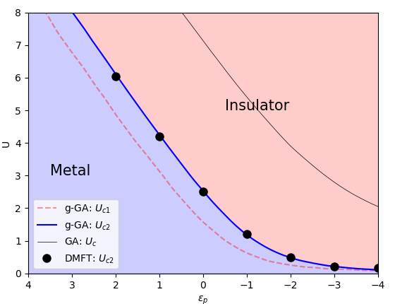
Figure 1: Paramagnetic phase diagram of the ALM on an infinite-coordination Bethe lattice, for $3$ electrons per site and $V=1$. The g-GA metal-insulator transition $U_{c2}$ and the end of the metal-insulator coexistence region $U_{c1}$ are marked in blue and red, respectively. The black dots are $U_{c2}$ values calculated with DMFT+CTQMC, at $T=0.01$. The gray line indicates the metal-insulator transition in bare GA.

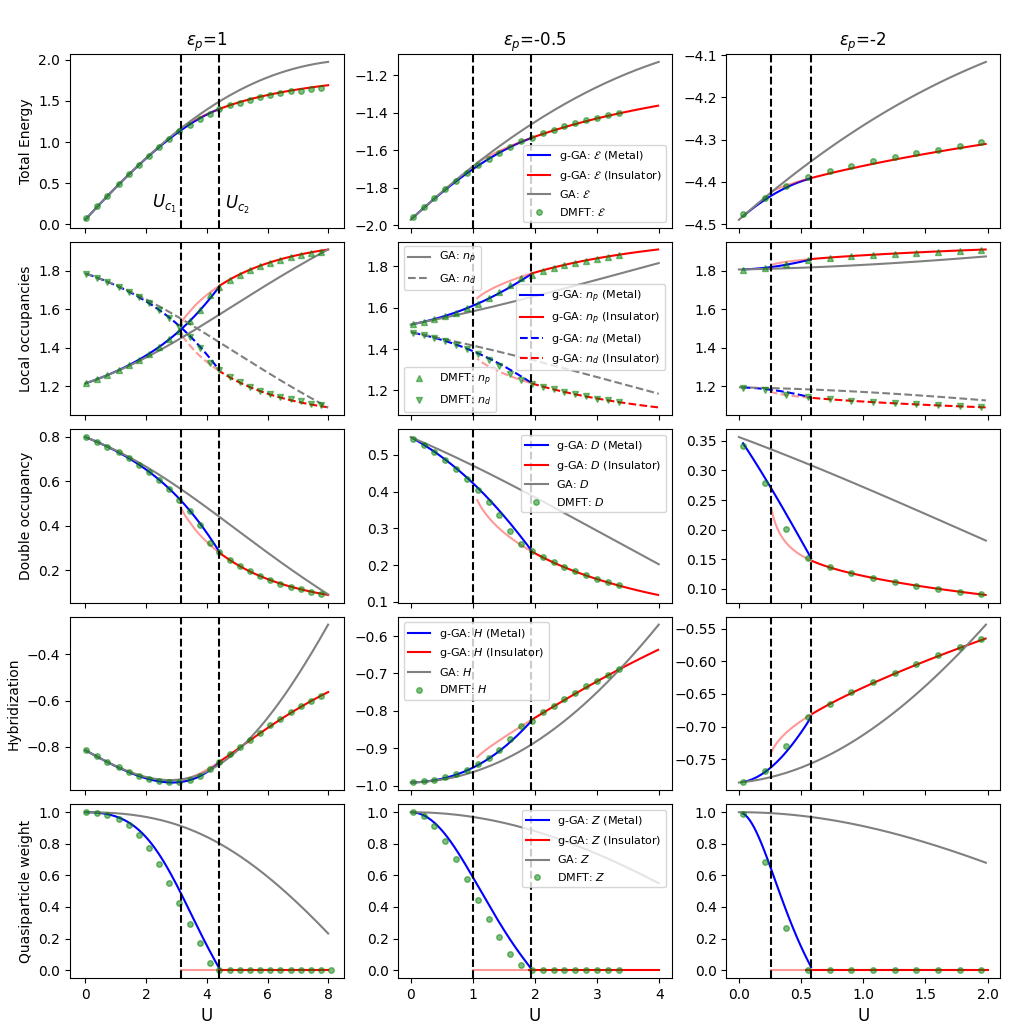
Figure 2: Behavior of the g-GA total energy $\mathcal{E}$, local occupancies $n_{p}=\langle\hat{n}_{pi}\rangle$ and $n_{d}=\langle\hat{n}_{di}\rangle$, $d$-electron double occupancy $D=\langle\hat{n}_{di\uparrow}\hat{n}_{di\downarrow}\rangle$, $p$-$d$ hybridization $H=\sum_{\sigma}\langle{d}^{\dagger}_{i\sigma}p_{i\sigma}\rangle+\text{c.c.}$ and $d$-electron quasiparticle weight $Z$, for the ALM on an infinite-coordination Bethe lattice, in comparison with DMFT and the bare GA. The DMFT data are computed with CTQMC, at $T=0.01$ for $\epsilon_{p}=1$ and $\epsilon_{p}=-0.5$ and at $T=0.02$ for $\epsilon_{p}=-2$. The vertical black dashed lines indicate $U_{c1}$ and $U_{c2}$.

Results.— In Fig. 1 we show the g-GA phase diagram of the ALM (in the paramagnetic phase) for total occupancy $\langle\hat{N}_{i}\rangle=3$. The g-GA results are compared with DMFT —with the continuous time quantum Monte Carlo (CTQMC) impurity solver [40, 41, 42], at temperature $T=0.01$— and with the bare GA. Our benchmark calculations show that the g-GA phase diagram is consistent with previous work [43, 44, 45] and in remarkable agreement with DMFT. As expected, both the g-GA method and the bare GA capture the fact that the Mott metal-insulator transition point $U_{c2}$ vanishes for $\varepsilon_{p}\rightarrow-\infty$ —corresponding to the limit where the $p$ degrees of freedom are gapped out. However, the interaction $U_{c}$ of the metal-insulator transition is largely overestimated within the GA, especially for $\epsilon_{p}\ll-1$. Note that the phase diagram for $\langle\hat{N}_{i}\rangle=1$ can be automatically inferred from our calculations above, as they are related to each other by a particle-hole transformation.

In Fig. 2 we show the behavior of the g-GA total energy $\mathcal{E}$, the occupancies $n_{p}=\langle\hat{n}_{pi}\rangle$ and $n_{d}=\langle\hat{n}_{di}\rangle$, the $d$-electron double occupancy $D=\langle\hat{n}_{di\uparrow}\hat{n}_{di\downarrow}\rangle$, the $p$-$d$ “hybridization energy” $H=\sum_{\sigma}\langle{d}^{\dagger}_{i\sigma}{p}^{\phantom{\dagger}}_{i\sigma}\rangle+\text{c.c.}$, and the $d$-electron quasiparticle weight:

$$Z =\left[1-\frac{\partial\Sigma^{\mathrm{g-GA}}}{\partial\omega}\right]^{-1}_{\omega=0}$$

$$=\frac{\left(l_{2}\,l_{3}\,r_{1}^{2}+l_{1}\,l_{3}\,r_{2}^{2}+l_{1}\,l_{2}\,r_{3}^{2}\right)^{2}}{l_{1}^{2}\,l_{3}^{2}\,r_{2}^{2}+l_{2}^{2}\left(l_{3}^{2}\,r_{1}^{2}+l_{1}^{2}\,r_{3}^{2}\right)}\,.$$ (15)

The g-GA results are shown in comparison with the bare GA and DMFT. While the GA solution is considered accurate only for weak interactions, we find that the agreement between g-GA and DMFT is remarkable for all observables, in all parameters regimes.

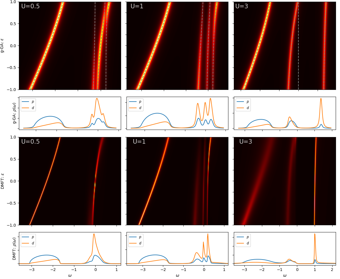
Figure 3: Energy-resolved spectral function and corresponding $p$ and $d$ local density of states $\rho(\omega)$, calculated with g-GA (upper panels) and DMFT+CTQMC (lower panels), for $\epsilon_{p}=-1$ and 3 values of $U$. The g-GA spectra is visualized using a small artificial smearing, $\Gamma=0.06$. The g-GA quasiparticle bands are indicated by gray dashed lines.

Let us now analyze the single-particle Green’s function. In Fig. 3 we consider $\epsilon_{p}=-1$ and 3 values of $U$, showing the total g-GA energy-resolved spectral function:

$$\mathcal{A}(k,\omega)=-\frac{1}{\pi}\text{Im}\mathrm{Tr}[\mathcal{G}(k,\omega)]$$ (16)

and the $p$ and $d$ local density of states. The DMFT spectra were obtained by performing analytical continuation with the maximum entropy method [46]. Interestingly, the g-GA captures systematically the main features of the DMFT spectra (including the Hubbard bands, and the hybridization between the $p$ and $d$ degrees of freedom). Note that, to interpret the behavior of the g-GA spectra, it is possible to exploit its relation with the bands of the QPH [Eq. (6)], previously discussed in the methods section. In particular, the relative position of the $p$ band with respect to the Fermi level is approximately encoded in the corresponding on-site energy $\epsilon_{p}^{*}=\epsilon_{p}-\mu$, while the positions of the $d$-electron low-energy and high-energy excitations are approximately encoded in the variational parameters $l_{a}$ ($a=1,2,3$).

A key fact emerging from our benchmark calculations is that the GA can overestimate $U_{c}$ dramatically (especially for $\epsilon_{p}\ll-1$), see Fig. 1. To explain this result we note that, by construction, the GA Mott transition occurs when the quasiparticle weight $Z=r^{2}$ vanishes, see Eq. (10). Therefore, the corresponding approximation to the Mott phase is such that $\langle{d}^{\dagger}_{i\sigma}{p}^{\phantom{\dagger}}_{i\sigma}\rangle_{\text{GA}}=0$, see Eq. (14). In other words, this method cannot describe simultaneously the Mott phase and the $p$-$d$ charge fluctuations. But this is unrealistic for the ALM, where the $p$-$d$ hybridization effects are generally very large, not only in the weakly-interacting regime, but also for $U\simeq U_{c2}$ and $U>U_{c2}$, see Figs. 2,3. Because of the variational principle, this results in a systematic overestimation of the total energy as we approach the Mott phase (see Fig. 2), causing an overestimation of the metal-insulator transition point. This point is documented in further detail in the supplemental material, where the GA overestimation of $U_{c}$ at $\epsilon_{p}\ll-1$ is explained in relation to a qualitative pathological behavior of the GA variational parameter $r$ in the narrow-bandwidth limit ($t\rightarrow 0)$.

Remarkably, since the g-GA captures the existence of the Hubbard bands, the right side of Eq. (11) never vanishes [31]. Therefore, similar to DMFT, $\langle{d}^{\dagger}_{i\sigma}{p}^{\phantom{\dagger}}_{i\sigma}\rangle_{\text{g-GA}}$ remains finite even in the Mott phase (see Eq. (13)). This shows that the ability of the g-GA of describing simultaneously the Mott physics and the $d$-$p$ hybridization is directly connected with its ability of describing the transfer of $d$-electron spectral weight to the Hubbard bands (which the bare GA lacks).

Conclusions.— We performed benchmark calculations of the ALM, showing that the g-GA provides us with results with accuracy comparable to DMFT, both for the ground-state and the spectral properties. In particular, we showed that the g-GA is capable of describing accurately the interplay between the Mott physics and the hybridization between correlated and itinerant degrees of freedom, while the GA cannot describe simultaneously these effects. This is particularly relevant for real-material calculations in combination with density functional theory [47, 17, 20, 48], where the correlated orbitals are generally very localized around their atomic positions [49, 50] —so that the interactions with their environment are mainly mediated by the itinerant modes (as in the ALM studied here). In fact, it is well possible that the limitation of the GA here uncovered explains why, in some cases, simulating the properties of real materials with the GA requires to use unphysically-large Hubbard $U$ [51], and suggests that multi-orbital implementations of the g-GA will resolve these problems.

From the computational standpoint, the g-GA is more expensive than the bare GA (as the bath of the EH contains additional degrees of freedom). On the other hand, its computational complexity remains much lower than DMFT. In fact, the g-GA requires to calculate only the ground state of a finite-size impurity model (while in DMFT it is necessary to calculate the spectra of an impurity model with an infinite bath). For example, in our DMFT calculations each CTQMC iteration (performed using $5\times 10^{8}$ Monte Carlo steps, in parallel, on 72 cores) required about 2 minutes of computational time. Instead, within our g-GA calculations each EH iteration (performed on a single core) required about 0.2-0.3 seconds. Note also that the difference in computational complexity between DMFT and g-GA grows exponentially as a function of the impurity size.

A particularly promising perspective is the possibility of solving the g-GA equations with hybrid quantum-classical frameworks [52], employing impurity solvers based on quantum algorithms such as variational quantum eigensolvers [53, 54, 55, 56]. In fact, within the g-GA, realizing such program for real-material applications may require devices consisting of only tens of qubits, while it has been estimated that quantum computers with at least 100 logical qubits will be necessary for applications within DMFT [57]. Furthermore, since the number of parameters characterizing the EH is finite, the recently-developed approach based on machine learning for the GA [58] will be applicable also to the g-GA, as we hope to show in future work. Note also that the g-GA can be equivalently formulated in terms of the rotationally-invariant slave-boson mean-field theory [31], which is based on an exact reformulation of the many-body problem. This line of interpretation may open the possibility of developing beyond-mean-field schemes, providing us with new routes for high-precision calculations.

References

- Kent and Kotliar [2018] P. R. C. Kent and G. Kotliar, Toward a predictive theory of correlated materials, Science 361, 348 (2018).
- Sun and Chan [2016] Q. Sun and G.-K.-L. Chan, Quantum embedding theories, Acc. Chem. Res. 49, 2705 (2016).
- Georges et al. [1996] A. Georges, G. Kotliar, W. Krauth, and M. J. Rozenberg, Dynamical mean-field theory of strongly correlated fermion systems and the limit of infinite dimensions, Rev. Mod. Phys. 68, 13 (1996).
- Anisimov and Izyumov [2010] V. Anisimov and Y. Izyumov, Electronic Structure of Strongly Correlated Materials (Springer, 2010).
- Maier et al. [2005] T. Maier, M. Jarrell, T. Pruschke, and M. H. Hettler, Quantum cluster theories, Rev. Mod. Phys. 77, 1027 (2005).
- Kotliar et al. [2001] G. Kotliar, S. Y. Savrasov, G. Pálsson, and G. Biroli, Cellular dynamical mean field approach to strongly correlated systems, Phys. Rev. Lett. 87, 186401 (2001).
- Lichtenstein and Katsnelson [2000] A. I. Lichtenstein and M. I. Katsnelson, Antiferromagnetism and -wave superconductivity in cuprates: A cluster dynamical mean-field theory, Phys. Rev. B 62, R9283 (2000).
- Potthoff et al. [2003] M. Potthoff, M. Aichhorn, and C. Dahnken, Variational cluster approach to correlated electron systems in low dimensions, Phys. Rev. Lett. 91, 206402 (2003).
- Senechal et al. [2000] D. Senechal, D. Perez, and M. Pioro-Ladriere, The spectral weight of the Hubbard model through cluster perturbation theory, Phys. Rev. Lett. 84, 522 (2000).
- Aichhorn et al. [2009] M. Aichhorn, L. Pourovskii, V. Vildosola, M. Ferrero, O. Parcollet, T. Miyake, A. Georges, and S. Biermann, Dynamical mean-field theory within an augmented plane-wave framework: Assessing electronic correlations in the iron pnictide LaFeAsO, Phys. Rev. B 80, 085101 (2009).
- Kotliar et al. [2006] G. Kotliar, S. Y. Savrasov, K. Haule, V. S. Oudovenko, O. Parcollet, and C. A. Marianetti, Electronic structure calculations with dynamical mean-field theory, Rev. Mod. Phys. 78, 865 (2006).
- Held et al. [2006] K. Held, A. Nekrasov, G. Keller, V. Eyert, N. Blümer, A. K. McMahan, R. T. Scalettar, T. Pruschke, V. I. Anisimov, and D. Vollhardt, Realistic investigations of correlated electron systems with LDA+DMFT, Phys. Stat. Sol. (B) 243, 2599 (2006).
- Zhao et al. [2012] J.-Z. Zhao, J.-N. Zhuang, X.-Y. Deng, Y. Bi, L.-C. Cai, Z. Fang, and X. Dai, Implementation of LDA+DMFT with the pseudo-potential-plane-wave method, Chin. Phys. B 21, 057106 (2012).
- Chen et al. [2015] L.-Q. Chen, L.-D. Chen, S. V. Kalinin, G. Klimeck, S. K. Kumar, J. Neugebauer, and I. Terasaki, Design and discovery of materials guided by theory and computation, npj Computational Materials 1, 15007 (2015).
- Adler et al. [2018] R. Adler, C.-J. Kang, C.-H. Yee, and G. Kotliar, Correlated materials design: prospects and challenges, Reports on Progress in Physics 82, 012504 (2018).
- Gutzwiller [1965] M. C. Gutzwiller, Correlation of Electrons in a Narrow Band, Phys. Rev. 137, A1726 (1965).
- Deng et al. [2009] X.-Y. Deng, L. Wang, X. Dai, and Z. Fang, Local density approximation combined with Gutzwiller method for correlated electron systems: Formalism and applications, Phys. Rev. B 79, 075114 (2009).
- Ho et al. [2008] K. M. Ho, J. Schmalian, and C. Z. Wang, Gutzwiller density functional theory for correlated electron systems, Phys. Rev. B 77, 073101 (2008).
- Schickling et al. [2011] T. Schickling, F. Gebhard, and J. Bünemann, Antiferromagnetic order in multiband Hubbard models for iron pnictides, Phys. Rev. Lett. 106, 146402 (2011).
- Lanatà et al. [2015] N. Lanatà, Y.-X. Yao, C.-Z. Wang, K.-M. Ho, and G. Kotliar, Phase diagram and electronic structure of praseodymium and plutonium, Phys. Rev. X 5, 011008 (2015).
- Lanatà et al. [2012] N. Lanatà, H. U. R. Strand, X. Dai, and B. Hellsing, Efficient implementation of the Gutzwiller variational method, Phys. Rev. B 85, 035133 (2012).
- Bünemann and Gebhard [2007] J. Bünemann and F. Gebhard, Equivalence of Gutzwiller and slave-boson mean-field theories for multiband Hubbard models, Phys. Rev. B 76, 193104 (2007).
- Lanatà et al. [2008] N. Lanatà, P. Barone, and M. Fabrizio, Fermi-surface evolution across the magnetic phase transition in the Kondo lattice model, Phys. Rev. B 78, 155127 (2008).
- Frésard and Wölfle [1992] R. Frésard and P. Wölfle, Unified slave boson representation of spin and charge degrees of freedom for strongly correlated fermi systems, International Journal of Modern Physics B 06, 685 (1992).
- Lechermann et al. [2007] F. Lechermann, A. Georges, G. Kotliar, and O. Parcollet, Rotationally invariant slave-boson formalism and momentum dependence of the quasiparticle weight, Phys. Rev. B 76, 155102 (2007).
- Lanatà et al. [2017] N. Lanatà, Y.-X. Yao, X. Deng, V. Dobrosavljević, and G. Kotliar, Slave Boson Theory of Orbital Differentiation with Crystal Field Effects: Application to UO2, Phys. Rev. Lett. 118, 126401 (2017).
- Knizia and Chan [2012] G. Knizia and G. K.-L. Chan, Density matrix embedding: A simple alternative to dynamical mean-field theory, Phys. Rev. Lett. 109, 186404 (2012).
- Fertitta and Booth [2018] E. Fertitta and G. H. Booth, Rigorous wave function embedding with dynamical fluctuations, Phys. Rev. B 98, 235132 (2018).
- Ayral et al. [2017] T. Ayral, T.-H. Lee, and G. Kotliar, Dynamical mean-field theory, density-matrix embedding theory, and rotationally invariant slave bosons: A unified perspective, Phys. Rev. B 96, 235139 (2017).
- Lee et al. [2019] T.-H. Lee, T. Ayral, Y.-X. Yao, N. Lanatà, and G. Kotliar, Rotationally invariant slave-boson and density matrix embedding theory: Unified framework and comparative study on the one-dimensional and two-dimensional Hubbard model, Phys. Rev. B 99, 115129 (2019).
- Lanatà et al. [2017] N. Lanatà, T.-H. Lee, Y.-X. Yao, and V. Dobrosavljević, Emergent Bloch excitations in Mott matter, Phys. Rev. B 96, 195126 (2017).
- Metzner and Vollhardt [1989] W. Metzner and D. Vollhardt, Correlated lattice fermions in dimensions, Phys. Rev. Lett. 62, 324 (1989).
- [33] Supplemental material: Lagrange formulation of the g-GA in multi-orbital case (including general analytical expression for the g-GA self energy) and details about GA pathology in narrow-band limit .
- Guerci et al. [2019] D. Guerci, M. Capone, and M. Fabrizio, Exciton Mott transition revisited, Phys. Rev. Materials 3, 054605 (2019).
- Jain and Anderson [2009] J. K. Jain and P. W. Anderson, Beyond the fermi liquid paradigm: Hidden fermi liquids, Proceedings of the National Academy of Sciences 106, 9131 (2009).
- Savrasov et al. [2006] S. Y. Savrasov, K. Haule, and G. Kotliar, Many-body electronic structure of americium metal, Phys. Rev. Lett. 96, 036404 (2006).
- Savrasov et al. [2005] S. Y. Savrasov, V. Oudovenko, K. Haule, D. Villani, and G. Kotliar, Interpolative approach for solving the Anderson impurity model, Phys. Rev. B 71, 115117 (2005).
- Sakai et al. [2016] S. Sakai, M. Civelli, and M. Imada, Hidden-fermion representation of self-energy in pseudogap and superconducting states of the two-dimensional Hubbard model, Phys. Rev. B 94, 115130 (2016).
- Bünemann et al. [2003] J. Bünemann, F. Gebhard, and R. Thul, Landau-Gutzwiller quasiparticles, Phys. Rev. B 67, 075103 (2003).
- Werner et al. [2006] P. Werner, A. Comanac, L. de’ Medici, M. Troyer, and A. J. Millis, Continuous-time solver for quantum impurity models, Phys. Rev. Lett. 97, 076405 (2006).
- Gull et al. [2011] E. Gull, A. J. Millis, A. I. Lichtenstein, A. N. Rubtsov, M. Troyer, and P. Werner, Continuous-time Monte Carlo methods for quantum impurity models, Rev. Mod. Phys. 83, 349 (2011).
- Haule [2007] K. Haule, Quantum Monte Carlo impurity solver for cluster dynamical mean-field theory and electronic structure calculations with adjustable cluster base, Phys. Rev. B 75, 155113 (2007).
- Amaricci et al. [2017] A. Amaricci, L. de’ Medici, and M. Capone, Mott transitions with partially filled correlated orbitals, EPL (Europhysics Letters) 118, 17004 (2017).
- Zaanen et al. [1985] J. Zaanen, G. A. Sawatzky, and J. W. Allen, Band gaps and electronic structure of transition-metal compounds, Phys. Rev. Lett. 55, 418 (1985).
- Sordi et al. [2007] G. Sordi, A. Amaricci, and M. J. Rozenberg, Metal-insulator transitions in the periodic anderson model, Phys. Rev. Lett. 99, 196403 (2007).
- Jarrell and Gubernatis [1996] M. Jarrell and J. E. Gubernatis, Bayesian inference and the analytic continuation of imaginary-time quantum Monte Carlo data, Physics Reports 269, 133 (1996).
- Anisimov et al. [1997a] V. I. Anisimov, A. I. Oteryaev, M. A. Korotin, A. O. Anokhin, and G. Kotliar, First-principles calculations of the electronic structure and spectra of strongly correlated systems: dynamical mean-field theory, J. Phys. Condens. Matter 9, 7359 (1997a).
- Anisimov et al. [1997b] V. I. Anisimov, F. Aryasetiawan, and A. I. Lichtenstein, First-principles calculations of the electronic structure and spectra of strongly correlated systems: the LDA+U method, J. Phys. Condens. Matter 9, 767 (1997b).
- Haule et al. [2010] K. Haule, C.-H. Yee, and K. Kim, Dynamical mean-field theory within the full-potential methods: Electronic structure of , , and , Phys. Rev. B 81, 195107 (2010).
- Lechermann et al. [2006] F. Lechermann, A. Georges, A. Poteryaev, S. Biermann, M. Posternak, A. Yamasaki, and O. K. Andersen, Dynamical mean-field theory using Wannier functions: A flexible route to electronic structure calculations of strongly correlated materials, Phys. Rev. B 74, 125120 (2006).
- Lanatà et al. [2019] N. Lanatà, T.-H. Lee, Y.-X. Yao, V. Stevanović, and V. Dobrosavljević, Connection between Mott physics and crystal structure in a series of transition metal binary compounds, npj Comput. Mater. 5, 30 (2019).
- Yao et al. [2021] Y.-X. Yao, F. Zhang, C.-Z. Wang, K.-M. Ho, and P. P. Orth, Gutzwiller hybrid quantum-classical computing approach for correlated materials, Phys. Rev. Research 3, 013184 (2021).
- McClean et al. [2016] J. R. McClean, J. Romero, R. Babbush, and A. Aspuru-Guzik, The theory of variational hybrid quantum-classical algorithms, New Journal of Physics 18, 023023 (2016).
- O’Malley et al. [2016] P. J. J. O’Malley, R. Babbush, I. D. Kivlichan, J. Romero, J. R. McClean, R. Barends, J. Kelly, P. Roushan, A. Tranter, N. Ding, et al., Scalable quantum simulation of molecular energies, Physical Review X 6, 031007 (2016).
- Kandala et al. [2017] A. Kandala, A. Mezzacapo, K. Temme, M. Takita, M. Brink, J. M. Chow, and J. M. Gambetta, Hardware-efficient variational quantum eigensolver for small molecules and quantum magnets, Nature 549, 242 (2017).
- Romero et al. [2018] J. Romero, R. Babbush, J. R. McClean, C. Hempel, P. J. Love, and A. Aspuru-Guzik, Strategies for quantum computing molecular energies using the unitary coupled cluster ansatz, Quantum Science and Technology 4, 014008 (2018).
- Bauer et al. [2016] B. Bauer, D. Wecker, A. J. Millis, M. B. Hastings, and M. Troyer, Hybrid quantum-classical approach to correlated materials, Phys. Rev. X 6, 031045 (2016).
- Rogers et al. [2021] J. Rogers, T.-H. Lee, S. Pakdel, W. Xu, V. Dobrosavljević, Y.-X. Yao, O. Christiansen, and N. Lanatà, Bypassing the computational bottleneck of quantum-embedding theories for strong electron correlations with machine learning, Phys. Rev. Research 3, 013101 (2021).