Abstract

The theoretical calculation for pseudo–scalars hadronic decays $K\to\pi a$ is reviewed. While one-loop penguin contributions are usually considered, tree-level processes have most often been overlooked in literature. Following the Lepage–Brodsky approach the tree-level contribution to the charged and neutral pseudo–scalar decay in ALP is estimated. Assuming generic ALP couplings to SM fermions, the latest NA62/E949 results for the $K^{+}\to\pi^{+}a$ decay and the present/future KOTO results for the $K^{0}_{L}\to\pi^{0}a$ decay are used to provide updated bounds on the ALP–fermion Lagrangian sector. Finally, the interplay between the tree-level and one-loop contributions is investigated.

1 Introduction

Light pseudoscalar particles naturally arise in many extensions of the Standard Model (SM) of particle physics. In particular they are a common feature of any BSM model endowed with (at least) a global $U(1)$ symmetry spontaneously broken at some high scale $f_{a}\gg v$. Small breaking terms of the global symmetry are then necessary in order to provide a mass term, $m_{a}\ll f_{a}$, to the generated pseudo Nambu-Goldstone boson (pNGB). Therefore, it may be not inconceivable that the first hint of new physics at (or above) the TeV scale could be the discovery of a light pseudoscalar state.

Sharing a common nature with the QCD axion [1, 2, 3], these class of pNGBs are generically referred to as Axion-Like Particles (ALPs). The key difference between the QCD axion and a generic ALP can be summarized in the well-known constraints [3]:

$$m_{a}f_{a}\approx m_{\pi}f_{\pi}$$ (1)

that bounds the QCD axion mass and the $U(1)_{PQ}$ symmetry breaking scale via QCD instanton effects. Present bounds on the reference QCD invisible-axion models, like the DNSZ and KVSZ ones [4, 5, 6, 7], force the axion mass to be typically in the sub-eV range with the symmetry breaking scale $f_{a}\gtrsim 10^{11}$ GeV. In a generic ALP framework, instead, one can assume the ALP mass being determined by some unspecified UV physics, besides the usual QCD anomalous contribution, and then relation in Eq. (1) has not to be enforced. Consequently, the ALP mass and the $U(1)_{PQ}$ breaking scale $f_{a}$ can be taken as independent parameters and in the range phenomenologically of interest at present or near future colliders. In this context, a generic ALP can be seen as the generalization of non fine-tuned axion models, and permit to look without prejudice to all the possible light pseudo–scalar signatures in Cosmology, Astro–Particle and Collider physics.

The ALP parameter space has been intensively explored in several terrestrial facilities, covering a wide energy range  [8, 9, 10, 11, 12, 13, 14, 15], as well as by many astrophysical and cosmological probes [16, 17, 18]. The synergy of these experimental searches allows to access several orders of magnitude in ALP masses and couplings, cf. e.g. Ref. [19] and references therein. While astrophysics and cosmology impose severe constraints on ALPs in the sub-KeV mass range, the most efficient probes of weakly-coupled particles in the MeV-GeV range come from experiments acting on the precision frontier [20]. Fixed-target facilities such as E949 [21, 22, 23], NA62 [24, 25] and KOTO [26] and the proposed SHiP [27] and DUNE [28] experiments can be very efficient to constrain long-lived particles. Furthermore, the rich ongoing research program in the $B$-physics experiments at LHCb [29, 30] and the $B$-factories [31, 32, 33, 34, 35, 36, 37, 38, 15] offers several possibilities to probe yet unexplored ALP couplings.

The main goal of this letter, is the detailed analysis of the $K\to\pi a$ decays, in view of the recent NA62 updated measurement and the foreseen updates of the KOTO results. While one-loop penguin contributions are usually considered [33, 34, 38], the tree-level process contributing to the decay has most often been overlooked in literature typically for two reasons. First of all one expects the penguin diagrams to dominate, despite the loop suppression, being proportional to the mass of the virtual top quark running in the loop. However, in the $K\to\pi a$ case, one has to take into account that the top–loop contribution is CKM suppressed compared to the tree-level roughly by a factor $\lambda^{4}$, and this can partially compensate for the top mass enhancement. The second reason is because the tree-level contributions show a much more complicated hadronization structure, being the ALP emitted “inside” the initial or final meson and so require a dedicated treatment [39, 40]. An alternative approach for calculating $K\to\pi a$ decays using chiral perturbation theory can be found, for example, in [41, 42].

The letter is organized as follows. In Sec. 2 the effective Lagrangian describing the flavor-conserving interactions between the ALP and SM fermions up to dimension five is introduced. In Sec. 3 the tree-level contribution to the $K\to\pi a$ decay is going to be thoroughly discussed. Then, the one-loop penguin contributions are shortly reviewed. Finally, in Sec. 4 the interplay between the tree-level and one-loop contributions to the $K\to\pi a$ Branching Ratio is thoroughly discussed. Concluding remarks are deferred to Sec. 5.

2 Effective ALP-SM Fermion Lagrangian

The most general effective Lagrangian describing ALP interactions with SM quarks, including operators up to dimension five, reads:

$$\delta\mathcal{L}^{a}_{\mathrm{eff}} = \frac{\partial_{\mu}a}{f_{a}}\left[\overline{U}\,\gamma^{\mu}\left(C^{(u)}_{L}P_{L}\,+\,C^{(u)}_{R}P_{R}\right)\,U\,+\,\overline{D}\,\gamma^{\mu}\left(C^{(d)}_{L}P_{L}\,+\,C^{(d)}_{R}P_{R}\right)\,D\right]$$ (2)

where $f_{a}$ is the $U(1)_{PQ}$ symmetry breaking scale, $U$ and $D$ the SM up and down flavour triplets and $C_{L,R}$ are general $3\times 3$ hermitian matrices. One can, however, heavily reduce the number of independent parameters imposing that the only source of flavor–violation in the model arises through the SM Yukawa couplings. Therefore, once the Minimal Flavor Violation (MFV) ansatz is assumed, the ALP–quarks Lagrangian becomes

$$\delta\mathcal{L}^{a,MFV}_{\mathrm{eff}} = -\frac{\partial_{\mu}a}{2f_{a}}\sum_{i=quarks}c_{i}\,\overline{\psi}_{i}\gamma^{\mu}\gamma_{5}\,\psi_{i}\,=\,i\frac{a}{f_{a}}\sum_{i=quarks}c_{i}m_{i}\,\overline{\psi}_{i}\gamma_{5}\,\psi_{i}$$ (3)

and depends only on six independent flavor diagonal couplings, $c_{i}$, once the vector fermionic current conservation is implied. Therefore, in the MFV framework, flavor–violating ALP couplings can be generated only at loop level, and is proportional to the SM CKM mixings. To further reduce the number of independent parameters, one can additionally assume universal couplings for the up and down sectors, in the following denoted as $c_{\uparrow}$ and $c_{\downarrow}$, respectively. It may not be unconceivable, in fact, that an hypothetical UV–complete model provides different universal PQ charges to the up and down quark sectors [43, 44, 45]. Finally, in the most constrained scenario, one can assume a unique ALP-fermion coupling, often denoted as $c_{a\Phi}$ in the literature, as it originates from the dimension five ALP-Higgs operator

$$\mathcal{O}_{a\Phi}\equiv i\,\frac{\partial_{\mu}a}{f_{a}}\left(\Phi\stackrel{{\scriptstyle\leftrightarrow}}{{D}}_{\mu}\Phi\right),$$ (4)

once the Higgs field is accordingly redefined [46]. These additional assumptions will become useful in simplifying the phenomenological analysis and their implication will be discussed in Sec. 4. A general discussion on tree–level flavor–violating ALPs couplings to fermions can be found in [15], while for a recent analysis on CP–violating ALP couplings to fermions one is referred, for example, to [47].

It might be useful, for simplifying intermediate calculations and explicitly showing the mass dependence of ALP-fermion couplings, to write the effective Lagrangian of Eq. (3) in the “Yukawa” basis instead of the “derivative” one. The two versions of the effective Lagrangian are equivalent up to operators of $O(1/f_{a}^{2})$.

3 Meson Hadronization in Flavor Changing Processes

Using the effective Lagrangian, implemented with the flavor conserving assumption, of Eq. 3 one can calculate the hadronic decay rates of mesons in ALPs. In the following, due to their experimental relevance, the pseudo-scalar meson hadronic decays:

$$K^{+}\rightarrow\pi^{+}\,a\qquad{\rm and}\qquad K^{0}_{L}\rightarrow\pi^{0}\,a$$ (5)

will be mainly considered, with the ALP sufficiently long-living to escape the detector without decaying or decaying into invisible channels. In such a case the only possible ALP signature is its missing energy/momentum. In the following, with $M_{K^{+,0}},P_{K^{+,0}}$ and $M_{\pi^{+,0}},P_{\pi^{+,0}}$ the mass and 4–momentum of the $K^{+,0}$ and $\pi^{+,0}$ mesons will be denoted, respectively, while the ALP mass and 4–momentum will be indicated with $m_{a}$ and $k_{a}$.

The processes at hand receive contributions both from tree–level and one–loop diagrams. Typically, for this kind of processes, the one–loop penguin diagrams with a top virtual exchange give the dominant contribution, as the $m_{t}/m_{q,ext}$ ratio largely compensate the loop suppression factor. The tree–level and one–loop decay channels involve, however, quite different hadronization structures that have to be properly taken into account for correctly comparing the relative contributions to the $K$ decay rates. In the following subsections it is briefly illustrated how to handle both contributions in a simple way, applying different hadronization methods [39, 40, 49].

3.1 The tree-level s-channel process

Charged pseudo-scalar meson decays proceed through the s–channel tree-level diagrams of Fig. 1. Here only the diagrams where the ALP is emitted from the $K^{+}$ meson are shown, the ones where the ALP is emitted from the $\pi^{+}$ follow straightforwardly. The tree-level diagram with the ALP emitted from the $W^{+}$ internal line automatically vanishes, being the WW-ALP coupling proportional to the fully antisymmetric 4D tensor. The hadronization of the s–channel can be done following the Lepage–Brodsky technique [39, 40]. Leptonic pseudo–scalar decays, $\mathcal{P}\to\ell\,\nu_{\ell}\,a$, deserve a similar treatment and have been derived in [50, 51]. Let’s recall briefly the notation.

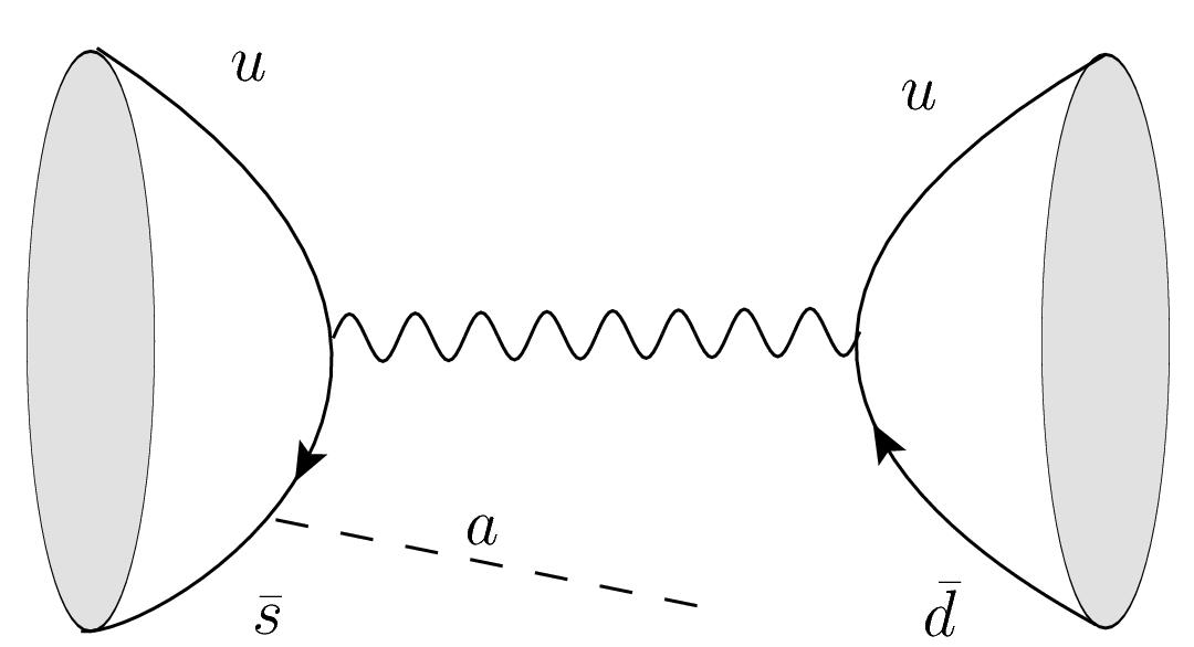
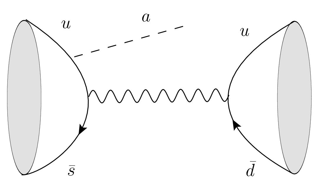
Figure 1: Tree level contributions to the $K^{+}\rightarrow\pi^{+}\,a$ amplitude, with the ALP emitted from the $K^{+}$ meson. Diagrams where the ALP is emitted from the $\pi^{+}$ quarks are straightforward.

The parent meson $K^{+}$ constituent quarks annihilate into a virtual W boson that then produces the final $\pi^{+}$ meson partons. The hadronic process can be factorized as $\bra{\pi^{+}}\bar{u}\,\Gamma_{(\pi)}\,d\ket{0}\bra{0}\bar{s}\,\Gamma_{(K)}\,u\ket{K^{+}}$ with the operator insertion $\Gamma_{(\pi)}\otimes\Gamma_{(K)}$ being $\gamma^{\mu}P_{L}\otimes\Gamma_{\mu}$ or $\Gamma^{\prime}_{\mu}\otimes\gamma^{\mu}P_{L}$ depending if the ALP is emitted by the initial or final mesons, with

$$\Gamma_{\mu} = \frac{4G_{F}}{\sqrt{2}}V^{*}_{us}V_{ud}\left(\frac{c_{s}\,m_{s}}{f_{a}}\,\gamma_{5}\,\frac{\not{k}_{a}-\not{p}_{\bar{s}}+m_{s}}{m_{a}^{2}-2k_{a}\cdot p_{\bar{s}}}\,\gamma_{\mu}P_{L}\,-\,\frac{c_{u}\,m_{u}}{f_{a}}\,\gamma_{\mu}P_{L}\,\frac{\not{k}_{a}-\not{p}_{u}-m_{u}}{m_{a}^{2}-2k_{a}\cdot p_{u}}\,\gamma_{5}\right)$$ (6)

$$\Gamma^{\prime}_{\mu} = \frac{4G_{F}}{\sqrt{2}}V^{*}_{us}V_{ud}\left(\frac{c_{u}\,m_{u}}{f_{a}}\,\gamma_{5}\,\frac{\not{k}_{a}+\not{p}^{\prime}_{u}+m_{u}}{m_{a}^{2}-2k_{a}\cdot p^{\prime}_{u}}\,\gamma_{\mu}P_{L}\,\,-\,\frac{c_{d}\,m_{d}}{f_{a}}\,\gamma_{\mu}P_{L}\,\frac{\not{k_{a}}+\not{p}^{\prime}_{\bar{d}}-m_{d}}{m_{a}^{2}-2k_{a}\cdot p^{\prime}_{\bar{d}}}\,\gamma_{5}\right).$$ (7)

In Eqs. (6) and (7) with $p_{s},p_{u}$ and $p^{\prime}_{d},p^{\prime}_{u}$ the quark momenta of the initial and final meson are denoted, respectively. In deriving these Equations the “Yukawa” basis for the ALP-SM quark couplings has been explicitly used, providing a simpler $\gamma$ structure and showing explicitly the mass dependence of the quark-ALP couplings.

The vector and axial matrix elements can be parameterized in terms of the meson decay constants $f_{K}$ and $f_{\pi}$ as:

$$\bra{0}\bar{s}\,\gamma^{\mu}\,\gamma_{5}\,u\ket{K^{+}}=if_{K}P_{K}^{\mu}\qquad,\qquad\bra{0}\bar{s}\,\gamma^{\mu}\,u\ket{K^{+}}=0$$ (8)

$$\bra{0}\bar{d}\,\gamma^{\mu}\,\gamma_{5}\,u\ket{\pi^{+}}=if_{\pi}P_{\pi}^{\mu}\,\,\,\qquad,\qquad\,\bra{0}\bar{d}\,\gamma^{\mu}\,u\ket{\pi^{+}}=0\,.$$ (9)

To compute the $\bra{0}\bar{s}\,\Gamma_{\mu}\,u\,\ket{K^{+}}$ and $\bra{\pi^{+}}\bar{u}\,\Gamma^{\prime}_{\mu}\,d\,\ket{0}$ hadronic matrix elements, one has to assume a model for describing the effective quark–antiquark distribution inside the meson emitting the ALP. Following [39, 40, 50], the ground state of a meson $M$ is parameterized with the wave–function

$$\Psi_{M}(x)=\frac{1}{4}\phi_{M}(x)\gamma^{5}(\not{P}_{M}+g_{M}(x)M_{M}),$$ (10)

where ${P}_{M}$ and $M_{M}$ denote the momentum and the mass of the meson emitting the ALP. In Eq. (10), with $x$ one typically denotes the fraction of the momentum carried by the heaviest quark in the meson. The function $\phi_{M}(x)$ describes the meson quarks momenta distribution, that for heavy and light mesons reads, respectively:

$$\phi_{H}(x)\propto\left[\frac{\xi^{2}}{1-x}+\frac{1}{x}-1\right]^{-2}\qquad,\qquad\phi_{L}(x)\propto x(1-x)\,,$$ (11)

with the normalization fixed such that:

$$\int_{0}^{1}dx\,\phi_{M}(x)=1.$$ (12)

The parameter $\xi$ in $\phi_{H}(x)$ is a small parameter typically of $O(m_{q}/m_{Q})$, being $q$ and $Q$ the light and heavy quark in the meson. The mass function $g_{M}(x)$ is usually taken to be a constant varying from $g_{H}(x)\approx 1$ and $g_{L}(x)\ll 1$ for a heavy or a light meson, respectively. The hadronic matrix element can then be obtained by integrating over the momentum fraction $x$ the trace of the $\Gamma^{\mu}$ amplitude over the meson wave–function $\Psi_{M}(x)$:

$$\bra{0}\bar{Q}\,\Gamma^{\mu}\,q\ket{M}\equiv if_{M}\int_{0}^{1}dx\,\mathrm{Tr}\left[\Gamma^{\mu}\Psi_{M}(x)\right]\,.$$ (13)

In Eqs. (10-13), a slightly different notation with respect to the cited literature is used, in particular, as for weak decays colors are left unchanged, all the color matrices/traces have been removed from scratch. Moreover, the functions $\Phi_{M}(x)$ have been normalized to one, in such a way that in Eq. (13) the mesonic form factor can be explicitly factorized.

By inserting Eqs. (6-7) into Eq. (13), and making the following assignments for the initial and final quark momenta:

$$p_{\bar{s}} = xP_{K}\qquad,\qquad p_{u}=(1-x)P_{K}$$

$$p^{\prime}_{\bar{d}} = xP_{\pi}\qquad\,,\,\qquad p^{\prime}_{u}=(1-x)P_{\pi}$$

one obtains the following decay amplitudes for the $K^{+}$-ALP and $\pi^{+}$-ALP emission processes:

$$\mathcal{M}_{K^{+}} = \frac{G_{F}}{\sqrt{2}}(V^{*}_{us}V_{ud})\,f_{K}\,f_{\pi}\,(k_{a}\cdot P_{\pi})\frac{M_{K}}{f_{a}}\,\times\,$$

$$\hskip 21.33955pt\times\int^{1}_{0}\left\{\frac{c_{s}\,m_{s}\,\theta(x-\delta^{K}_{a})}{m_{a}^{2}-2\,x\,k_{a}\cdot P_{K}}-\frac{c_{u}\,m_{u}\,\theta(1-x-\delta^{K}_{a})}{m_{a}^{2}-2\,(1-x)\,k_{a}\cdot P_{K}}\right\}\,\phi_{K}(x)\,g_{K}(x)\,dx$$

$$\mathcal{M}_{\pi^{+}} = \frac{G_{F}}{\sqrt{2}}(V^{*}_{us}V_{ud})\,f_{K}\,f_{\pi}\,(k_{a}\cdot P_{K})\frac{M_{\pi}}{f_{a}}\,\times\,$$

$$\hskip 21.33955pt\times\int^{1}_{0}\left\{\frac{c_{d}\,m_{d}\,\theta(x-\delta^{\pi}_{a})}{m_{a}^{2}-2\,x\,k_{a}\cdot P_{\pi}}-\frac{c_{u}\,m_{u}\,\theta(1-x-\delta^{\pi}_{a})}{m_{a}^{2}-2\,(1-x)\,k_{a}\cdot P_{\pi}}\right\}\,\phi_{\pi}(x)\,g_{\pi}(x)\,dx$$

with $\delta^{M}_{a}=m_{a}^{2}/(2k\cdot P_{M})$ an explicit cutoff introduced in the fractional momentum to remove the unphysical singularities appearing in the integrals. The result in Eq. (3.1) is in agreement with the decay amplitude for $B^{\pm}\to\ell\,\bar{\nu}_{\ell}\,a$ calculated in [50] once $c_{u}=c_{s}=1$ is assumed, the pion hadronic current is replaced by the leptonic one, and K quantities replaced by the corresponding B meson ones. Eqs. (3.1) and (3.1) represent the main result of this section.

Few comments are in order. To numerically evaluate the $K^{+}\to\pi^{+}\,a$ branching ratio one has to assume a specific form of the hadronic functions $\phi_{K}(x)$, $g_{K}(x)$, $\phi_{\pi}(x)$ and $g_{\pi}(x)$, and assign a low energy meaning to the quark masses. This, inevitably, introduces some model dependence in the calculation. To have an order of magnitude estimate of the $\mathcal{M}_{K^{+}}$ amplitude, one can consider the two extreme cases and treat the K-meson either as a light meson (i.e. assuming an exact global $SU(3)$ symmetry) or as an heavy meson (i.e. $m_{s}\gg m_{u},m_{d}$). In the light meson approximation, substituting the light quarks with the corresponding partons, i.e. $\hat{m}_{s}=\hat{m}_{u}=M_{K}/2$, one obtains, for a massless ALP:

$$\mathcal{M}^{L}_{K^{+}}\approx-\frac{3\,G_{F}\,f_{K}\,f_{\pi}}{4\sqrt{2}}(V^{*}_{us}V_{ud})\frac{M^{2}_{K}}{f_{a}}\,g_{K}\,\left(c_{s}-c_{u}\right)\,.$$ (16)

Conversely, in the heavy meson approximation, one can assume $\hat{m}_{u}=\xi M_{K}$ and $\hat{m}_{s}=(1-\xi)M_{K}$, with $\xi=m_{u}/m_{s}$. Moreover, approximating $\phi_{K}(x)\approx\delta(1-x-\xi)$ as suggested in [52], one obtains, in the $m_{a}=0$ limit:

$$\mathcal{M}^{H}_{K^{+}}\approx-\frac{G_{F}\,f_{K}\,f_{\pi}}{2\sqrt{2}}(V^{*}_{us}V_{ud})\frac{M^{2}_{K}}{f_{a}}\,g_{K}\,\left(c_{s}-c_{u}\right)\,.$$ (17)

From the approximate formulas of Eq. (16) and (17) one can estimate roughly the order of magnitude of the uncertainties introduced in the calculation by the hadronization procedure for the K meson. To reproduce the numerical results of the following section, an intermediate approach will be, instead, considered: the heavy meson function will be used, with the two partons defined as $\hat{m}_{u}=m_{u}+\Lambda$ and $\hat{m}_{s}=m_{s}+\Lambda$ with $\Lambda=(M_{K}-m_{u}-m_{s})/2$ a parameter of order $\Lambda_{QCD}$. Conversely, for the estimation of the $\mathcal{M}_{\pi}$ amplitude, one can safely assume to parametrize the pion using the light meson wave-function. If one take $g_{\pi}(x)\approx 0$, as customarily suggested in the literature the pion contribution automatically vanishes. A conservative estimate can however be obtained by setting, for example, $g_{\pi}/g_{K}\approx M_{\pi}/M_{K}$, which predicts the following upper bound to the ratio

$$R_{\pi K}=\left|\frac{\mathcal{M}_{\pi^{+}}}{\mathcal{M}_{K^{+}}}\right|\lesssim\left(\frac{M_{\pi}}{M_{K}}\right)^{3}\simeq 1.\times 10^{-2}\,.$$

For this reason, even in the numerical calculation one can neglect the ALP-$\pi$ emission as expected on a general ground, once same order ALP couplings to $u,d$ and $s$ quarks are assumed.

Finally, from Eqs. (16) and (17) it appears evident the presence of an “accidental” cancelation if $c_{s}=c_{u}$ is assumed. This cancellation is still partially at work even when the full $\phi_{K}(x)$ is used and indicates a possible underestimation of the $\mathcal{M}_{K}$ amplitude (and consequently on the ALP-quark coupling limits) in a “universal” ALP–SM quark coupling scenario compared to the general case.

3.2 The tree-level t-channel process

Neutral pseudo-scalar meson decays proceed through the t–channel tree-level diagrams of Fig. 2. Here only the diagrams where the ALP is emitted from the $K^{0}$ meson are shown, the ones where the ALP is emitted from the $\pi^{0}$ follow straightforwardly. The tree-level diagram with the ALP emitted from the $W^{+}$ internal line automatically vanishes, as for the s–channel case. The hadronization of the t–channel can be done along the lines depicted in [39, 40].

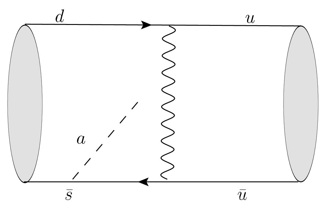
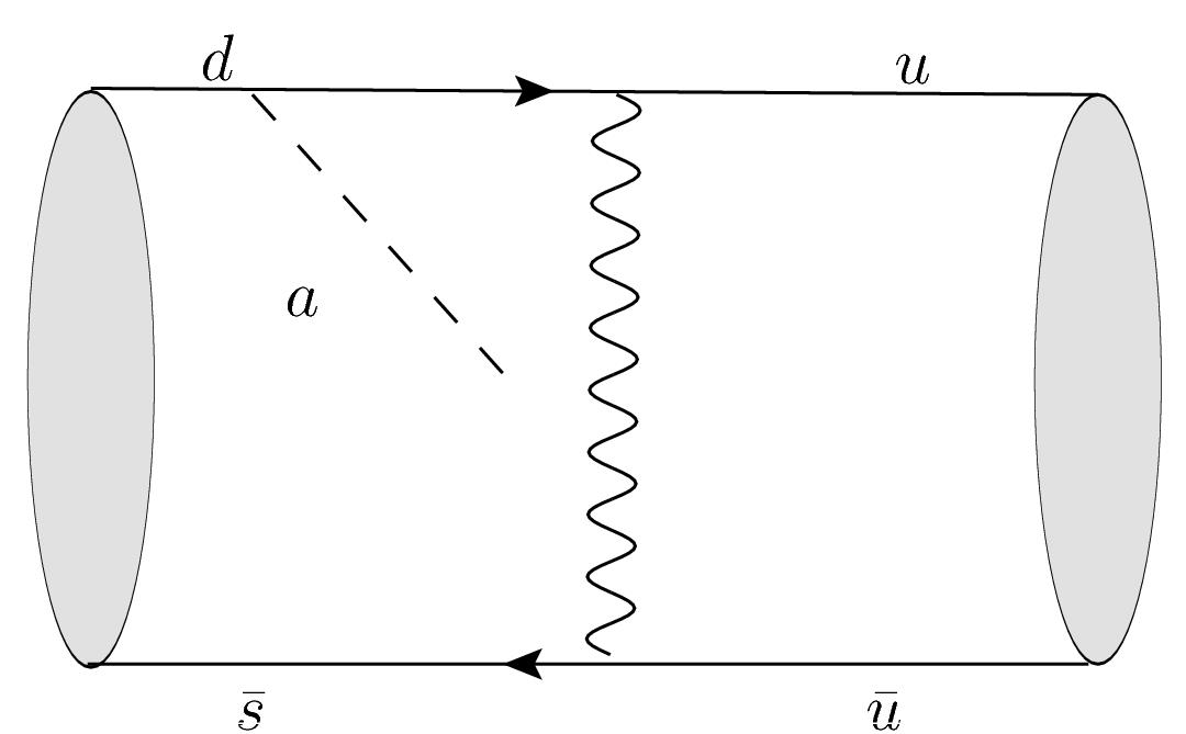
Figure 2: Tree level contribution to the amplitude for the $K^{0}\rightarrow\pi^{0}\,a$ decay, with the ALP emitted from the $K^{0}$ meson. Diagrams where the ALP is emitted from the $\pi^{0}$ quarks are straightforward. Similar diagrams can be depicted for the CP conjugate process $\bar{K}^{0}\rightarrow\pi^{0}\,a$.

Using the conventions defined in Eqs. (10) and (12), the neutral hadronic matrix element for the $K^{0}$ transition reads:

$$\bra{\pi^{0}}\,\Gamma_{1}\otimes\Gamma_{2}\ket{K^{0}}\equiv-\frac{f_{K}f_{\pi}}{\sqrt{2}}\int_{0}^{1}dx\int_{0}^{1}dy\,\mathrm{Tr}\left[\Psi_{\pi}(y)\Gamma_{(1)}\Psi_{K}(x)\Gamma_{(2)}\right]\,,$$ (18)

with the $1/\sqrt{2}$ factor taking care of the Clebsch–Gordon suppression of the decay into the neutral $\pi$ meson.

The operator insertion $\Gamma_{(1)}\otimes\Gamma_{(2)}$ is defined as $\gamma_{\mu}P_{L}\otimes\Gamma^{\mu}_{(\bar{q})}$ or $\Gamma^{\mu}_{(q)}\otimes\gamma_{\mu}P_{L}$ depending if the ALP is emitted from the $\bar{q}$ anti–quark (i.e. $\bar{s}$ for the $K^{0}$ and $\bar{u}$ for the $\pi^{0}$ meson) or from quark $q$ (i.e. the $d$ quark for the $K^{0}$ and the $u$ quark for the $\pi^{0}$ meson), respectively, with

$$\Gamma^{\mu}_{(\bar{q})} = -\frac{4G_{F}}{\sqrt{2}}V^{*}_{us}V_{ud}\left(\frac{c_{s}\,m_{s}}{f_{a}}\,\gamma_{5}\,\frac{\not{k}_{a}-\not{p}_{\bar{s}}+m_{s}}{m_{a}^{2}-2k_{a}\cdot p_{\bar{s}}}\,\gamma_{\mu}P_{L}\,-\,\frac{c_{u}\,m_{u}}{f_{a}}\,\gamma_{\mu}P_{L}\,\frac{\not{k}_{a}+\not{p}^{\prime}_{\bar{u}}-m_{u}}{m_{a}^{2}-2k_{a}\cdot p^{\prime}_{\bar{u}}}\,\gamma_{5}\right)\hskip 11.38092pt$$ (19)

$$\Gamma^{\mu}_{(q)} = -\frac{4G_{F}}{\sqrt{2}}V^{*}_{us}V_{ud}\left(\frac{c_{d}\,m_{d}}{f_{a}}\,\gamma_{\mu}P_{L}\,\frac{\not{p}_{d}-\not{k}_{a}+m_{d}}{m_{a}^{2}-2k_{a}\cdot p_{d}}\,\gamma_{5}\,+\,\frac{c_{u}\,m_{u}}{f_{a}}\,\gamma_{5}\,\frac{\not{k}_{a}+\not{p}^{\prime}_{u}+m_{u}}{m_{a}^{2}-2k_{a}\cdot p^{\prime}_{u}}\,\gamma_{\mu}P_{L}\right)$$ (20)

The $\bar{K}^{0}\to\pi^{0}\,a$ decay amplitude can be obtained similarly:

$$\bra{\pi^{0}}\,\bar{\Gamma}_{1}\otimes\bar{\Gamma}_{2}\ket{\bar{K}^{0}}\equiv-\frac{f_{K}f_{\pi}}{\sqrt{2}}\int_{0}^{1}dx\int_{0}^{1}dy\,\mathrm{Tr}\left[\Psi_{\pi}(y)\bar{\Gamma}_{(1)}\Psi_{K}(x)\bar{\Gamma}_{(2)}\right]\,,$$ (21)

with the operator insertions $\bar{\Gamma}_{(1)}\otimes\bar{\Gamma}_{(2)}$ being $\gamma_{\mu}P_{L}\otimes\bar{\Gamma}^{\mu}_{(q)}$ or $\bar{\Gamma}^{\mu}_{(\bar{q})}\otimes\gamma_{\mu}P_{L}$ with

$$\bar{\Gamma}^{\mu}_{(q)} = -\frac{4G_{F}}{\sqrt{2}}V_{us}V^{*}_{ud}\left(\frac{c_{s}\,m_{s}}{f_{a}}\,\gamma_{5}\,\frac{\not{p}_{s}-\not{k}_{a}+m_{s}}{m_{a}^{2}-2k_{a}\cdot p_{s}}\,\gamma_{\mu}P_{L}\,+\,\frac{c_{u}\,m_{u}}{f_{a}}\,\gamma_{\mu}P_{L}\,\frac{\not{k}_{a}+\not{p}^{\prime}_{u}+m_{u}}{m_{a}^{2}-2k_{a}\cdot p^{\prime}_{u}}\,\gamma_{5}\right)\hskip 14.22636pt$$ (22)

$$\bar{\Gamma}^{\mu}_{(\bar{q})} = -\frac{4G_{F}}{\sqrt{2}}V_{us}V^{*}_{ud}\left(\frac{c_{d}\,m_{d}}{f_{a}}\,\gamma_{\mu}P_{L}\,\frac{\not{k}_{a}-\not{p}_{\bar{d}}+m_{d}}{m_{a}^{2}-2k_{a}\cdot p_{\bar{d}}}\,\gamma_{5}\,-\,\frac{c_{u}\,m_{u}}{f_{a}}\,\gamma_{5}\,\frac{\not{k}_{a}+\not{p}^{\prime}_{\bar{u}}-m_{u}}{m_{a}^{2}-2k_{a}\cdot p^{\prime}_{\bar{u}}}\,\gamma_{\mu}P_{L}\right)$$ (23)

Adopting the same phase conventions as [53], one defines the neutral Kaon mass eigenstates:

$$K^{0}_{L} = \frac{1}{\sqrt{2(1+|\tilde{\epsilon}|^{2})}}\left(\left(1+\tilde{\epsilon}\right)K^{0}+\left(1-\tilde{\epsilon}\right)\bar{K}^{0}\right)$$ (24)

$$K^{0}_{S} = \frac{1}{\sqrt{2(1+|\tilde{\epsilon}|^{2})}}\left(\left(1+\tilde{\epsilon}\right)K^{0}-\left(1-\tilde{\epsilon}\right)\bar{K}^{0}\right).$$ (25)

By making the following assignments for the initial and final quark momenta,

$$p_{\bar{s}} = xP_{K}\qquad,\qquad p^{\prime}_{u}=(1-x)P_{K}$$

$$p_{d} = yP_{\pi}\qquad\,,\,\qquad p^{\prime}_{\bar{u}}=(1-y)P_{\pi}$$

the amplitude for the $K^{0}_{L}\to\pi^{0}\,a$ decay, when the ALP emitted by the $K^{0}_{L}$ meson, reads:

$$\mathcal{M}_{K^{0}_{L}} = -\frac{\tilde{\epsilon}\,G_{F}}{2\sqrt{2}}\,\real[V^{*}_{us}V_{ud}]\,f_{\bar{K}}\,f_{\pi}\,(k_{a}\cdot P_{\pi})\frac{M_{K}}{f_{a}}\,\times\,\hskip 14.22636pt$$ (26)

$$\times\int^{1}_{0}\left\{\frac{c_{s}\,m_{s}\,\theta(x-\delta^{K}_{a})}{m_{a}^{2}-2\,x\,k_{a}\cdot P_{K}}-\frac{c_{d}\,m_{d}\,\theta(1-x-\delta^{K}_{a})}{m_{a}^{2}-2\,(1-x)\,k_{a}\cdot P_{K}}\right\}\,\phi_{K}(x)\,g_{K}(x)\,dx$$

once the trivial integration in $y$ is performed. As one can notice from Eq. (26), the amplitude for the $K^{0}_{L}$ decay is proportional to the oscillation CP violation parameter $\tilde{\epsilon}$, as expected from general considerations on the CP properties of $K^{0}$ and $\bar{K}^{0}$ decays, and from the absence of imaginary part in the CKM for the tree–level diagram, i.e. $\imaginary[V^{*}_{us}V_{ud}]=0$. Consequently the $K^{0}_{L}$ decay amplitude is suppressed by $O(10^{-3})$, with respect to the corresponding tree–level charged process. Conversely, the $K^{0}_{S}\to\pi^{0}\,a$ decay amplitude can be obtained from the result of Eq. 26, simply removing the $\tilde{\epsilon}$ suppression factor, and would be of the same order as the charged process.

The amplitude contribution when the ALP is emitted from the $\pi^{0}$ meson is not explicitly reported here, showing the same $M_{\pi}/M_{K}$ suppression as for the charged decay case.

3.3 The one-loop process

Charged and neutral pseudo-scalar $K\to\pi\,a$ meson decays, assuming flavour conserving fermion-ALP interactions of Eq. (3), receive contributions at one–loop level[33, 10, 38] from the diagrams shown in Fig. 3. In the following only the contribution arising from fermion-ALP interaction will be considered.

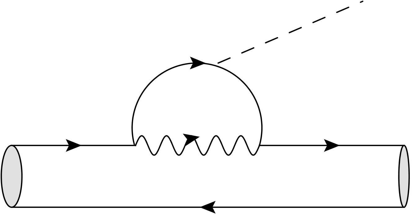
Figure 3: One-loop penguin contributions

In this kind of processes, only one quark line participate to the ALP emission, the other quark being a spectator. Customarily the hadronization of a matrix element between two pseudo-scalar meson mediated by a vector current, where one of the quark does not interact can be factorised as

$$\bra{P}\bar{q}_{1}\gamma^{\mu}Q_{2}\ket{M}=f_{+}(q^{2})(P_{M}+P_{P})^{\mu}+f_{0}(q^{2})\,q^{\mu}$$ (27)

with $q=P_{M}-P_{P}$. The form factors $f_{+,0}(0)=1$ in the isospin symmetric limit, while the non approximated, $q^{2}$ dependent, form factors are obtained from LQCD calculation [49]. From Eq. (27) the amplitude for the $K^{+}\to\pi^{+}\,a$ decay reads:

$${\mathcal{M}}^{L}_{K^{+}}=\frac{G_{F}\,m^{2}_{t}}{4\sqrt{2}\pi^{2}}(V_{ts}V_{td}^{*})\frac{M^{2}_{K^{+}}}{f_{a}}\left(1-\frac{M^{2}_{\pi^{+}}}{M^{2}_{K^{+}}}\right)\!\left[f_{+}(m_{a}^{2})+\frac{m_{a}^{2}}{M^{2}_{K^{+}}-M^{2}_{\pi^{+}}}f_{-}(m_{a}^{2})\right]\!\sum_{q=u,c,t}\!\!c^{(q)}_{sd}$$ (28)

with the coefficient

$$c^{(q)}_{sd}=\frac{V_{qi}V_{qj}^{*}}{V_{ts}V_{td}^{*}}\left[3\,c_{W}\frac{g(x_{q})}{x_{t}}-\frac{c_{q}\,x_{q}}{4\,x_{t}}\ln\left(\frac{f_{a}^{2}}{m_{q}^{2}}\right)\right]$$ (29)

opportunely normalized in order to factorize out all the relevant scale dependences. The penguin with the ALP emitted from the internal W line is included for completeness, even if in the following phenomenological analysis $c_{W}=0$ will be assumed. The dominant contribution from the penguin diagram is mostly proportional to the $c_{t}$ coupling. For the $K$ meson decay, with the charm contribution roughly accounting for $10\%$ of the total contribution.

One-loop diagrams, with the ALP emitted from the initial/final quarks can be safely neglected being suppressed by at least a factor $m_{s}^{2}/m_{W}^{2}\approx 10^{-6}$ with respect to the penguin contributions, as they arise at third order in the external momenta expansion. Therefore, no sensitivity on the ALP–down quark couplings can emerge in the $K\to\pi\,a$ decays from one loop diagrams.

An order of magnitude of the tree vs loop amplitude ratio is obtained from comparing Eqs. (16) and (28), giving:

$$R_{T/L}=\left|\frac{\mathcal{M}^{T}_{K^{+}}}{\mathcal{M}^{L}_{K^{+}}}\right|\approx 2\,\pi^{2}\frac{f_{K}\,f_{\pi}}{m_{t}^{2}}\left|\frac{V^{*}_{us}\,V_{ud}}{V^{*}_{ts}\,V_{td}}\right|\simeq 1.\times 10^{-2}\,.$$ (30)

showing the expected level of suppression. Even if the tree vs loop ratio is at the per cent level, the tree level diagrams may have a non negligible impact in the measurement of the $K\to\pi\,a$ decays, as in principle they depend on different and less constrained, down quark–ALP couplings.

Finally, the loop contribution to the $K^{0}_{L}\to\pi^{0}\,a$ decay can be easily obtained from Eq. (28) and reads:

$${\mathcal{M}}^{Loop}_{K^{0}_{L}}=\frac{G_{F}\,m^{2}_{t}}{4\,\sqrt{2}\pi^{2}}\imaginary(V_{ts}V_{td}^{*})\frac{M^{2}_{K^{+}}}{f_{a}}\left(1-\frac{M^{2}_{\pi^{+}}}{M^{2}_{K^{+}}}\right)\left[f_{+}(m_{a}^{2})+\frac{m_{a}^{2}}{M^{2}_{K^{+}}-M^{2}_{\pi^{+}}}f_{-}(m_{a}^{2})\right]\,c^{(t)}_{sd}$$

being proportional to the non vanishing imaginary part of the CKM matrix.

4 Bounds on ALP-fermion couplings

Armed with the tree–level and one–loop, charged and neutral, $K\to\pi\,a$ decays amplitudes obtained in the previous section, one can bound the ALP-fermion couplings using the experimental limits provided by the NA62 [24, 25], E949 [21, 22, 23] and KOTO [26] experiments. The main assumption underlying the following phenomenological analysis is that the ALP lifetime is sufficiently long for escaping the detector (i.e. $\tau_{a}\gtrsim 100$ ps) or alternatively the ALP is mainly decaying in a, not better specified, invisible sector. Visible ALP decays have been studied, for example, in [47, 28, 10, 38].

The tree–level amplitudes of Eqs. (3.1), (3.1) and (26) depend on the ALP couplings with $s,d$ and $u$ quarks, while the one–loop ones reported in Eqs. (28), (29) and (3.3), are typically dominated by the ALP coupling with the heaviest quark running in the loop, the $t$ quark, being the $c,u$ contributions suppressed by the $m_{u,c}/m_{t}$ mass ratio barring Cabibbo enhancements. Being the focus of this paper on ALP-fermion couplings, for the rest of the section $c_{W}=0$ will be assumed. The interplay between the simultaneous presence of $c_{W}$ and $c_{t}$ has been discussed in detail in [38].

An analysis of the $K\to\pi\,a$ decay with completely general, but flavor conserving, ALP-quark couplings, would require to consider a five-parameters fit, $(c_{u},c_{d},c_{c},c_{s},c_{t})$ beside the ALP mass $m_{a}$. In order to obtain meaningful information about the ALP-fermion couplings different simplifying assumptions have to be introduced. The phenomenological approach followed in this section will be twofold. First of all, in Sec. 4.1, all ALP-fermion couplings, introduced in the Lagrangian of Eq. (3), will be assumed independent. Then, using the tree–level amplitudes for the s– and t–channels, limits on $(c_{u},c_{s})$ and $(c_{d},c_{s})$ will be obtained respectively from the charged and neutral $K$ meson decays, setting all the other ALP-quark couplings to $0$. Afterwards, in Sec. 4.2, only two independent family universal ALP-fermion couplings, $c_{\uparrow}$ for the up quarks and $c_{\downarrow}$ for the down ones, will considered, for sake of simplicity. Under this assumption, the interplay between the tree–level and loop contributions to the $K\to\pi\,a$ decay will be thoroughly discussed. Limits for the universal ALP–fermion coupling $c_{a\Phi}$ can be then obtained straightforwardly.

4.1 Tree–level Contributions

The tree–level amplitudes for charged and neutral $K$ decays, given by Eq. (3.1) and (26) for charged and neutral channels respectively, in the most general case depend on four parameters: the ALP couplings to the three light quarks, $c_{u},c_{d}$ and $c_{s}$ and the ALP mass, $m_{a}$. As derived in Eq. (3.1) the diagram with the ALP emitted by the pion contribution is strongly suppressed, ranging from $10^{-2}$ (in the most conservative case) to $0$ if $g_{\pi}=0$ is assumed. Therefore, it seems reasonable, in the following, to neglect the $\pi$-ALP emission diagrams, and, consequently the $K^{+}$ decay rate depends only on the $(c_{u},c_{s})$ ALP-fermion couplings, while the $K^{0}$ decay rates only on $(c_{d},c_{s})$ ones.

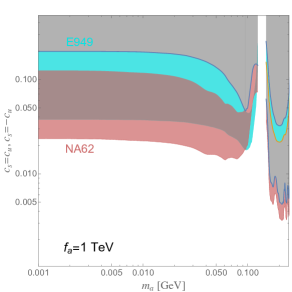
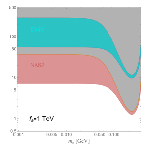
Figure 4: Excluded parameter regions derived from tree-level channels for charged (left) and neutral (right) $K\to\pi a$ decays. In the left–plot limits are derived from NA62 (pink) and E949 (cyan) experiments. In the right–plot, bounds are obtained from present (cyan) and expected (pink) KOTO data.

The left plot in Fig. 4 shows the allowed regions of parameters as function of the ALP mass $m_{a}$ for the chosen reference value $f_{a}=1$ TeV. The shaded gray area is excluded by present experimental data. The upper and lower contours, delimiting the colored shaded area represent the bounds obtained setting $c_{s}=c_{u}$ and $c_{s}=-c_{u}$ respectively. The exclusive limit on $c_{s}\,(c_{u})$ with $c_{u}\,(c_{s})=0$ lies inside the colored shaded area. As noticed in Sec. 3, for $c_{s}=c_{u}$ the $K^{+}$ decay rate gets suppressed by an accidental parametric cancellation, leading to a less stringent bound on the ALP–fermion couplings. The shaded colored area represent consequently the typical uncertainty in the bound prediction from $K^{+}\to\pi^{+}\,a$ decay rates once letting the couplings $(c_{u},c_{s})$ freely varying in the $|c_{s}/c_{u}|\leq 1$ range. The pink contours and shaded region are obtained from NA62 data [24, 25] while the cyan ones refer to bounds obtained from the E949 [21] experiment. For $m_{a}$ values below $0.15$ GeV the two experiments provide similar results, with a slight edge in favor of NA62, bounding $(c_{u},c_{s})\lesssim 0.05$. In the $m_{a}>0.15$ region, latest NA62 measurements has instead improved the sensitivity of E949 by roughly a factor 10, bounding $(c_{u},c_{s})\lesssim 0.01$. For $m_{a}\approx m_{\pi^{0}}$ both experiments loose sensitivity. No significative effects are obtained in this plot from the $\pi$-ALP emission diagrams, once the $c_{d}$ parameter is assumed to lie in the perturbative range.

A similar analysis, for $K^{0}_{L}\to\pi^{0}\,a$ decay is presented in the right plot of Fig. 4, where the cyan and pink regions are obtained using the present[26] and expected KOTO experiment data, respectively. For this plot the upper and lower contours, delimiting the shaded area represent the bounds obtained setting on $c_{s}=c_{d}$ and $c_{s}=-c_{d}$ respectively. KOTO experiment results much less sensitive to the $(c_{d},c_{s})$ ALP-fermion couplings, as CP violation in the tree–level processes can occurs only through the CP-mixing $\tilde{\epsilon}$ parameter, thus suppressing this channel by roughly a factor $10^{-3}$. Present KOTO data do not provide any real constraint, with the prospect that future data could reach sensitivity to the perturbativity region.

The results showed in Fig. 4, even if not looking flashy, represent, nonetheless, the most stringent model–independent bounds on light quark couplings to ALP, for an ALP mass in the sub–GeV range, once flavour conserving, but not flavor universal ALP-fermion interactions, are assumed.

4.2 Interplay between tree–level and one–loop contributions

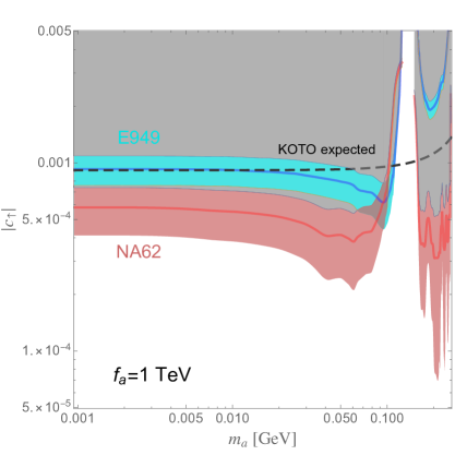
Figure 5: Excluded parameter regions for an universal ALP–up quark coupling $c_{\uparrow}$ derived from NA62 (pink), E949 (cyan) and KOTO expected (dashed line) experiments.

To constrain, simultaneously, tree–level and one–loop contributions to the $K\to\pi\,a$ decay one has to adopt simplified frameworks. Following [38], one can consider the scenario of universal ALP-quark coupling, $c_{a\Phi}$. From the analysis of Sec. 3 one easily realizes that in this scenario, the top-penguin loop contribution dominates the charged and neutral $K$ decay, once $c_{W}=0$ is assumed. The full cyan and pink lines in Fig. 5, represent the limits on $c_{a\Phi}$ obtained from E949 and NA62 respectively as function of the ALP mass $m_{a}$. The dashed gray line represents, instead, the $c_{a\Phi}$ limits from the expected KOTO upgrade. These results are in agreement with the bounds presented in [38] and show that $K$ meson decays typically constrain $c_{a\Phi}\lesssim 10^{-3}$ in the sub-GeV ALP mass range.

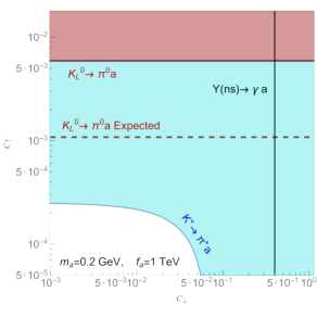
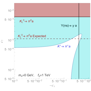
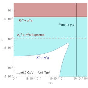
Figure 6: Excluded parameter regions for universal ALP–up and down quark couplings $c_{\uparrow}$ and $c_{\downarrow}$ derived from NA62 (cyan) and KOTO (pink and dashed pink line) and $Y(ns)\to\gamma\,a$ (full vertical black line) experiments. The upper plots refer to the $\rm{sign}(c_{\downarrow})=\rm{sign}(c_{\uparrow})$ case, while in the lower ones $\rm{sign}(c_{\downarrow})=-\rm{sign}(c_{\uparrow})$ has been chosen.

In general MFV ALP frameworks, however, it may not be unconceivable to assign different, but flavor universal, PQ charges to the up and down quark sectors, see for example [54, 44, 45], that in the following will be denoted as $c_{\uparrow}$ and $c_{\downarrow}$, respectively. In this scenario, one–loop amplitudes only depend from $c_{\uparrow}$ while the tree–level amplitudes are practically proportional to a linear combination of $c_{\uparrow}$ and $c_{\downarrow}$, as evident for example in the simplified amplitudes of Eqs. (16) and (17). From the tree–level analysis, summarized in Fig. 4, one learns that present data limit $c_{\downarrow}$ to be typically below $10^{-1}$. Indeed, to study the interplay between tree–level and one–loop the reference value $c_{\downarrow}=\pm 0.05$ has been chosen, somehow in the ridge of the parameters allowed from the previous analysis on tree–level contributions. The blue and brown shaded regions showed in Fig. 5 represent the variability of NA62 and E979 bounds on $c_{\uparrow}$ once $c_{\downarrow}$ is let varying in the $[-0.05,0.05]$ range. The presence of the tree-level contribution can modify the bounds on $c_{\uparrow}$ extracted from penguin diagrams of roughly one order of magnitude, in all the $m_{a}$ range. The expected KOTO limits on the $K^{0}_{L}\to\pi^{0}\,a$ decay is reported in Fig. 5 as a black dashed line, giving a practically constant bound $c_{\uparrow}\lesssim 1\times 10^{-3}$ over all the $m_{a}$ range of interest, yet not competitive with the charged sector one. Notice that, however, the neutral $K$ decay sector does not suffer from any relevant interference from the tree–level processes, largely suppressed from the CP violating parameter $\tilde{\epsilon}$. A simultaneous measurement of the charged and neutral $K\to\pi\,a$ decays, may thus in a not too far future may give independent indications on the relative size of the ALP–light quark couplings.

Finally, in Fig. 6, a summary on the combined bounds on $(c_{\uparrow},c_{\downarrow})$ is presented for two reference values of the ALP mass $m_{a}=0$ GeV and $m_{a}=0.2$ GeV. For the two upper plots $\rm{sign}(c_{\downarrow})=\rm{sign}(c_{\uparrow})$ has been taken. In the lower plots, where $\rm{sign}(c_{\downarrow})=-\rm{sign}(c_{\uparrow})$ has been considered, a partial cancellation between one–loop and tree-level contributions takes place. In this second scenario, the $c_{\downarrow}$ constraint from the $\Upsilon(ns)$ decays at Babar and Belle (full vertical black line) derived by [55] can contribute to close this flat direction.

5 Conclusions

In this letter, a detailed analysis of the $K\to\pi a$ decay has been presented, in view of the recent NA62 measurement and the foreseen updates from the KOTO experiment. Assuming flavor and CP conserving ALP couplings with fermions, the dominant contribution to the $K\to\pi a$ decays arises from the penguin diagrams, manly proportional to the $c_{t}$ coupling. NA62 and E949 experiments bound $c_{t}$ to be smaller than $6\times 10^{-4}$ in most of the allowed $m_{a}$ region, for the chosen reference value of the PQ symmetry breaking scale $f_{a}=1$ TeV. Expected KOTO results can provide comparable bounds on the $c_{t}$ coupling. Subdominant tree–level diagrams can, however, contribute to the $K\to\pi a$ decay process. The tree-level amplitudes contributing to the $K^{+}\to\pi^{+}a$ and $K^{0}_{L}\to\pi^{0}a$ decays have been derived in this letter, following the Lepage–Brodsky [39, 40] technique. Assuming all ALP couplings with fermions to be vanishing, but $(c_{u},c_{s})$, independent limits on the the light quark–ALP couplings $(c_{u},c_{s})\sim 0.05$ can be obtained in the allowed $m_{a}$ mass range, from NA62 and E949 experiments. KOTO experiment, conversely, will not provide competitive bounds on the $(c_{d},c_{s})$ couplings, due to the SM CP violating suppression of the $K^{0}_{L}$ channel.

If a universal ALP coupling to fermions, $c_{a\Phi}$, is assumed, the results presented in this letter confirm and refine previous analysis [33, 34, 38], where only penguin contributions were considered. However, in general MFV ALP frameworks it may not be unconceivable to assign different, but flavor universal, PQ charges to the up and down quark sectors. In this case the simpler ”penguin dominated” result may be significantly modified. The subdominant tree-level contribution proportional to $c_{\downarrow}$ can strongly interfere with the measurement of $c_{\uparrow}$, introducing an uncertainty band of roughly one order of magnitude. Similar analysis should be extended to all meson decays in ALP[48].

6 Acknowledgements

The authors thank O. Sumensari for useful discussions in the early stage of this paper. A.G. and S.R. acknowledge support from the European Union’s Horizon 2020 research and innovation programme under the Marie Sklodowska-Curiegrant agreements 690575 (RISE InvisiblesPlus) and 674896 (ITN ELUSIVES). This project has received funding/support from the European Union’s Horizon 2020 research and innovation programme under the Marie Sklodowska-Curie grant agreement No 860881-HIDDEN.

References

- [1] R.D. Peccei and Helen R. Quinn. CP Conservation in the Presence of Instantons. Phys. Rev. Lett., 38:1440–1443, 1977.
- [2] F. Wilczek. Problem of strong and invariance in the presence of instantons. Phys. Rev. Lett., 40:279–282, Jan 1978.
- [3] Steven Weinberg. A new light boson? Phys. Rev. Lett., 40:223–226, Jan 1978.
- [4] Jihn E. Kim. Weak-interaction singlet and strong invariance. Phys. Rev. Lett., 43:103–107, Jul 1979.
- [5] M.A. Shifman, A.I. Vainshtein, and V.I. Zakharov. Can confinement ensure natural cp invariance of strong interactions? Nuclear Physics B, 166(3):493 – 506, 1980.
- [6] A.R. Zhitnitsky. On Possible Suppression of the Axion Hadron Interactions. (In Russian). Sov. J. Nucl. Phys., 31:260, 1980.
- [7] Michael Dine, Willy Fischler, and Mark Srednicki. A simple solution to the strong cp problem with a harmless axion. Physics Letters B, 104(3):199 – 202, 1981.
- [8] Ken Mimasu and Verónica Sanz. ALPs at Colliders. JHEP, 06:173, 2015.
- [9] Joerg Jaeckel and Michael Spannowsky. Probing MeV to 90 GeV axion-like particles with LEP and LHC. Phys. Lett. B, 753:482–487, 2016.
- [10] Martin Bauer, Matthias Neubert, and Andrea Thamm. Collider Probes of Axion-Like Particles. JHEP, 12:044, 2017.
- [11] I. Brivio, M.B. Gavela, L. Merlo, K. Mimasu, J.M. No, R. del Rey, and V. Sanz. ALPs Effective Field Theory and Collider Signatures. Eur. Phys. J. C, 77(8):572, 2017.
- [12] G. Alonso-Álvarez, M.B. Gavela, and P. Quilez. Axion couplings to electroweak gauge bosons. Eur. Phys. J. C, 79(3):223, 2019.
- [13] Lucian Harland-Lang, Joerg Jaeckel, and Michael Spannowsky. A fresh look at ALP searches in fixed target experiments. Phys. Lett. B, 793:281–289, 2019.
- [14] Cristian Baldenegro, Sylvain Fichet, Gero von Gersdorff, and Christophe Royon. Searching for axion-like particles with proton tagging at the LHC. JHEP, 06:131, 2018.
- [15] Jorge Martin Camalich, Maxim Pospelov, Pham Ngoc Hoa Vuong, Robert Ziegler, and Jure Zupan. Quark Flavor Phenomenology of the QCD Axion. Phys. Rev. D, 102(1):015023, 2020.
- [16] Davide Cadamuro and Javier Redondo. Cosmological bounds on pseudo Nambu-Goldstone bosons. JCAP, 02:032, 2012.
- [17] Marius Millea, Lloyd Knox, and Brian Fields. New Bounds for Axions and Axion-Like Particles with keV-GeV Masses. Phys. Rev. D, 92(2):023010, 2015.
- [18] Luca Di Luzio, Federico Mescia, and Enrico Nardi. Redefining the Axion Window. Phys. Rev. Lett., 118(3):031801, 2017.
- [19] Igor G. Irastorza and Javier Redondo. New experimental approaches in the search for axion-like particles. Prog. Part. Nucl. Phys., 102:89–159, 2018.
- [20] Rouven Essig et al. Working Group Report: New Light Weakly Coupled Particles. In Community Summer Study 2013: Snowmass on the Mississippi, 10 2013.
- [21] A. V. Artamonov et al. Study of the decay in the momentum region MeV/c. Phys. Rev. D, 79:092004, 2009.
- [22] A.V. Artamonov et al. New measurement of the branching ratio. Phys. Rev. Lett., 101:191802, 2008.
- [23] S. Adler et al. Measurement of the K+ – pi+ nu nu branching ratio. Phys. Rev. D, 77:052003, 2008.
- [24] Eduardo Cortina Gil et al. Search for a feebly interacting particle in the decay . JHEP, 03:058, 2021.
- [25] Eduardo Cortina Gil et al. Measurement of the very rare decay. arXiv 2103.15389.
- [26] J.K. Ahn et al. Search for the and decays at the J-PARC KOTO experiment. Phys. Rev. Lett., 122(2):021802, 2019.
- [27] Sergey Alekhin et al. A facility to Search for Hidden Particles at the CERN SPS: the SHiP physics case. Rept. Prog. Phys., 79(12):124201, 2016.
- [28] Kevin J. Kelly, Soubhik Kumar, and Zhen Liu. Heavy Axion Opportunities at the DUNE Near Detector. 11 2020.
- [29] Roel Aaij et al. Search for hidden-sector bosons in decays. Phys. Rev. Lett., 115(16):161802, 2015.
- [30] R. Aaij et al. Search for long-lived scalar particles in decays. Phys. Rev. D, 95(7):071101, 2017.
- [31] Eduard Masso and Ramon Toldra. On a light spinless particle coupled to photons. Phys. Rev. D, 52:1755–1763, 1995.
- [32] A.J. Bevan et al. The Physics of the B Factories. Eur. Phys. J. C, 74:3026, 2014.
- [33] Eder Izaguirre, Tongyan Lin, and Brian Shuve. Searching for Axionlike Particles in Flavor-Changing Neutral Current Processes. Phys. Rev. Lett., 118(11):111802, 2017.
- [34] Matthew J. Dolan, Torben Ferber, Christopher Hearty, Felix Kahlhoefer, and Kai Schmidt-Hoberg. Revised constraints and Belle II sensitivity for visible and invisible axion-like particles. JHEP, 12:094, 2017.
- [35] W. Altmannshofer et al. The Belle II Physics Book. PTEP, 2019(12):123C01, 2019. [Erratum: PTEP 2020, 029201 (2020)].
- [36] Xabier Cid Vidal, Alberto Mariotti, Diego Redigolo, Filippo Sala, and Kohsaku Tobioka. New Axion Searches at Flavor Factories. JHEP, 01:113, 2019. [Erratum: JHEP 06, 141 (2020)].
- [37] Patrick deNiverville, Hye-Sung Lee, and Min-Seok Seo. Implications of the dark axion portal for the muon g-2, B-factories, fixed target neutrino experiments and beam dumps. Phys. Rev. D, 98(11):115011, 2018.
- [38] M.B. Gavela, R. Houtz, P. Quilez, R. Del Rey, and O. Sumensari. Flavor constraints on electroweak ALP couplings. Eur. Phys. J. C, 79(5):369, 2019.
- [39] G.Peter Lepage and Stanley J. Brodsky. Exclusive Processes in Perturbative Quantum Chromodynamics. Phys. Rev. D, 22:2157, 1980.
- [40] Adam Szczepaniak, Ernest M. Henley, and Stanley J. Brodsky. Perturbative {QCD} Effects in Heavy Meson Decays. Phys. Lett. B, 243:287–292, 1990.
- [41] Howard Georgi, David B. Kaplan, and Lisa Randall. Manifesting the Invisible Axion at Low-energies. Phys. Lett. B, 169:73–78, 1986.
- [42] Martin Bauer, Matthias Neubert, Sophie Renner, Marvin Schnubel, and Andrea Thamm. Consistent treatment of axions in the weak chiral Lagrangian. arXiv 2102.13112.
- [43] I. Brivio, M. B. Gavela, S. Pascoli, R. del Rey, and S. Saa. The Axion and the Goldstone Higgs. Chin. J. Phys., 61:55–71, 2019.
- [44] L. Merlo, F. Pobbe, and S. Rigolin. The Minimal Axion Minimal Linear Model. Eur. Phys. J. C, 78(5):415, 2018. [Erratum: Eur.Phys.J.C 79, 963 (2019)].
- [45] Javier Alonso-González, Luca Merlo, Federico Pobbe, Stefano Rigolin, and Olcyr Sumensari. Testable axion-like particles in the minimal linear model. Nucl. Phys. B, 950:114839, 2020.
- [46] Howard Georgi and Lisa Randall. Flavor Conserving CP Violation in Invisible Axion Models. Nucl. Phys. B, 276:241–252, 1986.
- [47] Luca Di Luzio, Ramona Gröber, and Paride Paradisi. Hunting for the CP violating ALP. 10 2020.
- [48] A. Guerrera and S. Rigolin. Work in preparation.
- [49] N. Carrasco, P. Lami, V. Lubicz, L. Riggio, S. Simula, and C. Tarantino. semileptonic form factors with twisted mass fermions. Phys. Rev. D, 93(11):114512, 2016.
- [50] Y.G. Aditya, Kristopher J. Healey, and Alexey A. Petrov. Searching for super-WIMPs in leptonic heavy meson decays. Phys. Lett. B, 710:118–124, 2012.
- [51] Derek E. Hazard and Alexey A. Petrov. Lepton flavor violating quarkonium decays. Phys. Rev. D, 94(7):074023, 2016.
- [52] Bhubanjyoti Bhattacharya, Cody M. Grant, and Alexey A. Petrov. Invisible widths of heavy mesons. Phys. Rev. D, 99(9):093010, 2019.
- [53] Andrzej J. Buras. Weak Hamiltonian, CP violation and rare decays. hep-ph/9806471.
- [54] F. Arias-Aragon and L. Merlo. The Minimal Flavour Violating Axion. JHEP, 10:168, 2017. [Erratum: JHEP 11, 152 (2019)].
- [55] L. Merlo, F. Pobbe, S. Rigolin, and O. Sumensari. Revisiting the production of ALPs at B-factories. JHEP, 06:091, 2019.