Unsupervised Co-part Segmentation through Assembly

Abstract

Co-part segmentation is an important problem in computer vision for its rich applications. We propose an unsupervised learning approach for co-part segmentation from images. For the training stage, we leverage motion information embedded in videos and explicitly extract latent representations to segment meaningful object parts. More importantly, we introduce a dual procedure of part-assembly to form a closed loop with part-segmentation, enabling an effective self-supervision. We demonstrate the effectiveness of our approach with a host of extensive experiments, ranging from human bodies, hands, quadruped, and robot arms. We show that our approach can achieve meaningful and compact part segmentation, outperforming state-of-the-art approaches on diverse benchmarks.

1 Introduction

Part-structure provides a compact and meaningful intermediate shape representation of articulated objects. Co-part segmentation, which aims to label semantic part belonging for each pixel of the objects in an image, is an important problem in computer vision. Such capability can directly serve various higher-level tasks such as marker-less motion tracking, action recognition and prediction, robot manipulation, and human-machine interaction.

With the advent of deep learning, and the availability of large amount of annotated motion datasets, supervised learning-based approaches have led to superior performances over traditional part segmentation methods; the most success has been achieved for human pose estimation, e.g.,  (Güler et al., 2018; Kanazawa et al., 2018). However, this approach assumes significant domain knowledge, and highly depends on the specific dataset used for training, thus making it difficult to generalize to objects with different appearance, lighting or pose, not to mention unseen subjects.

A video sequence is viewed as a spatio-temporal intensity volume that contains all structural and motion information of the action, including poses of the subject at any time as well as the dynamic transitions between the poses. Our goal in this research is to extract a general part-based representation from videos. Compared with single image-based segmentation, our work intends to aggregate shape correlation information from multiple images to improve the segmentation of individual images. The capability of consistently detecting object parts are important for motion tracking of creatures of various topology, and ultimately extracting their skeletal structures.

A successful line of recent works in this direction formulates the task as an image generation problem, where segmented parts are globally warped to form the final image. There, part-segmentation becomes the essential intermediate step, because: the better you can segment (parts), the better you can generate (the image). In this paper, we follow the same image-generation concept, but introduce a dual procedure of part-assembly to form a closed loop with part-segmentation, which ensures more consistent, also more compact and meaningful part segmentation. Specifically, we generate the final image through blending each part’s warped image, instead of a global image warping. In essence, our image based assembly operation effectively constrains the manifold of each individual part, resulting in improved results.

We take an unsupervised learning approach. Like many recent works about unsupervised / self-supervised part segmentation, we believe shape correlation information between different frames can be leveraged for achieving semantic consistency. Our approach is similar to PSD (Xu et al., 2019), Motion Co-part (Lathuilière et al., 2020) and Flow Capsule (Sabour et al., 2020), in the use of motion cues embedded in different frames for co-part segmentation. We go beyond the existing techniques in multiple ways:

1. In our method, the supervision is attained by introducing a novel dual-procedure of part-assembly to form a close loop with part-segmentation.

2. The learned parts and their transformation have clear explainable physical meaning.

3. Our method doesn’t require any field-based global warping operation, which enables handling dramatically dynamic motions.

We demonstrate the advantages of our method both visually and quantitatively. Extensive experiments have been conducted on datasets showcasing challenges due to the change in appearance, occlusions, scale and background. We also compared with recent works including NEM (Greff et al., 2017), R-NEM (Steenkiste et al., 2018), PSD (Xu et al., 2019), SCOPS (Hung et al., 2019), Motion Co-part (Lathuilière et al., 2020) and Flow Capsule (Sabour et al., 2020). Our method outperforms state-of-the-art methods in quantitative evaluation.

2 Related work

Part-based Representation

In analyzing images, describing object as a collection of parts, each with a range of possible states, is a classical framework for learning an object representation in computer vision  (Ross & Zemel, 2006; Nguyen et al., 2013). The states can be computed based on different evidences, such as visual and semantic features (Wang & Yuille, 2015), geometric shape and its behavior under viewpoint changes (Eslami & Williams, 2012) and object articulation (Sun & Savarese, 2011), resulting in a large variation of part partition. Our work performs motion-based part segmentation, where each part is constituted with a group of pixels moving together.

Motion-based Co-part Segmentation

Motion-based Co-part segmentation has been an important problem in understanding and reconstructing dynamic scenes. Articulated object can be naturally segmented as a group of rigid parts, if prior knowledge on underlying kinematic structure is known. However, this assumption does not hold in our problem setting. Most of the traditional computer vision technology recovers rigid part and kinematic structure by exploiting motion information, in particular, RGB image sequences with feature points tracked over time. There have been three main approaches: (i) motion segmentation and factorization (Yan & Pollefeys, 2008), (ii) probabilistic graphical model (Ross et al., 2010; Sturm et al., 2011), and (iii) cost function based optimization methods (Ochs et al., 2014; Keuper et al., 2015). The work from Chang and Demiris (Chang & Demiris, 2018) achieved state-of-the-art performance on the reconstruction of articulated structures from 2D image sequences. There, the segmentation was executed on tracked key-points, rather than all pixels like in our approach; the method, however, is prone to image noise, occlusions, deformations and cannot deal with articulated structures of high complexity.

Unsupervised Co-part Segmentation

With the popularity of deep neural networks, motion part segmentation has achieved superior performance in domains where labeled data are abundant, such as faces (Khan et al., 2015) and human bodies (Güler et al., 2018; Kanazawa et al., 2018). Parts segmentation can also be learned in an entirely unsupervised fashion. Nonnegative Matrix Factorization (NMF)  (Lee & Seung, 1999) learned features that exhibit sparse part-based representation of data to disentangle the hidden structure of data. (Collins et al., 2018) further proposed deep feature factorization (DFF) to estimate the common part segments in images through NMF. Leveraging on semantic consistency in an image collection of single object category, Hung et. al. (Hung et al., 2019) proposed a self-supervised network SCOPS to predict part segmentation based on the pre-trained CNN features. (Xu et al., 2019) proposed a deep model to discover object parts and the associated hierarchical structure and dynamical model from unlabeled videos. However, they assume that pre-computed motion information is available. (Lathuilière et al., 2020) proposed a model to leverage motion information with the purpose of obtaining segments that correspond to group of pixels associated to object parts moving together. But the transformation between parts in different frame is not explainable, and the motion merge to flow rather than on each part. (Sabour et al., 2020) proposed exploit motion as a powerful perceptual cue for part definition, using an expressive decoder for part generation and layered image formation with occlusion. But they still rely on flow to warp image, instead of considering that each part has independent motion.

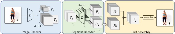
Figure 1: Architecture. Our segmentation network consists of three major components. Left: The Image Encoder takes an image $I$ as input and outputs latent feature maps $\{V_{k}\}$ and part transformations $\{T_{k}\}$ of every part. Middle: The Segment Decoder converts each feature map $V_{k}$ into a part image $P_{k}$ and a corresponding depth map $D_{k}$. Right: During the Part Assembly procedure, the depth maps $\{D_{k}\}$ are converted into part masks $\{M_{k}\}$. The masked part images $\{\tilde{I}_{k}\}$ are then assembled to generate a reconstructed image $\tilde{I}$.

3 Method

Our goal is to train a deep neural network to compute part segmentations and estimate part motions from a single input image. We train our network using an image collection of the same object category, which can be extracted from videos of an animating object. Our unsupervised training process guides the network to identify object parts in the images by observing their motions. To facilitate the training, we assemble the generated parts to recover the input images, which can be considered a dual-procedure of part segmentation. In what follows, we will first introduce our segmentation model in detail, then discuss the objectives and the training process.

3.1 Model

Our part segmentation network consists of an image encoder network and a segment decoder network. The image encoder encodes a given image into a set of latent feature maps, each corresponding to an object part. The segment decoder then decodes these part feature maps into part segments, which are later assembled to reconstruct the input image. Figure 1 provides an overview of the proposed network structure.

Image Encoder

Given an image $I\in\mathbf{R}^{H\times{}W\times{}C}$ as input, the image encoder, $\mathcal{E}$, computes latent representations of $K$ part segments, each represented by a feature map, $V_{k}\in{}\mathbf{R}^{H^{\prime}\times{}W^{\prime}\times{}C^{\prime}}$, where $k\in\mathcal{K}$ and $\mathcal{K}=\{1,\dots,K\}$ is the set of part indices. These latent feature maps implicitly capture the shapes, appearances, locations, and poses of the corresponding part segments in the input image. We treat the background region as a special part segment and represent the corresponding feature map as $V_{0}$.

The encoder also estimates a set of affine transformations, $\{T_{k}\}$, for each part $k\in\mathcal{K}$. We assume there exists a set of canonical parts located at the center of the image, which are shared by all the images and can be transformed by $\{T_{k}\}$ to match the current parts in the input image. We use $V_{k}^{*}$ to represent the feature map of a canonical part.

In our implementation, a transformation, $T$, is given by a 6-tuple

$$T=(s_{x},s_{y},s_{\theta},c_{\theta},t_{x},t_{y})$$ (1)

where $(s_{x},s_{y})$ and $(t_{x},t_{y})$ represent the scaling and the translation of the transformation. To avoid the continuity issue of angle representations (Zhou et al., 2019), we use two variables $(s_{\theta},c_{\theta})$ to represent a rotation $\theta$, which correspond to the sine and cosine of $\theta$ respectively. The transformation matrix of $T$ is then given by

$$T=\left[\begin{array}[]{cc}A&\bm{t}\\ \bm{0}&1\end{array}\right]$$ (2)

where

$$A=\left[\begin{array}[]{cc}\bar{c}_{\theta}&-\bar{s}_{\theta}\\ \bar{s}_{\theta}&\bar{c}_{\theta}\end{array}\right]\left[\begin{array}[]{cc}s_{x}&0\\ 0&s_{y}\end{array}\right],\bm{t}=\left[\begin{array}[]{c}t_{x}\\ t_{y}\end{array}\right]$$

and $(\bar{s}_{\theta},\bar{c}_{\theta})=(s_{\theta},c_{\theta})/\parallel(s_{\theta},c_{\theta})\parallel_{2}$.

Segment Decoder

The segment decoder network, $\mathcal{D}$, is trained to convert a latent feature map ${V_{k}}$ into a part image, $P_{k}\in{}\mathbf{R}^{H\times{}W\times{}C}$, which recovers the appearance of the part in the original image.

We use the same decoder network $\mathcal{D}$ to convert feature maps of all the object parts and the background into part images. The decoder $\mathcal{D}$ also outputs a depth map, $D_{k}\in{}\mathbf{R}^{H\times{}W}$, for each part. With $\bm{u}$ representing the coordinates of a pixel, $D_{k}(\bm{u})$ is a scalar that specifies the relative inverse depth of the corresponding pixel located at $\bm{u}$ in part image $P_{k}$. We assume that the object is composed of opaque parts, so that a part with smaller inverse depth (thus farther from the camera) will be partially occlude by the parts with larger inverse depth. The part mask $M_{k}\in\bm{R}^{H\times{}W}$ is thus a pixel-wise visibility mask indicating whether a pixel in the part image $P_{k}$ is visible in the original image, which can be computed as

$$M_{k}(\bm{u})=\operatorname*{softmax}\limits_{l\in{}\{0\}\cup{}\mathcal{K}}D_{l}(\bm{u})$$ (3)

Part Assembly

We train the segmentation network by assembling the part images together and reconstructing the input image. This is achieved by gathering the visible pixels from all the part images. Specifically, the reconstructed image $\tilde{I}$ is computed as $\tilde{I}=\sum_{k=0}^{K}\tilde{I}_{k}$ where $\tilde{I}_{k}$ is the visible part of part image $P_{k}$ as specified by the part mask $M_{k}$. We compute $\tilde{I}_{k}$ using $\tilde{I}_{k}={M}_{k}\odot{}P_{k}$, where $\odot$ is the Hadamard (pixel-wise) product between two arrays.

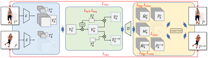
Figure 2: Training Process. We train our segmentation network in an end-to-end fashion. Left: The encoder $\mathcal{E}$ converts both the source image $I^{s}$ and the target image $I^{t}$ into latent feature maps and estimates part transformations. Middle: The source latent feature maps $V_{k}^{s}$ is inversely transformed into the canonical feature map $V_{k}^{*}$ using the source transformation $T_{k}^{s}$. $V_{k}^{*}$ is then transformed using $T_{k}^{s}$ and the target transformation $T_{k}^{t}$, producing a recovered feature map $\tilde{V}_{k}^{s}$ and a retargeted feature map $\tilde{V}_{k}^{s\rightarrow{}t}$ respectively. Right: The decoder $\mathcal{D}$ assembles the resulting $\{\tilde{V}_{k}^{s}\}$ and $\{\tilde{V}_{k}^{s\rightarrow{}t}\}$ and generates a reconstructed source image $\tilde{I}^{s}$ and a retargeted image $\tilde{I}^{s\rightarrow{}t}$ respectively. Those generated images are then compared with the input to compute losses.

3.2 Training

We train our co-part segmentation network using image pairs randomly selected from the input image collection. During training, we require the network to reconstruct one image of a pair (the source image, $I^{s}$) as accurate as possible, while using the other image of the pair (the target image, $I^{t}$) to cross-validate the latent representation of the parts and the segmentation results. This validation is performed by constructing the target image using the part segments extracted from the source image. Unlike the existing works that warp the source image using optical flow (Siarohin et al., 2019, 2020; Sabour et al., 2020), we transform the parts in latent space directly and decode the transformed latent features of the parts to generate the target image.

Figure 2 provides an overview of this training process. In more details, the encoder network $\mathcal{E}$ takes the two images $I^{s}$ and $I^{t}$ as input and computes latent feature maps and part transformations for both of them. The results are denoted as $\{V^{s}_{0},(V_{k}^{s},T_{k}^{s})\}$ and $\{V^{t}_{0},(V_{k}^{t},T_{k}^{t})\}$ respectively. We transform each source latent feature map $V_{k}^{s}$ using the corresponding transformations $T_{k}^{s}$ and $T_{k}^{t}$, and assemble the resulting latent maps $\{\tilde{V}^{s\rightarrow{}t}_{0},\tilde{V}^{s\rightarrow{}t}_{k}\}$ using the segment decoder $\mathcal{D}$ to produce the retargeted image $\tilde{I}^{s\rightarrow{}t}$. Note that we assume the background is static and use $\tilde{V}^{s\rightarrow{}t}_{0}=V^{s}_{0}$ in this transformation.

This retargeting is performed in two steps. First, we inversely transform $V_{k}^{s}$ using $T_{k}^{s}$ to compute the canonical latent feature map $V_{k}^{*}=({T_{k}^{s}})^{-1}\circ{}V_{k}^{s}$, which is assumed to be shared by both the source and the target. The transformation operation $\circ{}$ is defined as

$$(T\circ{}V)(\bm{u})=V(T^{-1}\bm{u})$$ (4)

where $\bm{u}$ and its transformed counterpart $T^{-1}\bm{u}$ are both coordinates of pixels. Then the target transformation $T_{k}^{t}$ is applied to $V_{k}^{*}$ to compute the retargeted feature map $\tilde{V}^{s\rightarrow{}t}_{k}={T_{k}^{t}}\circ{}{V_{k}^{*}}=[{T_{k}^{t}}(T_{k}^{s})^{-1}]\circ{}{V_{k}^{*}}$. We also recover the source feature map from $V_{k}^{*}$ as $\tilde{V}^{s}_{k}={T_{k}^{s}}\circ{}{V_{k}^{*}}$. We find this additional procedure helpful in facilitating the training at the early stage of the process.

The resulting feature maps $\{\tilde{V}^{s}_{0},\tilde{V}^{s}_{k}\}$ and $\{\tilde{V}^{s\rightarrow{}t}_{0},\tilde{V}^{s\rightarrow{}t}_{k}\}$ are then input to the decoder $\mathcal{D}$ to assemble the reconstructed image $\tilde{I}^{s}$ and the retargeted images $\tilde{I}^{s\rightarrow{}t}$ respectively. In the meanwhile, the corresponding part masks $\{\tilde{M}^{s}_{k}\}$, $\{\tilde{M}^{s\rightarrow{}t}_{k}\}$, and $\{M^{*}_{k}\}$, computed using $\mathcal{D}$ and Equation (3), are recorded as well, which are used as a part of the training objective as described below. We train our segmentation network in an end-to-end fashion with an objective formulated as a weighted sum of several losses.

Image Reconstruction Loss

The main driving loss of our training is the image reconstruction loss, which penalizes the difference between the generated images and the corresponding inputs. The difference between images is measured based on the perceptual loss of (Johnson et al., 2016), where a pretrained VGG-19 network (Simonyan & Zisserman, 2015) is used to extract features from the images for comparison. The difference between two images $I$ and $\tilde{I}$ is then computed as

$$\mathcal{L}(I,\tilde{I}) ={\lambda_{1}}\parallel{}I-\tilde{I}\parallel_{1}+{\lambda_{2}}\parallel\nabla{}{I}-\nabla{}{\tilde{I}}\parallel_{1}$$ (5)

$$+{\lambda_{3}}\parallel\phi_{\text{vgg}}({I})-\phi_{\text{vgg}}({\tilde{I}})\parallel_{1}$$

where $\nabla\cdot$ computes image gradient as suggested by (Eigen & Fergus, 2015), and $\phi_{\text{vgg}}(\cdot)$ extracts VGG-19 features from the image. The reconstruction loss is applied to both the reconstructed source image $\tilde{{I}^{s}}$ and the regargeted image $\tilde{I}^{s\rightarrow{}t}$. The total loss is thus

$$\mathcal{L}_{\text{rec}}=\lambda_{s}\mathcal{L}(I^{s},\tilde{I}^{s})+\lambda_{t}\mathcal{L}(I^{t},\tilde{I}^{s\rightarrow{}t})$$ (6)

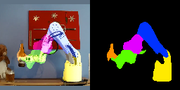
Figure 3: Visual results of our method tested on different scenarios, including human, hand, quadruped and robot arm.

Background Loss

As described in the last section, we treat the background as a special part segment and compute its features map and part mask. In practice, however, we observe that some background pixels can appear in the other part masks, causing noisy part segmentation. To address this problem, we include a novel background loss in the training to encourage clear partition between the object parts and the background. This is achieved by encouraging the background part to occupy as much image as possible, forcing the object parts to shrink into the most relevant region in the image. The background loss is thus defined as

$$\mathcal{L}_{\text{bg}}=\lambda_{\text{bg}}\left(\parallel M_{0}-1\parallel_{1}+\sum_{k=1}^{K}\parallel{M_{k}}\parallel_{1}\right)$$ (7)

which drives the values of the background mask close to one and the values of the other part masks close to zero. We apply this background loss to both the source parts $M^{s}_{k}$ and the retargeted parts $M^{s\rightarrow{}t}_{k}$. We find this loss essential for precise part segmentation with tight boundaries.

Transformation Loss

In our system, we expect each part transformation $T_{k}$ to be strongly correlated with the absolute pose of the part $k$ in the input image and thus has a clearly explainable physical meaning. More specifically, each part transformation $T_{k}=\left[A_{k}|\bm{t}_{k}\right]$ defines a coordinate system with the origin at $\bm{t}_{k}$ and the axes defined by $A_{k}$. We assume $\bm{t}_{k}$ to be located at the center of the part $k$ and the axis $A_{k}$ align with the longest and the shortest dimensions of the object part. We enforce such property in the training using a novel transformation loss defined as $\mathcal{L}_{\text{trf}}=\mathcal{L}_{\text{tran}}+\mathcal{L}_{\text{rots}}$, where

$$\mathcal{L}_{\text{tran}} =\lambda_{\text{tran}}\sum_{k=1}^{K}\parallel\bm{t}_{k}-\bm{\hat{u}}_{k}\parallel_{1}$$ (8)

$$\mathcal{L}_{\text{rots}} =\lambda_{\text{rots}}\sum_{k=1}^{K}\parallel A_{k}A_{k}^{T}-\Sigma_{k}\parallel_{F}$$ (9)

Since we do not have the ground-truth part poses, we estimate the reference transformation using the mean and the covariance of the part mask $M_{k}$ as

$$\bm{\hat{u}}_{k} =\frac{1}{z_{k}}{\sum_{\bm{u}\in{}\mathcal{U}}\bm{u}{M_{k}}(\bm{u})}$$ (10)

$$\Sigma_{k} =\frac{1}{z_{k}}{\sum_{\bm{u}\in{}\mathcal{U}}(\bm{u}-\bm{\hat{u}}_{k})(\bm{u}-\bm{\hat{u}}_{k})^{T}{M_{k}}(\bm{u})}$$ (11)

where $M_{k}(\bm{u})$ represents the mask value of the pixel located at $\bm{u}\in\mathcal{U}$ and $z_{k}=\sum_{\bm{u}\in{}\mathcal{U}}{M_{k}}(\bm{u})$ is a normalization constant. In this estimation, we only consider the pixels that have been clearly identified as part $k$ with a threshold $\zeta$, so that $\mathcal{U}=\{\bm{u}|M_{k}(\bm{u})>\zeta\}$. We choose $\zeta=0.02$ empirically in our implementation.

Figure 4: Visualization of the segmentation results. Left: The input image. Middle: The part images computed by our segment decoder. Right: The reconstructed image computed by part assembly.

Equivariance Loss

The estimation of the part transformations should be consistent across images and show equivariance to image transformations. Following the common practice of unsupervised landmark detection (Jakab et al., 2018; Zhang et al., 2018; Siarohin et al., 2019), we employ an equivariance loss in our training. Specifically, we transform the input image $I$ using a random transformation $T^{w}$. The encoder $\mathcal{E}$ then estimates part transformations for both the original image $I$ and the transformed image $I^{w}$. The equivariance loss is then defined as

$$\mathcal{L}_{\text{eq}}=\lambda_{\text{eq}}\sum_{k=1}^{K}\parallel T^{w}T_{k}-T^{w}_{k}\parallel_{1}$$ (12)

where $T_{k}$ and $T^{w}_{k}$ are the part transformations estimated from $I$ and $I^{w}$ respectively, and the 1-norm is computed with the transformation matrix treated as a vector.

Concentration Loss

To encourage the pixels belonging to the same object part to form a connected and concentrated component, we employ the geometry concentration loss suggested in SCOPS (Hung et al., 2019) to regularize the shape of part mask $M_{k}$. Specially, this concentration loss is computed as

$$\mathcal{L}_{\text{con}}=\lambda_{\text{con}}\sum_{k=1}^{K}\sum_{\bm{u}}\parallel\bm{u}-\bm{\bar{u}}_{k}\parallel^{2}_{2}\cdot{M_{k}}(\bm{u})/{z_{k}}$$ (13)

where

$$\bm{\bar{u}}_{k}=\frac{1}{z_{k}}\sum_{\bm{u}}\bm{u}{M_{k}}(\bm{u})$$ (14)

is the center of gravity of the part mask $M_{k}$, and $z_{k}=\sum_{\bm{u}}{M_{k}}(\bm{u})$ is a normalization constant. Unlike the transformation loss, we consider all the pixels in $M_{k}$ in this concentration loss. Note that the summation of Equation (13) excludes the part mask corresponding to the background. As shown in Fig. 2, we apply concentration loss to the part masks of the source parts $M^{s}_{k}$, the retargeted parts $M^{s\rightarrow{}t}_{k}$, and the canonical parts $M^{*}_{k}$.

4 Experiments

Our model is implemented using the the standard U-Net architecture. We include the details about the network structure and the training settings in the supplementary materials. We visually demonstrate the effectiveness of our co-part segmentation method on several test cases with large variation, including human, hand, quadruped, and robot arms in Figure 3, where the resulting part segments are rendered with different colors with the corresponding masks computed using hardmax $M_{k}(\bm{u})=\max_{l\in{0}\cup{}\mathcal{K}}D_{l}(\bm{u})$ instead of Equation (3). Additionally, Figure 4 illustrates the individual segment images computed by our network.

Our method is designed to extract parts that exhibit different affine transformations in the training image pairs, which is consistent with the behavior of semantically meaningful segmentation of a subject, such as a human body. The order of these parts is not determined in the unsupervised learning process. As in previous works, we manually label those parts after the model training. Notably, we only need to label the parts once, and the labels are consistent over all test images.

In the rest part of this section, we will introduce the ablation studies we performed to analyze the effectiveness of each loss component in our framework, and also the comparison with state-of-the-art co-part segmentation techniques.

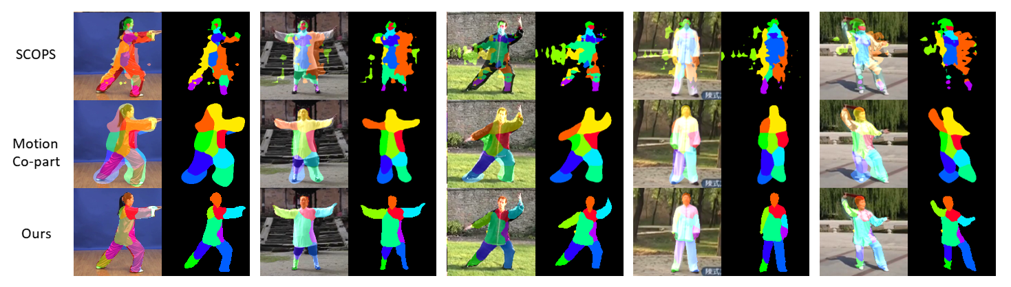
Figure 5: Visual result in Tai-Chi-HD. Motion Co-part and our method both produce relatively better and consistent part segmentation than SCOPS. Our segmentation are more compact and tightly aligned with image silhouette.

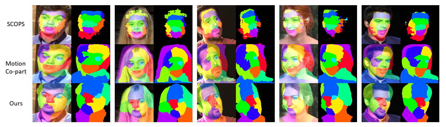
Figure 6: Visual result on VoxCeleb. All of the three methods produce consistent part segments, but our segmentation are more compact and tightly aligned with the image silhouette.

Table 1: The quantitative evaluation on the validation set of Tai-Chi-HD and VoxCeleb. The evaluation metrics are the foreground IOU and landmark regression MAE.

Dataset	Metric	SCOPS	Motion	Ours
			Co-part
Tai-Chi-HD	Landmark	411.38	389.78	326.82
	IoU	0.5485	0.7686	0.8724
VoxCeleb	Landmark	663.04	424.96	338.98
	IoU	0.5045	0.9135	0.9270

4.1 Datasets

Tai-Chi-HD.

Tai-Chi-HD dataset (Siarohin et al., 2019) is a collection of short videos with full-body Tai-Chi movements. $2981$ Tai-Chi videos were downloaded from YouTube. The videos were cropped and resized to a fixed resolution of $128\times 128$, while preserving the aspect ratio. There are $2746$ training videos and $235$ test videos. This dataset contains $5300$ images with ground truth landmarks ($18$ joints) generated using the method from Cao et al.(Cao et al., 2019). Only $300$ images with ground truth foreground segmentation mask are available.

Table 2: The quantitative evaluation on the validation set of Exercise. The evaluation metric is the part segment IoU.

Part	REM	N-REM	PSD	Flow	Ours
				Capsule
Full	0.298	0.321	0.697	-	0.793
Upper	0.347	0.319	0.574	0.690	0.759
Arm	0.125	0.220	0.391	-	0.465
Leg(L)	0.264	0.294	0.374	0.590	0.726
Leg(R)	0.222	0.228	0.336	0.540	0.642
Average	0.251	0.276	0.474	-	0.677

VoxCeleb.

The VoxCeleb dataset (Nagrani et al., 2017) is a large scale face dataset, which consists of $22496$ videos, extracted from YouTube. We follow the preprocessing described in  (Siarohin et al., 2019) to crop original video into several short sequences to guarantee that face can move freely in the image space with reasonable scale. All the cropped videos are then resized to $128\times 128$, again, preserving the aspect ratio. After the preprocessing, our dataset contains $15103$ training videos and $443$ test videos. The length of each video varies from $64$ to $1024$ frames. This dataset contains $5300$ images with ground truth landmarks ($68$ keypoints) generated using the method from Bulat et al.(Bulat & Tzimiropoulos, 2017). Similarly, only $300$ images with ground truth foreground segmentation mask are available.

Exercise.

Exercise dataset is a collection of paired images from two consecutive frames for full human body performing Yoga exercises. This dataset is originally collected by (Xue et al., 2016) from YouTube, and preprocessed with motion stabilization. We use the reorganized version of this dataset provided by (Xu et al., 2019), which contains $49356$ pairs of images for training. For this dataset, only $30$ images with ground truth part segmentation masks are available.

4.2 Metrics

Intersection Over Union

We use the commonly adopted mean intersection over union (IoU) metric to evaluate how similar our predicted segmentation is to the ground truth. The average IoU across all frames of the dataset is practically used. We use foreground IoU for the test on VoxCeleb and Tai-Chi-HD datasets due to the shortage of ground-truth part segmentation mask; while part IoU is used for the test on Exercise dataset.

Landmark Regression MAE

We use the landmark regression MAE metric to evaluate whether our method can generate consistent semantic part segmentation on different images. Following  (Hung et al., 2019), We first fit a linear regression model from the parts’ center of mass $\bm{\bar{u}}_{k}$ to ground truth landmarks using $5000$ annotated images, where $\bm{\bar{u}}_{k}$ is calculated using Equation 14, and then on the other $300$ images, we compute the mean average error (MAE) between regressed and ground truth landmark positions as the evaluation metric.

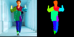
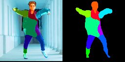
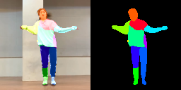
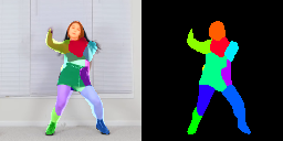
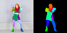
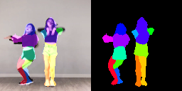
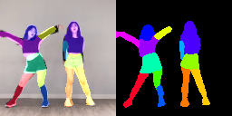
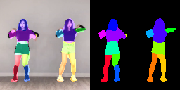
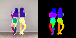
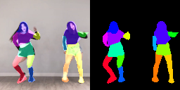
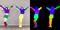
Figure 7: Top, Middle: Visual results of applying models trained on Tai-Chi-HD (top) and VoxCeleb (middle) to videos from YouTube. Bottom: Visual results of the model trained on a video with multiple characters.

4.3 Quantitative Comparison

We quantitatively compare our result with that of the state of the art methods for co-part segmentation, SCOPS (Hung et al., 2019), Motion Co-part (Siarohin et al., 2020), PSD (Xu et al., 2019), NEM (Greff et al., 2017), N-REM (Steenkiste et al., 2018) and Flow Capsules (Sabour et al., 2020), using both IoU and Landmark metrics.

We first compared our method with SCOPS and Motion Co-part using landmark regression and foreground IoU metrics on VoxCeleb and Tai-Chi-HD dataset, which have rich variation on background texture, actor’s appearance and body proportions, etc. To make a fair comparison, we train our model with $K=10$ in this test, which is consistent with the settings of the other methods. The results in Table 1 indicate that our method significantly improves the accuracy of foreground segmentation and can achieve more consistent and precise segmentation. As illustrated in Figures 5 and 6, our approach achieves more consistent part segmentation than SCOPS, where the main objects are clearly separated from the background. In the meanwhile, our results are aligned with image silhouette more tightly than Motion Co-part.

We further compare our method with PSD, NEM, R-NEM and Flow Capsule on the accuracy of co-part segmentation using the IoU metric on Exercise dataset. We train our model with $K=15$ segments in this comparison. As reported in Table 2, our model achieves a consistently better performance than the baselines.

4.4 Generalization

Our model can be trained with both single-video settings (hand, quadruped, and robot arm) and multiple-video settings (Tai-Chi-HD, VoxCeleb, and Exercise datasets), where in the latter case, each pair of images are extracted from the same random video during training. Models trained with multiple videos can be generalized to images of the same category but with difference appearance. For example, without further training, the models trained on Tai-Chi-HD and VoxCeleb datasets can be applied directly to videos downloaded from YouTube, as shown in the top two rows in Figure 7.

Moreover, it is rather straightforward to extend our method to support multiple subjects. The bottom row of Figure 7 demonstrates an example of such ability, where a model is trained on a video with two persons, and $K=17$ is used to accommodate additional potential part segments.

Table 3: Ablation study for different loss on Tai-Chi-HD.

Measures	w/o	w/o	w/o	w/o	w/o	Full
	$\mathcal{L}_{\text{vgg}}$	$\mathcal{L}_{\text{bg}}$	$\mathcal{L}_{\text{rots}}$	$\mathcal{L}_{\text{tran}}$	$\mathcal{L}_{\text{con}}$
Landmark	386.1	350.6	335.8	334.5	366.6	326.8
IoU	0.784	0.828	0.856	0.861	0.861	0.872

4.5 Ablation Study

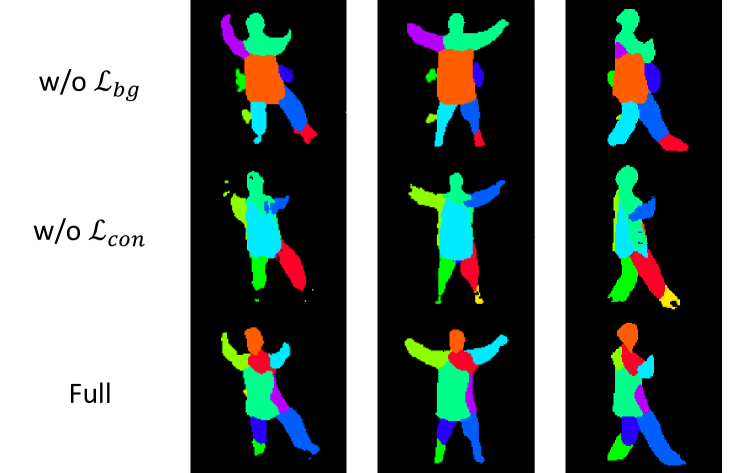
Figure 8: Visual comparison of segmentation results by using full loss, disable ${\cal L}_{con}$ and ${\cal L}_{bg}$ individually. Without ${\cal L}_{bg}$, background information distributed into many channels; while without ${\cal L}_{bg}$, the foreground segmentation have severe noisy.

We perform ablation studies to validate the contribution of each loss employed in our training. The comparison is conducted between the full training objective proposed in Sec.3.2 and its variants, each with one of the losses ($\mathcal{L}_{\text{vgg}}$, $\mathcal{L}_{\text{bg}}$, $\mathcal{L}_{\text{rots}}$, $\mathcal{L}_{\text{tran}}$, $\mathcal{L}_{\text{con}}$) disabled. We use Tai-Chi-HD dataset in these experiments, and the results are reported in terms of foreground IoU and landmark regression accuracy. Note that in the ablation study with $\mathcal{L}_{\text{vgg}}$, we only remove the VGG features from $\mathcal{L}_{\text{rec}}$ and keep the rest terms of Equation (5) unchanged. The results summarized in Table 3 reveal that all the losses are beneficial towards effective learning.

$\mathcal{L}_{\text{vgg}}$ is the most significant one among them, which influences both foreground extraction and part segmentation. Unlike the methods that generate images using field-based global warping operation (Siarohin et al., 2019; Sabour et al., 2020), our model cannot utilize the pixels of the input image directly to generate the target image, where the VGG features significantly facilitate the training and help achieve a good performance.

$\mathcal{L}_{\text{bg}}$ is another critical term of our objective design, which enforces all the background information to be embedded in the background channel, thus consequently ensuring the segmentation tightly aligned with the foreground silhouette. As shown in Figure 8, the segmentation trained without this loss can be noisy with background pixels mislabeled as a part of object segments.

Similar to the results reported in (Hung et al., 2019), we find $\mathcal{L}_{\text{con}}$ guarantees the semantic correctness of the segmented parts through penalizing vague and scattered partition in each channel. This conforms to our ablation study that $\mathcal{L}_{\text{con}}$ has obvious effect on Landmark regression accuracy. More visual comparison result can be found in Figure 8.

As illustrated in Figure 9, $\mathcal{L}_{\text{rots}}$ and $\mathcal{L}_{\text{tran}}$ play a critical role in bringing the estimated part transformation with explainable meaning. The part transformations learned without these losses only loosely correlate to the global pose of the parts, while the transformations estimated using our model align with the motion of the object parts. We find these loss terms very effective when the transformation of each part can be clearly defined, such as in the case of human limbs in the Tai-Chi-HD dataset. Nonetheless, these loss terms take only marginal effect on faces in the VoxCeleb dataset, though we kept this term as a part of a uniform training process.

Package pdftex.def Error: File ‘figures/ablation.pdf’ not found: using draft setting.

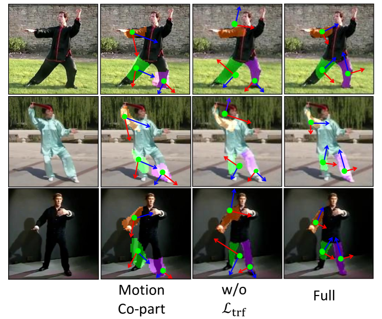
Figure 9: Visual comparison for the interpretability of intermediate affine transformations, which are generated using our method with full loss, disable ${\cal L}_{\text{trf}}$ and method in Motion Co-part respectively.

5 Discussion

In this paper, we have proposed an unsupervised Co-part segmentation approach, which leverages shape correlation information between different frames in the video to achieve semantic part segmentation. We have designed a novel network structure which achieves self-supervision through a dual procedure of part-assembly to form a closed loop with part-segmentation. Additionally, we have developed several new loss functions that ensure consistent, compact and meaningful part segmentation and the intermediate transformations with clear explainable physical meaning. We have demonstrated the advantages of our method through a host of studies.

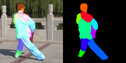
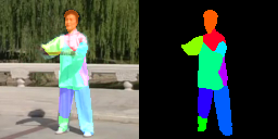
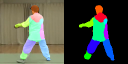
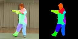
Figure 10: Failure case. Due to the lack of temporal information, our method can fail in inferring occluded parts and may incorrectly label the limbs when a person turn around.

We empirically choose weights in our training to balance the magnitude of each loss term in a preliminary training, except for the image reconstruction loss, which is an order of magnitude larger than the other regularization terms due to its critical role in the training. The performance of our model is not sensitive to the specific choice of these loss weights, and similar video categories can share the loss weights. In order to make a fair comparison, we deliberately use different $K$ in some of the experiments to ensure consistency with the baseline methods, but the performance of the method is not sensitive to the specific value of a large enough $K$. For example, we can achieve correct segmentation using an empirical value of $K=15$ in all the test cases discussed in the paper.

Several lines are open for future research. First, As showed in Figure 10, due to the lack of temporal information, our method can fail in inferring occluded parts and may incorrectly label the limbs when a person turns around. It would be a valuable extension of the current framework to train with image sequences or videos to address such inconsistency issues using the time coherence information embedded in the video. Second, although our method allows moderate background motions as exhibited in Tai-Chi-HD and VoxCeleb datasets during training, dramatic background change can interfere the training stage and degrade the performance. Extending our method to support training on videos with dramatic background change is a viable future work. Another interesting direction would be additionally identifying joint positions, which would significantly support a more diverse range of applications. Lastly, extending the study of co-part segmentation to 3D makes another meaningful future work.

References

- Bulat & Tzimiropoulos (2017) Bulat, A. and Tzimiropoulos, G. How far are we from solving the 2d & 3d face alignment problem?(and a dataset of 230,000 3d facial landmarks). In Proceedings of the IEEE International Conference on Computer Vision, pp. 1021–1030, 2017.
- Cao et al. (2019) Cao, Z., Hidalgo, G., Simon, T., Wei, S.-E., and Sheikh, Y. Openpose: realtime multi-person 2d pose estimation using part affinity fields. IEEE Transactions on Pattern Analysis and Machine Intelligence, 43(1):172–186, 2019.
- Chang & Demiris (2018) Chang, H. J. and Demiris, Y. Highly articulated kinematic structure estimation combining motion and skeleton information. IEEE Transactions on Pattern Analysis and Machine Intelligence, 40(9):2165–2179, 2018.
- Collins et al. (2018) Collins, E., Achanta, R., and Susstrunk, S. Deep feature factorization for concept discovery. In Proceedings of the European Conference on Computer Vision, pp. 336–352, 2018.
- Eigen & Fergus (2015) Eigen, D. and Fergus, R. Predicting depth, surface normals and semantic labels with a common multi-scale convolutional architecture. In Proceedings of the IEEE International Conference on Computer Vision, pp. 2650–2658, 2015.
- Eslami & Williams (2012) Eslami, S. and Williams, C. A generative model for parts-based object segmentation. Advances in Neural Information Processing Systems, 25:100–107, 2012.
- Greff et al. (2017) Greff, K., van Steenkiste, S., and Schmidhuber, J. Neural expectation maximization. In Advances in Neural Information Processing Systems, volume 30, pp. 6691–6701, 2017.
- Güler et al. (2018) Güler, R. A., Neverova, N., and Kokkinos, I. Densepose: Dense human pose estimation in the wild. In Proceedings of the IEEE Conference on Computer Vision and Pattern Recognition, pp. 7297–7306, 2018.
- Hung et al. (2019) Hung, W.-C., Jampani, V., Liu, S., Molchanov, P., Yang, M.-H., and Kautz, J. Scops: Self-supervised co-part segmentation. In Proceedings of the IEEE Conference on Computer Vision and Pattern Recognition, pp. 869–878, 2019.
- Jakab et al. (2018) Jakab, T., Gupta, A., Bilen, H., and Vedaldi, A. Unsupervised Learning of Object Landmarks through Conditional Image Generation. Advances in Neural Information Processing Systems, 31:4016–4027, 2018.
- Johnson et al. (2016) Johnson, J., Alahi, A., and Fei-Fei, L. Perceptual losses for real-time style transfer and super-resolution. In Proceedings of the European Conference on Computer Vision, pp. 694–711, 2016.
- Kanazawa et al. (2018) Kanazawa, A., Black, M. J., Jacobs, D. W., and Malik, J. End-to-end recovery of human shape and pose. In Proceedings of the IEEE Conference on Computer Vision and Pattern Recognition, pp. 7122–7131, 2018.
- Keuper et al. (2015) Keuper, M., Andres, B., and Brox, T. Motion trajectory segmentation via minimum cost multicuts. In Proceedings of the IEEE International Conference on Computer Vision, December 2015.
- Khan et al. (2015) Khan, K., Mauro, M., and Leonardi, R. Multi-class semantic segmentation of faces. In Proceedings of the IEEE International Conference on Image Processing, pp. 827–831, 2015.
- Lathuilière et al. (2020) Lathuilière, S., Tulyakov, S., Ricci, E., Sebe, N., et al. Motion-supervised co-part segmentation. arXiv preprint arXiv:2004.03234, 2020.
- Lee & Seung (1999) Lee, D. D. and Seung, H. S. Learning the parts of objects by non-negative matrix factorization. Nature, 401(6755):788–791, 1999.
- Nagrani et al. (2017) Nagrani, A., Chung, J. S., and Zisserman, A. Voxceleb: a large-scale speaker identification dataset. 2017.
- Nguyen et al. (2013) Nguyen, T. D., Tran, T., Phung, D., and Venkatesh, S. Learning parts-based representations with nonnegative restricted boltzmann machine. In Asian Conference on Machine Learning, pp. 133–148, 2013.
- Ochs et al. (2014) Ochs, P., Malik, J., and Brox, T. Segmentation of moving objects by long term video analysis. IEEE Transactions on Pattern Analysis and Machine Intelligence, 36(6):1187–1200, 2014.
- Ross & Zemel (2006) Ross, D. A. and Zemel, R. S. Learning parts-based representations of data. Journal of Machine Learning Research, 7(11), 2006.
- Ross et al. (2010) Ross, D. A., Tarlow, D., and Zemel, R. S. Learning articulated structure and motion. International Journal of Computer Vision, 88(2):214–237, 2010.
- Sabour et al. (2020) Sabour, S., Tagliasacchi, A., Yazdani, S., Hinton, G. E., and Fleet, D. J. Unsupervised part representation by flow capsules. arXiv preprint arXiv:2011.13920, 2020.
- Siarohin et al. (2019) Siarohin, A., Lathuilière, S., Tulyakov, S., Ricci, E., and Sebe, N. First order motion model for image animation. December 2019.
- Siarohin et al. (2020) Siarohin, A., Roy, S., Lathuilière, S., Tulyakov, S., Ricci, E., and Sebe, N. Motion-supervised co-part segmentation. arXiv e-prints, pp. arXiv–2004, 2020.
- Simonyan & Zisserman (2015) Simonyan, K. and Zisserman, A. Very deep convolutional networks for large-scale image recognition. In Proceedings of the International Conference on Learning Representations, 2015.
- Steenkiste et al. (2018) Steenkiste, v. S., Chang, M., Greff, K., and Schmidhuber, J. Relational neural expectation maximization: Unsupervised discovery of objects and their interactions. Proceedings of the International Conference on Learning Representations, 2018.
- Sturm et al. (2011) Sturm, J., Stachniss, C., and Burgard, W. A probabilistic framework for learning kinematic models of articulated objects. Journal of Artificial Intelligence Research, 41:477–526, 2011.
- Sun & Savarese (2011) Sun, M. and Savarese, S. Articulated part-based model for joint object detection and pose estimation. In Proceedings of the International Conference on Computer Vision, pp. 723–730, 2011.
- Wang & Yuille (2015) Wang, J. and Yuille, A. L. Semantic part segmentation using compositional model combining shape and appearance. In Proceedings of the IEEE Conference on Computer Vision and Pattern Recognition, pp. 1788–1797, 2015.
- Xu et al. (2019) Xu, Z., Liu, Z., Sun, C., Murphy, K., Freeman, W. T., Tenenbaum, J. B., and Wu, J. Unsupervised discovery of parts, structure, and dynamics. In Proceedings of the International Conference on Learning Representations, 2019.
- Xue et al. (2016) Xue, T., Wu, J., Bouman, K. L., and Freeman, W. T. Visual dynamics: Probabilistic future frame synthesis via cross convolutional networks. 2016.
- Yan & Pollefeys (2008) Yan, J. and Pollefeys, M. A factorization-based approach for articulated nonrigid shape, motion and kinematic chain recovery from video. IEEE Transactions on Pattern Analysis and Machine Intelligence, 30(5):865–877, 2008.
- Zhang et al. (2018) Zhang, Y., Guo, Y., Jin, Y., Luo, Y., He, Z., and Lee, H. Unsupervised discovery of object landmarks as structural representations. In Proceedings of the IEEE Conference on Computer Vision and Pattern Recognition, pp. 2694–2703, June 2018.
- Zhou et al. (2019) Zhou, Y., Barnes, C., Jingwan, L., Jimei, Y., and Hao, L. On the continuity of rotation representations in neural networks. In Proceedings of the IEEE Conference on Computer Vision and Pattern Recognition, June 2019.