dFDA-VeD: A Dynamic Future Demand Aware Vehicle Dispatching System

Yang Guo¹, Tarique Anwar¹, Jian Yang^1,2, and Jia Wu¹ 1. Department of Computing, Macquarie University, Australia
2. College of Computer Science and Technology, Dong Hua University, P.R. China.
yang.guo5@students., tarique.anwar@, jian.yang@, jia.wu@mq.edu.au

Abstract.

With the rising demand of smart mobility, ride-hailing service is getting popular in the urban regions. These services maintain a system for serving the incoming trip requests by dispatching available vehicles to the pickup points. As the process should be socially and economically profitable, the task of vehicle dispatching is highly challenging, specially due to the time-varying travel demands and traffic conditions. Due to the uneven distribution of travel demands, many idle vehicles could be generated during the operation in different subareas. Most of the existing works on vehicle dispatching system, designed static relocation centers to relocate idle vehicles. However, as traffic conditions and demand distribution dynamically change over time, the static solution can not fit the evolving situations. In this paper, we propose a dynamic future demand aware vehicle dispatching system. It can dynamically search the relocation centers considering both travel demand and traffic conditions. We evaluate the system on real-world dataset, and compare with the existing state-of-the-art methods in our experiments in terms of several standard evaluation metrics and operation time. Through our experiments, we demonstrate that the proposed system significantly improves the serving ratio and with a very small increase in operation cost.

Vehicle Re-balancing, Mobility-on-Demand, Ride Hailing Services, Vehicle Dispatching

^†^†booktitle: MobiQuitous 2020 - 17th EAI International Conference on Mobile and Ubiquitous Systems: Computing, Networking and Services (MobiQuitous ’20), December 7–9, 2020, Darmstadt, Germany^†^†price: 15.00^†^†doi: 10.1145/3448891.3448912^†^†ccs: Applied computing Transportation^†^†ccs: Mathematics of computing Graph algorithms

1. Introduction

Mobility and mobility-on-demand services are major concerns of smart transportation. Mobility services exist in cities since long in the form of public transportation, and mobility-on-demand services were limited to renting cars, offered by companies like Hertz and Avis. However, as we strive to make our cities smarter, over the past 10 years, we have seen the evolution of mobility-on-demand services into many new, effective, and more convenient forms. These services are increasingly being promoted as an influential strategy to address the challenges of urban transportation in large and fast-growing cities. Evolving from the traditional taxi service model, today companies like Uber, Lyft, Ola, Didi and many others are popular as ride-hailing mobility-on-demand service providers in many cities globally. These services are facilitated by the recent advancements in communication technologies and widely used GPS-enabled mobile devices. Customers can send trip requests to the service provider from their mobile devices in real time. Upon receiving the requests, the vehicle dispatching system of the service provider assigns available vehicles to serve the trip requests. While in progress, the system keeps track of geographic location of both the customer and the vehicle in order to maintain an updated information dynamically, and provide a smooth service. One major problem in the vehicle dispatching system is to find the most suitable vehicle to serve a trip request in such a way that results into the highest overall social and economical benefit. With rapid developments taking place currently in the field of Internet of Things (IoT), especially vehicle-to-anything (V2X), the future will have the availability of more data of vehicles and traffic, with high accuracy (chen2017vehicle). Using the dynamic traffic data on the roads and predicting the future travel demands are major aids in making estimations of benefit while serving a trip request, and thus have a high potential to improve the decision making of mobility-on-demand services.

Being an important component of the mobility-on-demand services, research on vehicle dispatching system has been under attention since quite some time (dantzig1959truck; toth2002vehicle; pisinger2007general; kool2018attention). Several concerns have been studied since then (wang2019ridesourcing). One major concern is to deal with the uneven geographic distribution of trip requests and available vehicles. Quite often there arise geographic areas of low trip demand with over-supplied vehicles, at the same time when there are other areas of high trip demand with under-supplied vehicles. To address this issue, efficient relocation of idle vehicles from areas of low demand to those of high demand has been an important problem (guo2020FDAVeD). Addressing this issue is crucial to improve the serving ratio of incoming trip requests. Vazifeh et al. (vazifeh2018addressing) gave the lower bound of fleet size to serve all travel requests in an ideal scenario, considering that all travel requests are known in advance. Having this given knowledge, relocating the idle vehicles to areas with high trip demand potential could significantly improve the serving ratio. For this relocation, Wallar et al. (wallar2018vehicle) first found fixed relocation centers for the serving area based on maximum waiting time. They treat the road graph $G=(V,E)$ as a static graph, shown as Fig. 1(a), and formulated the relocation center searching as an Integer Linear Programming problem (ILP). Due to its high computational complexity, this method requires so long running time that can not be used for online relocation in a real time scenario. Our previous work (guo2020FDAVeD) can be used online to deal with only the dynamic traffic conditions, shown as the changing attribute of edges in the road graph $G^{t}=(V,E,W_{e}^{t})$ (Fig. 1(b)). Some traditional graph partitioning algorithms (von2007tutorial; Lin2010power) could also partition the graph efficiently, but only consider the weights on edges.

Refer to caption — Figure 1. Illustration of static and dynamic road graphs. The directed graphs show the road network of a serving area, where vertices represent the pickup/dropoff points, and edges represent the directed path connecting the pickup/dropoff points. The colors highlight the different attributes on vertices and edges. The vertices in red color denote the points that have under-supplied vehicles and the vertices in blue color denote the points that over-supplied vehicles. The color of edges denotes the travel time in respective ways. (a) Static Road Graph $G=(V,E)$ . The attributes of both vertices and edges do not change over time in this graph. (b) Dynamic-edge Road Graph $G^{t}=(V,E,W_{e}^{t})$ . The attributes of edges change over time in this graph. The changing color of edges in different timestamps show the time-varying attributes $W_{e}^{t}$ of edges. (c) Dynamic Graph $G^{t}=(V_{t},E_{t},W_{v}^{t},W_{e}^{t})$ . The attributes of both vertices and edges change over time.

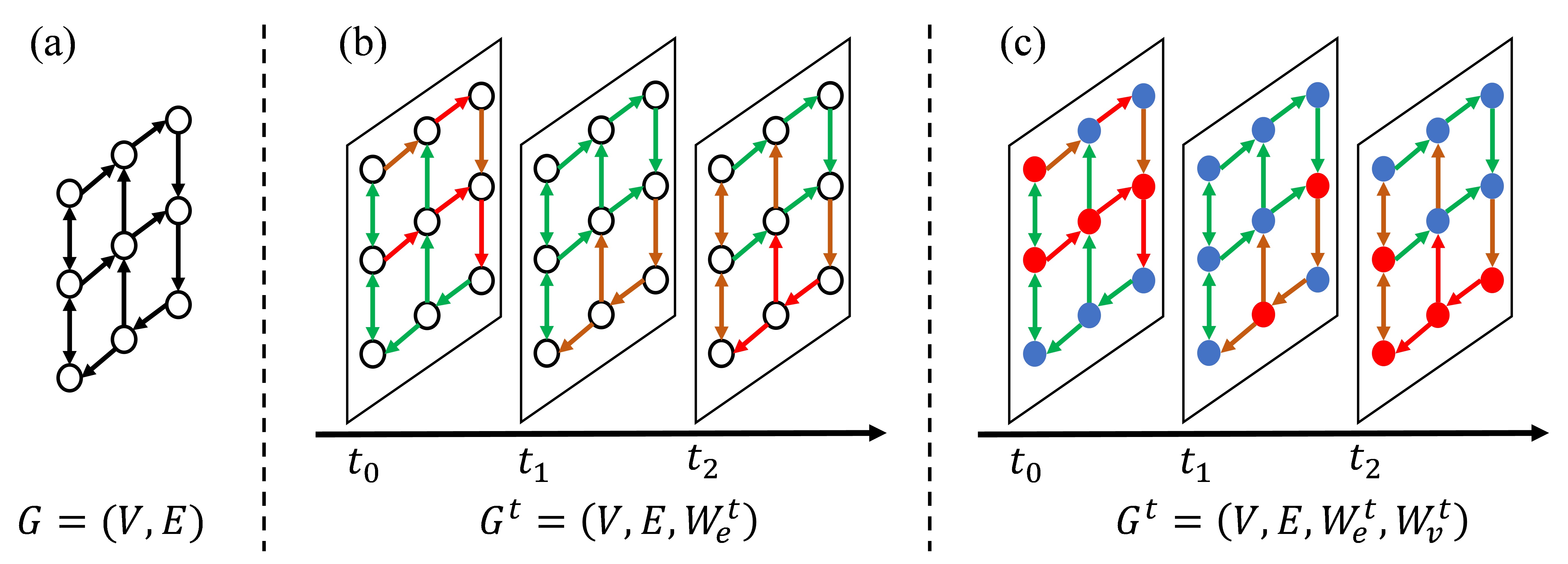
In a vehicle dispatching system, road graph have dynamic traffic information on edges ( $W_{e}^{t}$ ) and trip request information on vertices ( $W_{v}^{t}$ ), as shown in Fig. 1(c). The existing research does not effectively use both these information for idle vehicle relocation. Therefore it demands further research for a vehicle dispatching system that considers the dynamic information of travel demand on the nodes and traffic on the edges, and that could search relocation centers online based on the dynamic information. The online relocation in this manner will find the most suitable relocation centres and effectively improve the serving quality from different perspectives. There are two main challenges to achieve this. The main challenge in addressing this existing limitation is to simultaneously consider both traffic and demand information for identifying appropriate vehicle relocation centres dynamically, and develop an online real-time relocation mechanism.

To address the existing limitations, in this paper, we propose a dynamic future demand aware vehicle dispatching system (called dFDA-VeD). It is designed for urban on-demand mobility service and can efficiently make decision for both vehicle dispatching and idle vehicle relocation. Unlike present works (wallar2018vehicle; guo2020FDAVeD; von2007tutorial; Lin2010power), dFDA-VeD could partition road graph and search appropriate relocation centers online based on both traffic and demand information. Overall, we make the following main contributions:

–

We propose a vehicle dispatching system, called dFDA-VeD, which could dynamically search idle vehicle relocation centers online, considering the attributes on both vertices and edges of a road graph.
–

We develop a dynamic road graph partitioning based optimization objective function that considers both real-time traffic and travel demand information in order to effectively relocate the vehicles.
–

We propose an algorithm to achieve a local optimum in order to solve the optimization objective function, and also theoretically prove its convergence. The local optimum is able approach the global optimum by parallel processing of multiple instances.
–

We perform extensive experiments on a real dataset and compare our results with the existing systems. Results show that our dynamic idle vehicle relocation based dispatching system dFDA-VeD outperforms the state-of-the-art vehicle dispatching systems in terms of passenger serving ratio with an increase in a very small operating cost.

The rest of the paper is organized as follows. Section 2 presents the related works in vehicle dispatching system and idle vehicle relocation task. Then we give the problem formulation in Seciton 3. The dFDA-VeD system is introduced in Section 4. Section LABEL:sec:experiment explore the performance of the dFDA-VeD system against real-world taxi data, and compared it with several baselines. Finally we conclude the paper in Section LABEL:sec:conclusion, along with a brief discussion on the future research directions.

2. Related Work

Vehicle dispatching problem has been studied for decades (dantzig1959truck; toth2002vehicle; pisinger2007general; kool2018attention; wang2019ridesourcing). The objective of a dispatching system is to provide better service for the passengers, specifically higher serving ratio, shorter waiting time, lower cost and so on. Dandl et al. (dandl2018comparing) converted the dispatching problem to two bipartite matching problem: vehicle-to-user and relocation assignments. Liu et al. (liu2019globally) periodically get the optimal result in offline using predicted demands and use the offline results to guide the online dispatching. The two bipartite matching problem and future demands are both considered in our previous paper (guo2020FDAVeD). Tang et al. (tang2019deep) and Al et al. (al2019deeppool) proposed reinforcement learning method to solve the vehicle dispatching problem. Kim et al. (kim2020multi) considered multi-objective vehicle dispatching problem and use minimum cost maximum flow algorithm to solve. Liu et al. (liu2020mobility) considers the mobility ride demand on roadside which are not sent to centralised platform. These researchers consider different objective and methods to improve the dispatching service quality. In this paper, we handle both the vehicle–request matching and idle vehicle relocation problem, and make several contributions on the latter one.

For a city, it is important to know the minimum number of vehicles that can serve the travel requests in the region. In 2018, the minimum number of vehicles to serve a city is addressed when all travel requests are known in advance (vazifeh2018addressing). They transferred the problem to find the minimum path cover for directed acyclic graph, where nodes stand for trips. This scenario could be treated as a special case that all idle vehicles are relocated to the passengers’ pickup location in time. It shows the power of a perfect idle vehicle relocation strategy. However, in real urban on-demand mobility application, the travel demands are received in real time. In this section, we introduce the two kinds of methods to handle idle vehicle relocation problem: machine learning and other methods.

Machine learning methods are used to design end-to-end machine solutions to relocate idle vehicles. Li et al. (li2018dynamic) designed a reinforcement learning technique to reposition bikes in a bike-sharing system. In their methods, the whole serving area are partitioned to several cluster, and a spatio-temporal reinforcement learning model are trained to learn an optimal inner-cluster reposition policy for each cluster. Holler et al. (Holler2019Deep) consider the problem from a system-centric perspective. They built a central fleet management agent to make decision for all drivers and trained policies using Deep Q-Networks (mnih2015human) and Proximal Policy Optimization (schulman2017proximal) algorithms. For the end-to-end machine learning solutions, the searching space is huge and hard to explain why the learned policy works. It needs a long time to train the optimal policy on simulation system before running online. However, using traditional optimization method, usually mathematically proof can be given from theory. Different from the machine learning methods, we use traditional optimization method to solve the idle vehicle relocation problem and give mathematical proof to guarantee the local optimal for the optimization.

Optimization and heuristic methods treat the idle vehicle relocation problem as an optimization problem and use traditional or heuristic methods to find the optimal solution. To relocate the idle vehicle, the relocation centers and subareas should be searched and idle vehicles should be redistributed the vehicles between subareas. Volkov et al. (volkov2012markov), Dandl et al. (dandl2018comparing) partitioned serving area based on pickup/dropoff points’ physical distance. Wallar et al. (wallar2018vehicle) divided the serving area based on travel time and search the minimum number of relocation centers using linear programming methods. This method takes a long time to calculate the optimal results and can only be used in offline. Guo et al. (guo2020FDAVeD) proposed a heuristic method to search the relocation centers based on the traffic conditions, which could find relocation centers in an efficient way. However, they do not consider effect of the travel demand distribution.

Our work is different from the existing idle vehicle relocation in two aspects: (1) The existing works only consider the static information (volkov2012markov; dandl2018comparing; wallar2018vehicle) or dynamic traffic information (guo2020FDAVeD). Unlike them, we consider both the dynamic traffic conditions and travel demands to search the relocation centers, and give an objective function to search optimal relocation centers. (2) Most previous studies decide the relocation centers offline (volkov2012markov; dandl2018comparing; wallar2018vehicle; guo2020FDAVeD), whereas we propose an online relocation center searching method that meets the online dispatching requirement, and guarantee a local optimal result for the objective function.

3. Problem Formulation

3.1. Preliminaries

The vehicle dispatching system contains two entities: passengers and vehicles. Passengers send the trip requests to the dispatching system in a streaming fashion. After receiving a set of trip requests in a batch time, the system needs to match these requests with available vehicles. The dispatching problem is to find the best assignment plan for vehicles to serve the maximum number of requests. Here we formulate the problem with following definitions.

Definition 0 (Trip Request).

A trip request $T_{i}$ , defined as a tuple ( $t_{i}^{p},l_{i}^{p},l_{i}^{d}$ ), is a trip requested by a passenger at time point $t_{i}^{p}$ (the earliest time when the passenger can be picked up) from location $l_{i}^{p}$ , to drop off at location $l_{i}^{d}$ . A set of trip requests during a particular time interval (e.g., 1 minute) is denoted by $\mathcal{T}=\{T_{1},T_{2},...,T_{k}\}$ . $\blacksquare$

Definition 0 (Road Graph).

A road graph $G=(V,E,W_{v}^{t},W_{e}^{t})$ is a directed graph presenting the road network topology, comprising a set of vertices $V=\{v_{1},v_{2},...,v_{n}\}$ , which are pickup/dropoff points of trip requests, connected by the set of directed edges $E=\{e_{1},e_{2},...,e_{m}\}$ , which are paths in the actual road network. $W_{v}^{t}$ is the set of vertex attributes, which are pickup-dropoff gaps (defined later in Definition 3.3) of corresponding vertices at time point $t$ . $W_{e}^{t}$ is the set of edges weights or attributes, which are travel times on corresponding edges at time point $t$ . $\blacksquare$

Definition 0 (Pickup–dropoff Gap).

The pickup–dropoff gap $g_{i}^{t}$ is the difference between the number of pickup and dropoff demands for point $v_{i}$ in the time window $[t,t+t_{r})$ . Here $t_{r}$ is the time length for relocating idle vehicles to their destinations. $\blacksquare$

Definition 0 (Served Trip).

A trip request $T_{i}$ is called as a served trip if the passenger is actually picked up between $t_{i}^{p}$ and $t_{i}^{p}+\Delta$ , where $\Delta$ is a pre-defined serving threshold (passenger’s maximum waiting time). The set of trip requests already served by the dispatching system is denoted by $\mathcal{T}_{served}$ , which is a sub set of the total set of trip requests $\mathcal{T}$ . Mathematically, $\mathcal{T}_{served}=\{T_{i}|t_{i}^{p}\leq\,^{a}t_{i}^{p}\,\leq t_{i}^{p}+\Delta\}$ , where ${}^{a}t_{i}^{p}$ is the actual pickup time. $\blacksquare$

Definition 0 (Served Trip Ratio).

Given the set of served trips $\mathcal{T}_{served}$ and all the trip requests $\mathcal{T}$ , the serving ratio $R$ of the centralized vehicle dispatching system is defined as the ratio of $\mathcal{T}_{served}$ to $\mathcal{T}$ , i.e., $R=\frac{|\mathcal{T}_{served}|}{|\mathcal{T}|}$ . $\blacksquare$

3.2. Problem Definition

The problem considered in this paper is to develop a vehicle dispatching system that achieves a high serving ratio by dynamically relocating idle vehicles from over-supplied areas to under-supplied areas. A vehicle $v_{i}\in\mathcal{V}$ can serve only one trip request at one time. It can start to serve a new trip request only after it has arrived at the destination of its last trip. With a given number of vehicles $n_{v}$ on a road graph $G$ , a set of real-time trip requests $\mathcal{T}$ in a batch, a set of historical trips $\mathcal{H}$ completed, the objective of the centralized vehicle dispatching system is to serve the maximum number of real-time trip requests $\mathcal{T}$ by dynamically relocating the idle vehicles, and thus achieve a high serving ratio $R$ .

(1)

\displaystyle\begin{aligned} &\mbox{maximize }\;\;R=\frac{|\mathcal{T}_{served}|}{|\mathcal{T}|},\\ &\mbox{subject to }\;\;\forall t_{i}\in\mathcal{T}_{served},\;\;t_{i}^{p}\leq\,^{a}t_{i}^{p}\leq t_{i}^{p}+\Delta\end{aligned}

4. Proposed vehicle dispatching system

This section presents the proposed vehicle dispatching system dFDA-VeD. We present the overall framework of dFDA-VeD in Section 4.1 and the detailed method for the future-demand-aware dynamic relocation of idle vehicles in Section 4.2.

4.1. Dispatching system

We solve the problem of vehicle dispatching in a ride-hailing mobility-on-demand service by developing a dynamic future demand aware vehicle dispatching system (dFDA-VeD). Fig. 2 shows the overall framework of the dFDA-VeD system. It starts with an offline phase of preprocessing, and then follows on to an online phase of continuously serving the realtime trip requests with available vehicles. The offline phase pre-processes the road graph data and trains a point-level travel demand prediction model based on the historical data only once in the beginning. The online phase dynamically partitions the available road graph into sub-graphs, dispatches vehicles for incoming requests, and also relocates idle vehicles based on potential future demands. The two phases of our dFDA-VeD system and individual modules in them are briefly explained below. As our primary focus in this paper is the dynamic relocation of idle vehicles, we skip the complete details of other tasks and modules in this paper, and present our vehicle relocation method in the next section in detail. For other tasks and modules, we follow the ideas from our previous paper (guo2020FDAVeD) (refer to this paper for details).

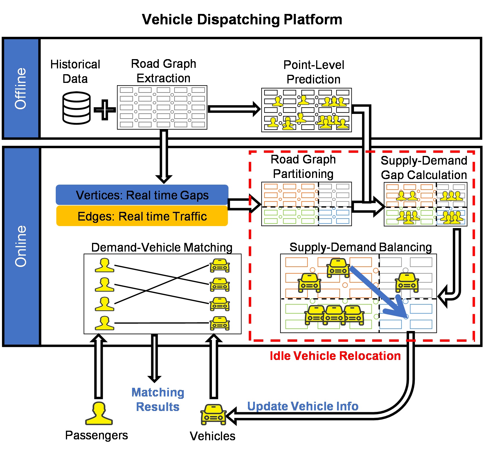
4.1.1. Offline Phase

There are two modules in the offline phase: extract road graph module and point-level demand prediction module. The first module extracts the road graph which is a fundamental information required in the online phase. The second module trains a point-level demand prediction model, used in the supply–demand gap calculation module (discussed later) in online phase. These two modules are briefly discussed below.

Road graph extraction module constructs the road graph $G=(V,E)$ for the dispatching system, where $G$ is a directed graph, $V$ is the set of vertices representing the pickup/dropoff points in the serving area, and $E$ is the set of edges representing the directed paths connecting the pickup/dropoff points in the serving area. The road graph $G$ is fundamental for all other modules.

Point-level prediction module uses the point-level historical average of travel demands as predictions for the prediction model. The prediction model is used later in the online phase to get predictions for the future travel demands at different pickup/dropoff points and calculate the supply-demand gap.

4.1.2. Online Phase

The online phase is the key to dispatch vehicles and relocate idle vehicles continuously in real-time. These two tasks are performed by four modules: graph partition module, supply–demand gap calculation module, demand–vehicle matching module and supply–demand balancing module. The graph partition module dynamically partitions $G$ based on both real-time traffic and travel demand. The supply–demand gap of each subarea is calculated by the supply–demand gap calculation module. Then, the vehicle dispatching task is handled by the demand–vehicle matching module. The supply–demand balancing module is used to address the idle vehicle relocation task. These four modules are briefly discussed below.

Road graph partition module is used to partition the set of vertices $V$ for the whole serving area in to $k$ subareas ${A_{1},A_{2},...,A_{k}}$ . The input of this module is the road graph $G=(E,V,W_{e}^{t},W_{v}^{t})$ . Here $W_{e}^{t}$ stands for the travel time on each directed edge $e_{i}\in E$ . $W_{v}^{t}$ stands for the pickup-dropoff gap for each vertex $v_{i}\in V$ . For any vertex $v_{i}$ in the road graph $G=(E,V)$ at a specific time-point $t$ , there are $pk_{i}$ and $dp_{i}$ standing for the number of pickup and dropoff demands at this vertex during the specific time interval $(t,t+\Delta)$ . Then the we calculate $g_{i}=pk_{i}-dp_{i}$ , which stands for the gap between pickup and dropoff demands in this time interval. Here, the pickup–dropoff demand gap is the attribute of vertices $V$ , so $W_{v}=\{g_{i}|i=1,...,n\}$ . The subarea set $\{A_{i}\|i=1,2,...,k\}$ is the partition of vertices set $V$ , which means to limitations: firstly, $\bigcup_{i=1}^{k}A_{i}=V$ ; secondly, $\forall i\neq j,A_{i}\cap A_{j}=\emptyset$ . The objective function for partitioning the road graph and the algorithm to optimise the objective function are presented in Section 4.2.

Supply–demand gap calculation module use the model trained in offline to predict the travel demand at point level, and then calculate the corresponding region level supply–demand gap for the each subarea $A_{i}$ . The supply–demand gap is used in supply–demand balancing module to relocate the idle vehicles.

Demand–vehicle matching module uses Hopcroft–Karp algorithm (hopcroft1973an) to find the maximum matching between the received trip requests in a short batch and available vehicles at that time. The available vehicles for a specific trip request are the vehicles that can arrive at the passenger’s pickup point in $\Delta$ seconds.

Supply–demand balancing module relocates the idle vehicles to undersupply subareas. It starts with a search for idle vehicles. The idle vehicles are the free vehicles in over-supplied subareas. Then it follows to finding the maximum matching between the idle vehicles and the relocation centers of the under-supplied subareas. Note that the relocation centres are identified dynamically in the road graph partitioning module. The matching results are used to relocate the idle vehicles, and balance the vehicle supply in the whole serving area.

4.2. Dynamic Idle Vehicle Relocation

Relocating idle vehicles is very important to deal with the dynamically changing travel demand and supply of vehicles in different sub-areas of a serving area. This task would effectively re-balance the vehicles in different subareas according to the demand and supply. It requires the relocation destinations (a.k.a centres) to be firstly identified in order to make the decision. The serving area could be partitioned based on the passengers’ maximum waiting time into subareas with some centres to be potential relocation destinations (wallar2018vehicle; guo2020FDAVeD). Specifically, the vehicles at relocation centers should be able to serve the trip requests in the whole serving area taking a minimum time. As the traffic conditions and the travel demands continuously change in a dynamic manner, the relocation centers also need to be updated with the changing conditions, so that they can keep serving the entire effective area in minimum time. In order to achieve this objective, we define a cost function $F(\mathcal{C},V,W_{v})$ to evaluate the performance of a set of searched relocation centers. The function is shown in Equation 4.2, where $d(c_{j},v_{i})$ is a distance function considered as the travel time from point $c_{j}$ to $v_{i}$ , weighted by an activation function $S(\cdot)$ . The distance $d(c_{j},v_{i})$ is the shortest travel time from vertex $c_{j}$ to $v_{i}$ , and could be calculated by the attribute of edges $W_{e}$ . The function $S(\cdot)$ transforms the pickup-dropoff gap $g_{i}$ to a weight. There are multiple definitions possible for this activation function. We explore them later. The overall objective is to obtain a set of relocation centres $\mathcal{C}$ that minimise the cost function $F(\mathcal{C},V,W_{v})$ , as shown in Equation 2. It is illustrated in Example LABEL:ex:objective.

\displaystyle F(\mathcal{C},V,W_{v})=\operatornamewithlimits{\Sigma}_{i=1}^{n}\operatornamewithlimits{\min}_{c_{j}\in\mathcal{C}}\left\{d(c_{j},v_{i})S(g_{i})\right\}

(2)

\displaystyle\begin{aligned} &\operatornamewithlimits{\mbox{minimize}}_{\mathcal{C}}\;\;F(\mathcal{C},V,W_{v}),\;\;\;\mbox{subject to}\;\;\left\{\begin{array}[]{l}\mathcal{C}\subset V\\ |\mathcal{C}|=k\\ \end{array}\right.\end{aligned}

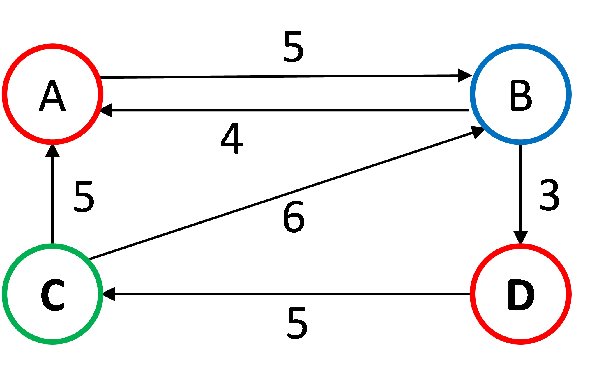
Example 4.1.

ex:objective Consider a small traffic network of four pickup/dropoff points as shown in Fig. 3, out of which two relocation centers are to be identified. Table 1 give the shortest travel time with and without the weighted by gap $g_{i}$ in destination vertex $v_{i}$ . In Table 2, we give the objective value with different objective. Here $F(\mathcal{C},V)=\operatornamewithlimits{\Sigma}_{i=1}^{n}\operatornamewithlimits{\min}_{c_{j}\in\mathcal{C}}\{d(c_{j},v_{i})\}$ . Then with objective function $F(\mathcal{C},V)$ , the low demand vertex B and no demand vertex C would be the centers. However, with the function $F(C,V,W_{v})$ , the two high demand vertices A and D minimize the function $F(C,V,W_{v})$ and they would be the centers. $\blacksquare$

Table 1. Shortest travel time between any two vertices

	d(j, i)				$d(j,i)g_{i}$
	A	B	C	D	A(+1)	B(-1)	C(0)	D(+1)
A	0	5	13	8	0	-5	0	8
B	4	0	8	3	4	0	0	3
C	5	6	0	9	5	-6	0	9
D	10	11	5	0	10	-11	0	0

Table 2. Objective value with different centers

	AB	AC	AD	BC	BD	CD
$F(C,V)$	11	13	10	7	9	11
$F(C,V,W_{v})$	3	2	-11	7	4	-6

To achieve the considered objective, we develop a dynamic traffic condition and travel demand aware road graph partitioning algorithm, and use it to relocate the idle vehicles. The algorithm is based on the ideas of k-medoids (Jin2010; kaufman2009finding; schubert2019faster; park2009simple). As shown in Algorithm 1, there are three steps to find the relocation centers and subareas. The first step initialises by randomly selecting $k$ nodes from the road graph as relocation centers (as shown in Line 1). The second step uses the selected relocation centers $\mathcal{C}$ as centroids to find the subareas $\mathcal{A}$ and calculate the objective value $O(\mathcal{C})$ (as shown in Line 1-1). To be simple in the algorithm, we use $O(\mathcal{C})$ stands for the objective value which means $O(\mathcal{C})=F(C,V,W_{v})$ . The last step calculates new relocation centers $\mathcal{C^{\prime}}$ based on the subareas $\mathcal{A}$ . If $O(\mathcal{C^{\prime}})<O(\mathcal{C})$ , then second and third steps are repeated until $O(\mathcal{C^{\prime}})>=O(\mathcal{C})$ . Until the objective value does not decrease, we can get the relocation centers $\mathcal{C}$ and subareas $\mathcal{A}$ (as shown in Line 1-1).

Input:

d(\cdot,\cdot)

k

V=\{v_{i}|i\in(1,2,...,n)\}

, {

g_{i}

}

Output:

\mathcal{A}=\{A_{i}|i\in(1,2,...,k)\}

\mathcal{C}=\{c_{i}|i\in(1,2,...,k)\}

I. Randomly select

k

nodes as the relocation centers

\mathcal{C}=\{v_{i}|i\in random(1,n,k)\}

;

4 // Initialize

\mathcal{C}

II. Find the subareas

\mathcal{A}

and calculate the objective function value

O(\mathcal{C})

based on relocation centers

\mathcal{C}

\mathcal{A}=\{A_{j}=\varnothing|j\in(1,2,...,k)\}

;

7 // Initialize

\mathcal{A}

8 for $v_{i}\in V$ do

j=\operatornamewithlimits{\operatorname*{arg\,min}}_{i}d(c_{i},j)S(g_{i})

;

10 // Find nearest

c_{j}

for

v_{i}

A_{j}.add(v_{i})

;

12 // Add

v_{i}

for set

A_{j}

O(\mathcal{C})=\operatornamewithlimits{\Sigma}_{v_{i}\in V}\operatornamewithlimits{\min}_{c_{j}\in\mathcal{C}}d(c_{j},v_{i})S(g_{i})

;

15 // Calculate the objective function value with

\mathcal{C}

III. Search the new relocation center for each subarea, until the objective function does not decrease.

17 while True do

18 for $A_{i}\in\mathcal{A}$ do

c_{i}^{\prime}=\operatorname*{arg\,min}_{v_{i}\in{V}}{\Sigma d(v_{i},j)},j\in A_{i}

;

20 // Search new center

c_{i}^{\prime}

for subarea

A_{i}

O(\mathcal{C^{\prime}})=\operatornamewithlimits{\Sigma}_{v_{i}\in V}\operatornamewithlimits{\min}_{c_{j}\in\mathcal{C^{\prime}}}d(c_{j},v_{i})S(g_{i})

;

23 // Calculate the new objective function value with

\mathcal{C^{\prime}}

flag=O(\mathcal{C^{\prime}})-O(\mathcal{C})

;

25 // calculate the difference between

O(\mathcal{C^{\prime}})

and

O(\mathcal{C})

\mathcal{C}=\mathcal{C^{\prime}}

;

27 // set

\mathcal{C}

\mathcal{C^{\prime}}

28 Repeat step II. to find the subareas

\mathcal{A}

based on

\mathcal{C}

29 if $flag=0$ then

30 break ;

31 // If the objective function value does not decrease, then stop

Algorithm 1 Relocation Center Searching

Our distance metrics are different as compared to the traditional metrics (such as Manhattan distance or euclidean metric). The distance between any two points $v_{i}$ and $v_{j}$ using traditional metrics is always the same in both ways, i.e., from $v_{i}$ to $v_{j}$ $d(v_{i},v_{j})\neq$ from $v_{j}$ to $v_{i}$ $d(v_{j},v_{i})$ .

This is quite natural in a normal scenario of traffic conditions. Furthermore, the added weights on the distance measures make the calculation more complex. With all these calculations we need to ensure the convergence of Algorithm 1 to a minimum. We give the theoretical proof in Lemma LABEL:lem:convergence that Algorithm 1 always converges to a local minimum. To achieve a near optimal global minimum, we can run the algorithm several times with new random initial selections each time. As each run is independent to each other, the calculations of different runs can be completely parallelised easily.