A Topology-Shape-Metrics Framework for
Ortho-Radial Graph Drawing

Abstract

Orthogonal drawings, i.e., embeddings of graphs into grids, are a classic topic in Graph Drawing. Often the goal is to find a drawing that minimizes the number of bends on the edges. A key ingredient for bend minimization algorithms is the existence of an orthogonal representation that allows to describe such drawings purely combinatorially by only listing the angles between the edges around each vertex and the directions of bends on the edges, but neglecting any kind of geometric information such as vertex coordinates or edge lengths.

In this work, we generalize this idea to ortho-radial representations of ortho-radial drawings, which are embeddings into an ortho-radial grid, whose gridlines are concentric circles around the origin and straight-line spokes emanating from the origin but excluding the origin itself. Unlike the orthogonal case, there exist ortho-radial representations that do not admit a corresponding drawing, for example so-called strictly monotone cycles. An ortho-radial drawing is called valid if it does not contain a strictly monotone cycle. Our first main result is that an ortho-radial representation admits a corresponding drawing if and only if it is valid. Previously such a characterization was only known for ortho-radial drawings of paths, cycles, and theta graphs [23], and in the special case of rectangular drawings of cubic graphs [22], where the contour of each face is required to be a rectangle. Additionally, we give a quadratic-time algorithm that tests for a given ortho-radial representation whether it is valid, and we show how to draw a valid ortho-radial representation in the same running time.

Altogether, this reduces the problem of computing a minimum-bend ortho-radial drawing to the task of computing a valid ortho-radial representation with the minimum number of bends, and hence establishes an ortho-radial analogue of the topology-shape-metrics framework for planar orthogonal drawings by Tamassia [31].

1 Introduction

Grid drawings of graphs embed graphs into grids such that vertices map to grid points and edges map to internally disjoint curves on the grid lines that connect their endpoints. Orthogonal grids, whose grid lines are horizontal and vertical lines, are popular and widely used in graph drawing. Among other applications, orthogonal graph drawings are used in VLSI design (e.g., [34, 4]), diagrams (e.g., [2, 21, 13, 36]), and network layouts (e.g., [30, 25]). They have been extensively studied with respect to their construction and properties (e.g., [33, 5, 6, 29, 1]). Moreover, they have been generalized to arbitrary planar graphs with degree higher than four (e.g., [32, 18, 7]).

(a) Ortho-radial grid.

(b) Cylinder drawing.

Figure 1: An ortho-radial drawing of a graph on a grid (1(a)) and its equivalent interpretation as an orthogonal drawing on a cylinder (1(b)).

Figure 2: Metro map of Berlin using an ortho-radial layout. Image copyright by Maxwell J. Roberts. Reproduced with permission.

Ortho-radial drawings are a generalization of orthogonal drawings to grids that are formed by concentric circles around the origin and straight-line spokes from the origin, but excluding the origin. Equivalently, they can be viewed as graphs drawn in an orthogonal fashion on the surface of a standing cylinder, see Figure 2, or a sphere without the poles. Hence, they naturally bring orthogonal graph drawings to the third dimension.

Among other applications, ortho-radial drawings are used to visualize network maps; see Figure 2. Especially, for metro systems of metropolitan areas they are highly suitable. Their inherent structure emphasizes the city center, the metro lines that run in circles as well as the metro lines that lead to suburban areas. While the automatic creation of metro maps has been extensively studied for other layout styles (e.g., [24, 28, 35, 16]), this is a new and wide research field for ortho-radial drawings [17].

Adapting existing techniques and objectives from orthogonal graph drawings is a promising step to open up that field. One main objective in orthogonal graph drawing is to minimize the number of bends on the edges. The key ingredient of a large fraction of the algorithmic work on this problem is the orthogonal representation, introduced by Tamassia [31], which describes orthogonal drawings by listing (i) the angles formed by consecutive edges around each vertex and (ii) the directions of bends along the edges. Such a representation is valid if (I) the angles around each vertex sum to $360\degree$, and (II) the sum of the angles around each face with $k$ vertices is $(k-2)\cdot 180\degree$ for internal faces and $(k+2)\cdot 180\degree$ for the outer face. The necessity of the first condition is obvious and the necessity of the latter follows from the sum of inner/outer angles of any polygon with $k$ corners. It is thus clear that any orthogonal drawing yields a valid orthogonal representation, and Tamassia [31] showed that the converse holds true as well; for a valid orthogonal representation there exists a corresponding orthogonal drawing that realizes this representation. Moreover, the proof is constructive and allows the efficient construction of such a drawing, a process that is referred to as compaction.

Altogether, this enables a three-step approach for computing orthogonal drawings, the so-called Topology-Shape-Metrics Framework, which works as follows. First, fix a topology, i.e., a combinatorial embedding of the graph in the plane (possibly planarizing it if it is non-planar); second, determine the shape of the drawing by constructing a valid orthogonal representation with few bends; and finally, compactify the orthogonal representation by assigning suitable vertex coordinates and edge lengths (metrics). As mentioned before, this reduces the problem of computing an orthogonal drawing of a planar graph with a fixed embedding to the purely combinatorial problem of finding a valid orthogonal representation, preferably with few bends. The task of actually creating a corresponding drawing in polynomial time is then taken over by the framework. It is this approach that is at the heart of a large body of literature on bend minimization algorithms for orthogonal drawings (e.g., [3, 14, 11, 15, 8, 9, 10]).

Contribution and Outline.

In this paper we establish an analogous drawing framework for ortho-radial drawings. To this end, we introduce so-called ortho-radial representations, which give a combinatorial description of ortho-radial drawings, and therefore can be used to substitute orthogonal representations in the Topology-Shape-Metrics Framework.

More precisely, our contributions are as follows. We show that a natural generalization of the validity conditions (I) and (II) above is not sufficient, and introduce a third, less local condition that excludes so-called strictly monotone cycles, which do not admit an ortho-radial drawing. We prove that these three conditions together fully characterize ortho-radial drawings. Before that, characterizations for bend-free ortho-radial drawings were only known for paths, cycles and theta graphs [23]. Further, for the special case that each internal face is a rectangle, a characterization for cubic graphs was known [22].

On the algorithmic side, we show that testing whether a given ortho-radial representation is drawable can be done in $\mathcal{O}(n^{2})$ time, and a corresponding drawing can be obtained in the same running time. While this does not yet directly allow us to compute ortho-radial drawings with few bends, our result paves the way for a purely combinatorial treatment of bend minimization in ortho-radial drawings, thus enabling the same type of tools that have proven highly successful in minimizing bends in orthogonal drawings. Recently, Niedermann and Rutter [27] presented such a tool based on an integer linear programming formulation showing that the topology-shape-metrics framework for ortho-radial drawings is capable of handling real-world networks such as metro systems.

We formally introduce ortho-radial drawings and ortho-radial representations in Section 3, where we also establish basic properties that will be used throughout this paper. Section 5 introduces basic properties of labelings that are used to describe ortho-radial representations. In Sections 6 and 7 we prove that ortho-radial representations are drawable if and only if they are valid. In Section 8 we give a validity test for ortho-radial representations that runs in $\mathcal{O}(n^{2})$ time. Afterwards, in Section 9, we revisit the rectangulation procedure from Section 7 and show that using the techniques from Section 8 it can be implemented to run in $\mathcal{O}(n^{2})$ time, improving over a naive application which would yield running time $\mathcal{O}(n^{4})$. This enables a purely combinatorial treatment of ortho-radial drawings. In Section 10 we show that computing bend-minimal ortho-radial representations is $\mathcal{NP}$-complete regardless of whether the embedding of the graph is fixed or not. We conclude with a summary and some open questions in Section 11.

2 Preliminaries

Let $G$ be a plane graph with combinatorial embedding $\mathcal{E}$ and outer face $f_{o}$. The embedding $\mathcal{E}$ fixes for each vertex $v$ of $G$ the counterclockwise order of the edges incident to $v$ around the vertex $v$. A path in $G$ may contain vertices multiple times, and a cycle $C$ may contain vertices multiple times but may not cross itself in the sense that the pairs of edges along which $C$ enters and leaves a vertex $v$ do not alternate in the cyclic order of edges around $v$ in the embedding $\mathcal{E}$. We consider all paths and cycles to be directed. We represent a path $P$ as the sequence $v_{1}\dots v_{k}$ of its vertices in the order as they appear on $P$. Similarly, we represent a cycle as the sequence $v_{1}\dots v_{k}$ of its vertices in the order as they appear on $C$, where $v_{1}$ is arbitrarily chosen. For any path $P=v_{1}\dots v_{k}$ its reverse is $\mkern 1.5mu\overline{\mkern-1.5muP\mkern-1.5mu}\mkern 1.5mu=v_{k}\dots v_{1}$. The concatenation of two paths $P_{1}$ and $P_{2}$ is written as $P_{1}+P_{2}$. For two edges $uv$ and $wx$ on a path $P$ the subpath from $uv$ to $wx$ is the unique path on $P$ that starts with $uv$ and ends with $wx$, and we denote it by $P[uv,wx]$. If $P$ contains $u$ (or $x$) only once, we may write $u$ instead of $uv$ (or $x$ instead of $wx$). In particular, if $P$ is simple $P[u,x]$ denotes the subpath of $P$ from $u$ to $x$. For a cycle $C$, we similarly denote its reverse by $\mkern 1.5mu\overline{\mkern-1.5muC\mkern-1.5mu}\mkern 1.5mu$, and for edges $uv$ and $wx$ on $C$ the subpath of $C$ from $uv$ to $wx$ in the direction of $C$ is denoted by $C[uv,wx]$.

Moreover, a path or cycle is simple if it contains all vertices at most once. A facial walk $C$ of a face $f$ is a cycle in $G$ that describes the boundary of $f$, i.e., the cycle $C$ consists of edges of $f$ and for any subpath $uvw$ of $C$ the edge $uv$ precedes $vw$ in the cyclic order of edges around $v$ that is defined by $\mathcal{E}$. Any simple cycle $C$ separates two sets of faces. One of these sets contains the outer face $f_{o}$, and we call these faces together with the vertices and edges incident to them the exterior of $C$. Conversely the faces of the other set and their incident vertices and edges form the interior of $C$. Note that $C$ belongs to both its interior and its exterior. Unless specified explicitly, a simple cycle $C$ is directed such that its interior lies to the right of $C$. Finally, a path $P$ respects a cycle $C$ if $P$ lies in the exterior of $C$.

3 Ortho-Radial Drawings and Representations

Let $G=(V,E)$ be a planar, connected 4-graph with $n$ vertices, where a graph is a 4-graph if it has maximum degree four. An ortho-radial drawing $\Delta$ of $G$ is a plane drawing on an ortho-radial grid $\mathcal{G}$ such that each vertex of $G$ is a grid point of $\mathcal{G}$ and each edge of $G$ is a curve on $\mathcal{G}$. We observe that in any ortho-radial drawing there is an unbounded face $f_{o}$ and a face $f_{c}$ that contains the center of the grid; we call the former the outer face and the latter the central face; in our figures we mark the central face using a small “x”. All other faces are regular. We remark that $f_{c}$ and $f_{o}$ are not necessarily distinct. We further distinguish two types of simple cycles. If the central face lies in the interior of a simple cycle, the cycle is essential and otherwise non-essential.

In this paper, we assume that we are given $G$, a fixed combinatorial embedding $\mathcal{E}$ of $G$ and two (not necessarily distinct) faces $f_{c}$ and $f_{o}$ of $\mathcal{E}$. We seek an ortho-radial drawing $\Delta$ of $G$ such that the combinatorial embedding of $\Delta$ is $\mathcal{E}$, the face $f_{c}$ is the central face of $\Delta$ and $f_{o}$ is the outer face of $\Delta$. We call the tuple $I=(G,\mathcal{E},f_{c},f_{o})$ an instance of ortho-radial graph drawing and $\Delta$ a drawing of $I$.

We observe that the definition of ortho-radial drawings allows edges to have bends, i.e., an edge may consist of a sequence of straight-line segments and circular arcs. In this paper, we focus on ortho-radial drawings without bends; we call such drawings bend-free. Hence, each edge is either part of a radial ray or of a concentric circle of $\mathcal{G}$. This is not a restriction as any ortho-radial drawing can be turned into a bend-free drawing by replacing bends with subdivision vertices.

In a bend-free ortho-radial drawing of $G$ each edge has a geometric direction in the sense that is drawn either clockwise, counterclockwise, towards the center or away from the center. Hence, using the metaphor of a cylinder, the edges point right, left, down or up, respectively. Moreover, horizontal edges point left or right, while vertical edges point up or down; see Figure 2.

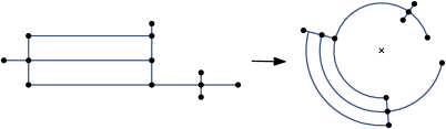
Figure 3: The orthogonal drawing is transformed into an ortho-radial drawing by bending the horizontal edges into concentric circular arcs, while vertical edges become segments of rays that emanate from the center of the ortho-radial grid.

We further observe that if the central and outer face are identical then an ortho-radial drawing can be intepreted as a distorted orthogonal drawing, in which the horizontal edges are bended to circular arcs, while the vertical edges remain straight segments; see Figure 3 for an example. Hence, utilizing the framework for orthogonal drawings by Tamassia [31], this allows us to easily create an ortho-radial drawing of an instance $I$ for the case that the central face $f_{c}$ and the outer face $f_{o}$ are the same. Hence, we assume $f_{c}\neq f_{o}$ in the remainder of this work, which changes the problem of finding an ortho-radial drawing of $I$ substantially.

Figure 4: A combinatorial embedding (left) and a ortho-radial drawing (right) of a graph. For each combinatorial angle a rotation is given.

We first introduce concepts that help us to combinatorially describe the ortho-radial drawing $\Delta$. Let $v$ be a vertex of $G$ and let $\mathcal{E}(v)$ be the counterclockwise order of the edges in $\mathcal{E}$ around $v$. A combinatorial angle at $v$ is a pair of edges $(e_{1},e_{2})$ that are both incident to $v$ and such that $e_{1}$ immediately precedes $e_{2}$ in $\mathcal{E}(v)$; see Figure 4. An angle assignment $\Gamma$ of an instance $I=(G,\mathcal{E},f_{c},f_{o})$ assigns to each combinatorial angle $(e_{1},e_{2})$ of $\mathcal{E}$ a rotation $\operatorname{rot}(e_{1},e_{2})\in\{-2,-1,0,1\}$. For an ortho-radial drawing $\Delta$ of $I$ we can derive an angle assignment that defines $\operatorname{rot}(e_{1},e_{2})=2-2\alpha/\pi$ for each angle $(e_{1},e_{2})$ at $v$, where $\alpha$ is the counterclockwise geometric angle between $e_{1}$ and $e_{2}$ in $\Delta$. Hence, the rotation of a combinatorial angle counts the number of right turns that are taken when going from $e_{1}$ to $e_{2}$ via $v$, where negative numbers correspond to left turns; see Figure 4. In particular, in case that $e_{1}=e_{2}$ we derive $\operatorname{rot}(e_{1},e_{2})=-2$ from $\Delta$, i.e., $v$ contributes two left turns. But conversely, we cannot derive an ortho-radial drawing from every angle assignment.

For a face $f$ of $\mathcal{E}$ with facial walk $v_{1}\dots v_{k}$ around $f$ (where $f$ is oriented in clockwise order) we define $\operatorname{rot}(f)=\sum_{i=1}^{k}\operatorname{rot}(v_{i-1}v_{i},v_{i}v_{i+1})$, where we define $v_{0}:=v_{k}$ and $v_{k+1}:=v_{1}$. Every angle assignment $\Gamma$ that is derived from a bend-free ortho-radial drawing is locally consistent in the following sense [23].

Definition 1.

An angle assignment is locally consistent if it satisfies the following two conditions.

1. For each vertex, the sum of the rotations around $v$ is $2(\deg(v)-2)$.

2. For each face $f$, we have

   $$\operatorname{rot}(f)=\begin{cases}4,&\text{$f$ is a regular face}\\ 0,&\text{$f$ is the outer or the central face but not both}\\ -4,&\text{$f$ is both the outer and the central face.}\\ \end{cases}$$

Figure 5: In this drawing, the angles around vertices sum up to $360^{\circ}$, and also the sum of angles for each face is as expected for an ortho-radial drawing. However, the graph does not have an ortho-radial drawing without bends.

We call a locally consistent angle assignment of $I$ an ortho-radial representation of $I$. Unlike for orthogonal representations Condition (1) and Condition (2) do not guarantee that for an ortho-radial representation of $I$ there is an ortho-radial drawing of $I$ having the same angles; see Figure 5. In this paper, we introduce a third more global condition that characterizes all ortho-radial representations of $I$ that can be drawn. To that end, we first introduce basic concepts on rotations and directions in ortho-radial representations in Section 3.1, which we then use to define this global condition in Section 3.2.

3.1 Rotations and Directions in Ortho-Radial Representations

We transfer two basic properties of ortho-radial drawings to ortho-radial representations. First, the rotations of all cycles are either $0$ or $4$. Second, fixing the geometric direction of a single edge $e^{\star}$, fixes the geometric directions of all edges. We call $e^{\star}$ a reference edge and assume that it points to the right and lies on the outer face of $\mathcal{E}$.

For two edges $e=uv$ and $e^{\prime}=vw$ we define the rotation between them as $\operatorname{rot}(uvw)=\sum_{i=1}^{k-1}\operatorname{rot}(e_{i},e_{i+1})-2(k-2)$, where $e=e_{1},\dots,e_{k}=e^{\prime}$ are the edges that are incident to $v$ and lie between $e$ and $e^{\prime}$ in counterclockwise order; see Figure 6(a).

(a)

(b)

Figure 6: Generalizaton of rotations. (a) The rotation of the two edges $e_{1}=uv$ and $e_{2}=vw$ is $\operatorname{rot}(uvw)=\sum_{i=1}^{3}1-2(4-2)=-1$. (b) The rotation of the path $P$ is $\operatorname{rot}(P)=-1+1-1-1+1+1=0$.

The rotation of a path $P=v_{1}\dots v_{k}$ is the sum of the rotations at its internal vertices, that is $\operatorname{rot}(P)=\sum_{i=2}^{k-1}\operatorname{rot}(v_{i-1}v_{i}v_{i+1})$; see Figure 6(b).

Observation 1.

Let $P$ be a path with start vertex $s$ and end vertex $t$.

1. It is $\operatorname{rot}(\mkern 1.5mu\overline{\mkern-1.5muP\mkern-1.5mu}\mkern 1.5mu)=-\operatorname{rot}(P)$.

2. For every edge $e$ on $P$ it is $\operatorname{rot}(P)=\operatorname{rot}(P[s,e])+\operatorname{rot}(P[e,t])$.

Similarly, for a cycle $C=v_{1}\ldots v_{k}$, its rotation is the sum of the rotations at all its vertices (where we define $v_{0}=v_{k}$ and $v_{k+1}=v_{1}$), i.e., $\operatorname{rot}(C)=\sum_{i=1}^{k}\operatorname{rot}(v_{i-1}v_{i}v_{i+1})$. We observe that the rotation of a face $f$ is equal to the rotation of the cycle that we obtain from the facial walk around $f$.

Figure 7: Illustration of proof for Lemma 1. The rotation $\operatorname{rot}(abc)$ (orange) is equal to the rotation $\operatorname{rot}(abd)+\operatorname{rot}(dbc)-2$ (blue) for the cases that $d\neq a,c$.

(a) Rule 1

(b) Rule 2

Figure 8: Illustration of the rules introduced in proof for Lemma 1. (8(a)) The degree-1 vertex $u$ is removed. (8(a)) The edge $uv$ separating the faces $f$ and $g$ is removed.

Lemma 1.

Let $C$ be a simple cycle in an ortho-radial representation $\Gamma$. Then, $\operatorname{rot}(C)=0$ if $C$ is essential and $\operatorname{rot}(C)=4$ if $C$ is non-essential.

Proof.

Let $H$ be the sub-graph of $G$ that is contained in the interior of $C$; we note that $C$ belongs to $H$. We remove $H^{\circ}=H-C$ from the ortho-radial representation by deleting the edges and vertices of $H^{\circ}$ successively. We show that in each deletion step we again obtain an ortho-radial representation; in particular Condition 1 and Condition 2 hold. After $H^{\circ}$ has been completely removed, the cycle $C$ is a face of the resulting ortho-radial representation. By Condition 2 the statement follows.

We do the removal of $H^{\circ}$ based on two rules. The first rule removes a degree-1 vertex from $H^{\circ}$ adapting the angle assignment accordingly. The second rule removes an edge of $H^{\circ}$ that lies on a cycle of $H$ adapting the angle assignment accordingly.

We show the following claims.

Claim 1: If $H^{\circ}$ is not empty, then the first or second rule is applicable.

Claim 2: Applying the first rule yields a connected graph and an ortho-radial representation of this graph.

Claim 3: Applying the second rule yields a connected graph and an ortho-radial representation of this graph.

We now prove Claim 3.1. Assume that the second rule is not applicable, but $H^{\circ}$ contains at least one vertex. We contract $C$ and the sub-graph in the exterior of $C$ to one vertex. As the second rule is not applicable, the result is a tree, which shows that there is a degree-1 vertex in $H^{\circ}$. Hence, the first rule is applicable.

For proving Claim 3.1 and Claim 3.1 we first show a general statement on rotations. Let $a$, $b$, $c$ and $d$ vertices of $G$ such that $d\neq c,a$ and there are the edges $ab$, $bc$ and $bd$. We assume that $ab$, $bc$ and $bd$ appear around $b$ in clockwise order. Figure 7 shows the six cases that are possible, from which we derive

$$\operatorname{rot}(abc)=\operatorname{rot}(abd)+\operatorname{rot}(dbc)-2$$ (1)

We now prove Claim 3.1. Let $u$ be a degree-1 vertex and let $v$ be the adjacent vertex of $u$; see Figure 8(a). The edge $uv$ lies on a face $f$. Let $xv$ and $vw$ be the preceding and succeeding edges of $uv$ on $f$, respectively. We note that, possibly, $x=w$. Let $h$ be the new face after deleting $v$. As $u$ has degree one, the resulting graph after deleting $u$ is still connected. Further, we define the deletion of $u$ such that the resulting angle assignment is locally correct, i.e., such that it satisfies Condition 1 at $v$. In order to prove Condition 2 we apply Equation (1) with $a=x$, $b=v$, $c=w$ and $d=u$ as follows.

$$\operatorname{rot}(f)=\operatorname{rot}(f[vw,xv])+\operatorname{rot}(xvu)-2+\operatorname{rot}(uvw)=\operatorname{rot}(f[vw,xv])+\operatorname{rot}(xvw)=\operatorname{rot}(h)$$

If $f$ is a regular face, then $h$ is also a regular face. Hence, we obtain $\operatorname{rot}(h)=4$. If $f$ is the central face, then $h$ is also the central face so that $\operatorname{rot}(h)=0$.

Finally, we prove Claim 3.1. Let $uv$ be the edge that is removed; see Figure 8(b). As $uv$ lies on a cycle in $H$, it separates two faces $f$ and $g$. We assume that $f$ lies locally to the left of $uv$ and $g$ lies locally to the right of $uv$. Let $w$ and $x$ be the preceding and succeeding vertex on $f$, respectively. Further, let $y$ and $z$ be the preceding and succeeding vertex on $g$. We note that possibly  $w=z$ or $x=y$. Let $h$ be the new face after deleting $uv$, whose boundary consists of the two paths $f[ux,wv]$ and $g[vz,yu]$. As $uv$ lies on a cycle, the resulting graph after deleting $uv$ is still connected. Further, we define the deletion of $uv$ such that the resulting angle assignment is locally correct, i.e., such that it satisfies Condition 1 at $u$ and $v$. We prove Condition 2 by showing

$$\operatorname{rot}(h)=\operatorname{rot}(f)+\operatorname{rot}(g)-4.$$ (2)

Since $f$ and $g$ lie in the interior of the essential cycle $C$, neither $f$ nor $g$ is the outer face. If both are regular faces, then $h$ is also regular. From Equation (2) we correctly obtain $\operatorname{rot}(h)=4$. If one of them is the central face, then $h$ is the new central face. From Equation (2) we obtain $\operatorname{rot}(h)=0$. In the remainder of the proof we show $\operatorname{rot}(h)=\operatorname{rot}(f)+\operatorname{rot}(g)-4$. For $f$, $g$ and $h$ we obtain the following rotations.

$$\operatorname{rot}(f) =\operatorname{rot}(f[ux,wv])+\operatorname{rot}(wvu)+\operatorname{rot}(vux)$$

$$\operatorname{rot}(g) =\operatorname{rot}(g[vz,yu])+\operatorname{rot}(yuv)+\operatorname{rot}(uvz)$$

$$\operatorname{rot}(h) =\operatorname{rot}(f[ux,wv])+\operatorname{rot}(wvz)+\operatorname{rot}(g[vz,yu])+\operatorname{rot}(yux)$$

Replacing $\operatorname{rot}(f[ux,wv])$ and $\operatorname{rot}(g[vz,yu])$ in the last equation, we obtain the next equation.

$$\operatorname{rot}(h)= \operatorname{rot}(f)-\operatorname{rot}(wvu)-\operatorname{rot}(vux)+\operatorname{rot}(wvz)+$$

$$\operatorname{rot}(g)-\operatorname{rot}(yuv)-\operatorname{rot}(uvz)+\operatorname{rot}(yux)$$

$$= \operatorname{rot}(f)+\operatorname{rot}(wvz)-\operatorname{rot}(wvu)-\operatorname{rot}(uvz)+$$

$$\operatorname{rot}(g)+\operatorname{rot}(yux)-\operatorname{rot}(yuv)-\operatorname{rot}(vux)$$

Applying Equation (1) twice, we replace $\operatorname{rot}(wvz)-\operatorname{rot}(wvu)-\operatorname{rot}(uvz)$ and $\operatorname{rot}(yux)-\operatorname{rot}(yuv)-\operatorname{rot}(vux)$ with $-2$ each, which yields $\operatorname{rot}(h)=\operatorname{rot}(f)+\operatorname{rot}(g)-4$ as desired. ∎∎

Figure 9: Illustration for proof of Lemma 2. Cycle $C$ with two additional edges $ab$ and $cd$. If $a$ lies in the exterior of $C$ then $r_{a}=+2$ and otherwise $r_{a}=-2$. Similarly, if $d$ lies in the exterior of $C$ then $r_{d}=+2$ and $r_{d}=-2$ otherwise.

The next lemma relates the rotations of two paths $S$ and $T$ that use the same edges except on a cycle $C$; see Figure 9.

Lemma 2.

Let $C$ be a cycle and let $ab$ and $cd$ be two edges (with $b\neq c$) such that $b$ and $c$ lie on $C$, but $a$ and $d$ do not. Further, let $S=ab+C[b,c]+cd$ and $T=ab+\mkern 1.5mu\overline{\mkern-1.5muC\mkern-1.5mu}\mkern 1.5mu[b,c]+cd$. Then

$$\operatorname{rot}(S)-\operatorname{rot}(T)=\operatorname{rot}(C)+r_{a}+r_{d}\,,$$

where for $z\in\{a,d\}$ we define $r_{z}=+2$ if $z$ lies in the interior of $C$ and $r_{z}=-2$ if $z$ lies in the exterior of $C$.

Proof.

Figure 10: Illustration for proof of Lemma 2. In all six cases it holds $\operatorname{rot}(abs)-\operatorname{rot}(abt)=\operatorname{rot}(tbs)+r_{a}$

Let $t$ and $s$ be the vertices immediately before and after $b$ on $C$. We observe that $a$ lies in the interior of $C$ if and only if $ab$ lies locally to the right of the path $sbt$. Considering all six cases how the edges $ab$, $sb$, and $tb$ can be arranged (see Figure 10), we obtain $\operatorname{rot}(abs)-\operatorname{rot}(abt)=\operatorname{rot}(tbs)+r_{a}$. Similarly, we define $s^{\prime}$ and $t^{\prime}$ as the vertices immediately before and after $c$ on $C$. Considering all cases as above we get $\operatorname{rot}(s^{\prime}cd)-\operatorname{rot}(t^{\prime}cd)=\operatorname{rot}(s^{\prime}bt^{\prime})+r_{d}$.

Splitting $S$ and $T$ into three parts (see Figure 9), we have

$$\operatorname{rot}(S)-\operatorname{rot}(T) =\operatorname{rot}(abs)+\operatorname{rot}(C[b,c])+\operatorname{rot}(s^{\prime}cd)-\operatorname{rot}(abt)-\operatorname{rot}(\mkern 1.5mu\overline{\mkern-1.5muC\mkern-1.5mu}\mkern 1.5mu[b,c])-\operatorname{rot}(t^{\prime}cd).$$

Combining the rotations at $b$ and $c$ using the observations from above, we get

$$\operatorname{rot}(S)-\operatorname{rot}(T) =\operatorname{rot}(tbs)+r_{a}+\operatorname{rot}(C[b,c])+\operatorname{rot}(C[c,b])+\operatorname{rot}(s^{\prime}ct^{\prime})+r_{d}$$

$$=\operatorname{rot}(C)+r_{a}+r_{d}.$$

∎∎

(a)

(b)

Figure 11: Illustration of the proof for Lemma 3. (11(a)) The edges $e$ and $e^{\prime}$ are replaced by the depicted construction to reduce the number of cases to be considered. (11(b)) Four cases are considered how the edges $e$ and $e^{\prime}$ can be connected by the path $S$. The paths $S_{1}$ and $S_{2}$ are defined depending on the particular case.

For two edges $e$ and $e^{\prime}$ let $P$ be an arbitrary path that starts at the source or target of $e$ and ends at the source or target of $e^{\prime}$, and that neither contains $e$ nor $e^{\prime}$. We call $P$ a reference path from $e$ to $e^{\prime}$. We define the combinatorial direction of $e^{\prime}=xy$ with respect to $e=uv$ and $P$ as

$$\operatorname{dir}(e,P,e^{\prime})=\begin{cases}\operatorname{rot}(e+P+e^{\prime})&\text{$P$ starts at $v$ and ends at $x$},\\ \operatorname{rot}(\mkern 1.5mu\overline{\mkern-1.5mue\mkern-1.5mu}\mkern 1.5mu+P+e^{\prime})+2&\text{$P$ starts at $u$ and ends at $x$},\\ \operatorname{rot}(e+P+\mkern 1.5mu\overline{\mkern-1.5mue^{\prime}\mkern-1.5mu}\mkern 1.5mu)-2&\text{$P$ starts at $v$ and ends at $y$},\\ \operatorname{rot}(\mkern 1.5mu\overline{\mkern-1.5mue\mkern-1.5mu}\mkern 1.5mu+P+\mkern 1.5mu\overline{\mkern-1.5mue^{\prime}\mkern-1.5mu}\mkern 1.5mu)&\text{$P$ starts at $u$ and ends at $y$.}\end{cases}$$

With the fixed direction of the reference edge $e^{\star}$, it is natural to determine the direction of any other edge $e$ by considering the direction of any reference path from $e^{\star}$ to $e$. In order to get consistent results, any two reference paths $P$ and $Q$ from $e^{\star}$ to $e$ must induce the same direction of $e$, which means that $\operatorname{dir}(e^{\star},P,e)$ and $\operatorname{dir}(e^{\star},Q,e)$ may only differ by a multiple of 4. In the following lemma we show that this is indeed the case.

Lemma 3.

Let $e$ and $e^{\prime}$ be two edges of an ortho-radial representation $\Gamma$, and let $P$ and $Q$ be two reference paths from $e$ to $e^{\prime}$.

1. It holds $\operatorname{dir}(e,P,e^{\prime})\equiv\operatorname{dir}(e,Q,e^{\prime})\pmod{4}$.

2. It holds $\operatorname{dir}(e,P,e^{\prime})=\operatorname{dir}(e,Q,e^{\prime})$, if there are two essential cycles $C$ and $C^{\prime}$ such that

   1. $C^{\prime}$ lies in the interior of $C$,

   2. $e$ lies on $C$ and $e^{\prime}$ lies on $C^{\prime}$, and

   3. $P$ and $Q$ lie in the interior of $C$ and in the exterior of $C^{\prime}$.

Proof.

First, we define a construction that helps us to reduce the number of cases to be considered. We subdivide $e$ by a vertex $u$ into two edges $e_{1}$ and $e_{2}$; see Figure 11(a). Further, we add a path consisting of two edges $e_{3}$ and $e_{4}$ such that the target of $e_{4}$ is $u$. We define that $\operatorname{rot}(e_{3}e_{4})=1$ and $\operatorname{rot}(e_{4}e_{2})=-1$. Similarly, we subdivide $e^{\prime}$ by a vertex $v$ into two edges $e^{\prime}_{1}$ and $e^{\prime}_{2}$. Further, we add a path consisting of two edges $e^{\prime}_{3}$ and $e^{\prime}_{4}$ such that the source of $e^{\prime}_{3}$ is $v$. We define that $\operatorname{rot}(e^{\prime}_{1}e^{\prime}_{3})=1$ and $\operatorname{rot}(e^{\prime}_{3}e^{\prime}_{4})=-1$. Let $S$ be a reference path from $e$ to $e^{\prime}$; see Figure 11(b). Let $S_{1}$ be the path that starts at the source of $e_{3}$ and ends at the starting point of $S$ only using edges from $\{e_{1},e_{2},e_{3},e_{4}\}$. Further, let $S_{2}$ be the path that starts at the end point of $S$ and ends at the target of $e^{\prime}_{4}$ only using edges from $\{e^{\prime}_{1},e^{\prime}_{2},e^{\prime}_{3},e^{\prime}_{4}\}$. The extension $S^{\prime}$ of $S$ is the path $S_{1}+S+S_{2}$. The following claim shows that we can consider $S^{\prime}$ instead of $S$ such that it is sufficient to consider the rotation of $S^{\prime}$ instead of the direction $\operatorname{dir}(e,S,e^{\prime})$, which distinguishes four cases.

Claim 1: $\operatorname{dir}(e,S,e^{\prime})=\operatorname{rot}(S^{\prime})$

The detailed proof of Claim 3.1 is found at the end of this proof. In the following let $P^{\prime}$ and $Q^{\prime}$ be the extensions of $P$ and $Q$, respectively. We show that $\operatorname{rot}(P^{\prime})\equiv\operatorname{rot}(Q^{\prime})\pmod{4}$. Moreover, for the case that $e=e^{\star}$ and $e^{\prime}$ lies on an essential cycle that is respected by $P$ and $Q$, we show that $\operatorname{rot}(P^{\prime})=\operatorname{rot}(Q^{\prime})$. Altogether, due to Claim 3.1 this proves Lemma 3. We show $\operatorname{rot}(P^{\prime})=\operatorname{rot}(Q^{\prime})$ by converting $P^{\prime}$ into $Q^{\prime}$ successively. More precisely, we construct paths $R_{1}\dots R_{k}$ such that $R_{i}$ consists of a prefix of $P^{\prime}$ followed by a suffix of $Q^{\prime}$ such that with increasing $i$ the used prefix of $P^{\prime}$ becomes longer, while the used suffix of $Q^{\prime}$ becomes shorter. In particular, we have $R_{1}=Q^{\prime}$ and $R_{k}=P^{\prime}$. We show that $\operatorname{rot}(R_{i})\equiv\operatorname{rot}(R_{i+1})\pmod{4}$. If $R_{i}\neq P^{\prime}$, we construct $R_{i+1}$ from $R_{i}$ as follows; see Figure 12.

Figure 12: Illustration for proof of Lemma 3. The path $R_{i}$ (gray) consists of a prefix of the path $P^{\prime}$ (orange) and a suffix of the path $Q^{\prime}$ (blue).

There is a first edge $vw$ on $P^{\prime}$ such that the following edge does not lie on $R_{i}$. Let $x$ be the first vertex on $P^{\prime}$ after $w$ that lies on $R_{i}$ and let $y$ be the vertex on $R_{i}$ that follows $x$ immediately. As both $P^{\prime}$ and $R_{i}$ end at the same edge, these vertices always exist. We define $R_{i+1}=P[e_{3},x]+R_{i}[x,e_{4}^{\prime}]$. We observe that $R_{i}[x,e_{4}^{\prime}]=Q^{\prime}[x,e_{4}^{\prime}]$, as $R_{i}[w,e_{4}^{\prime}]=Q^{\prime}[w,e_{4}^{\prime}]$ and $x$ occurs on $Q^{\prime}$ after $w$. Further, $R_{i+1}$ is a path as we can argue as follows. We can decompose $R_{i+1}$ into three paths: $R^{1}_{i+1}=P^{\prime}[e_{3},w]=R_{i}[e_{3},w]$, $R^{2}_{i+1}=P^{\prime}[w,x]$ and $R^{3}_{i+1}=Q^{\prime}[x,e_{4}^{\prime}]=R_{i}[x,e_{4}^{\prime}]$. The paths $R^{1}_{i+1}$ and $R^{3}_{i+1}$ do not intersect as both also belong to $R_{i}$, which is a path by induction. The paths $R^{1}_{i+1}$ and $R^{2}_{i+1}$ do not intersect (except at their common vertex $w$), because both belong to $P^{\prime}$. The paths $R^{2}_{i+1}$ and $R^{3}_{i+1}$ do not intersect (except at their common vertex $x$), because by the definition of $x$ no vertex of $P^{\prime}$ between $w$ and $x$ lies on $R_{i}$.

Next, we show that $\operatorname{rot}(R_{i})\equiv\operatorname{rot}(R_{i+1})\pmod{4}$. To that end consider the cycle $C_{i}$ that consists of the two paths $R_{i}[w,x]$ and $R_{i+1}[w,x]$. We orient $C_{i}$ such that the interior of the cycle locally lies to the right of its edges. By the definition of $R_{i+1}$ we obtain $\operatorname{rot}(R_{i}[e_{3},vw])=\operatorname{rot}(R_{i+1}[e_{3},vw])$ and $\operatorname{rot}(R_{i}[xy,e_{4}^{\prime}])=\operatorname{rot}(R_{i+1}[xy,e_{4}^{\prime}])$, as these subpaths of $R_{i}$ and $R_{i+i}$ coincide, respectively. Hence, it remains to show that $\operatorname{rot}(R_{i}[vw,xy])\equiv\operatorname{rot}(R_{i+1}[vw,xy])\pmod{4}$ and $\operatorname{rot}(R_{i}[vw,xy])=\operatorname{rot}(R_{i+1}[vw,xy])$ in the special case that $e=e^{\star}$ and $e^{\prime}$ lies on an essential cycle that is respected by $P$ and $Q$.

In general we can describe the obtained situation as follows. We are given a cycle and two edges $ab$ and $cd$ (with $b\neq c$) such that $b$ and $c$ lie on that cycle, but $a$ and $d$ not; see also Figure 9. Hence, we can apply Lemma 2.

We distinguish two cases: if the interior of $C_{i}$ lies locally to the right of $R_{i}$ we define $S=vw+R_{i}[w,x]+xy$ and $T=vw+R_{i+1}[w,x]+xy$, and otherwise $S=vw+R_{i+1}[w,x]+xy$ and $T=vw+R_{i}[w,x]+xy$. We only consider the first case, as the other case is symmetric. By Lemma 2 we obtain $\operatorname{rot}(S)-\operatorname{rot}(T)=\operatorname{rot}(C_{i})+r_{v}+r_{y}$. As $\operatorname{rot}(C_{i})\equiv 0\pmod{4}$ and $r_{v},r_{y}\equiv 2\pmod{4}$ we obtain $\operatorname{rot}(S)\equiv\operatorname{rot}(T)\pmod{4}$ and with this $\operatorname{rot}(R_{i}[vw,xy])\equiv\operatorname{rot}(R_{i+1}[vw,xy])\pmod{4}$. Altogether, in the general case we obtain $\operatorname{rot}(R_{i})\equiv\operatorname{rot}(R_{i+1})$.

Finally, we prove the second statement of the lemma. Hence, there are two essential cycles $C$ and $C^{\prime}$ such that

1. $C^{\prime}$ lies in the interior of $C$,

2. $e$ lies on $C$ and $e^{\prime}$ lies on $C^{\prime}$, and

3. $P$ and $Q$ lie in the interior of $C$ and in the exterior of $C^{\prime}$.

In particular, the paths $P$ and $Q$ respect $C^{\prime}$ as they lie in the exterior of $C^{\prime}$. We show that $\operatorname{rot}(S)=\operatorname{rot}(T)$. First, we observe that $R_{i}[e,vw]$ respects the cycle $C_{i}$ by the simplicity of $R_{i}$ and $R_{i+1}$. In particular, $vw$ lies in the exterior of $C_{i}$ so that $r_{v}=-2$. We distinguish the two cases whether $C_{i}$ is essential or non-essential. If $C_{i}$ is a non-essential cycle, the edge $xy$ is also contained in the exterior of $C_{i}$ as $P$ and $Q$ end on the essential cycle $C^{\prime}$, which both respect. Hence, we obtain $r_{y}=-2$. Thus, we get by Lemmas 1 and 2 that $\operatorname{rot}(S)-\operatorname{rot}(T)=\operatorname{rot}(C_{i})+r_{v}+r_{y}=4-2-2=0$. If $C_{i}$ is an essential cycle, then the cycle $C^{\prime}$ is contained in the interior of $C_{i}$ as both contain the central face, and $C_{i}$ is composed by parts of paths that respect $C^{\prime}$. Consequently, the edge $xy$ lies in the interior of $C_{i}$ so that we obtain $r_{y}=2$. By Lemmas 1 and 2 we get $\operatorname{rot}(S)-\operatorname{rot}(T)=\operatorname{rot}(C_{i})+r_{v}+r_{y}=0-2+2=0$. It remains to prove Claim 3.1.

Proof of Claim 3.1. We distinguish the four cases given by the definition of $\operatorname{dir}(e,S,e^{\prime})$; see Figure 11(b). If $S$ starts at the target of $e$ and ends at the source of $e^{\prime}$, we obtain $\operatorname{dir}(e,S,e^{\prime})=\operatorname{rot}(e+S+e^{\prime})=\operatorname{rot}(e_{2}+S+e^{\prime}_{1})$ as subdividing $e$ and $e^{\prime}$ transfers the directions of $e$ and $e^{\prime}$ to $e_{2}$ and $e^{\prime}_{1}$, respectively. Hence, we obtain

$$\operatorname{rot}(S^{\prime}) =\operatorname{rot}(S_{1}+S+S_{2})$$

$$=\operatorname{rot}(e_{3}+e_{4}+e_{2}+S+e^{\prime}_{1}+e^{\prime}_{3}+e^{\prime}_{4})$$

$$=\operatorname{rot}(e_{3}+e_{4}+e_{2})+\operatorname{rot}(e_{2}+S+e^{\prime}_{1})+\operatorname{rot}(e^{\prime}_{1}+e^{\prime}_{3}+e^{\prime}_{4})$$

$$=0+\operatorname{dir}(e,S,e^{\prime})+0=\operatorname{dir}(e,S,e^{\prime}).$$

If $S$ starts at the source of $e$ and ends at the source of $e^{\prime}$, we obtain $\operatorname{dir}(e,S,e^{\prime})=\operatorname{rot}(\mkern 1.5mu\overline{\mkern-1.5mue\mkern-1.5mu}\mkern 1.5mu+S+e^{\prime})+2=\operatorname{rot}(\mkern 1.5mu\overline{\mkern-1.5mue_{1}\mkern-1.5mu}\mkern 1.5mu+S+e^{\prime}_{1})+2$ and with this we obtain

$$\operatorname{rot}(S^{\prime}) =\operatorname{rot}(S_{1}+S+S_{2})$$

$$=\operatorname{rot}(e_{3}+e_{4}+\mkern 1.5mu\overline{\mkern-1.5mue_{1}\mkern-1.5mu}\mkern 1.5mu+S+e^{\prime}_{1}+e^{\prime}_{3}+e^{\prime}_{4})$$

$$=\operatorname{rot}(e_{3}+e_{4}+\mkern 1.5mu\overline{\mkern-1.5mue_{1}\mkern-1.5mu}\mkern 1.5mu)+\operatorname{rot}(\mkern 1.5mu\overline{\mkern-1.5mue_{1}\mkern-1.5mu}\mkern 1.5mu+S+e^{\prime}_{1})+\operatorname{rot}(e^{\prime}_{1}+e^{\prime}_{3}+e^{\prime}_{4})$$

$$=2+\operatorname{dir}(e,S,e^{\prime})-2+0=\operatorname{dir}(e,S,e^{\prime}).$$

If $S$ starts at the target of $e$ and ends at the target of $e^{\prime}$, we obtain $\operatorname{dir}(e,S,e^{\prime})=\operatorname{rot}(e+S+\mkern 1.5mu\overline{\mkern-1.5mue^{\prime}\mkern-1.5mu}\mkern 1.5mu)-2=\operatorname{rot}(e_{2}+S+\mkern 1.5mu\overline{\mkern-1.5mue^{\prime}_{2}\mkern-1.5mu}\mkern 1.5mu)-2$ and with this we obtain

$$\operatorname{rot}(S^{\prime}) =\operatorname{rot}(S_{1}+S+S_{2})$$

$$=\operatorname{rot}(e_{3}+e_{4}+e_{2}+S+\mkern 1.5mu\overline{\mkern-1.5mue^{\prime}_{2}\mkern-1.5mu}\mkern 1.5mu+e^{\prime}_{3}+e^{\prime}_{4})$$

$$=\operatorname{rot}(e_{3}+e_{4}+e_{2})+\operatorname{rot}(e_{2}+S+\mkern 1.5mu\overline{\mkern-1.5mue^{\prime}_{2}\mkern-1.5mu}\mkern 1.5mu)+\operatorname{rot}(\mkern 1.5mu\overline{\mkern-1.5mue^{\prime}_{2}\mkern-1.5mu}\mkern 1.5mu+e^{\prime}_{3}+e^{\prime}_{4})$$

$$=0+\operatorname{dir}(e,S,e^{\prime})+2-2=\operatorname{dir}(e,S,e^{\prime}).$$

If $S$ starts at the source of $e$ and ends at the target of $e^{\prime}$, we obtain $\operatorname{dir}(e,S,e^{\prime})=\operatorname{rot}(\mkern 1.5mu\overline{\mkern-1.5mue\mkern-1.5mu}\mkern 1.5mu+S+\mkern 1.5mu\overline{\mkern-1.5mue^{\prime}\mkern-1.5mu}\mkern 1.5mu)=\operatorname{rot}(\mkern 1.5mu\overline{\mkern-1.5mue_{1}\mkern-1.5mu}\mkern 1.5mu+S+\mkern 1.5mu\overline{\mkern-1.5mue^{\prime}_{2}\mkern-1.5mu}\mkern 1.5mu)$ and with this we obtain

$$\operatorname{rot}(S^{\prime}) =\operatorname{rot}(S_{1}+S+S_{2})$$

$$=\operatorname{rot}(e_{3}+e_{4}+\mkern 1.5mu\overline{\mkern-1.5mue_{1}\mkern-1.5mu}\mkern 1.5mu+S+\mkern 1.5mu\overline{\mkern-1.5mue^{\prime}_{2}\mkern-1.5mu}\mkern 1.5mu+e^{\prime}_{3}+e^{\prime}_{4})$$

$$=\operatorname{rot}(e_{3}+e_{4}+\mkern 1.5mu\overline{\mkern-1.5mue_{1}\mkern-1.5mu}\mkern 1.5mu)+\operatorname{rot}(\mkern 1.5mu\overline{\mkern-1.5mue_{1}\mkern-1.5mu}\mkern 1.5mu+S+\mkern 1.5mu\overline{\mkern-1.5mue^{\prime}_{2}\mkern-1.5mu}\mkern 1.5mu)+\operatorname{rot}(\mkern 1.5mu\overline{\mkern-1.5mue^{\prime}_{2}\mkern-1.5mu}\mkern 1.5mu+e^{\prime}_{3}+e^{\prime}_{4})$$

$$=2+\operatorname{dir}(e,S,e^{\prime})-2=\operatorname{dir}(e,S,e^{\prime}).$$

Altogether, this shows the claim $\operatorname{dir}(e,S,e^{\prime})=\operatorname{rot}(S^{\prime})$. ∎∎

Corollary 1.

If $e$ is the reference edge $e^{\star}$ and $e^{\prime}$ lies on an essential cycle that is respected by $P$ and $Q$, then $\operatorname{dir}(e,P,e^{\prime})=\operatorname{dir}(e,Q,e^{\prime})$.

Proof.

The statement directly follows from the second statement of Lemma 3 by assuming that $C$ is the outermost essential cycle of $\Gamma$ and $C^{\prime}$ is the cycle containing $e^{\prime}$. ∎∎

Using this result, the geometric directions of all edges of a given ortho-radial representation $\Gamma$ can be determined as follows. Let $P$ be any reference path from the reference edge $e^{\star}$ to any edge $e$, the edge $e$ points right, down, left, and up if $\operatorname{dir}(e^{\star},P,e)$ is congruent to 0, 1, 2, and 3, respectively. Lemma 3 ensures that the result is independent of the choice of the reference path. In fact, Lemma 3 even gives a stronger result as we can infer the geometric direction of one edge from the geometric direction of another edge locally without having to resort to paths to the reference edge. We often implicitly make use of this observation in our proofs.

Figure 13: The outer face of an ortho-radial drawing. All outlying edges are marked blue.

3.2 Drawable Ortho-Radial Representations

In this section we introduce concepts that help us to characterize the ortho-radial representations that have an ortho-radial drawing. To that end, consider an arbitrary bend-free ortho-radial drawing $\Delta$ of a plane 4-graph $G$. As we assume throughout this work that the outer and central face are not the same, there is an essential cycle $C$ that lies on the outer face $f$ of $\Delta$. Let $e$ be a horizontal edge of $C$ that points to the right and that lies on the outermost circle of the ortho-radial grid among all such edges, and let $R_{\Delta}$ be the set of all edges $e^{\prime}$ with $\operatorname{dir}(e,P,e^{\prime})=0$ for any path $P$ on $f$; see Figure 13. We observe that $R_{\Delta}$ is independent of the choice of $e$, because if there are multiple choices for $e$, then all of these edges are contained in $R_{\Delta}$. We call the edges in $R_{\Delta}$ the outlying edges of $\Delta$. Without loss of generality, we require that the reference edge of the according ortho-radial representation $\Gamma$ stems from $R_{\Delta}$; as $R_{\Delta}$ is not empty and all of the edges in $R_{\Delta}$ are possible candidates for being a reference edge, we can always change the reference edge of $\Gamma$ to one of the edges in $R_{\Delta}$. These outlying edges possess the helpful properties that they all lie on the outermost essential cycle, which makes them the ideal choice as reference edges.

An ortho-radial representation $\Gamma$ of a graph $G$ with reference edge $e^{\star}$ is drawable if there exists a bend-free ortho-radial drawing $\Delta$ of $G$ embedded as specified by $\Gamma$ such that the corresponding angles in $\Delta$ and $\Gamma$ are equal and the edge $e^{\star}$ is an outlying edge, i.e., $e^{\star}\in R_{\Delta}$. Unlike for orthogonal representations Condition (1) and Condition (2) do not guarantee that the ortho-radial representation is drawable; see Figure 5. Therefore, we introduce a third condition, which is formulated in terms of labelings of essential cycles.

Let $e$ be an edge on an essential cycle $C$ in $G$ and let $P$ be a reference path from the reference edge $e^{\star}$ to $e$ that respects $C$. We define the label of $e$ on $C$ as $\ell_{C}(e)=\operatorname{dir}(e^{\star},P,e)$. By Corollary 1 the label $\ell_{C}(e)$ of $e$ does not depend on the choice of $P$. We call the set of all labels of an essential cycle its labeling.

We call an essential cycle monotone if either all its labels are non-negative or all its labels are non-positive. A monotone cycle is a decreasing cycle if it has at least one strictly positive label, and it is an increasing cycle if it has at least one strictly negative label. We also refer to increasing and decreasing cycles as strictly monotone. An ortho-radial representation is valid if it contains no strictly monotone cycles. The validity of an ortho-radial representation ensures that on each essential cycle with at least one non-zero label there is at least one edge pointing up and one pointing down.

A main goal of this paper is to show that a graph with a given ortho-radial representation can be drawn if and only if the representation is valid. Further, we show how to test validity of a given representation and how to obtain a bend-free ortho-radial drawing from a valid ortho-radial representation in quadratic time. Altogether, this yields our main results:

thmmrDrawable An ortho-radial representation is drawable if and only if it is valid.

thmmrValidity Given an ortho-radial representation $\Gamma$, it can be determined in $\mathcal{O}(n^{2})$ time whether $\Gamma$ is valid. In the negative case a strictly monotone cycle can be computed in $\mathcal{O}(n^{2})$ time.

thmmrDrawing Given a valid ortho-radial representation, a corresponding drawing can be constructed in $\mathcal{O}(n^{2})$ time.

We prove the three theorems in the given order. Section 4–6 deals with Theorem 3.2. In Section 7 we prove Theorem 3.2. In particular, together with the proof of Theorem 3.2 this already leads to a version of Theorem 3.2, but with a running time of $O(n^{4})$. In Section 9 we show how to achieve $O(n^{2})$ running time proving Theorem 3.2.

4 Transformations of Ortho-Radial Representations

In this section we introduce helpful tools that we use throughout this work. In the remainder of this work we assume that we are given an ortho-radial representation $\Gamma$ with reference edge $e^{\star}$.

Since the reference edge lies on an essential cycle by definition, we can compute the labelings of essential cycles via the rotation of paths as shown in the following lemma. This simplifies the arguments of our proofs.

(a)

(b)

Figure 14: Illustration of proof for Lemma 4. The outermost cycle $C^{\prime}$ contains the essential cycle $C$. There is always a reference path from $s$ on $C^{\prime}$ to $t$ on $C$ respecting $C$. (14(a)) The cycles $C$ and $C^{\prime}$ have vertices in common. (14(b)) The cycles $C$ and $C^{\prime}$ are disjoint.

Lemma 4.

For every edge $e$ on an essential cycle $C$ there is a reference path $P$ from $e^{\star}$ to $e$ such that $P$ respects $C$, starts at the target of $e^{\star}$ and ends on the source of $e$. Moreover, $\ell_{C}(e)=\operatorname{rot}(e^{\star}+P+e)$.

Proof.

Let $Q$ be a reference path from the reference edge $e^{\star}=rs$ to $e=tu$ respecting $C$. We construct the desired reference path $P$ as follows. Let $C^{\prime}$ be the outermost essential cycle, i.e., $C^{\prime}$ is the unique essential cycle such that every edge of $C^{\prime}$ bounds the outer face. If $C$ and $C^{\prime}$ have a common vertex, we define $v$ to be the first common vertex on $C^{\prime}$ after $s$; see Figure 14(a). We set $P=C^{\prime}[s,v]+C[v,t]$. By the choice of $v$ this concatenation is a path. Moreover, it is a reference path from $e^{\star}$ to $e$ that respects $C$. If $C$ and $C^{\prime}$ are disjoint, let $v$ be the first vertex of $Q$ lying on $C$ and let $w$ be the last vertex of $Q$ before $v$ that lies on $C^{\prime}$; see Figure 14(b). We set $P=C^{\prime}[s,w]+Q[w,v]+C[v,t]$. We observe that the concatenation $P$ is a path by the choice of $v$ and $w$, and that $P$ is a reference path from $e^{\star}$ to $e$ respecting $C$.

By Corollary 1 we have $\ell_{C}(e)=\operatorname{dir}(e^{\star},P,e)$ since $P$ is a reference path from $e^{\star}$ to $e$ respecting $C$. Further, since $P$ starts at the target $s$ of the reference edge $e^{\star}$ and ends at the source $t$ of the edge $e$, we can express the direction of $P$ as $\operatorname{dir}(e^{\star},P,e)=\operatorname{rot}(e^{\star}+P+e)$. ∎∎

The next lemma shows how we can change the reference edge $e^{\star}$ on the essential cycle $C_{o}$ that is part of the outer face; Figure 15 illustrates the lemma.

(a)

(b)

Figure 15: Illustration of proof for Lemma 5. The outermost cycle $C_{o}$ contains the essential cycle $C$. Further, there is a reference path $P$ from $e^{\star}$ to an edge $e$ on $C$. (14(a)) The path $P$ contains the edge $e^{\star\star}$. (14(b)) The path $P$ does not contain the edge $e^{\star\star}$.

Lemma 5.

Let $\Gamma$ be an ortho-radial representation and let $e^{\star}$ be the reference edge of $\Gamma$. Further, let $C_{o}$ be the essential cycle that lies on the outer face and let $e^{\star\star}$ be an edge on $C_{o}$ such that $\operatorname{rot}(C_{o}[e^{\star},e^{\star\star}])=0$. For every edge $e$ on an essential cycle $C$ of $\Gamma$ it holds $\ell_{C}(e)=\overline{\ell}_{C}(e)$, where $\overline{\ell}_{C}$ is the labeling of $C$ with respect to $e^{\star\star}$.

In particular, $\Gamma$ with reference edge $e^{\star}$ is valid if and only if $\Gamma$ with reference edge $e^{\star\star}$ is valid.

Proof.

Let $e$ be an edge of an essential cycle $C$ in $\Gamma$ and let $P$ be a reference path from $e^{\star}$ to $e$. By Lemma 4 we assume that $P$ starts at the target of $e^{\star}$ and ends at the source of $e$. Without loss of generality we assume that only a prefix of $P$ is part of $C_{o}$. Further, let $e^{\star}=st$ and $e^{\star\star}=s^{\prime}t^{\prime}$.

If $P$ contains $e^{\star\star}$, then

$$\ell_{C}(e)=\operatorname{rot}(e^{\star}+P+e)=\operatorname{rot}(e^{\star}+P[t,e^{\star\star}])+\operatorname{rot}(e^{\star\star}+P^{\prime}+e]),$$

where $P^{\prime}$ is the suffix of $P$ that starts at $t^{\prime}$; see Figure 15(a). By assumption $\operatorname{rot}(e^{\star}+P[t,e^{\star\star}])=0$ and $\overline{\ell}_{C}(e)=\operatorname{rot}(e^{\star\star}+P^{\prime}+e])$.

If $P$ does not contain $e^{\star\star}$, then $C_{o}[t^{\prime},e^{\star}]+P$ is a reference path of $e$ with respect to $e^{\star\star}$, which contains $e^{\star}$; see Figure 15(b). Swapping $e^{\star}$ and $e^{\star\star}$ in the argument of the previous case yields the claim. Note that $\operatorname{rot}(C_{o}[e^{\star\star},e^{\star}])=0$ as $\operatorname{rot}(C_{o})=0$. ∎∎

In our arguments we frequently exploit certain symmetries. For an ortho-radial representation $\Gamma$ we introduce two new ortho-radial representations, its flip $\mathrm{flip}(\Gamma)$ and its mirror $\mathrm{mirror}(\Gamma)$. Geometrically, viewed as a drawing on a cylinder, a flip corresponds to rotating the cylinder by $180\degree$ around a line perpendicular to the axis of the cylinder so that is upside down, see Figure 16, whereas mirroring corresponds to mirroring it at a plane that is parallel to the axis of the cylinder; see Figure 17. Intuitively, the first transformation exchanges left/right and top/bottom, and thus preserves monotonicity of cycles, while the second transformation exchanges left/right but not top/bottom, and thus maps increasing cycles to decreasing ones and vice versa. This intuition indeed holds with the correct definitions of $\mathrm{flip}(\Gamma)$ and $\mathrm{mirror}(\Gamma)$, but due to the non-locality of the validity condition for ortho-radial representations and the dependence on a reference edge this requires some care. The following two lemmas formalize flipped and mirrored ortho-radial representations. We denote the reverse of a directed edge $e$ by $\mkern 1.5mu\overline{\mkern-1.5mue\mkern-1.5mu}\mkern 1.5mu$.

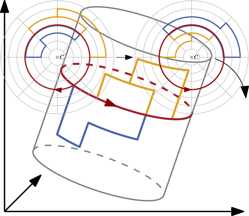
(a) Flipping the cylinder.

(b) The ortho-radial drawing before and after flipping.

Figure 16: Illustration of flipping the cylinder.

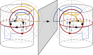
Figure 17: Mirroring the cylinder.

Lemma 6 (Flipping).

Let $\Gamma$ be an ortho-radial representation with outer face $f_{o}$ and central face $f_{c}$. If the cycle bounding the central face is not strictly monotone, there exists an ortho-radial representation $\mathrm{flip}(\Gamma)$ such that

1. $\mkern 1.5mu\overline{\mkern-1.5muf\mkern-1.5mu}\mkern 1.5mu_{c}$ is the outer face of $\mathrm{flip}(\Gamma)$ and $\mkern 1.5mu\overline{\mkern-1.5muf\mkern-1.5mu}\mkern 1.5mu_{o}$ is the central face of $\mathrm{flip}(\Gamma)$,

2. $\mkern 1.5mu\overline{\mkern-1.5mu\ell\mkern-1.5mu}\mkern 1.5mu_{\mkern 1.5mu\overline{\mkern-1.5muC\mkern-1.5mu}\mkern 1.5mu}(\mkern 1.5mu\overline{\mkern-1.5mue\mkern-1.5mu}\mkern 1.5mu)=\ell_{C}(e)$ for all essential cycles $C$ and edges $e$ on $C$, where $\mkern 1.5mu\overline{\mkern-1.5mu\ell\mkern-1.5mu}\mkern 1.5mu$ is the labeling in $\mkern 1.5mu\overline{\mkern-1.5mu\Gamma\mkern-1.5mu}\mkern 1.5mu$.

In particular, increasing and decreasing cycles of $\Gamma$ correspond to increasing and decreasing cycles of $\mathrm{flip}(\Gamma)$, respectively.

Proof.

We define $\mathrm{flip}(\Gamma)$ as follows. The central face of $\Gamma$ becomes the outer face of $\mathrm{flip}(\Gamma)$ and the outer face of $\Gamma$ becomes the central face of $\mathrm{flip}(\Gamma)$. Further, we choose an arbitrary edge $e^{\star\star}$ on the central face $f_{c}$ of $\Gamma$ with $\ell_{f_{c}}(e^{\star\star})=0$ (such an edge exists since the cycle bounding the central face is not strictly monotone), and choose $\mkern 1.5mu\overline{\mkern-1.5mue^{\star\star}\mkern-1.5mu}\mkern 1.5mu$ as the reference edge of $\mathrm{flip}(\Gamma)$. All other information of $\Gamma$ is transferred to $\mathrm{flip}(\Gamma)$ without modification. As the local structure is unchanged, $\mathrm{flip}(\Gamma)$ is an ortho-radial representation.

The essential cycles in $\Gamma$ bijectively correspond to the essential cycles in $\mathrm{flip}(\Gamma)$ by reversing the direction of the cycles. That is, any essential cycle $C$ in $\Gamma$ corresponds to the cycle $\mkern 1.5mu\overline{\mkern-1.5muC\mkern-1.5mu}\mkern 1.5mu$ in $\mathrm{flip}(\Gamma)$. Note that the reversal is necessary since we always consider essential cycles to be directed such that the center lies in its interior, which is defined as the area locally to the right of the cycle.

Consider any essential cycle $C$ in $\Gamma$. We denote the labeling of $C$ in $\Gamma$ by $\ell_{C}$ and the labeling of $\mkern 1.5mu\overline{\mkern-1.5muC\mkern-1.5mu}\mkern 1.5mu$ in $\mathrm{flip}(\Gamma)$ by $\mkern 1.5mu\overline{\mkern-1.5mu\ell\mkern-1.5mu}\mkern 1.5mu_{\mkern 1.5mu\overline{\mkern-1.5muC\mkern-1.5mu}\mkern 1.5mu}$. We show that for any edge $e$ on $C$, $\ell_{C}(e)=\mkern 1.5mu\overline{\mkern-1.5mu\ell\mkern-1.5mu}\mkern 1.5mu_{\mkern 1.5mu\overline{\mkern-1.5muC\mkern-1.5mu}\mkern 1.5mu}(\mkern 1.5mu\overline{\mkern-1.5mue\mkern-1.5mu}\mkern 1.5mu)$, which in particular implies that any monotone cycle in $\Gamma$ corresponds to a monotone cycle in $\mkern 1.5mu\overline{\mkern-1.5mu\Gamma\mkern-1.5mu}\mkern 1.5mu$ and vice versa. By Lemma 4 there is a reference path $P$ from the target of $e^{\star}$ to the source of the edge $e$ respecting $C$. Similarly, there is a path $Q$ from the target of $e$ to the source of $e^{\star\star}$ that lies in the interior of $C$. The path $\mkern 1.5mu\overline{\mkern-1.5muQ\mkern-1.5mu}\mkern 1.5mu$ is a reference path from $e^{\star\star}$ to $\mkern 1.5mu\overline{\mkern-1.5mue\mkern-1.5mu}\mkern 1.5mu$ respecting $\mkern 1.5mu\overline{\mkern-1.5muC\mkern-1.5mu}\mkern 1.5mu$ in $\mathrm{flip}(\Gamma)$.

Assume for now that $P+e+Q$ is simple. We shall see at the end how the proof can be extended if this is not the case. By the choice of $e^{\star\star}$, we have

$$0 =\ell_{f_{c}}(e^{\star\star})=\operatorname{rot}(e^{\star}+P+e+Q+e^{\star\star})=\operatorname{rot}(e^{\star}+P+e)+\operatorname{rot}(e+Q+e^{\star\star})$$ (3)

Hence, $\operatorname{rot}(e^{\star}+P+e)=-\operatorname{rot}(e+Q+e^{\star\star})=\operatorname{rot}(\mkern 1.5mu\overline{\mkern-1.5mue^{\star\star}\mkern-1.5mu}\mkern 1.5mu+\mkern 1.5mu\overline{\mkern-1.5muQ\mkern-1.5mu}\mkern 1.5mu+\mkern 1.5mu\overline{\mkern-1.5mue\mkern-1.5mu}\mkern 1.5mu)$ and in total

$$\mkern 1.5mu\overline{\mkern-1.5mu\ell\mkern-1.5mu}\mkern 1.5mu_{\mkern 1.5mu\overline{\mkern-1.5muC\mkern-1.5mu}\mkern 1.5mu}(\mkern 1.5mu\overline{\mkern-1.5mue\mkern-1.5mu}\mkern 1.5mu)=\operatorname{rot}(\mkern 1.5mu\overline{\mkern-1.5mue^{\star\star}\mkern-1.5mu}\mkern 1.5mu+\mkern 1.5mu\overline{\mkern-1.5muQ\mkern-1.5mu}\mkern 1.5mu+\mkern 1.5mu\overline{\mkern-1.5mue\mkern-1.5mu}\mkern 1.5mu)=\operatorname{rot}(e^{\star}+P+e)=\ell_{C}(e).$$ (4)

Thus, any monotone cycle in $\Gamma$ corresponds to a monotone cycle in $\mathrm{flip}(\Gamma)$ and vice versa.

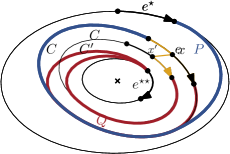
(a)

(b)

Figure 18: Illustration of proof for Lemma 6. (18(a)) The path $P$ is a reference path from $e^{\star}$ to $e$ in $\Gamma$ respecting $C$ and the path $Q$ is a reference path from $e^{\star\star}$ to $\mkern 1.5mu\overline{\mkern-1.5mue\mkern-1.5mu}\mkern 1.5mu$ in $\mathrm{flip}(\Gamma)$ respecting $\mkern 1.5mu\overline{\mkern-1.5muC\mkern-1.5mu}\mkern 1.5mu$. (18(b)) The edge $e$ is subdivided by a vertex $x$. Afterwards, $G$ is cut at $C$ such that the interior and the exterior get their own copies of $C$. The copies are connected by an edge between $x$ and $x^{\prime}$.

If $P+e+Q$ is not simple, we make it simple by cutting $G$ at $C$ such that the interior and the exterior of $C$ get their own copies of $C$; see Figure 18. We connect the two parts by an edge between two new vertices $x$ and $x^{\prime}$ on the two copies of $e$, which we denote by $vw$ in the exterior part and $v^{\prime}w^{\prime}$ in the interior part. The new edge is placed perpendicular to these copies. The path $P+vxx^{\prime}w^{\prime}+Q$ is simple and its rotation is $0$. Hence, the argument above implies $\mkern 1.5mu\overline{\mkern-1.5mu\ell\mkern-1.5mu}\mkern 1.5mu_{\mkern 1.5mu\overline{\mkern-1.5muC\mkern-1.5mu}\mkern 1.5mu}(\mkern 1.5mu\overline{\mkern-1.5mue\mkern-1.5mu}\mkern 1.5mu)=\ell_{C}(e)$. ∎∎

Lemma 7 (Mirroring).

Let $\Gamma$ be an ortho-radial representation with outer face $f_{o}$ and central face $f_{c}$. There exists an ortho-radial representation $\mathrm{mirror}(\Gamma)$ such that

1. $\mkern 1.5mu\overline{\mkern-1.5muf\mkern-1.5mu}\mkern 1.5mu_{o}$ is the outer face of $\mathrm{mirror}(\Gamma)$ and $\mkern 1.5mu\overline{\mkern-1.5muf\mkern-1.5mu}\mkern 1.5mu_{c}$ is the central face of $\mathrm{mirror}(\Gamma)$,

2. $\mathrm{mirror}(\ell)_{\mkern 1.5mu\overline{\mkern-1.5muC\mkern-1.5mu}\mkern 1.5mu}(\mkern 1.5mu\overline{\mkern-1.5mue\mkern-1.5mu}\mkern 1.5mu)=-\ell_{C}(e)$ for all essential cycles $C$ and edges $e$ on $C$, where $\mathrm{mirror}(\ell)$ is the labeling in $\mathrm{mirror}(\Gamma)$.

In particular, increasing and decreasing cycles of $\Gamma$ correspond to decreasing and increasing cycles of $\mathrm{mirror}(\Gamma)$, respectively.

Proof.

We define $\mathrm{mirror}(\Gamma)$ as follows. We reverse the direction of all faces and reverse the order of the edges around each vertex. The outer and central face are equal to those in $\Gamma$ (except for the directions) and the reference edge is $\mkern 1.5mu\overline{\mkern-1.5mue^{\star}\mkern-1.5mu}\mkern 1.5mu$. By this definition $(e_{1},e_{2})$ is a combinatorial angle in $\Gamma$ if and only if $(\mkern 1.5mu\overline{\mkern-1.5mue\mkern-1.5mu}\mkern 1.5mu_{2},\mkern 1.5mu\overline{\mkern-1.5mue\mkern-1.5mu}\mkern 1.5mu_{1})$ is a combinatorial angle in $\mathrm{mirror}(\Gamma)$. We define $\operatorname{rot}_{\mathrm{mirror}(\Gamma)}(\mkern 1.5mu\overline{\mkern-1.5mue\mkern-1.5mu}\mkern 1.5mu_{2},\mkern 1.5mu\overline{\mkern-1.5mue\mkern-1.5mu}\mkern 1.5mu_{1})=\operatorname{rot}_{\Gamma}(e_{1},e_{2})$, where the subscript indicates the ortho-radial representation that defines the rotation. Thus, edges that point left in $\Gamma$ point right in $\mathrm{mirror}(\Gamma)$ and vice versa, but the edges that point up (down) in $\Gamma$ also point up (down) in $\mathrm{mirror}(\Gamma)$. Note that this construction satisfies the conditions for ortho-radial representations.

Let $e=tu$ be an edge on an essential cycle $C$ and let $P$ be a reference path from $e^{\star}=rs$ to $e$ that respects $C$; by Lemma 4 we assume that $P$ starts at $s$ and ends at $t$. After mirroring, $P$ still is a reference path from $e^{\star}$ to $e$, but its rotation in $\mathrm{mirror}(\Gamma)$ may be different from its rotation in $\Gamma$. As above, to distinguish the directions and rotations of paths in $\mathrm{mirror}(\Gamma)$ from the ones in $\Gamma$, we include $\mathrm{mirror}(\Gamma)$ and $\Gamma$ as subscripts to $\operatorname{rot}$ and $\operatorname{dir}$.

As $P$ starts at $s$ and ends at $t$ we have by definition

$$\operatorname{dir}_{\Gamma}(e^{\star},P,e) =\operatorname{rot}_{\Gamma}(e^{\star}+P+e),$$

$$\operatorname{dir}_{\mathrm{mirror}(\Gamma)}(\mkern 1.5mu\overline{\mkern-1.5mue^{\star}\mkern-1.5mu}\mkern 1.5mu,P,\mkern 1.5mu\overline{\mkern-1.5mue\mkern-1.5mu}\mkern 1.5mu) =\operatorname{rot}_{\mathrm{mirror}(\Gamma)}(e^{\star}+P+e).$$

As for any path $Q$ we have $\operatorname{rot}_{\Gamma}(Q)=-\operatorname{rot}_{\mathrm{mirror}(\Gamma)}(Q)$, we obtain $\operatorname{dir}_{\mathrm{mirror}(\Gamma)}(\mkern 1.5mu\overline{\mkern-1.5mue^{\star}\mkern-1.5mu}\mkern 1.5mu,P,\mkern 1.5mu\overline{\mkern-1.5mue\mkern-1.5mu}\mkern 1.5mu)=-\operatorname{dir}_{\Gamma}(e^{\star},P,e)$. By the definition of labels as directions of reference paths we directly obtain that $\mathrm{mirror}(\ell)_{\mkern 1.5mu\overline{\mkern-1.5muC\mkern-1.5mu}\mkern 1.5mu}(\mkern 1.5mu\overline{\mkern-1.5mue\mkern-1.5mu}\mkern 1.5mu)=-\ell_{C}(e)$. In particular, if $C$ is increasing (decreasing) in $\Gamma$, then $\mkern 1.5mu\overline{\mkern-1.5muC\mkern-1.5mu}\mkern 1.5mu$ is decreasing (increasing) in $\mathrm{mirror}(\Gamma)$. ∎∎

5 Properties of Labelings

In this section we study the properties of labelings in more detail to derive useful tools for proving Theorem 3.2. Throughout this section, we are given an instance $(G,\mathcal{E},f_{c},f_{o})$ with an ortho-radial representation $\Gamma$ and a reference edge $e^{\star}$. The following observation follows immediately from the definition of labels and the fact that the rotation of any essential cycle is $0$.

Observation 2.

Let $C$ be an essential cycle. Then, for any two edges $e$ and $e^{\prime}$ on $C$, it holds that $\operatorname{rot}(C[e,e^{\prime}])=\ell_{C}(e^{\prime})-\ell_{C}(e)$.

Note that, if an edge $e$ is contained in two essential cycles $C_{1}$ and $C_{2}$, then their labelings may generally differ, i.e., $\ell_{C_{1}}(e)\neq\ell_{C_{2}}(e)$. In fact, Figure 19 shows that two cycles $C_{1},C_{2}$ may share two edges $e,e^{\prime}$ such that $\ell_{C_{1}}(e)\neq\ell_{C_{2}}(e)$ and $\ell_{C_{1}}(e^{\prime})=\ell_{C_{2}}(e^{\prime})$.

(a)

(b)

Figure 19: (19(a)) Two cycles $C_{1}$ and $C_{2}$ may have both common edges with different labels ($\ell_{C_{1}}(e)=4\neq 0=\ell_{C_{2}}(e)$) and ones with equal labels ($\ell_{C_{1}}(e^{\prime})=\ell_{C_{2}}(e^{\prime})=0$). (19(b)) All labels of $C_{1}[v,w]$ are positive, implying that $C_{1}$ goes down. Note that not all edges of $C_{1}[v,w]$ point downwards.

The rest of this section is devoted to understanding the relationship between labelings of essential cycles that share vertices or edges. The following technical lemma is a key tool in this respect; see also Figure 20.

Figure 20: Illustration of proof for Lemma 8. The essential cycles $C_{1}$ and $C_{2}$ intersect each other having a common vertex $v$. The essential cycle $C$ bounds the central face of $H$.

Lemma 8.

Let $C_{1}$ and $C_{2}$ be two essential cycles and let $H=C_{1}+C_{2}$ be the subgraph of $G$ formed by $C_{1}$ and $C_{2}$. Let $v$ be a common vertex of $C_{1}$ and $C_{2}$ that is incident to the central face of $H$. For $i=1,2$, let further $u_{i}$ and $w_{i}$ be the vertices preceding and succeeding $v$ on $C_{i}$, respectively. Then $\ell_{C_{1}}(vw_{1})=\ell_{C_{1}}(u_{1}v)+\operatorname{rot}(u_{1}vw_{1})=\ell_{C_{2}}(u_{2}v)+\operatorname{rot}(u_{2}vw_{1})$. Moreover, if $w_{1}=w_{2}$, then $\ell_{C_{1}}(vw_{1})=\ell_{C_{2}}(vw_{2})$.

Proof.

Let $C$ be the cycle that bounds the central face of $H$. First assume that the edge $vw_{1}$ is incident to the central face of $H$.

Let $P$ be a reference path from the reference edge to $vw_{1}$ respecting $C_{1}$. Similarly, let $Q$ be a reference path from the reference edge to $vw_{2}$ respecting $C_{2}$. By Lemma 4 we assume that $P$ and $Q$ start at the target of the reference edge and end at $v$. We observe that both $P$ and $Q$ respect the essential cycle $C$.

Then, Corollary 1 applied to $P$ and $Q$ yields

$$\ell_{C}(vw_{1})=\operatorname{rot}(e^{\star}+P+vw_{1})=\operatorname{rot}(e^{\star}+P)+\operatorname{rot}(u_{1}vw_{1})$$

$$\ell_{C}(vw_{1})=\operatorname{rot}(e^{\star}+Q+vw_{1})=\operatorname{rot}(e^{\star}+Q)+\operatorname{rot}(u_{2}vw_{1})$$

By the definition of labelings it is $\ell_{C_{1}}(u_{1}v)=\operatorname{rot}(e^{\star}+P)$, $\ell_{C_{2}}(u_{2}v)=\operatorname{rot}(e^{\star}+Q)$, and $\ell_{C_{1}}(vw_{1})=\ell_{C_{1}}(u_{1}v)+\operatorname{rot}(u_{1}vw_{1})$. Combining this with the previous equation give the desired result:

$$\ell_{C_{1}}(vw_{1})=\ell_{C_{1}}(u_{1}v)+\operatorname{rot}(u_{1}vw_{1})=\ell_{C}(vw_{1})=\ell_{C_{2}}(u_{2}v)+\operatorname{rot}(u_{2}vw_{1}).$$

If $vw_{1}$ does not lie on $C$, then the edge $vw_{2}$ does. By swapping the roles of $C_{1}$ and $C_{2}$ and using the same argument as above, we obtain

$$\ell_{C_{1}}(u_{1}v)+\operatorname{rot}(u_{1}vw_{2})=\ell_{C_{2}}(u_{2}v)+\operatorname{rot}(u_{2}vw_{2}).$$

Since $vw_{1}$ lies locally to the left of both $u_{1}vw_{2}$ and $u_{2}vw_{2}$, it is $\operatorname{rot}(u_{i}vw_{1})=\operatorname{rot}(u_{i}vw_{2})-\alpha$ for $i=1,2$ and the same constant $\alpha$, which is either $1$ or $2$. Hence, we get

$$\ell_{C_{1}}(vw_{1})=\ell_{C_{1}}(u_{1}v)+\operatorname{rot}(u_{1}vw_{1}) =\ell_{C_{1}}(u_{1}v)+\operatorname{rot}(u_{1}vw_{2})-\alpha$$

$$=\ell_{C_{2}}(u_{2}v)+\operatorname{rot}(u_{2}vw_{2})-\alpha=\ell_{C_{2}}(u_{2}v)+\operatorname{rot}(u_{2}vw_{1}).$$

Finally, if $w_{1}=w_{2}$, i.e., $vw_{1}$ lies on both $C_{1}$ and $C_{2}$, then $\ell_{C_{1}}(vw_{1})=\ell_{C_{2}}(u_{2}v)+\operatorname{rot}(u_{2}vw_{1})=\ell_{C_{2}}(u_{2}v)+\operatorname{rot}(u_{2}vw_{2})=\ell_{C_{2}}(vw_{2})$. ∎∎

Corollary 2.

Let $C_{1}$ and $C_{2}$ be two essential cycles, let $H=C_{1}+C_{2}$ be the subgraph of $G$ formed by $C_{1}$ and $C_{2}$, and let $e$ be an edge that lies on both $C_{1}$ and $C_{2}$ and that is incident to the central face of $H$. Then $\ell_{C_{1}}(e)=\ell_{C_{2}}(e)$.

This allows us to prove an important criterion to exclude strictly monotone cycles. We call an essential cycle $C$ horizontal if $\ell_{C}(e)=0$ for all edge $e$ of $C$. We show that a strictly monotone cycle and a horizontal cycle cannot share vertices.

Proposition 1.

Let $C_{2}$ be a horizontal cycle and let $C_{1}$ be an essential cycle that shares at least one vertex with $C_{2}$. Then $C_{1}$ is not strictly monotone.

Figure 21: Illustration of proof for Proposition 1. All edges of $C_{2}$ are labeled with 0. In this situation there are edges on $C_{1}$ with labels $-1$ and $1$. Hence, $C_{2}$ is neither increasing nor decreasing.

Proof.

The situation is illustrated in Figure 21.

If the two cycles are equal, the claim clearly holds. Otherwise, we show that one can find two edges on $C_{1}$ whose labels have opposite signs.

Let $v$ be a shared vertex of $C_{1}$ and $C_{2}$ that is incident to the central face $f$ of $H=C_{1}+C_{2}$ and such that the edge $vw_{1}$ on $C$ is not incident to $f$. For $i=1,2$ denote by $u_{i}$ and $w_{i}$ the vertex preceding and succeeding $v$ on $C_{i}$, respectively. By Lemma 8 it is

$$\ell_{C_{1}}(vw_{1})=\ell_{C_{2}}(u_{2}v)+\operatorname{rot}(u_{2}vw_{1})=\operatorname{rot}(u_{2}vw_{1})\,,$$ (5)

where the second equality follows from the assumption that $\ell_{C_{2}}(u_{2}v)=0$.

Let $y$ be the first common vertex of $C_{1}$ and $C_{2}$ on the central face $f$ after $v$. That is, $f[v,y]$ is a part of one of the cycles $C_{1}$ and $C_{2}$, and it intersects the other cycle only at $v$ and $y$. For $i=1,2$, we denote by $x_{i}$ and $z_{i}$ the vertices preceding and succeeding $y$ on $C_{i}$. Again by Lemma 8 (this time swapping the roles of $C_{1}$ and $C_{2}$), we have

$$0=\ell_{C_{2}}(yz_{2})=\ell_{C_{1}}(x_{1}y)+\operatorname{rot}(x_{1}yz_{2}).$$ (6)

Overall, we have $\ell_{C_{1}}(vw_{1})=\operatorname{rot}(u_{2}vw_{1})$ and $\ell_{C_{1}}(x_{1}y)=-\operatorname{rot}(x_{1}yz_{2})$.

By construction $vw_{1}$ and $x_{1}y$ lie on the same side of $C_{2}$. Hence, $u_{2}vw_{1}$ and $x_{1}yz_{2}$ both make a right turn if $vw_{1}$ and $x_{1}y$ lie in the interior of $C_{2}$ and a left turn otherwise. Thus, it is $\operatorname{rot}(u_{2}vw_{1})=\operatorname{rot}(x_{1}yz_{2})\neq 0$, and therefore $\ell_{C_{1}}(vw_{1})$ and $\ell_{C_{1}}(x_{1}y)$ have opposite signs. Hence, $C_{1}$ is not strictly monotone. ∎∎

In many cases we cannot assume that one of two essential cycles sharing a vertex is horizontal. However, we can still draw conclusions about their intersection behavior from their labelings and find conditions under which shared edges have the same label on both cycles.

Intuitively, positive labels can often be interpreted as going downwards and negative labels as going upwards. In Figure 19(b) all edges of $C_{1}[v,w]$ have positive labels and in total the distance from the center decreases along this path, i.e., the distance of $v$ from the center is greater than the distance of $w$ from the center. Yet, the edges on $C_{1}[v,w]$ point in all possible directions—even upwards. One can still interpret a maximal path with positive labels as leading downwards with the caveat that this is a property of the whole path and does not impose any restriction on the directions of the individual edges.

Using this intuition, we expect that a path $P$ going down cannot intersect a path $Q$ going up if $P$ starts below $Q$. In Lemma 9, we show that this assumption is correct if we restrict ourselves to intersections on the central face.

Lemma 9.

Let $C_{1}$ and $C_{2}$ be two simple, essential cycles in $G$ sharing at least one vertex. Let $H=C_{1}+C_{2}$, and denote the central face of $H$ by $f$. Let $v$ be a vertex that is shared by $C_{1}$ and $C_{2}$ that is incident to $f$ and, for $i=1,2$, let $u_{i}$ and $w_{i}$ be the vertices preceding and succeeding $v$ on $C_{i}$, respectively.

1. If $\ell_{C_{1}}(u_{1}v)\geq 0$ and $\ell_{C_{2}}(u_{2}v)\leq 0$, then $u_{2}v$ lies in the interior of $C_{1}$.

2. If $\ell_{C_{1}}(vw_{1})\geq 0$ and $\ell_{C_{2}}(vw_{2})\leq 0$, then $vw_{2}$ lies in the exterior of $C_{1}$.

(a)

(b)

Figure 22: Possible intersection of two cycles $C$ and $C^{\prime}$ at $v$. (22(a)) The labels of the incoming edges satisfy $\ell_{C_{1}}(u_{1}v)\geq 0$ and $\ell_{C_{2}}(u_{2}v)\leq 0$. The edges $vw_{1}$ and $vw_{2}$ could be exchanged. (22(b)) The labels of the outgoing edges satisfy $\ell_{C_{1}}(vw_{1})\geq 0$ and $\ell_{C_{2}}(vw_{2})\leq 0$. The edges $u_{1}v$ and $u_{2}v$ could be exchanged.

Proof.

The second case follows from the first by taking the mirror representation; this reverses the order on the cycles and changes the sign of each label by Lemma 7, but does not change the notion of interior and exterior. It therefore suffices to consider the first case.

Since the central face $f$ lies in the interior of both $C_{1}$ and $C_{2}$ and $v$ lies on the boundary of $f$, one of the edges $vw_{1}$ and $vw_{2}$ is incident to $f$. We denote this edge by $vx$ and it is either $x=w_{1}$ (as in Figure 22(a)) or $x=w_{2}$. By Lemma 8, we have $\ell_{C_{1}}(u_{1}v)+\operatorname{rot}(u_{1}vx)=\ell_{C_{2}}(u_{2}v)+\operatorname{rot}(u_{2}vx)$. Applying $\ell_{C_{1}}(u_{1}v)\geq 0$ and $\ell_{C_{2}}(u_{2}v)\leq 0$, we obtain $\operatorname{rot}(u_{1}vx)\leq\operatorname{rot}(u_{2}vx)$. Therefore, $u_{2}v$ lies to the right of or on $u_{1}vx$ and thus in the interior of $C_{1}$. ∎∎

The next lemma is a direct consequence of Lemma 9 when applied to decreasing and increasing cycles.

Lemma 10.

A decreasing and an increasing cycle do not have any common vertex.

Figure 23: Illustration of proof for Lemma 10. The cycle $C_{1}$ is increasing and the cycle $C_{2}$ is decreasing. The edge of $C_{2}$ ending at $v$ strictly lies in the exterior of $C_{1}$ and the edge of $C_{2}$ starting at $w$ strictly lies in the interior of $C_{1}$. Hence, the edge of $C_{2}$ ending at $x$ strictly lies in the interior of $C_{1}$, which contradicts Lemma 9.

Proof.

Let $C_{1}$ be an increasing and $C_{2}$ a decreasing cycle. Assume that they have a common vertex. But then there also is a common vertex on the central face $f$ of the subgraph $C_{1}+C_{2}$. Consider any maximal common path $P$ of $C_{1}$ and $C_{2}$ on $f$. We denote the start vertex of $P$ by $v$ and the end vertex by $w$. Note that $v$ may equal $w$. By Lemma 9 the edge to $v$ on the decreasing cycle $C_{2}$ lies strictly in the exterior of $C_{1}$, where the strictness follows from the maximality of $P$. Similarly, the edge from $w$ on $C_{2}$ lies strictly in the interior of $C_{1}$. Hence, $C_{2}[w,v]$ crosses $C_{1}$. Let $x$ be the first intersection of $C_{1}$ and $C_{2}$ on $f$ after $w$. Then the edge to $x$ on $C_{2}$ lies strictly in the interior of $C_{1}$, contradicting Lemma 9. ∎∎

For the correctness proof in Section 7, a crucial insight is that for essential cycles using an edge that is part of a regular face, we can find an alternative cycle without this edge in a way that preserves labels on the common subpath.

Lemma 11.

If an edge $e$ belongs to both a simple essential cycle $C$ and a regular face $f$, then there exists a simple essential cycle $C^{\prime}$ that can be decomposed into two paths $P$ and $Q$ such that

1. $P$ or $\mkern 1.5mu\overline{\mkern-1.5muP\mkern-1.5mu}\mkern 1.5mu$ lies on $f$,

2. $Q=C\cap C^{\prime}$, and

3. $\ell_{C}(e)=\ell_{C^{\prime}}(e)$ for all edges $e$ on $Q$.

(a)

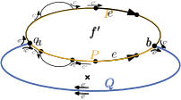
(b)

Figure 24: The edge $e$ cannot lie on both the outer and the central face. In both cases $C^{\prime}$ can be subdivided in two paths $P$ and $Q$ on $C$ and $f$, respectively. Here, these paths are separated by the vertices $a$ and $b$. (24(a)) The cycle bounding the outer face is $C^{\prime}$. The edge $e$ does not lie on the outer face, and hence the cycle bounding this face is defined as $C^{\prime}$. (24(b)) The cycle bounding the central face is $C^{\prime}$.

Proof.

Consider the graph $H=C+f$ composed of the essential cycle $C$ and the regular face $f$. Since $e$ is incident to $f$, the edge $e$ cannot lie on both the outer and the central face in $H$. If $e$ does not lie on the outer face, we define $C^{\prime}$ as the cycle bounding the outer face but directed such that it contains the center in its interior; see Figure 24(a). Otherwise, $C^{\prime}$ denotes the cycle bounding the central face; see Figure 24(b).

Since $C$ lies in the exterior of $f$, the intersection of $C$ with $C^{\prime}$ forms one contiguous path $Q$. Setting $P=C^{\prime}-Q$ yields a path that lies completely on $f$ (it is possible though that $P$ and $f$ are directed differently).

By the construction of $C^{\prime}$ the edges of $Q$ are incident to the central face of $C+C^{\prime}$. Then Lemma 8 implies that $\ell_{C}(e)=\ell_{C^{\prime}}(e)$ for all edges $e$ of $Q$. ∎∎

The last lemma of this section shows that we can replace single edges of an essential cycle $C$ with complex paths without changing the labels of the remaining edges on $C$.

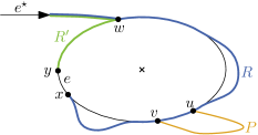
Figure 25: Illustration of the proof for Lemma 12. The reference path $R^{\prime}$ (green) for the edge $xy$ is constructed based on the reference path $R$. Replacing the edge $uv$ with a path $P$, does not impact $R^{\prime}$, which implies that the label of $xy$ remains the same.

Lemma 12.

Let $C$ be an essential cycle in an ortho-radial representation $\Gamma$ and let $uv$ be an edge of $C$. Consider the ortho-radial representation $\Gamma^{\prime}$ that is created by replacing $uv$ with an arbitrary path $P$ such that the interior vertices of $P$ do not belong to $\Gamma$, i.e., they are newly inserted vertices in $\Gamma^{\prime}$. If the cycle $C^{\prime}=C[v,u]+P$ is essential, then the labels of $C$ and $C^{\prime}$ coincide on $C[v,u](=C^{\prime}[v,u])$.

Proof.

For an illustration of the proof see Figure 25. Let $e=xy$ be an arbitrary edge on $C[v,u]$ and let $R$ be a reference path from the reference edge $e^{\star}$ to $e$ that respects $C$. We first construct a new reference path $R^{\prime}$ that does not contain $uv$ as follows. Let $w$ be the first vertex of $R$ that lies on $C$. If $C[w,x]$ does not contain $e$, we define $R^{\prime}=R-R[w,x]+C[w,x]$ and otherwise $R^{\prime}=R-R[w,x]+\mkern 1.5mu\overline{\mkern-1.5muC\mkern-1.5mu}\mkern 1.5mu[w,y]$. We observe that $R^{\prime}$ is again a reference path of $e$ that respects $C$. Further, it can be partitioned into a prefix that only consists of edges that do not belong to $C$ and a suffix that only consists of edges that belong to $C[v,u]$.

We now show that $R^{\prime}$ is a reference path of $e$ in $\Gamma^{\prime}$ that respects $C^{\prime}$. As $R^{\prime}$ does not use $uv$, it is still contained in $\Gamma^{\prime}$ and hence it is a reference path of $e$. So assume that $R^{\prime}$ does not respect $C^{\prime}$. Hence, $R^{\prime}$ and $C^{\prime}$ have a vertex $z$ in common such that the outgoing edge $e^{\prime}$ of $R^{\prime}$ at $z$ strictly lies in the interior of $C^{\prime}$. As $R^{\prime}$ respects $C$, this vertex lies on $P$. It cannot be an intermediate vertex of $P$, because these are newly inserted in $\Gamma^{\prime}$. Hence, $z$ is either $u$ or $v$ and thus part of $C[v,u]$. In particular, it occurs on $R^{\prime}$ after $w$, which implies that $e^{\prime}$ belongs to $C$. This contradicts that $e^{\prime}$ strictly lies in the interior of $C^{\prime}$. Altogether, this shows that $R^{\prime}$ is a reference path of $e$ both in $\Gamma$ and $\Gamma^{\prime}$ such that $C$ and $C^{\prime}$ are respected. Consequently, $\ell_{C}(e)=\ell_{C^{\prime}}(e)$. ∎∎

6 Characterization of Rectangular Ortho-Radial Representations

Throughout this section, assume that $I=(G,\mathcal{E},f_{c},f_{o})$ is an instance with an ortho-radial representation $\Gamma$ and a reference edge $e^{\star}$. We prove Theorem 3.2 for the case that $\Gamma$ is rectangular. In a rectangular ortho-radial representation the central face and the outer face are horizontal cycles, and every regular face is a rectangle, i.e., it has exactly four right turns, but no left turns.

We first observe that a bend-free ortho-radial drawing $\Delta$ can be described by an angle assignment together with the lengths of its vertical edges and the angles of the circular arcs representing the horizontal edges; we call the angles of the circular arcs central angles. We define two flow networks that assign consistent lengths and central angles to the vertical edges and horizontal edges, respectively. These networks are straightforward adaptions of the networks used for drawing rectangular graphs in the plane [12]. In the following, vertex and edge refer to the vertices and edges of $G$, whereas node and arc are used for the flow networks.

(a) $N_{\mathrm{ver}}$

(b) $N_{\mathrm{hor}}$

Figure 26: Flow networks $N_{\mathrm{ver}}$ and $N_{\mathrm{hor}}$ (blue arcs) for an example graph $G$ (black edges).

The network $N_{\mathrm{ver}}=(F_{\mathrm{ver}},A_{\mathrm{ver}})$ with nodes $F_{\mathrm{ver}}$ and arcs $A_{\mathrm{ver}}$ for the vertical edges contains one node for each face of $G$ except for the central and the outer face. All nodes have a demand of 0. For each vertical edge $e$ in $G$, which we assume to be directed upwards, there is an arc $a_{e}=fg$ in $N_{\mathrm{ver}}$, where $f$ is the face to the left of $e$ and $g$ the one to its right. The flow on $fg$ has the lower bound $l(fg)=1$ and upper bound $u(fg)=\infty$. An example of this flow network is shown in Figure 26(a).

Similarly, the network $N_{\mathrm{hor}}=(F_{\mathrm{hor}},A_{\mathrm{hor}})$ assigns the central angles of the horizontal edges. There is a node for each face of $G$, and an arc $a_{e}=fg$ for every horizontal edge $e$ in $G$ such that $f$ lies locally below $e$ and $g$ lies locally above $e$. Additionally, $N_{\mathrm{hor}}$ includes one arc from the outer to the central face. Again, all edges require a minimum flow of 1 and have infinite capacity. The demand of all nodes is 0. Figure 26(b) shows an example of such a flow network. Valid flows in these two flow networks then yield an ortho-radial drawing of $\Gamma$.

Lemma 13.

A pair of valid flows in $N_{\mathrm{hor}}$ and $N_{\mathrm{ver}}$ corresponds to a bend-free ortho-radial drawing of $\Gamma$ and vice versa.

Proof.

Given a feasible flow $\varphi_{\mathrm{ver}}$ in $N_{\mathrm{ver}}$, we set the length of each vertical edge $e$ of $G$ to the flow $\varphi_{\mathrm{ver}}(a_{e})$ on the arc $a_{e}$ that crosses $e$. For each face $f$ of $G$, the total length of its left side is equal to the total amount of flow entering $f$. Similarly, the length of the right side is equal to the amount of flow leaving $f$. As the flow is preserved at all nodes of $N_{\mathrm{ver}}$, the left and right sides of $f$ have the same length. The central angles of the horizontal edges are obtained from a flow $\varphi_{\mathrm{hor}}$ in $N_{\mathrm{hor}}$. Let $\Phi$ be the total amount of flow that leaves the central face. Then for each horizontal edge $e$ we set its central angle to $2\pi\varphi_{\mathrm{hor}}(a_{e})/\Phi$, where $\varphi_{\mathrm{hor}}(a_{e})$ is the amount of flow of the arc $a_{e}$ that connects the two adjacent faces of $e$. As the flow is preserved at all nodes of $N_{\mathrm{hor}}$, the top and bottom sides of each face have the same central angle.

Conversely, given a bend-free ortho-radial drawing $\Delta$ of $\Gamma$, we can extract flows in the two networks. For each vertical edge $e$ we set the flow $\varphi_{\mathrm{ver}}(a_{e})$ of the corresponding arc $a_{e}$ to $l_{e}/l_{\min}$, where $l_{e}$ is the length of $e$ in $\Delta$ and $l_{\min}$ is the length of the shortest edge in $\Delta$. With the scaling, we ensure that the flow of each arc is at least $1$. Similarly, for the horizontal edges we assign to each arc $a_{e}$ of each horizontal edge $e$ the flow $\varphi_{\mathrm{hor}}(a_{e})=\alpha_{e}/\alpha_{\min}$, where $\alpha_{e}$ is the central angle of $e$ in $\Delta$ and $\alpha_{\min}$ is the smallest central angle of any horizontal edge in $\Delta$. Again, the scaling ensures that each arc has flow at least $1$. Since the opposing sides of the regular faces have the same lengths and central angles, the flow is preserved at all nodes. ∎∎

Using this correspondence of drawings and feasible flows, we show the characterization of rectangular graphs.

Theorem 1.

Let $\Gamma$ be a rectangular ortho-radial representation and let $N_{\mathrm{hor}}=(F_{\mathrm{hor}},A_{\mathrm{hor}})$ and $N_{\text{ver}}=(F_{\mathrm{ver}},A_{\mathrm{ver}})$ be the flow networks as defined above. The following statements are equivalent:

1. $\Gamma$ is drawable.

2. $\Gamma$ is valid.

3. For every subset $S\subseteq F_{\mathrm{ver}}$ such that there is an arc from $F_{\mathrm{ver}}\setminus S$ to $S$ in $N_{\mathrm{ver}}$, there is also an arc from $S$ to $F_{\mathrm{ver}}\setminus S$.

Proof.

“(i) $\Rightarrow$ (ii)”: Let $\Delta$ be a bend-free ortho-radial drawing of $G$ preserving the embedding described by $\Gamma$ and let $C$ be an essential cycle. Our goal is to show that $C$ is not strictly monotone. To this end, we construct a path $P$ from the reference edge of $\Gamma$ to a vertex on $C$ such that either the labeling of $C$ induced by $P$ attains both positive and negative values or it is 0 everywhere.

In $\Delta$ either all vertices of $C$ lie on the same concentric circle, or there is a maximal subpath $Q$ of $C$ whose vertices all have maximum distance to the center of the ortho-radial grid among all vertices of $C$. In the first case, we may choose the endpoint $v$ of the path $P$ arbitrarily, whereas in the second case we select the first vertex of $Q$ as $v$; for an example see Figure 27.

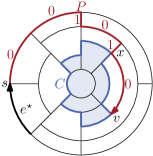
Figure 27: The path $P$ from $s$ to $v$—constructed backwards by going only up or left—does not intersect the interior of $C$. The rotations of the edges on $P$ relative to $e^{\star}$ are 0 or 1.

We construct the path $P$ backwards (i.e., the construction yields $\mkern 1.5mu\overline{\mkern-1.5muP\mkern-1.5mu}\mkern 1.5mu$) as follows: Starting at $v$ we choose the edge going upwards from $v$, if it exists, or the one leading left. Since all faces of $\Gamma$ are rectangles, at least one of these always exists. This procedure is repeated until the target $s$ of the reference edge is reached.

To show that this algorithm terminates, we assume that this was not the case. As $G$ is finite, there must be a first time a vertex $w$ is visited twice. Hence, there is a cycle $C^{\prime}$ in $\Delta$ containing $w$ that contains only edges going left or up. As all drawable essential cycles with edges leading upwards must also have edges that go down [23], all edges of $C^{\prime}$ are horizontal. By construction, there is no edge incident to a vertex of $C^{\prime}$ that leads upwards. The only cycle with this property, however, is the one enclosing the outer face because $G$ is connected. But this cycle contains the reference edge, and therefore the algorithm halts.

This not only shows that the construction of $P$ ends, but also that $P$ is a path (i.e., the construction does not visit a vertex twice). Thus, $P$ is a reference path from the reference edge $e^{\star}$ to the edge $vv^{\prime}$, where $v^{\prime}$ is the vertex following $v$ on $C$. Further, $P$ respects $C$ as $\mkern 1.5mu\overline{\mkern-1.5muP\mkern-1.5mu}\mkern 1.5mu$ starts at the outermost circle of the ortho-radial grid that is used by $C$ and as by construction all edges of $\mkern 1.5mu\overline{\mkern-1.5muP\mkern-1.5mu}\mkern 1.5mu$ point left or upwards.

By the construction of $P$, the label of $vv^{\prime}$ induced by $P$ is $0$. If all edges of $C$ are horizontal, this implies $\ell_{C}(e)=0$ for all edges $e$ of $C$, which shows that $C$ is not strictly monotone. Otherwise, we claim that the edges $e_{-}=uv$ and $e_{+}=wx$ directly before and after $Q$ on $C$ have labels $-1$ and $+1$, respectively. Since all edges on $Q$ are horizontal and $e_{-}$ goes down, we have $\operatorname{rot}(C[v,x])=1$ and therefore $\ell_{C}(e_{+})=1$. Similarly, $\operatorname{rot}(uvv^{\prime})=1$ implies that $\ell_{C}(uv)=\ell_{C}(vv^{\prime})-\operatorname{rot}(uvv^{\prime})=-1$.

“(ii) $\Rightarrow$ (iii)”: Instead of proving this implication directly, we show the contrapositive. That is, we assume that there is a set $S\subsetneq F_{\text{ver}}$ of nodes in $N_{\text{ver}}$ such that $S$ has no outgoing but at least one incoming arc. From this assumption we derive that $\Gamma$ is not valid, as we find a strictly monotone cycle.

Let $N_{\mathrm{ver}}[S]$ denote the node-induced subgraph of $N_{\mathrm{ver}}$ induced by the set $S$. Without loss of generality, $S$ can be chosen such that $N_{\mathrm{ver}}[S]$ is weakly connected, i.e., the underlying undirected graph is connected. If $N_{\mathrm{ver}}$ is not weakly connected, at least one weakly-connected component of $N_{\mathrm{ver}}[S]$ possesses an incoming arc but no outgoing arc, and we can work with this component instead.

As each node of $S$ corresponds to a face of $G$, $S$ can also be considered as a collection of faces of $G$. To distinguish the two interpretations of $S$, we refer to this collection of faces by $\mathcal{S}$. Our goal is to show that the innermost or the outermost boundary of $\mathcal{S}$ forms a strictly monotone cycle in $\Gamma$.

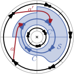
Figure 28: A set $S$ of nodes in a graph $G$ such that $N_{\text{ver}}[S]$ has no outgoing but two incoming arcs $a$ and $a^{\prime}$. The set of faces $\mathcal{S}$ corresponding to the nodes in $S$ are shaded with blue. The outermost boundary of $\mathcal{S}$ forms an increasing cycle $C$. The edges on this cycle with label $-1$ are exactly those that are crossed by $a$ or $a^{\prime}$. All other edges on $C$ are labeled with 0. Note that the edge on $C$ at the bottom is curved because $G$ does not admit an ortho-radial drawing.

Figure 28 shows an example of such a set $S$ of nodes. Here, the arcs $a$ and $a^{\prime}$ lead from a node outside of $S$ to one in $S$. These arcs cross edges on the outer boundary of $\mathcal{S}$, which point upwards.

Let $\mathcal{F}$ be the set of faces of $\mathcal{E}$ (including the central and outer face). Let $Z$ be a connected component of $\mathcal{F}\setminus\mathcal{S}$ such that there exists an arc from $Z$ to $S$ in $N_{\mathrm{ver}}$ and let $C$ be the cycle in $G$ that separates $Z$ from $\mathcal{S}$. If $C$ were non-essential, then $\operatorname{rot}(C)=4$ and $C$ would therefore contain an upward and a downward edge. One of these edges would correspond to an incoming arc of $S$ and the other edge to an outgoing arc of $S$, contradicting the choice of $S$. Thus, $C$ is essential.

As usual we consider $C$ in clockwise direction. We may assume without loss of generality that $C$ contains $\mathcal{S}$ in its interior; otherwise, we consider $\mathrm{flip}(\Gamma)$ and $\mkern 1.5mu\overline{\mkern-1.5muC\mkern-1.5mu}\mkern 1.5mu$. Note that for each edge of $C$ the face locally to the right belongs to $\mathcal{S}$ whereas the face locally to the left does not. Hence, upward edges of $C$ correspond to incoming arcs of $S$ and downward edges to outgoing arcs. Since there is an arc from $Z$ to $S$ but not vice versa, the cycle $C$ contains at least one upward but no downward edge. Hence, there is some integer $k$ such that all labels of $C$ belong to $L_{k}=\{4k,4k+1,4k+2\}$. Since the numbers in $L_{k}$ are either all non-negative (if $k\geq 0$) or all negative (if $k<0$), the cycle $C$ is monotone. Moreover, $C$ is not horizontal because it has an upward edge.

“(iii) $\Rightarrow$ (i)”: By Lemma 13 the existence of a drawing is equivalent to the existence of feasible flows in $N_{\mathrm{hor}}$ and $N_{\mathrm{ver}}$. If a flow network $N$ contains for each arc $a$ a cycle $C_{a}$ that contains $a$, then routing one unit flow along each of these cycles $C_{a}$ and adding all flows gives a circulation in $N$ where at least one unit flows along each arc. Hence, it suffices to prove that in $N_{\mathrm{hor}}$ and in $N_{\mathrm{ver}}$ each arc is contained in a cycle.

Note that $N_{\mathrm{hor}}$ without the arc from the outer face $g$ to the central face $f$ is a directed acyclic graph with $f$ as its only source and $g$ as its only sink. For each arc $a\neq gf$ in $N_{\mathrm{hor}}$ there is a directed path $P_{a}$ from $f$ to $g$ via $a$. Adding the arc $gf$, we obtain the cycle $C_{a}=P_{a}+gf$.

For $N_{\mathrm{ver}}$ we consider an arc $a=fg$, and we define the set $S_{g}$ of all nodes $h$ for which there exists a directed path from $g$ to $h$ in $N_{\mathrm{ver}}$. By definition, there is no arc from a vertex in $S_{g}$ to a vertex not in $S_{g}$. As $N_{\mathrm{ver}}$ satisfies iii, $S_{g}$ does not have any incoming arcs either. Hence, $f\in S_{g}$ and there is a directed path $P_{a}$ from $g$ to $f$. Then $C_{a}=P_{a}+fg$ is the desired cycle. ∎∎

By [23] an ortho-radial drawing of a graph is locally consistent. Therefore, Theorem 1 implies the characterization of ortho-radial drawings for rectangular graphs.

Corollary 3 (Theorem 3.2 for Rectangular Ortho-Radial Representations).

A rectangular ortho-radial representation is drawable if and only if it is valid.

We note that we can construct the flows in $N_{\mathrm{hor}}$ and $N_{\mathrm{ver}}$ using standard techniques based on flows in planar graphs with multiple sinks and sources [26]. With this a drawing can be computed in $O(n^{\frac{3}{2}})$ time.

7 Drawable Representations of Planar 4-Graphs

In the previous section we proved that a rectangular ortho-radial representation is drawable if and only if it is valid. We extend this result to general ortho-radial representations by reduction to the rectangular case. In Section 7.1 we present a procedure that augments a given instance such that all faces become rectangles. For readability we defer some of the proofs to Section 7.2. In Section 7.3 we use the rectangulation procedure and Corollary 3 to show Theorem 3.2. We remark that all our proofs are constructive, but make use of tests whether certain modified ortho-radial representations are valid. We develop an efficient testing algorithm for this in Section 8.

7.1 Rectangulation Procedure

Throughout this section, we are given an instance $I=(G,\mathcal{E},f_{c},f_{o})$ with a valid ortho-radial representation $\Gamma$ and a reference edge $e^{\star}$. The core of the argument is a rectangulation procedure that successively augments $G$ with new vertices and edges to a graph $G^{\prime}$ along with a valid rectangular ortho-radial representation $\Gamma^{\prime}$. Then, $\Gamma^{\prime}$ is drawable by Corollary 3, and removing the augmented parts yields a drawing of $\Gamma$.

(a) Multiple edge candidates.

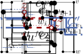
(b) Vertical.

(c) Horizontal.

(d) Horizontal.

(e) Horizontal.

Figure 29: Examples of augmentations. (29(a)) The candidate edges of $u$ are $e_{1}$, $e_{2}$ and $e_{3}$. (29(b)) Insertion of vertical edge $uz$. (29(c)) $\Gamma^{u}_{vw}$ contains a decreasing cycle. (29(d)) $\Gamma^{u}_{vw}$ is valid. (29(e)) Insertion of horizontal edge $uw_{i}$ because there is a horizontal path from $w_{i}$ to $u$.

The rectangulation procedure works by augmenting non-rectangular faces one by one, thereby successively removing concave angles at the vertices until all faces are rectangles. Traversing the boundary of a face in clockwise direction yields a sequence of left and right turns, where a degree-1 vertex contributes two left turns. Note that concave angles correspond exactly to left turns in this sequence. Consider a face $f$ with a left turn (i.e., a concave angle) at $u$ such that the following two turns when walking along $f$ (in clockwise direction) are right turns; see Figure 29. We call $u$ a port of $f$. We define a set of candidate edges that contains precisely those edges $vw$ of $f$, for which $\operatorname{rot}(f[u,vw])=2$; see Figure 29(a). We treat this set as a sequence, where the edges appear in the same order as in $f$, beginning with the first candidate after $u$. The augmentation $\Gamma^{u}_{vw}$ with respect to a candidate edge $vw$ is obtained by splitting the edge $vw$ into the edges $vz$ and $zw$, where $z$ is a new vertex, and adding the edge $uz$ in the interior of $f$ such that the angle formed by $zu$ and the edge following $u$ on $f$ is $90\degree$. The direction of the new edge $uz$ in $\Gamma^{u}_{vw}$ is the same for all candidate edges. If this direction is vertical, we call $u$ a vertical port and otherwise a horizontal port. We note that any vertex with a concave angle in a face becomes a port during the augmentation process. For regular faces Tamassia [31] shows that they always contain a port. Moreover, the following observation can be proven analogously.

Observation 3.

If $u$ is a port of a face $f$ and $vw$ is a candidate edge for $u$, then $\Gamma^{u}_{vw}$ is an ortho-radial representation.

However, an augmentation $\Gamma^{u}_{vw}$ is not necessarily valid. We prove that we can always find an augmentation that is valid. The crucial ingredient is the following proposition.

Proposition 2.

Let $G$ be a planar 4-graph with valid ortho-radial representation $\Gamma$, let $f$ be a regular face of $G$ and let $u$ be a port of $f$ with candidate edges $e_{1}=v_{1}w_{1},\dots,e_{k}=v_{k}w_{k}$. Then the following facts hold:

1. If $u$ is a vertical port, then $\Gamma^{u}_{e_{1}}$ is a valid ortho-radial representation; see Figure 29(b)

2. If $u$ is a horizontal port, then $\Gamma^{u}_{e_{1}}$ does not contain an increasing cycle and $\Gamma^{u}_{e_{k}}$ does not contain a decreasing cycle; see Figure 29(c)–29(d).

3. Let $P_{i}$ be the maximal path that contains the vertex $w_{i}$ of the candidate edge $e_{i}=v_{i}w_{i}$ and that consists of only horizontal edges. If $u$ is a horizontal port and $\Gamma^{u}_{e_{i}}$ contains a decreasing cycle and $\Gamma^{u}_{e_{i+1}}$ contains an increasing cycle, then $u$ is an endpoint of $P_{i}$ and adding the horizontal edge $uz$ to the other endpoint $z$ of $P_{i}$ yields a horizontal cycle; see Figure 29(e). In particular, $\Gamma+uz$ is valid.

To increase the readability we split the proof of Proposition 2 into the separate Lemmas 14– 17, which we defer to Section 7.2.

We are now ready describe the rectangulation procedure. Let $G$ be a planar 4-graph with valid ortho-radial representation $\Gamma$. Without loss of generality, we can assume that $G$ is connected, otherwise we can treat the connected components separately. We further insert triangles in both the central and outer face and suitably connect these to the original graph; see Figure 30. Namely, for the central face $g$ we identify an edge $e$ on the simple cycle $C$ bounding $g$ such that $\ell_{C}(e)=0$. Since $\Gamma$ is valid and $C$ is an essential cycle, such an edge exists. We then insert a new cycle $C^{\prime}$ of length 3 inside $g$ and connect one of its vertices to a new vertex on $e$. The new cycle $C^{\prime}$ now forms the boundary of the central face. Analogously, we insert into the outer face a cycle $C_{o}$ of length $3$ which contains $G$ and is connected to the reference edge $e^{\star}$. We choose an arbitrary edge $e^{\star\star}$ on $C_{o}$ as new reference edge. We observe that there is a path $P$ from $e^{\star\star}$ to $e^{\star}$ with rotation $0$. Hence, each reference path from $e^{\star}$ to an essential cycle in $\Gamma$ can be extended by $P$ such that the new path is a reference path with respect to $e^{\star\star}$ and has the same rotation.

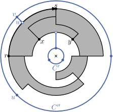
Figure 30: The outer and the central face are rectangulated by adding cycles of length 3. The cycle $C^{\prime}$ is connected to an arbitrary edge $xy$ that has label 0 and $C^{\prime\prime}$ is connected to a new vertex on the old reference edge $rs$. The edge $uv$ is selected as the new reference edge.

After this preprocessing any face $f$ that is not a rectangle is regular, and it therefore contains a port $u$. If any of the candidate augmentations $\Gamma^{u}_{e_{i}}$ is valid, then $\Gamma^{u}_{e_{i}}$ has fewer concave corners than $\Gamma$, and we continue the augmentation procedure with $\Gamma^{u}_{e_{i}}$. On the other hand, if none of these augmentations is valid, then each $\Gamma^{u}_{e_{i}}$ contains a strictly monotone cycle. Let $i$ be the smallest index such that $\Gamma^{u}_{e_{i}}$ contains an increasing cycle and note that such an index $i$ exists and that $i>1$ by property 2 of Proposition 2. Then, by definition of $i$, $\Gamma^{u}_{e_{i-1}}$ contains a decreasing cycle and $\Gamma^{u}_{e_{i}}$ contains an increasing cycle. But then property 3 of Proposition 2 guarantees the existence of a vertex $z$ such that $\Gamma+uz$ is valid and has fewer concave corners than $\Gamma$. Using this procedure we can iteratively augment $\Gamma$ to a rectangular ortho-radial representation that contains a subdivision of the ortho-radial representation $\Gamma$.

7.2 Proof of Proposition 2

Throughout this section, we assume that we are in the situation described by Proposition 2. That is, $G$ is a planar 4-graph with valid ortho-radial representation $\Gamma$, and $u$ is a port of a regular face $f$ with candidate edges $e_{1}=v_{1}w_{1},\dots,e_{k}=v_{k}w_{k}$. After possibly replacing $\Gamma$ with $\mathrm{flip}(\Gamma)$, we may assume that the edge $uz$ resulting from an augmentation with a candidate is directed to the right or up. By Lemma 6 there is a one-to-one correspondence between increasing (decreasing) cycles in $\Gamma$ and increasing (decreasing) cycles in $\mathrm{flip}(\Gamma)$.

Lemma 14.

If $u$ is a vertical port, then $\Gamma^{u}_{e_{1}}$ is a valid ortho-radial representation.

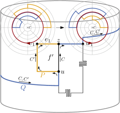
Figure 31: Illustration of proof for Lemma 14. In this illustration it is assumed that inserting the edge $uz$ into a valid ortho-radial representation creates an increasing cycle $C$ that uses $uz$. However, then there is cycle $C^{\prime}$ not using $uz$ that is also increasing.

Proof.

Assume for the sake of contradiction that $\Gamma^{u}_{e_{1}}$ contains a strictly monotone cycle $C$. As $\Gamma$ is valid, $C$ must contain the new edge $uz$ in either direction (i.e., $uz$ or $zu$). Let $f^{\prime}$ be the new rectangular face of $G+uz$ containing $u$, $v_{1}$ and $z$, and consider the subgraph $H=C+f^{\prime}$ of $G+uz$. According to Lemma 11 there exists an essential cycle $C^{\prime}$ that does not contain $uz$. Moreover, $C^{\prime}$ can be decomposed into paths $P$ and $Q$ such that $P$ lies on $f^{\prime}$ and $Q$ is a part of $C$; see Figure 31.

The goal is to show that $C^{\prime}$ is increasing or decreasing. We present a proof only for the case that $C$ is an increasing cycle. The proof for decreasing cycles can be obtained by flipping all inequalities.

For each edge $e$ on $Q$ the labels $\ell_{C}(e)$ and $\ell_{C^{\prime}}(e)$ are equal by Lemma 11, and hence $\ell_{C^{\prime}}(e)\leq 0$. For an edge $e\in P$, there are two possible cases: $e$ either lies on the side of $f^{\prime}$ parallel to $uz$ or on one of the two other sides. In the first case, the label of $e$ is equal to the label $\ell_{C}(uz)$ ($\ell_{C}(zu)$ if $C$ contains $zu$ instead of $uz$). In particular the label is negative.

In the second case, we first note that $\ell_{C^{\prime}}(e)$ is even, since $e$ points left or right. Assume that $\ell_{C^{\prime}}(e)$ was positive and therefore at least $2$. Then, let $e^{\prime}$ be the first edge on $C^{\prime}$ after $e$ that points to a different direction. Such an edge exists, since otherwise $C^{\prime}$ would be an essential cycle whose edges all point to the right, but they are not labeled with 0. This edge $e^{\prime}$ lies on $Q$ or is parallel to $uz$. Hence, the argument above implies that $\ell_{C^{\prime}}(e^{\prime})\leq 0$. However, $\ell_{C^{\prime}}(e^{\prime})$ differs from $\ell_{C^{\prime}}(e)$ by at most $1$, which requires $\ell_{C^{\prime}}(e^{\prime})\geq 1$. Therefore, $\ell_{C^{\prime}}(e)$ cannot be positive.

We conclude that all edges of $C^{\prime}$ have a non-positive label. If all labels were $0$, $C$ would not be an increasing cycle by Proposition 1. Thus, there exists an edge on $C^{\prime}$ with a negative label and $C^{\prime}$ is an increasing cycle in $\Gamma$. But as $\Gamma$ is valid, such a cycle does not exist, and therefore $C$ does not exist either. Hence, $\Gamma^{u}_{e_{1}}$ is valid. ∎∎

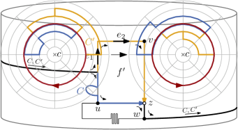
Figure 32: The increasing cycle $C$ contains $uz$. There are three possibilities for edges on $C^{\prime}$ that lie not on $C$: They lie on the left side of $f^{\prime}$ (like $e_{1}$), on the top (like $e_{2}$), or on the right side formed by only the edge $vz$.

Lemma 15.

If $u$ is a horizontal port, then $\Gamma^{u}_{e_{1}}$ contains no increasing cycle.

Proof.

Let $f^{\prime}$ be the new rectangular face of $\Gamma^{u}_{e_{1}}$ containing $u$, $v_{1}$ and $z$, and assume for the sake of contradiction that there is an increasing cycle $C$ in $\Gamma^{u}_{e_{1}}$. This cycle must use either $uz$ or $zu$. Similar to the proof of Lemma 14, we find an increasing cycle $C^{\prime}$ in $\Gamma$, contradicting the validity of $\Gamma$.

Applying Lemma 11 to $C$ and $f^{\prime}$ yields an essential cycle $C^{\prime}$ without $uz$ and $zu$ that can be decomposed into a path $P$ on $f^{\prime}$ and a path $Q\subseteq C\setminus f^{\prime}$ such that all edges of $Q$ have non-positive labels. We show in the following that the edges of $P$ also have non-positive labels.

If $C$ contains $uz$, there are three possibilities for an edge $e$ of $P$, which are illustrated in Figure 32: The edge $e$ lies on the left side of $f^{\prime}$ and points up, $e$ is parallel to $uz$, or $e=v_{1}z$. In the first case $\ell_{C^{\prime}}(e)=\ell_{C}(uz)-1<0$ and in the second case $\ell_{C^{\prime}}(e)=\ell_{C}(uz)\leq 0$. If $e=v_{1}z$, $C$ cannot contain $zv_{1}$ and therefore $zw_{1}\in C$. Then, $\ell_{C^{\prime}}(e)=\ell_{C}(zw_{1})<0$. In all three cases the label of $e$ is at most 0.

If $C$ contains $zu$, the label of $zu$ has to leave a remainder of 2 when it is divided by 4 since $zu$ points to the left. As the label is also at most $0$, we conclude $\ell_{C}(zu)\leq-2$. The edges of $P$ lie either on the left, top or right of $f^{\prime}$. Therefore, the label of any edge $e$ on $P$ differs by at most 1 from $\ell_{C}(zu)$, and thus we get $\ell_{C^{\prime}}(e)\leq 0$.

Summarizing the results above, we see that all edges on $C^{\prime}$ are labeled with non-positive numbers. The case that all labels of $C^{\prime}$ are equal to 0 can be excluded, since $C$ would not be an increasing cycle by Proposition 1. Hence, $C^{\prime}$ is an increasing cycle, which was already present in $\Gamma$, contradicting the validity of $\Gamma$. ∎∎

Lemma 16.

If $u$ is a horizontal port, then $\Gamma^{u}_{e_{k}}$ contains no decreasing cycle.

Proof.

Let $uz$ be the new edge inserted in $\Gamma^{u}_{e_{k}}$. In $\Gamma^{u}_{e_{k}}$, the face $f$ is split in two parts. Let $f^{\prime}$ be the face containing $v_{k}$ and $f^{\prime\prime}$ the one containing $w_{k}$. Assume for the sake of contradiction that there is a decreasing cycle $C$ in $\Gamma^{u}_{e_{k}}$. Then, either $uz$ or $zu$ lies on $C$. By Lemma 11 there exists an essential cycle $C^{\prime}$ that can be decomposed into a path $P$ on $f^{\prime\prime}$ and $Q=C\cap C^{\prime}$; see Figure 33(a). For all edges $e\in E(Q)$, we have $\ell_{C}(e)=\ell_{C^{\prime}}(e)\geq 0$ by Lemma 11. Since $C^{\prime}$ is already present in $\Gamma$ and $\Gamma$ is valid, $C^{\prime}$ cannot be decreasing. Moreover, since $C$ and $C^{\prime}$ intersect, $C^{\prime}$ cannot be horizontal by Proposition 1. Therefore, $C^{\prime}$ must contain an edge $xy$ with $\ell_{C^{\prime}}(xy)<0$, which hence has to lie on $P$.

(a)

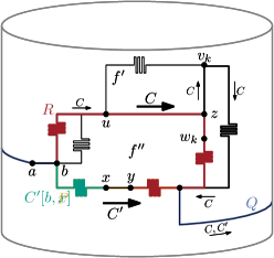
(b)

Figure 33: The situation in the proof of Lemma 16. The cycle $C$ is decreasing and it is assumed that $\ell_{C^{\prime}}(xy)<0$. (a) The decomposition of $C^{\prime}$ into $P$ and $Q$. (b) The reference paths $R$ and $C^{\prime}[b,x]$ from $ab$ to $xy$.

Our goal is to show that there must be a candidate on $f$ after $y$ and in particular after the last candidate $e_{k}$—a contradiction. The following claim gives a sufficient condition for the existence of such a candidate.

Claim 1: If $\operatorname{rot}(f[u,yx])\leq 2$, then there is a candidate on $f[yx,u]$. To prove Claim 33, we determine for each edge $e$ on $f$ the value $r(e):=\operatorname{rot}(f[u,e])$. By assumption, it is $r(yx)\leq 2$. For the last edge $e_{\text{last}}$ on $f[yx,u]$ it is $r(e_{\text{last}})=\operatorname{rot}(f)-\operatorname{rot}(tuv)=5$, where $t$ and $v$ are the preceding and succeeding vertices of $u$ on $f$, respectively. Here, we use that $f$ is a regular face (i.e., $\operatorname{rot}(f)=4$) and $\operatorname{rot}(tuv)=-1$ since $u$ is a port.

Note that for two consecutive edges $e,e^{\prime}$ on the boundary of $f$, it is $r(e^{\prime})\leq r(e)+1$. Therefore, there exists an edge $e$ that lies between $yx$ and $e_{\text{last}}$ on the boundary of $f$ that satisfies $r(e)=2$. Hence, $e$ is a candidate that lies after $yx$ on the boundary of $f$. ${\diamond}$

To finish the proof of the lemma it hence suffices to show that $\operatorname{rot}(f[u,yx])\leq 2$. As $e_{k}$ is a candidate, we have $\operatorname{rot}(f[u,zw_{k}])=2$ and therefore

$$\operatorname{rot}(f[u,yx])=\operatorname{rot}(f[u,zw_{k}])+\operatorname{rot}(f[zw_{k},yx])=\operatorname{rot}(f[zw_{k},yx])+2.$$

Thus, it suffices to show $\operatorname{rot}(f[zw_{k},yx])\leq 0$.

We present a detailed argument for the case that $C$ uses $uz$ as illustrated in Figure 33. At the end of the proof, we briefly outline how the argument can be adapted if $C$ uses $zu$.

If $C$ uses $uz$, then $P$ is directed such that $f^{\prime\prime}$ lies to the left of $P$. Thus, $C^{\prime}$ lies in the interior of $C$. Let now $ab$ be the last edge of $Q$, and let $R$ be the path defined by $C[b,uz]+f[zw_{k},y]$; see Figure 33(b). Both $R$ and $C^{\prime}[b,x]$ are reference paths from $ab$ to $xy$ that lie in the interior of $C$ and in the exterior of $C^{\prime}$. Applying the second statement of Lemma 3 hence gives

$$\operatorname{dir}(ab,R,xy)=\operatorname{dir}(ab,C^{\prime}[b,x],xy).$$ (7)

The direction along $R$ is defined as

$$\operatorname{dir}(ab,R,xy) =\operatorname{rot}(ab+R+yx)-2$$

$$=\operatorname{rot}(ab+C[b,uz]+f[zw_{k},y]+yx)-2$$

$$=\operatorname{rot}(C[ab,uz]+f[zw_{k},yx])-2$$

$$=\operatorname{rot}(C[ab,uz])+\operatorname{rot}(uzw_{k})+\operatorname{rot}(f[zw_{k},yx])-2$$

$$=\ell_{C}(uz)-\ell_{C}(ab)+\operatorname{rot}(f[zw_{k},yx])-1.$$

The last step uses $\operatorname{rot}(C[ab,uz])=\ell_{C}(uz)-\ell_{C}(ab)$ and $\operatorname{rot}(uzw_{k})=1$.

The rotation along $C^{\prime}[b,x]$ is defined as

$$\operatorname{dir}(ab,C^{\prime}[b,x],xy) =\operatorname{rot}(ab+C^{\prime}[b,x]+xy)$$

$$=\operatorname{rot}(C^{\prime}[ab,xy])$$

$$=\ell_{C^{\prime}}(xy)-\ell_{C^{\prime}}(ab)$$

$$=\ell_{C^{\prime}}(xy)-\ell_{C}(ab).$$

The last step uses that $\ell_{C}(ab)=\ell_{C^{\prime}}(ab)$ by Lemma 11. Altogether, we obtain

$$\ell_{C}(uz)-\ell_{C}(ab)+\operatorname{rot}(f[zw_{k},yx])-1=\ell_{C^{\prime}}(xy)-\ell_{C}(ab),$$

which can be rearranged to

$$\operatorname{rot}(f[zw_{k},yx])=\ell_{C^{\prime}}(xy)-\ell_{C}(uz)+1.$$

With $\ell_{C^{\prime}}(xy)\leq-1$ and $\ell_{C}(uz)\geq 0$ we obtain $\operatorname{rot}(f[zw_{k},yx])\leq 0$. This completes the proof for the case that $uz$ lies on $C$.

If $zu$ lies on $C$, we consider the flipped representation $\mathrm{flip}(\Gamma^{u}_{e_{k}})$. In $\mathrm{flip}(\Gamma^{u}_{e_{k}})$ the cycle $\mkern 1.5mu\overline{\mkern-1.5muC\mkern-1.5mu}\mkern 1.5mu$ is decreasing and contains the edge $uz$. The cycle $\mkern 1.5mu\overline{\mkern-1.5muC^{\prime}\mkern-1.5mu}\mkern 1.5mu$ is not decreasing and contains the edge $yx$ with label $\mkern 1.5mu\overline{\mkern-1.5mu\ell\mkern-1.5mu}\mkern 1.5mu_{\mkern 1.5mu\overline{\mkern-1.5muC^{\prime}\mkern-1.5mu}\mkern 1.5mu}(yx)=\ell_{C^{\prime}}(xy)<0$. Moreover, the cycle $\mkern 1.5mu\overline{\mkern-1.5muC\mkern-1.5mu}\mkern 1.5mu$ contains $\mkern 1.5mu\overline{\mkern-1.5muC^{\prime}\mkern-1.5mu}\mkern 1.5mu$ in its interior. Thus, the argument above can be applied to $\mkern 1.5mu\overline{\mkern-1.5muC\mkern-1.5mu}\mkern 1.5mu$, $\mkern 1.5mu\overline{\mkern-1.5muC^{\prime}\mkern-1.5mu}\mkern 1.5mu$, and $yx$ instead of $C$, $C^{\prime}$, and $xy$. ∎∎

Lemma 17.

Let $P_{i}$ be the maximal path that contains the vertex $w_{i}$ of the candidate edge $e_{i}=v_{i}w_{i}$ and that consists of only horizontal edges. If $u$ is a horizontal port and $\Gamma^{u}_{e_{i}}$ contains a decreasing cycle and $\Gamma^{u}_{e_{i+1}}$ contains an increasing cycle, then $u$ is an endpoint of $P_{i}$ and adding the horizontal edge $uz$ to the other endpoint $z$ of $P_{i}$ yields a horizontal cycle. In particular, $\Gamma+uz$ is valid.

(a)

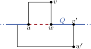
(b)

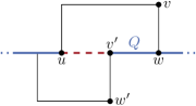
(c)

Figure 34: Three possibilities how the path between $w$ and $v^{\prime}$ can look like: 34(a) $w=v^{\prime}$, 34(b) all edges point right, and 34(c) all edges point left. In the first two cases the edge $uw$ is inserted and in (c) $uv^{\prime}$ is added.

Proof.

(a)

(b)

(c)

Figure 35: Illustration of proof for Lemma 17. (35(a)) $\Gamma^{u}_{e_{i}}$ is obtained by inserting the edge $uz_{i}$ into $\Gamma$. (35(b)) $\Gamma^{u}_{e_{i+1}}$ is obtained by inserting the edge $uz_{i+1}$ into $\Gamma$. (35(c)) $\tilde{\Gamma}$ is obtained by combining $\Gamma^{u}_{e_{i}}$ and $\Gamma^{u}_{e_{i+1}}$.

Let $z_{i}$ be the new vertex inserted in $\Gamma^{u}_{e_{i}}$ and $z_{i+1}$ the one in $\Gamma^{u}_{e_{i+1}}$. Since both $uz_{i}$ and $uz_{i+1}$ point to the right, there is no augmentation of $\Gamma$ containing both edges. We compare $\Gamma^{u}_{e_{i}}$ and $\Gamma^{u}_{e_{i+1}}$ by the following construction (see also Figure 35), which models all important aspects of both representations: Starting from $\Gamma$ we insert new vertices $z_{i}$ on $e_{i}$ and $z_{i+1}$ on $e_{i+1}$. We connect $u$ and $z_{i}$ by a path of length 2 that points to the right and denote its internal vertex by $x$. Furthermore, a path of length 2 from $x$ via a new vertex $y$ to $z_{i+1}$ is added. The edge $xy$ points down and $yz_{i+1}$ to the right. In the resulting ortho-radial representation $\tilde{\Gamma}$ the edge $uz_{i}$ in $\Gamma^{u}_{e_{i}}$ is modeled by the path $uxz_{i}$. Similarly, the edge $uz_{i+1}$ in $\Gamma^{u}_{e_{i+1}}$ is modeled by the path $uxyz_{i+1}$ in $\tilde{\Gamma}$.

Take any decreasing cycle in $\Gamma^{u}_{e_{i}}$. As $\Gamma$ is valid, this cycle must contain either $uz_{i}$ or $z_{i}u$. We obtain a cycle $C_{1}$ in $\tilde{\Gamma}$ by replacing $uz_{i}$ with $uxz_{i}$ (or $z_{i}u$ with $z_{i}xu$). Note that $ux$ and $xz_{i}$ have the same label as $uz_{i}$, and the labels of all other edges on the cycles stay the same by Lemma 12. Therefore, $C_{1}$ is a decreasing cycle.

Similarly, there exists an increasing cycle $C^{\prime}_{1}$ in $\Gamma^{u}_{e_{i+1}}$, which contains $uz_{i+1}$ or $z_{i+1}u$. Replacing $uz_{i+1}$ with $uxyz_{i+1}$ (or $z_{i+1}u$ with $z_{i+1}yxu$) we get a cycle $C_{2}$ in $\tilde{\Gamma}$. By Lemma 12 the labels of $C_{2}$ are non-positive outside of $uxyz_{i+1}$ (or $z_{i+1}yxu$) and there is an edge with negative label. Consequently, the only edge of $C_{2}$ that may have a positive label is the edge $e$ between $x$ and $y$. Since $C_{1}$ and $C_{2}$ intersect, Lemma 10 implies that $C_{2}$ is not increasing. Thus, the label of $e$ is positive. If $e=yx$, then $\ell_{C_{2}}(e)\geq 3$ and its succeeding edge has a positive label as well. Hence, the cycle $C_{2}$ contains the edge $xy$ and consequently the edge $ux$.

Using this construction we show that one endpoint of $P_{i}$ is $u$ and the other is another vertex of $f$. To that end, we prove the following claims.

Claim 1: The cycles $C_{1}$ and $C_{2}$ both contain the edge $ux$ and it is $\ell_{C_{1}}(ux)=\ell_{C_{2}}(ux)=0$.

Claim 2: The vertices $w_{i}$ and $v_{i+1}$ have a degree of at least 2. Further, $C_{1}$ contains $w_{i}$ and $C_{2}$ contains $v_{i+1}$.

Claim 3: The edges of $f[w_{i},v_{i+1}]$ are part of $P_{i}$. In particular, $C_{2}$ contains $w_{i}$ or $C_{1}$ contains $v_{i+1}$.

Claim 4: The right endpoint of $P_{i}$ is $u$ and the left endpoint $z$ lies on $f$.

Using these claims we prove the lemma as follows. Due to Claim 7.2 we can insert the horizontal edge $uz$ into $\Gamma$ obtaining a horizontal cycle $P_{i}+uz$. The resulting ortho-radial representation is valid, because any strictly monotone cycle necessarily contains $uz$ and hence shares a vertex with a horizontal cycle, contradicting Lemma 1. This finishes the proof. In the following we prove the claims.

Figure 36: Illustration of proof for Claim 7.2 of Lemma 17.

Claim 7.2. Let $H=C_{1}+C_{2}$ be the graph formed by the two cycles $C_{1}$ and $C_{2}$ and let $\tilde{f}$ be its central face. Assume that the edge $ux$ is not incident to $\tilde{f}$. As both $C_{1}$ and $C_{2}$ contain $ux$ (or $xu$), the face $\tilde{f}$ consists of edges of both $C_{1}$ and $C_{2}$. In particular, there is an edge $e$ of $C_{2}\setminus C_{1}$ on $\tilde{f}$ whose source $v$ lies on $C_{1}$; see Figure 36. Let $x_{1}$ and $x_{2}$ be the succeeding vertices of $v$ on $C_{1}$ and $C_{2}$, respectively. As $C_{1}$ is a decreasing cycle, we have $\ell_{C_{1}}(vx_{1})\geq 0$. If $\ell_{C_{2}}(vx_{2})\leq 0$, then by Lemma 9 the edge $e=vx_{2}$ lies in the exterior of $C_{1}$, which contradicts the choice of $e$. Hence, we have $\ell_{C_{2}}(vx_{2})>0$, which implies that $e=xy$. Further, the cyclic order of the vertex $x$ implies that $ux$ is the predecessor of $xy$ on the central face, which contradicts the assumption that $ux$ is not incident to $\tilde{f}$.

Since $C_{2}$ contains $ux$, the central face $\tilde{f}$ lies to the right of $ux$. Since $C_{1}$ is also directed such that $\tilde{f}$ lies to the right of $C_{1}$, it cannot contain $xu$, but it contains $ux$. By Lemma 8 we further obtain that $\ell_{C_{1}}(ux)=\ell_{C_{2}}(ux)=0$.

Claim 7.2. We consider the setting in $\tilde{\Gamma}$; see Figure 35(c). From Claim 7.2 we obtain $\ell_{C_{1}}(xz_{i})=0$. Consequently, since $C_{1}$ is a decreasing cycle and since $\operatorname{rot}(xz_{i}w_{i})=1$ and $\operatorname{rot}(xz_{i}v_{i})=-1$, the cycle contains the edge $z_{i}w_{i}$ but not the edge $z_{i}v_{i}$. In particular, this implies that $w_{i}$ has a degree of at least 2, as otherwise $C_{1}$ would not be simple. Similarly, from Claim 7.2 we obtain $\ell_{C_{1}}(yz_{i+1})=0$. Consequently, since $C_{2}$ has only non-positive labels except on $xy$ and since $\operatorname{rot}(xz_{i+1}v_{i+1})=-1$ and $\operatorname{rot}(xz_{i+1}w_{i+1})=1$, the cycle contains the edge $z_{i+1}v_{i+1}$ but not the edge $z_{i+1}w_{i+1}$. In particular, this implies that $v_{i+1}$ has a degree of at least 2, as otherwise $C_{2}$ would not be simple.

Claim 7.2. Let $e_{s}$ be the direct successor of $e_{i}$ and let $e_{p}$ be the direct predecessor of $e_{i+1}$ on the boundary of $f$. In order to show the claim, we do a case distinction on the rotations $\operatorname{rot}(e_{i},e_{s})$ and $\operatorname{rot}(e_{p},e_{i+1})$. From Claim 7.2 it follows that $\operatorname{rot}(e_{i},e_{s})\in\{-1,0,1\}$ and $\operatorname{rot}(e_{p},e_{i+1})\in\{-1,0,1\}$. Further, it cannot be both $\operatorname{rot}(e_{i},e_{f})=1$ and $\operatorname{rot}(e_{p},e_{i+1})=1$. Otherwise, since $\operatorname{rot}(f[u,e_{i}])=2$ and $\operatorname{rot}(f[u,e_{i+1}])=2$, it would hold $\operatorname{rot}(f[u,e_{s}])=3$ and $\operatorname{rot}(f[u,e_{p}])=1$. In that case, there would be a further candidate edge $e$ with $\operatorname{rot}(f[u,e])=2$ between $e_{i}$ and $e_{i+1}$. Thus, we obtain $\operatorname{rot}(e_{i},e_{s})\in\{-1,0\}$ or $\operatorname{rot}(e_{p},e_{i+1})\in\{-1,0\}$,

First, assume that $\operatorname{rot}(e_{i},e_{s})=0$. We obtain $e_{s}=e_{i+1}$ and hence $e_{p}=e_{i}$. Otherwise, $e_{s}$ would be a candidate edge between $e_{i}$ and $e_{i+1}$. Consequently, $f[w_{i},v_{i+1}]$, which consist of the single vertex $v=w_{i}=v_{i+1}$, trivially belongs to $P_{i}$. Moreover, by Claim 7.2 the cycle $C_{2}$ then also contains $w_{i}$ and $C_{1}$ contains $v_{i+1}$. The very same argument can be applied for $rot(e_{p},e_{i+1})=0$, as we also obtain $e_{s}=e_{i+1}$ and $e_{p}=e_{i}$. In particular, we obtain $\operatorname{rot}(e_{i},e_{s})=0$ if and only if $\operatorname{rot}(e_{p},e_{i+1})=0$.

(a)

(b)

Figure 37: Illustration of proof for Claim 7.2 of Lemma 17.

Now, assume that $\operatorname{rot}(e_{i},e_{s})=-1$ or $\operatorname{rot}(e_{p},e_{i+1})=-1$. We first consider the case that $\operatorname{rot}(e_{i},e_{s})=-1$; see Figure 37(a). We observe that $C_{1}$ contains $e_{s}$ as it also contains the vertex $w_{i}$ by Claim 7.2. Let $Q_{i}$ be the maximal horizontal path on $f$ that starts at $w_{i}$. We observe that $Q_{i}$ is a prefix of $P_{i}$, and the cycle $C_{1}$ shares at least $e_{s}$ with $Q_{i}$. Since by Claim 7.2 the cycle $C_{1}$ has label $0$ on $ux$, it also has label $0$ on any of its edges that lie on $Q_{i}$. In fact, this implies that $C_{1}$ completely contains the path $Q_{i}$. Otherwise, it would contain an edge that does not belong $Q_{i}$, but starts at an intermediate vertex of $Q_{i}$. By the choice of $Q_{i}$ such an edge has a negative label since its preceding edge has label $0$, which contradicts that $C_{1}$ is decreasing. For the same reason, the edge $e$ that succeeds $Q_{i}$ on $f$ has a negative label. Hence, the edge $e$ is the candidate $e_{i+1}$. Consequently, $C_{1}$ contains $v_{i+1}$ and $f[w_{i},v_{i+1}]=Q_{i}$, which shows Claim 7.2. For the case that $\operatorname{rot}(e_{l},e_{i+1})=-1$ we use similar arguments; see Figure 37(b). Let $Q_{i+1}$ be the maximal horizontal path on $f$ that starts at $v_{i+1}$ when going along $f$ counterclockwise. The first edge of $Q_{i+1}$ is $e_{p}$, which also belongs to $C_{2}$. Further, $C_{2}$ has label $0$ on any of its edges that belong to $Q_{i+1}$. Consequently, $C_{2}$ contains $Q_{i+1}$ completely, as otherwise it would contain an edge that points downwards, contradicting that $C_{2}$ has only non-positive labels except for the edge $xy$. Hence, the edge of $f$ that is incident with the endpoint of $Q_{i+1}$ and does not belong to $Q_{i+1}$ is the candidate edge $e_{i}$, which concludes the proof.

Claim 7.2. We first show that $u$ is the right endpoint of $P_{i}$. To that end, let $H=C_{1}+C_{2}$ be the graph formed by the two cycles $C_{1}$ and $C_{2}$ and let $\tilde{f}$ be its central face. From the proof of Claim 7.2 we know that $ux$ is incident to the central face. Further, from Claim 7.2 and Claim 7.2 it follows that $C_{1}$ and $C_{2}$ have the vertex $w_{i}$ or the vertex $v_{i+1}$ in common; see Figure 37(a) and Figure 37(b), respectively. Let $v=w_{i}$ in the former case and let $v=v_{i+1}$ in the latter case.

We first show that $C_{1}[v,x]=C_{2}[v,x]$. Assume that this is not the case. Consider the maximal common prefix of $C_{1}[v,x]$ and $C_{2}[v,x]$, and let $w$ be the endpoint of that prefix. As $v$ is incident to $\tilde{f}$, this also applies to $w$. Further, by Lemma 9 the outgoing edge of $w$ on $C_{2}$ lies in the exterior of $C_{1}$. Let $t$ be the first intersection of $C_{1}$ and $C_{2}$ on $\tilde{f}$ after $w$. Then the edge to $t$ on $C_{2}$ lies strictly in the exterior of $C_{1}$ contradicting Lemma 9.

Hence, we have $C_{1}[v,x]=C_{2}[v,x]$; we denote that path by $P$. Since $ux$ is incident to $\tilde{f}$, all edges of $P$ are incident to $\tilde{f}$ as well. Hence, by Corollary 2 all edges of $P$ have label 0 on $C_{1}$ and $C_{2}$ and are therefore horizontal. As $f[w_{i},v_{i+1}]$ also belongs to $P_{i}$, we conclude that $u$ is the right endpoint of $P_{i}$.

(a)

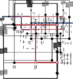
(b)

Figure 38: Illustration of proof for Claim 7.2 of Lemma 17.

Finally, we argue that $z$ belongs to the face $f$. As by Claim 7.2 $f[w_{i},v_{i+1}]$ belongs to $P_{i}$, the vertex $z$ belongs to a prefix $P$ of $P_{i}$ that does not contain any edge of $f[w_{i},v_{i+1}]$ and ends either at $w_{i}$ or at $v_{i+1}$; see Figure 38(a) and Figure 38(b), respectively. If $P$ is empty, $w_{i}$ or $v_{i+1}$ is $z$, respectively, which shows the claim. So assume that $P$ is not empty. Let $vw$ be the last edge of $P$, i.e., depending on the considered case we either have $w=w_{i}$ or $w=v_{i+1}$. By the local ordering of the incident edges of $w$, the path $P$ lies in the interior of $f$. Further, $vw$ is incident to $f$ on both sides, as otherwise the two other incident edges of $w$ could not be incident to $f$ as well. Hence, we obtain $\operatorname{rot}(f[u,wv])=3$ and $\operatorname{rot}(f[u,vw])=0$. Thus, the path $f[wv,vw]$ of $f$ consists only of horizontal edges, as otherwise there would be an edge $e$ on that path with $\operatorname{rot}(f[u,e])=2$, which contradicts the choice of $e_{i}$ and $e_{i+1}$. Altogether, the path $f[wv,vw]$ is $\mkern 1.5mu\overline{\mkern-1.5muP\mkern-1.5mu}\mkern 1.5mu+P$, which proves that $z$ belongs to $f$. ∎∎

7.3 Proof of the Main Theorem

We are now ready to prove the characterization of drawable ortho-radial representations.

Proof.

(a)

(b)

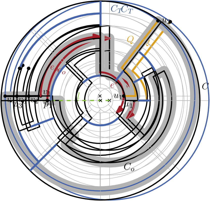
(c)

Figure 39: Illustration of proof for Theorem 3.2.

If $\Gamma$ is a valid ortho-radial representation, then using the rectangulation procedure of Section 7.1 we obtain a valid rectangular ortho-radial representation $\Gamma^{\prime}$ that contains a subdivision of $\Gamma$. Then $\Gamma^{\prime}$ has a drawing $\Delta^{\prime}$ by Theorem 3, and a drawing $\Delta$ of $\Gamma$ is obtained from $\Delta^{\prime}$ by removing edges that are in $\Gamma^{\prime}$ but not in $\Gamma$, and by undoing subdivisions. It remains to show that the reference edge $e^{\star}$ of $\Gamma$ is an outlying edge in $\Delta$, which then implies that $\Gamma$ is drawable.

Let $C_{o}$ be the essential cycle that is part of the outer face of $\Gamma$ and let $e_{o}$ be an outermost horizontal edge of $C_{o}$ in $\Delta$, i.e., an horizontal edge of $C_{o}$ with maximum distance to the center; see Figure 39(a). If $e_{o}$ can be chosen as the reference edge $e^{\star}$, then $e^{\star}$ is an outlying edge of $\Delta$. Hence, assume that $e_{o}$ cannot be chosen as $e^{\star}$.

Let $C_{T}$ be the essential cycle that forms the outer face of $\Gamma^{\prime}$. Further, let $l$ be the ray that emanates from the center of $\Delta^{\prime}$ and goes through the source vertex $v$ of $e_{o}$. Let $p_{1},\dots,p_{k}$ be the intersection points of $l$ with $\Delta^{\prime}$ from $v$ on. We observe that $p_{1}=v$ and $p_{k}$ lies on $C_{T}$. For each intersection point $p_{i}$ with $1\leq i\leq k$ we insert a vertex $v_{i}$ at $p_{i}$ if there is no vertex so far. Further, we add vertical edges to $\Delta^{\prime}$ such that the new drawing contains the path $P=v_{1}\dots v_{k}$. We denote the resulting drawing by $\Delta^{\prime\prime}$; see Figure 39(b).

By the construction of the rectangulation the drawing $\Delta^{\prime\prime}$ further contains a path $Q$ that connects a subdivision vertex $u_{1}$ on $e^{\star}$ with a vertex $u_{2}$ on $C_{T}$. We observe that the cycle $C=C_{o}[v_{1},u_{1}]+Q+T[u_{2},v_{k}]+\mkern 1.5mu\overline{\mkern-1.5muP\mkern-1.5mu}\mkern 1.5mu$ is essential. Moreover, by construction the path $C[u_{1},v_{1}]=Q+C_{T}[u_{2},v_{k}]+\mkern 1.5mu\overline{\mkern-1.5muP\mkern-1.5mu}\mkern 1.5mu$ has rotation 2. Since $C$ has a left bend at both $v_{1}$ and $u_{1}$ it follows that $C_{o}[v_{1},u_{1}]$ has rotation 0. Consequently, $e^{\star}$ is an outlying edge in $\Delta$. Altogether, we obtain that $\Gamma$ is drawable.

Conversely, assume that $\Gamma$ is drawable. Hence, $\Gamma$ has a drawing $\Delta$ in which the reference edge $e^{\star}$ of $\Gamma$ is an outlying edge. By Lemma 5 we can assume without loss of generality that $e^{\star}$ lies on the outermost circle that is used by an essential cycle of $\Delta$. By [23] the representation $\Gamma$ satisfies Conditions 1 and 2 of Definition 1. To prove that $\Gamma$ is valid, we show how to reduce the general case to the more restricted one, where all faces are rectangles. By Corollary 3 the existence of a drawing and the validity of the ortho-radial representation are equivalent.

Given the drawing $\Delta$, we augment it such that all faces are rectangles. This rectangulation is similar to the one described in Section 7.1 but works with a drawing and not only with a representation. We first insert the missing parts of the innermost and outermost circle that are used by $\Delta$ such that the outer and the central face are already rectangles. For each left turn on a face $f$ at a vertex $u$, we then cast a ray from $v$ in $f$ in the direction in which the incoming edge of $u$ points. This ray intersects another edge in $\Delta$. Say the first intersection occurs at the point $p$. Either there already is a vertex $z$ drawn at $p$ or $p$ lies on an edge. In the latter case, we insert a new vertex, which we call $z$, at $p$. We then insert the edge $uz$ in $G$ and update $\Delta$ and $\Gamma$ accordingly.

Repeating this step for all left turns, we obtain a drawing $\Delta^{\prime}$ and an ortho-radial representation $\Gamma^{\prime}$ of the augmented graph $G^{\prime}$; see Figure 39(c) for an example of $\Delta^{\prime}$. As the labelings of essential cycles are unchanged by the addition of edges elsewhere in the graph, any increasing or decreasing cycle in $\Gamma$ would also appear in $\Gamma^{\prime}$. But by Corollary 3 $\Gamma^{\prime}$ is valid, and hence neither $\Gamma$ nor $\Gamma^{\prime}$ contain increasing or decreasing cycles. Thus, $\Gamma$ is valid. ∎∎

We remark that the proof of Theorem 3.2 is in fact constructive and it can easily be implemented in polynomial time, provided that we can check in polynomial time whether a given ortho-radial representation is valid. We develop such an algorithm with running time $\mathcal{O}(n^{2})$ in Section 8. In Section 9 we show how compute a rectangulation of $\Gamma$ in time $\mathcal{O}(n^{2})$.

8 Validity Testing

In this section, we show how to check whether a given ortho-radial representation is valid in polynomial time, which yields the following statement.

The two conditions for ortho-radial representations are local and checking them can easily be done in linear time. Throughout this section, we therefore assume that we are given an instance $I=(G,\mathcal{E},f_{c},f_{o})$ with an ortho-radial representation $\Gamma$ and a reference edge $e^{\star}$. The condition for validity however references all essential cycles of which there may be exponentially many. We present an algorithm that checks whether $\Gamma$ contains a strictly monotone cycle and computes such a cycle if one exists. The main difficulty is that the labels on a decreasing cycle $C$ depend on a reference path $P$ that runs from $e^{\star}$ to $C$ and respects $C$. However, we know neither the path $P$ nor the cycle $C$ in advance, and choosing a specific cycle $C$ may rule out certain paths $P$ and vice versa.

We only describe how to search for decreasing cycles; increasing cycles can be found by searching for decreasing cycles in the mirrored representation by Lemma 7. A decreasing cycle $C$ is outermost if it is not contained in the interior of any other decreasing cycle. Clearly, if $\Gamma$ contains a decreasing cycle, then it also has an outermost one. We first show that in this case this cycle is uniquely determined.

Lemma 18.

If $\Gamma$ contains a decreasing cycle, there is a unique outermost decreasing cycle.

Proof.

Assume that $\Gamma$ has two outermost decreasing cycles $C_{1}$ and $C_{2}$, i.e., $C_{1}$ does not lie in the interior of $C_{2}$ and vice versa. Let $C$ be the cycle bounding the outer face of the subgraph $H=C_{1}+C_{2}$ that is formed by the two decreasing cycles. By construction, $C_{1}$ and $C_{2}$ lie in the interior of $C$, and we claim that $C$ is a decreasing cycle contradicting that $C_{1}$ and $C_{2}$ are outermost. To that end, we show that $\ell_{C}(e)=\ell_{C_{1}}(e)$ for any edge $e$ that belongs to both $C$ and $C_{1}$, and $\ell_{C}(e)=\ell_{C_{2}}(e)$ for any edge $e$ that belongs to both $C$ and $C_{2}$. Hence, all edges of $C$ have a non-negative label since $C_{1}$ and $C_{2}$ are decreasing. By Proposition 1 there is at least one label of $C$ that is positive, and hence $C$ is a decreasing cycle.

It remains to show that $\ell_{C}(e)=\ell_{C_{1}}(e)$ for any edge $e$ that belongs to both $C$ and $C_{1}$; the case that $e$ belongs to both $C$ and $C_{2}$ can be handled analogously. Let $\Gamma_{H}$ be the ortho-radial representation $\Gamma$ restricted to $H$. We flip the cylinder to exchange the outer face with the central face and vice versa. More precisely, Lemma 6 implies that the reverse edge $\mkern 1.5mu\overline{\mkern-1.5mue\mkern-1.5mu}\mkern 1.5mu$ of $e$ lies on the central face of the flipped representation $\mathrm{flip}(\Gamma_{H})$ of $\Gamma_{H}$. Further, it proves that $\mkern 1.5mu\overline{\mkern-1.5mu\ell\mkern-1.5mu}\mkern 1.5mu_{\mkern 1.5mu\overline{\mkern-1.5muC\mkern-1.5mu}\mkern 1.5mu}(\mkern 1.5mu\overline{\mkern-1.5mue\mkern-1.5mu}\mkern 1.5mu)=\ell_{C}(e)$ and $\mkern 1.5mu\overline{\mkern-1.5mu\ell\mkern-1.5mu}\mkern 1.5mu_{\mkern 1.5mu\overline{\mkern-1.5muC_{1}\mkern-1.5mu}\mkern 1.5mu}(\mkern 1.5mu\overline{\mkern-1.5mue\mkern-1.5mu}\mkern 1.5mu)=\ell_{C_{1}}(e)$, where $\mkern 1.5mu\overline{\mkern-1.5mu\ell\mkern-1.5mu}\mkern 1.5mu$ is the labeling in $\mkern 1.5mu\overline{\mkern-1.5mu\Gamma_{H}\mkern-1.5mu}\mkern 1.5mu$. Hence, by Corollary 2 we obtain $\mkern 1.5mu\overline{\mkern-1.5mu\ell\mkern-1.5mu}\mkern 1.5mu_{\mkern 1.5mu\overline{\mkern-1.5muC\mkern-1.5mu}\mkern 1.5mu}(\mkern 1.5mu\overline{\mkern-1.5mue\mkern-1.5mu}\mkern 1.5mu)=\mkern 1.5mu\overline{\mkern-1.5mu\ell\mkern-1.5mu}\mkern 1.5mu_{\mkern 1.5mu\overline{\mkern-1.5muC_{1}\mkern-1.5mu}\mkern 1.5mu}(\mkern 1.5mu\overline{\mkern-1.5mue\mkern-1.5mu}\mkern 1.5mu)$. Flipping back the cylinder, again by Lemma 6 we obtain $\ell_{C}(e)=\ell_{C_{1}}(e)$. ∎∎

The core of our algorithm is an adapted left-first DFS. Given a directed edge $e$ it determines the outermost decreasing cycle $C$ in $\Gamma$ such that $C$ contains $e$ in the given direction and $e$ has the smallest label among all edges on $C$, if such a cycle exists. By running this test for each directed edge of $G$ as the start edge, we find a decreasing cycle if one exists.

More precisely, the DFS visits each vertex at most once and it maintains for each visited vertex $v$ a reference edge $\mathrm{ref}(v)$, the edge of the search tree via which $v$ was visited. Whenever it has a choice which vertex to visit next, it picks the first outgoing edge in clockwise direction after the reference edge that leads to an unvisited vertex. In addition to that, we employ a filter that ignores certain outgoing edges during the search. To that end, we define for all outgoing edges $e$ incident to a visited vertex $v$ a search label $\tilde{\ell}(e)$ by setting $\tilde{\ell}(e)=\tilde{\ell}(\mathrm{ref}(v))+\operatorname{rot}(\mathrm{ref}(v)+e)$ for each outgoing edge $e$ of $v$. In our search we ignore edges with negative search labels. For a given directed edge $vw$ in $G$ we initialize the search by setting $\mathrm{ref}(w)=vw$, $\tilde{\ell}(vw)=0$ and then start searching from $w$.

Let $T$ denote the directed search tree with root $w$ constructed by the DFS in this fashion. If $T$ contains $v$, then this determines a candidate cycle $C$ containing the edge $vw$. If $C$ is a decreasing cycle, which we can easily check by determining a reference path, we report it. Otherwise, we show that there is no outermost decreasing cycle $C$ such that $vw$ lies on $C$ and has the smallest label among all edges on $C$.

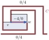
Figure 40: The search from $vw$ finds the non-decreasing cycle $C$. Edges are labeled $\ell_{C}(e)/\tilde{\ell}(e)$.

It is necessary to check that $C$ is essential and decreasing. For example the cycle in Figure 40 is found by the search and though it is essential, it is non-decreasing. This is caused by the fact that the label of $vw$ is actually $-4$ on this cycle but the search assumes it to be $0$.

Figure 41: Path $Q$ and its prefix $P$ that leaves $C$ once and ends at a vertex $p$ of $C$.

Lemma 19.

Assume that $\Gamma$ contains a decreasing cycle. Let $C$ be the outermost decreasing cycle of $\Gamma$ and let $vw$ be an edge on $C$ with the minimum label, i.e., $\ell_{C}(vw)\leq\ell_{C}(e)$ for all edges $e$ of $C$. Then the left-first DFS from $vw$ finds $C$.

Proof.

Assume for the sake of contradiction that the search does not find $C$. Let $T$ be the tree formed by the edges visited by the search. Since the search does not find $C$ by assumption, a part of $C[w,v]$ does not belong to $T$. Let $xy$ be the first edge on $C[w,v]$ that is not visited, i.e., $C[w,x]$ is a part of $T$ but $xy\not\in T$. There are two possible reasons for this. Either $\tilde{\ell}(xy)<0$ or $y$ has already been visited before via another path $Q$ from $w$ with $Q\neq C[w,y]$.

The case $\tilde{\ell}(xy)<0$ can be excluded as follows. By the construction of the labels $\tilde{\ell}$, for any path $P$ from $w$ to a vertex $z$ in $T$ and any edge $e^{\prime}$ incident to $z$ we have $\tilde{\ell}(e^{\prime})=\operatorname{rot}(vw+P+e^{\prime})$. In particular, $\tilde{\ell}(xy)=\operatorname{rot}(C[vw,xy])=\ell_{C}(xy)-\ell_{C}(vw)\geq 0$ since the rotation can be rewritten as a label difference (see Observation 2) and $vw$ has the smallest label on $C$.

Hence, $T$ contains a path $Q$ from $w$ to $x$ that was found by the search before and $Q$ does not completely lie on $C$. There is a prefix of $Q$ (possibly of length $0$) lying on $C$ followed by a subpath not on $C$ until the first vertex $p$ of $Q$ that again belongs to $C$; see Figure 41. We set $P=Q[w,p]$ and denote the vertex where $P$ leaves $C$ by $b$. By construction the edge $vw$ lies on $C[p,b]$. The subgraph $H=P+C$ that is formed by the decreasing cycle $C$ and the path $P$ consists of the three internally vertex-disjoint paths $P[b,p]$, $C[b,p]$ and $\mkern 1.5mu\overline{\mkern-1.5muC\mkern-1.5mu}\mkern 1.5mu[b,p]$ between $b$ and $p$. Since edges that are further left are preferred during the search, the clockwise order of these paths around $b$ and $p$ is fixed as in Figure 41. In $H$ there are three faces, bounded by $C$, $\mkern 1.5mu\overline{\mkern-1.5muC\mkern-1.5mu}\mkern 1.5mu[b,p]+\mkern 1.5mu\overline{\mkern-1.5muP\mkern-1.5mu}\mkern 1.5mu[p,b]$ and $P[b,p]+\mkern 1.5mu\overline{\mkern-1.5muC\mkern-1.5mu}\mkern 1.5mu[p,b]$, respectively. Since $C$ is an essential cycle and it bounds a face in $H$, it bounds the central face and one of the two other faces is the outer face. These two possibilities are shown in Figure 42. We denote the cycle bounding the outer face but in which the edges are directed such that the outer face lies locally to the left by $C^{\prime}$. That is, the boundary of the outer face is $\mkern 1.5mu\overline{\mkern-1.5muC^{\prime}\mkern-1.5mu}\mkern 1.5mu$. We distinguish cases based on which of the two possible cycles constitutes $\mkern 1.5mu\overline{\mkern-1.5muC^{\prime}\mkern-1.5mu}\mkern 1.5mu$.

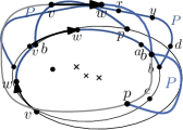
(a) The edge $vw$ lies on the outer face of $H$.

(b) The edge $vw$ does not lie on the outer face of $H$.

Figure 42: The two possible embeddings of the subgraph formed by the decreasing cycle $C$ and the path $P$, which was found by the search.

If $\mkern 1.5mu\overline{\mkern-1.5muC^{\prime}\mkern-1.5mu}\mkern 1.5mu=\mkern 1.5mu\overline{\mkern-1.5muC\mkern-1.5mu}\mkern 1.5mu[b,p]+\mkern 1.5mu\overline{\mkern-1.5muP\mkern-1.5mu}\mkern 1.5mu[p,b]$ forms the outer face of $H$, $vw$ lies on $C^{\prime}$ as illustrated in Figure 42(a) and we show that $C^{\prime}$ is a decreasing cycle, which contradicts the assumption that $C$ is the outermost decreasing cycle. Since $P$ is simple and lies in the exterior of $C$, the path $P$ is contained in $C^{\prime}$, which means $C^{\prime}[w,p]=P$. The other part of $C^{\prime}$ is formed by $C[p,w]$. Since $C$ forms the central face of $H$, the labels of the edges on $C[p,w]$ are the same for $C$ and $C^{\prime}$ by Proposition 8. In particular, $\ell_{C}(vw)=\ell_{C^{\prime}}(vw)$ and all the labels of edges on $C[p,w]$ are non-negative because $C$ is decreasing. The label of any edge $e$ on both $C^{\prime}$ and $P$ is $\ell_{C^{\prime}}(e)=\ell_{C^{\prime}}(vw)+\operatorname{rot}(vw+P[w,e])=\ell_{C}(vw)+\tilde{\ell}(e)\geq 0$. Thus, the labeling of $C^{\prime}$ is non-negative. Further, not all labels of $C^{\prime}$ are $0$ since otherwise $C$ would not be a decreasing cycle by Proposition 1. Hence, $C^{\prime}$ is decreasing and contains $C$ in its interior, a contradiction.

If $\mkern 1.5mu\overline{\mkern-1.5muC^{\prime}\mkern-1.5mu}\mkern 1.5mu=\mkern 1.5mu\overline{\mkern-1.5muC\mkern-1.5mu}\mkern 1.5mu[p,b]+P[b,p]$, the edge $vw$ does not lie on $C^{\prime}$; see Figure 42(b). We show that $C^{\prime}$ is a decreasing cycle containing $C$ in its interior, again contradicting the choice of $C$. As above, Proposition 8 implies that the common edges of $C$ and $C^{\prime}$ have the same labels on both cycles. It remains to show that all edges $xy$ on $\mkern 1.5mu\overline{\mkern-1.5muP\mkern-1.5mu}\mkern 1.5mu[p,b]$ have non-negative labels. To establish this we use paths to the edge that follows $b$ on $C$. This edge $bc$ has the same label on both cycles and thus provides a handle on $\ell_{C^{\prime}}(xy)$. We make use of the following equations, which follow immediately from the definition of the (search) labels.

$$\ell_{C^{\prime}}(bc) =\ell_{C^{\prime}}(xy)+\operatorname{rot}(\mkern 1.5mu\overline{\mkern-1.5muP\mkern-1.5mu}\mkern 1.5mu[xy,db])+\operatorname{rot}(dbc)=\ell_{C^{\prime}}(xy)-\operatorname{rot}(P[bd,yx])-\operatorname{rot}(cbd)$$

$$\ell_{C}(bc) =\ell_{C}(vw)+\operatorname{rot}(C[vw,ab])+\operatorname{rot}(abc)$$

$$\tilde{\ell}(yx) =\operatorname{rot}(C[vw,ab])+\operatorname{rot}(abd)+\operatorname{rot}(P[bd,yx])$$

Since $\ell_{C}(bc)=\ell_{C^{\prime}}(bc)$ and $\operatorname{rot}(abd)=-\operatorname{rot}(dba)$, we thus get

$$\ell_{C^{\prime}}(xy) =\ell_{C}(vw)+\operatorname{rot}(C[vw,ab])+\operatorname{rot}(abc)+\operatorname{rot}(P[bd,yx])+\operatorname{rot}(cbd)$$

$$=\ell_{C}(vw)+\tilde{\ell}(yx)+\operatorname{rot}(dba)+\operatorname{rot}(abc)+\operatorname{rot}(cbd).$$

Since $\ell_{C}(vw)\geq 0$ and $\tilde{\ell}(yx)\geq 0$ (as $yx$ was not filtered out), it follows that $\ell_{C^{\prime}}(xy)\geq\operatorname{rot}(abc)+\operatorname{rot}(dba)+\operatorname{rot}(cbd)=2$ as this is the sum of clockwise rotations around a degree-3 vertex. Hence, $C^{\prime}$ is decreasing and contains $C$ in its interior, a contradiction. Since both embeddings of $H$ lead to a contradiction, we obtain a contradiction to our initial assumption that the search fails to find $C$. ∎∎

The left-first DFS clearly runs in $\mathcal{O}(n)$ time. In order to guarantee that the search finds a decreasing cycle if one exists, we run it for each of the $\mathcal{O}(n)$ directed edges of $G$. Since some edge must have the lowest label on the outermost decreasing cycle, Lemma 19 guarantees that we eventually find a decreasing cycle if one exists. Increasing cycles can be found by searching for decreasing cycles in the mirror representation $\mathrm{mirror}(\Gamma)$ (Lemma 7). Altogether, this proves Theorem 3.2.

9 Efficient Rectangulation Procedure

Let $G$ be a planar 4-graph with valid ortho-radial representation $\Gamma$. By Theorem 3.2 $\Gamma$ is drawable. The proof of Theorem 3.2 is constructive and shows how to augment $\Gamma$ to a valid rectangular ortho-radial representation $\Gamma^{\star}$. Then a drawing $\Delta^{\star}$ of $\Gamma^{\star}$ can be computed by determining flows in two flow networks by Theorem 13. A drawing $\Delta$ of $\Gamma$ can be finally obtained by undoing augmentation steps. Hence, it remains to show how a valid ortho-radial representation can be rectangulated efficiently.

To follow the construction of the proof of Theorem 3.2, one needs to determine efficiently whether an augmentation yields a valid ortho-radial representation $\Gamma^{u}_{vw}$. We call such an augmentation a valid augmentation. Since each valid augmentation reduces the number of concave angles, we obtain a rectangulation after $\mathcal{O}(n)$ valid augmentations. Moreover, there are $\mathcal{O}(n)$ candidates for each augmentation, each of which can be tested for validity (and increasing/decreasing cycles can be detected) in $\mathcal{O}(n^{2})$ time by Theorem 3.2. Thus, the rectangulation algorithm can be implemented to run in $\mathcal{O}(n^{4})$ time.

In the remainder of this section we present an improvement to $\mathcal{O}(n^{2})$ time, which is achieved in three steps. First, we show that, due to the nature of augmentations, each validity test can be done in $\mathcal{O}(n)$ time. This reduces the running time of the augmentation procedure to $\mathcal{O}(n^{3})$; see Section 9.1. Second, we show how to find a valid augmentation for a given port $u$ using only $\mathcal{O}(\log n)$ validity tests, thus improving the running time to $\mathcal{O}(n^{2}\log n)$; see Section 9.2. Finally, we design an algorithm that can be used to post-process a valid augmentation and which reduces the number of validity tests to $\mathcal{O}(n)$ and the running time to $\mathcal{O}(n^{2})$ in total; see Section 9.3. Altogether, this proves our third main result.

9.1 1st Improvement – Faster Validity Test

The general test for strictly monotone cycles performs one left-first DFS per edge and runs in $\mathcal{O}(n^{2})$ time. However, we can exploit the special structure of the augmentation to reduce the running time to $\mathcal{O}(n)$. For the proof we restrict ourselves to the case that the inserted edge $uz$ points to the right. The case that it points left can be handled by flipping the representation using Lemma 6.

The key result is that in any decreasing cycle of an augmentation the new edge $uz$ has the minimum label. Thus, performing only one left-first DFS starting at $uz$ is sufficient. For increasing cycles the arguments do not hold, but in a second step we show that the test for increasing cycles can be replaced by a simple test for horizontal paths.

Recall that the augmentations $\Gamma^{u}_{vw}$ that are tested during the rectangulation are built by adding one edge $uz$ to a valid representation $\Gamma$. Hence, any strictly monotone cycle in $\Gamma^{u}_{vw}$ contains the edge $uz$.

We first show that the new edge $uz$ has label $0$ on any decreasing cycle in the augmentation $\Gamma^{u}_{vw}$ if $vw$ is the first candidate. We extend this result afterwards to augmentations to all candidates. Since the label of edges on decreasing cycles is non-negative, this implies in particular that the label of $uz$ is minimum, which is sufficient for the left-first DFS to succeed (see Lemma 19).

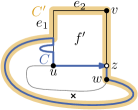
Figure 43: A decreasing cycle $C$ that uses $uz$ and an essential cycle $C^{\prime}$ derived from $C$.

Lemma 20.

Let $\Gamma$ be a valid ortho-radial representation and let $u$ be a horizontal port on $f$ with first candidate $vw$. If $\Gamma^{u}_{vw}$ contains a decreasing cycle $C$, then $C$ contains $uz$ in this direction and $\ell_{C}(uz)=0$.

Proof.

We first consider the case that $C$ uses $uz$ (and not $zu$) and assume for the sake of contradiction that $\ell_{C}(uz)\neq 0$; see Figure 43. Since $uz$ points right, $\ell_{C}(uz)$ is divisible by $4$. Together with $\ell_{C}(uz)\geq 0$ because $C$ is decreasing, we obtain $\ell_{C}(uz)\geq 4$. By Lemma 11 there is an essential cycle $C^{\prime}$ without $uz$ in the subgraph $H$ that is formed by the new rectangular face $f^{\prime}$ and $C$. We show that $C^{\prime}$ is a decreasing cycle. We observe that each edge of $C^{\prime}$ either lies on $f^{\prime}$ or is an edge of $C$. For any $e\in C^{\prime}\cap C$ Lemma 11 gives $\ell_{C^{\prime}}(e)=\ell_{C}(e)\geq 0$. Since $f^{\prime}$ is rectangular, the labels of edges in $C^{\prime}\cap f^{\prime}$ differ by at most $1$ from $\ell_{C}(uz)$. By assumption it is $\ell_{C}(uz)\geq 4$ and therefore $\ell_{C^{\prime}}(e)\geq 3$ for all edges $e\in C^{\prime}\cap f^{\prime}$. Hence, $C^{\prime}$ is a decreasing cycle in $G$ contradicting the validity of $\Gamma$.

If $zu\in C$, it is $\ell_{C}(zu)\geq 2$ and a similar argument yields a decreasing cycle in $\Gamma$. ∎∎

While the same statement does not generally hold for all candidates, it does hold if the first candidate creates a decreasing cycle.

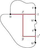
Figure 44: The structure used to simulate the simultaneous insertion of $uz$ to $vw$ and $uz^{\prime}$ to $v^{\prime}w^{\prime}$.

Lemma 21.

Let $\Gamma$ be a valid ortho-radial representation and let $u$ be a horizontal port on $f$ with first candidate $vw$. Further, let $v^{\prime}w^{\prime}$ be another candidate and denote the edge inserted in $\Gamma^{u}_{v^{\prime}w^{\prime}}$ by $uz^{\prime}$. If $\Gamma^{u}_{vw}$ contains a decreasing cycle, any decreasing cycle $C^{\prime}$ in $\Gamma^{u}_{v^{\prime}w^{\prime}}$ uses $uz^{\prime}$ in this direction and $\ell_{C^{\prime}}(uz^{\prime})=0$.

Proof.

In order to simulate the simultaneous insertion of two new edges to both $vw$ and $v^{\prime}w^{\prime}$ we use the structure from the proof of Lemma 17; see Figure 44. We denote the resulting augmented representation by $\tilde{\Gamma}$. There is a one-to-one correspondence between decreasing cycles in $\Gamma^{u}_{vw}$ and decreasing cycles in $\tilde{\Gamma}$ containing $uxz$. Let $C$ be a decreasing cycle in $\tilde{\Gamma}$ containing $uxz$. By Lemma 20 the cycle $C$ contains $uxz$ in this direction, and we have $\ell_{C}(ux)=0$.

Similarly, for any decreasing cycle in $\Gamma^{u}_{v^{\prime}w^{\prime}}$ there is a cycle in $\tilde{\Gamma}$ where $uz^{\prime}$ ($z^{\prime}u$) is replaced by the path $uxyz^{\prime}$ ($z^{\prime}yxu$). Let $\tilde{C^{\prime}}$ be the cycle in $\tilde{\Gamma}$ that corresponds to the decreasing cycle $C^{\prime}$ in $\Gamma^{u}_{v^{\prime}w^{\prime}}$.

Suppose for now that $C^{\prime}$ uses $uz^{\prime}$ in this direction, which means that $\tilde{C^{\prime}}$ uses $ux$. In particular, since $\ell_{\tilde{C^{\prime}}}(ux)=\ell_{C^{\prime}}(uz^{\prime})$, it holds $\ell_{\tilde{C^{\prime}}}(xy)=\ell_{\tilde{C^{\prime}}}(ux)+1\geq 1$. Let $\tilde{f}$ be the central face of $H=\tilde{C}+\tilde{C^{\prime}}$. We note that $\tilde{f}$ is a decreasing cycle by Lemma 8 and Proposition 1. Since $\Gamma$ is valid, $\tilde{f}$ is not exclusively formed by edges of $G$. Thus, by the construction of $H$, the path $uxyz^{\prime}$ lies on $\tilde{f}$. Lemma 8 therefore implies that $\ell_{\tilde{C^{\prime}}}(ux)=\ell_{C}(ux)=0$, where the last equality follows from Lemma 20.

Above we assumed that $C^{\prime}$ uses $uz^{\prime}$ in this direction. This is in fact the only possibility. Assume for the sake of contradiction that $C^{\prime}$ contains $z^{\prime}u$ and hence $xu\in\tilde{C^{\prime}}$. As above we can argue that the central face $\tilde{f}$ of $\tilde{C}+\tilde{C}^{\prime}$ is not exclusively formed by edges of $G$ and that the path $z^{\prime}yxz$ lies on $\tilde{f}$. By Lemma 8 we have $\ell_{\tilde{C^{\prime}}}(yx)=\ell_{C}(xz)-\operatorname{rot}(yxz)=-1$. Hence, we obtain $\ell_{C^{\prime}}(z^{\prime}u)=\ell_{\tilde{C^{\prime}}}(xu)=\ell_{\tilde{C^{\prime}}}(yx)+\operatorname{rot}(yxu)=-2$, which contradicts that $C^{\prime}$ is a decreasing cycle. ∎∎

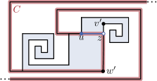
Figure 45: Here, the insertion of the edge $uz$ to the last candidate $v^{\prime}w^{\prime}$ introduces an increasing cycle $C$ with $\ell_{C}(uz)=-4$.

Altogether, we can efficiently test which of the candidates $e_{1},\dots,e_{k}$ produce decreasing cycles as follows. By Lemma 20, if the first candidate is not valid, then $\Gamma^{u}_{e_{1}}$ has a decreasing cycle that contains the new edge $uz$ with label $0$, which is hence the minimum label for all edges on the cycle. This can be tested in $\mathcal{O}(n)$ time by Lemma 19. Fact 2 of Proposition 2 guarantees that we either find a valid augmentation or a decreasing cycle. In the former case we are done, in the second case Lemma 21 allows us to similarly restrict the labels of $uz$ to $0$ for the remaining candidate edges, thus allowing us to detect decreasing cycles in $\Gamma^{u}_{e_{i}}$ in $\mathcal{O}(n)$ time for $i=2,\dots,k$.

It is tempting to use the mirror symmetry (Lemma 7) to exchange increasing and decreasing cycles to deal with increasing cycles in an analogous fashion. However, this fails as mirroring invalidates the property that $u$ is followed by two right turns in clockwise direction. For example, in Figure 45 inserting the edge to the last candidate introduces an increasing cycle $C$ with $\ell_{C}(uz)=-4$. We therefore give a direct algorithm for detecting increasing cycles in this case.

Let $e_{i}=v_{i}w_{i}$ and $e_{i+1}={v_{i+1}w_{i+1}}$ be two consecutive candidates for $u$ such that $\Gamma^{u}_{e_{i}}$ contains a decreasing cycle but $\Gamma^{u}_{e_{i+1}}$ does not. If $\Gamma^{u}_{e_{i+1}}$ contains an increasing cycle, then by Fact 3 of Proposition 2 the vertices $w_{i}$, $v_{i+1}$ and $u$ lie on a horizontal path that starts at a vertex $z$ incident to $f$ and ends at $u$. The presence of such a horizontal path $P$ can clearly be checked in linear time, thus allowing us to also detect increasing cycles provided that the previous candidate produced a decreasing cycle. If $P$ exists, we insert the edge $uz$. By Proposition 1 this does not produce strictly monotone cycles. Otherwise, if $P$ does not exist, the augmentation $\Gamma^{u}_{e_{i+1}}$ is valid. In both cases we have resolved the horizontal port $u$ successfully.

Summarizing, the overall algorithm for augmenting from a horizontal port $u$ now works as follows. By exploiting Lemmas 20 and 21, we test the candidates in the order as they appear on $f$ until we find the first candidate $e$ for which $\Gamma^{u}_{e}$ does not contain a decreasing cycle. Using Fact 3 of Proposition 2 we either find that $\Gamma^{u}_{e}$ is valid, or we find a horizontal path as described above. In both cases this allows us to determine an edge whose insertion does not introduce a strictly monotone cycle. Since in each test for a decreasing cycle the edge $uz$ can be restricted to have label $0$, each of the tests takes linear time. This improves the running time of the rectangulation algorithm to $\mathcal{O}(n^{3})$.

9.2 2nd Improvement – Fewer Validity Tests

Instead of linearly searching for a suitable candidate for $u$, we can employ a binary search on the candidates, which reduces the number of validity tests for $u$ from linear to logarithmic. To do this efficiently, we first compute the list of all candidates $e_{1},\dots,e_{k}$ for $u$ in time linear in the size of $f$. Next, we test if the augmentation $\Gamma^{u}_{e_{1}}$ is valid. If it is, we are done.

Otherwise, we start the binary search on the list $e_{1},\dots,e_{k}$, where $k$ is the number of candidates for $u$. The search maintains a sublist $e_{i},\dots,e_{j}$ of consecutive candidates such that $\Gamma^{u}_{e_{i}}$ contains a decreasing cycle and $\Gamma^{u}_{e_{j}}$ does not. Note that this invariant holds in the beginning, because we explicitly test for a decreasing cycle in $\Gamma^{u}_{e_{1}}$ and there is no decreasing cycle in $\Gamma^{u}_{e_{k}}$ by Fact 2 of Proposition 2. If the list consists of only two consecutive candidates, i.e., $j=i+1$, we stop. Otherwise, we set $m=\lfloor(i+j)/2\rfloor$ and test if $\Gamma^{u}_{e_{m}}$ contains a decreasing cycle. If it does, we recurse on $e_{m},\dots,e_{j}$ and otherwise on $e_{i},\dots,e_{m}$. As the invariant is preserved, we end up with two consecutive candidates $e_{i}$ and $e_{i+1}$ such that $\Gamma^{u}_{e_{i}}$ contains a decreasing cycle and $\Gamma^{u}_{e_{i+1}}$ does not. In this situation Fact 3 of Proposition 2 guarantees that we find a valid augmentation. Clearly this only requires $O(\log n)$ validity tests in total. Further, as argued in the previous subsection each of these tests can be performed in linear time. Altogether, we obtain the following lemma.

Lemma 22.

Using binary search we find a valid augmentation for $u$ in $\mathcal{O}(n\log n)$ time.

Since there are $\mathcal{O}(n)$ ports to remove, we obtain that any planar $4$-graph with valid ortho-radial representation can be rectangulated in $\mathcal{O}(n^{2}\log n)$ time.

Theorem 2.

Given a valid ortho-radial representation $\Gamma$, a corresponding rectangulation can be computed in $\mathcal{O}(n^{2}\log n)$ time.

9.3 3rd Improvement – Linear Number of Validity Tests

In this section we describe an improvement of our algorithm that reduces the total number of validity tests to $\mathcal{O}(n)$ such that the running time of our algorithm becomes $\mathcal{O}(n^{2})$. The improvement adapts the augmentation step for horizontal ports of the rectangulation procedure. Let $u$ be a horizontal port of a face $f$ and let $e_{1},\dots,e_{k}$ be its candidate edges. The adapted augmentation step resolves $u$ in two steps.

(a) $\Gamma_{1}$: $r_{2}r_{3}$ points right.

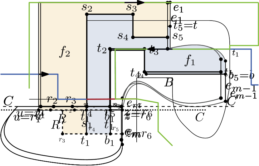
(b) $\Gamma_{1}$: $r_{2}r_{3}$ points downwards.

Figure 46: Illustration of Step 1, which inserts $R$, $T$ and $B$ into $\Gamma_{0}$. Depending on whether $uz$ lies on a horizontal cycle $C$ in $\Gamma_{0}$, the edge $r_{2}r_{3}$ points (46(a)) to the right or (46(b)) downwards.

• We do a linear scan on $e_{1},\dots,e_{k}$ to search for the first candidate $e_{m}$ of $u$ that gives rise to a valid augmentation with an additional edge $uz$. Recall that $z$ either subdivides $e_{m}$ or $uz$ completes a horizontal cycle that contains the source of $e_{m}$. We note that we apply $m$ validity tests in this step. In case that $m<4$, the augmentation step is stopped. Otherwise we continue with the following step.

• In the following let $\Gamma_{0}$ be the valid ortho-radial representation that we obtain after Step 1. We observe that the inserted edge $uz$ splits the face $f$ into two smaller faces. In Step 2.1 we partition the face that contains the edges $e_{1},\dots,e_{m-1}$ by inserting two paths $T$ and $B$ of constant size that start at subdivision vertices on $uz$ and end at subdivision vertices on $e_{1}$ and $e_{m-1}$, respectively; see Figure 46. These two paths separate two sub-faces $f_{1}$ and $f_{2}$ of $f$ that contain the candidate edges $e_{1},\dots,e_{m-2}$, which are all but a constant number of edges for which we have performed validity tests in Step 1. In Step 2.2. we rectangulate $f_{1}$ without performing any validity test and in Step 2.3 we rectangulate $f_{2}$ performing a number of validity tests that is proportional to the size of $f_{2}$. In the following we describe the three steps in greater detail.

  • We adapt $\Gamma_{0}$ as follows. We introduce a path $B=b_{1}\dots b_{5}$ in $f$ that connects a subdivision vertex $b_{1}$ on $uz$ with a subdivision vertex on $e_{m-1}$; see Figure 46. The edge $b_{1}b_{2}$ points upwards, the edge $b_{3}b_{4}$ points downwards, and the other two edges point to the right. The face that lies to the left of $B$ is the face $f^{\prime}$ we seek to rectangulate. Similarly, we introduce a path $T=t_{1}\dots t_{5}$ in $f^{\prime}$ that connects a subdivision vertex $t_{1}$ on $ub_{1}$ with a subdivision vertex on $e_{1}$. The edge $t_{1}t_{2}$ points upwards, the edge $t_{3}t_{4}$ points downwards, and the other two edges point to the right. Finally, we subdivide the edge $ut_{1}$ by two additional vertices. Altogether, the edge $uz$ has been replaced by a path $R=r_{1}\dots r_{6}$ with $r_{1}=u$, $r_{4}=t_{1}$, $r_{5}=b_{1}$ and $r_{6}=z$. As we have obtained the edges of $R$ by subdividing $uz$, they all point to the right. In the case that $uz$ does not lie on a horizontal cycle, we orient $r_{2}r_{3}$ such that it points downwards.

    We denote the resulting ortho-radial representation by $\Gamma_{1}$. Further, let $f_{1}$ be the face that lies to the right of $T$, and let $f_{2}$ be the face that lies to the left of $T$.

  • We iteratively resolve the ports in $f_{1}$ until the face is rectangulated. For each port $u^{\prime}$ of $f_{1}$ we augment the ortho-radial representation as follows. If $u^{\prime}$ is a vertical port, we augment with respect to the first candidate edge and if $u^{\prime}$ is a horizontal port we augment with respect to the last candidate edge of $u^{\prime}$. The procedure stops when $f_{1}$ is completely rectangulated. We denote the resulting ortho-radial representation by $\Gamma_{2}$. We emphasize that this step does not execute any validity test.

  • Starting with $\Gamma_{2}$, we rectangulate the face $f_{2}$, which has a constant number of ports, by iteratively applying the original augmentation step. We denote the resulting ortho-radial representation by $\Gamma_{3}$.

In the following we show that the modified rectangulation procedure runs in $\mathcal{O}(n^{2})$ time and yields a valid ortho-radial representation.

Lemma 23.

The modified rectangulation procedure produces a valid, rectangulated ortho-radial representation.

Since the proof is rather technical, we defer it to Section 23. In the following we argue the running time. To that end, we first prove that the output rectangulation has linear size.

Lemma 24.

The rectangulated ortho-radial representation produced by the modified rectangulation procedure has size $\mathcal{O}(n)$.

Proof.

For the proof we define the potential function

$$\Phi=3\cdot\text{horizontal corners of }\Gamma+\text{vertical corners of }\Gamma,$$

where a horizontal (vertical) corner is a concave corner that becomes a horizontal (vertical) port of a face during the rectangulation procedure. At the beginning of the rectangulation procedure it holds $\Phi\leq 4n$, because each vertex with degree greater than 1 can be either a horizontal or a vertical corner, but not both. Further, each vertex with degree 1 is both a horizontal and vertical corner. We show that for each augmentation step of the rectangulation procedure the potential $\Phi$ decreases by some value $\Delta\Phi\geq 1$ and that the number $\Delta V$ of inserted vertices is proportional to $\Delta\Phi$. Since the rectangulation procedure terminates with $\Phi=0$, Lemma 24 follows.

In case that the augmentation step handles a vertical port, this vertical corner is resolved but no new corner is created. Hence, $\Phi$ decreases by $\Delta\Phi=1$. Moreover, $\Delta V=1$. For the case that the augmentation step handles a horizontal port, we distinguish two sub-cases. If $m<4$, this horizontal corner is resolved but no new corner is created. Hence, $\Phi$ decreases by $\Delta\Phi=3$. Moreover, $\Delta V\leq 1$ (in case that the augmentation step closes a horizontal cycle we have $\Delta V=0$). Now consider the case that $m\geq 4$. Let $k_{1}$ and $k_{2}$ be the number of the horizontal and vertical corners, respectively, that are resolved during the rectangulation of $f_{1}$ and $f_{2}$ in Step 2.2 and Step 2.3, excluding those that lie on $R$, $T$ and $B$.

Due to the insertion of the vertices $r_{3}$ and $b_{4}$ the potential increases by at most 2. Further, by resolving the horizontal corner $u$ the potential decreases by $3$. Further, rectangulating $f_{1}$ and $f_{2}$ decreases the potential by $3k_{1}+k_{2}$. Altogether, we obtain $\Delta\Phi\geq(3-2)+3k_{1}+k_{2}\geq 1+k_{1}+k_{2}$. Moreover, in Step 2.1 we add at most $13$ vertices. In Step 2.2 we add $k_{1}+k_{2}$ vertices for the corners not on $T$ and $B$, and we add $3$ vertices for $t_{4}$, $b_{2}$, and $b_{3}$. In Step 2.3 we add at most $3$ vertices for $t_{2}$, $t_{3}$, and possibly $r_{2}$. In total, we add $\Delta V\leq 19+k_{1}+k_{2}$ vertices.

In all cases $\Delta V\leq 19\Delta\Phi$. Altogether, we obtain that the rectangulation procedure terminates (since $\Phi$ decreases in every rectangulation step) and the resulting rectangulation has $\mathcal{O}(n)$ vertices, and therefore $\mathcal{O}(n)$ edges. ∎∎

Lemma 25.

The modified rectangulation procedure applies $\mathcal{O}(n)$ validity tests and runs in $\mathcal{O}(n^{2})$ time.

Proof.

We now show that by replacing the original augmentation step with this adaption, the number of validity tests is linear and the rectangulation procedure runs in $\mathcal{O}(n^{2})$ time. We use a charging argument that assigns to each vertex and to each edge of the output rectangulation a constant number of the validity tests that have been applied during the rectangulation procedure. Further, we distribute the total running time such that running time linear in the output size is assigned to each vertex and each edge. Hence, by Lemma 24 the rectangulation procedure applies $\mathcal{O}(n)$ validity tests and runs in $\mathcal{O}(n^{2})$ time.

Let $u$ be a port that is considered in a rectangulation step. If $u$ is a vertical port, we determine its first candidate edge in $\mathcal{O}(n)$ time, which we charge on $u$. Further, we do not apply a validity test.

If $u$ is a horizontal port, we determine its candidate edges in $\mathcal{O}(n)$ time, which we charge on $u$. Further, we apply $m$ validity tests in Step 1. If $m<4$, only a constant number of validity tests is applied, which we charge on $u$. Otherwise, we charge the validity tests of $e_{1}$, $e_{m-1}$ and $e_{m}$ on $u$. We observe that after the augmentation step, the horizontal port $u$ is resolved and no further validity tests can be charged on $u$. Further, we charge the validity test of $e_{i}$ with $2\leq i\leq m-2$ on $e_{i}$. Hence, since by construction the candidates $e_{2},\dots,e_{m-2}$ belong to rectangles after the augmentation step, each edge can only be charged twice (once from each side).

Step 2.1 has constant running time and applies no validity tests. We charge the running time on $u$. Step 2.2 requires no validity tests and resolves each concave corner $v$ on $f_{1}$ in $\mathcal{O}(n)$ time, which we charge on $v$. Afterwards, the face $f_{1}$ is rectangulated and $v$ cannot be charged again. In Step 2.3 we need $\mathcal{O}(n)$ time for each concave corner $v$ to identify the candidate edges, which we charge on $v$. Further, when applying a validity test in this step, we charge it on the corresponding candidate edge. As $f_{2}$ has only a constant number of concave corners, each edge of $f_{2}$ is charged with at most a constant number of validity tests. Further, since $f_{2}$ is rectangulated afterwards its edges cannot be charged again (from the side of $f_{2}$).

Hence, over all rectangulation steps we obtain $\mathcal{O}(n)$ validity tests and running time $\mathcal{O}(n^{2})$. ∎∎

Altogether, we obtain that any planar $4$-graph with valid ortho-radial representation can be rectangulated in $\mathcal{O}(n^{2})$ time. Using Corollary 3 this further implies that a corresponding bend-free ortho-radial drawing can be computed in $\mathcal{O}(n^{2})$ time.

Theorem 3.

Given a valid ortho-radial representation $\Gamma$, a corresponding rectangulation can be computed in $\mathcal{O}(n^{2})$ time.

9.3.1 Proof of Lemma 23

We prove Lemma 23 by showing that each rectangulation step yields a valid ortho-radial representation. By Proposition 2 Step 1 yields a valid ortho-radial representation $\Gamma_{0}$. If Step 2 is not considered, $\Gamma_{0}$ is the output of the rectangulation step. So assume that Step 2 is executed. We use the same notation as in the description of the algorithm. In particular, Step 2.1, Step 2.2 and Step 2.3 produce the ortho-radial representations $\Gamma_{1}$, $\Gamma_{2}$ and $\Gamma_{3}$ from the ortho-radial representation of the preceding step. In the following we consider the sub-steps of Step 2 separately and show that $\Gamma_{1}$, $\Gamma_{2}$ and $\Gamma_{3}$ are valid.

Correctness of Step 2.1.

In order to show the correctness of the first step we successively add the paths $R$, $T$ and $B$ to $\Gamma_{0}$ and prove the validity of each created ortho-radial representation. To that end, let $\Gamma_{R}=\Gamma_{0}-uz+R$, $\Gamma_{T}=\Gamma_{R}+T$ and $\Gamma_{B}=\Gamma_{T}+B=\Gamma_{1}$.

Lemma 26.

The ortho-radial representation $\Gamma_{R}$ is valid.

Proof.

Let $C$ be an essential cycle in $\Gamma_{R}$. If $C$ does not contain $R$, it is contained in $\Gamma_{0}$. Since $\Gamma_{0}$ is valid, $C$ is not strictly monotone. It remains to consider the case that $C$ uses $R$.

If the edge $r_{2}r_{3}$ of $R$ points to the right, $R$ lies on a horizontal cycle by construction. By Proposition 1 $C$ is not strictly monotone. If $r_{2}r_{3}$ points downwards, the cycle $C$ corresponds to an essential cycle $C^{\prime}=C[z,u]+uz$ in $\Gamma_{0}$. By Lemma 12 the labels of $C$ and $C^{\prime}$ coincide on $C[z,u]$. By construction $C^{\prime}$ is not horizontal. Hence, it contains edges $e$ and $e^{\prime}$ with $\ell_{C^{\prime}}(e)=1$ and $\ell_{C^{\prime}}(e^{\prime})=-1$. Since $uz$ is a horizontal edge, we have $e\neq uz\neq e^{\prime}$. Therefore, $\ell_{C}(e)=1$ and $\ell_{C}(e^{\prime})=-1$, that is, $C$ is not strictly monotone. ∎∎

Next, we prove that $\Gamma_{T}$ and $\Gamma_{B}$ are valid. To that end, we introduce the following definition. A cascading cycle is a non-monotone essential cycle that can be partitioned into two paths $P$ and $Q$ such that the labels on $P$ are $-1$ and the labels on $Q$ are non-negative. We further require that the edges incident to the internal vertices of $P$ either all lie in the interior of $C$ or they all lie in the exterior of $C$. In the first case we call $C$ an outer cascading cycle and in the second case an inner cascading cycle. The path $P$ is the negative path of the cycle. We first prove the following two general lemmata on cascading cycles. The first lemma shows that a cascading cycle cannot be crossed by an increasing cycle.

Lemma 27.

Let $C_{1}$ be a cascading cycle and $C_{2}$ an increasing cycle. Either $C_{1}$ lies in the interior of $C_{2}$ or vice versa.

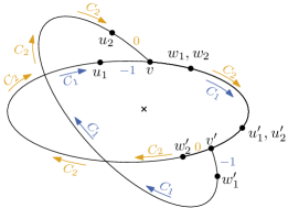
Figure 47: Illustration of proof for Lemma 27. It is assumed that the central face $g$ is neither the outer cascading cycle $C_{1}$ nor the increasing cycle $C_{1}$. Further, $C_{1}$ and $C_{2}$ have the edges $g[v,v^{\prime}]$ in common. It is proven that any edge of $C_{1}[v,v^{\prime}]$ has label $0$ and any edge of $C_{1}[v^{\prime},v]$ has label $-1$, which contradicts that $C_{1}$ is a cascading cycle.

Proof.

We assume without loss of generality that $C$ is an outer cascading cycle. The case that it is an inner cascading cycle can be handled by flipping the cylinder, which exchanges the exterior and interior of essential cycles but keeps the labels.

Let $g$ be the central face of the subgraph formed by the cycles $C_{1}$ and $C_{2}$. Assume that $g$ is neither $C_{1}$ nor $C_{2}$. Hence, there exist (not necessarily distinct) vertices $v$ and $v^{\prime}$ on $g$ such that $g[v,v^{\prime}]$ belongs to both $C_{1}$ and $C_{2}$, the edge that precedes $v$ on $g$ does not belong to $C_{2}$, and the edge that succeeds $v^{\prime}$ on $g$ does not belong to $C_{1}$; see Figure 47.

For $i=1,2$ let $u_{i}$ and $w_{i}$ be the vertices of $C_{i}$ that precede and succeed $v$, respectively. Further, let $u^{\prime}_{i}$ and $w^{\prime}_{i}$ be the vertices of $C_{i}$ that precede and succeed $v^{\prime}$, respectively. Since $u_{2}v$ strictly lies in the exterior of $g$, we obtain $\operatorname{rot}(u_{2}vw_{1})<\operatorname{rot}(u_{1}vw_{1})$. Hence, Lemma 8 gives $\ell_{C_{1}}(u_{1}v)<\ell_{C_{2}}(u_{2}v)$. Further, by definition of $C_{1}$ and $C_{2}$ it holds $\ell_{C_{1}}(u_{1}v)\geq-1$ and $\ell_{C_{2}}(u_{2}v)\leq 0$. Thus, we obtain $\ell_{C_{1}}(u_{1}v)=-1$ and $\ell_{C_{2}}(u_{2}v)=0$. Since $C_{1}$ is an outer cascading cycle this also implies that $v$ is the endpoint of the negative path $P$ of $C_{1}$.

Since $v^{\prime}w^{\prime}_{1}$ strictly lies in the exterior of $g$, we obtain $\operatorname{rot}(u^{\prime}_{2}v^{\prime}w^{\prime}_{2})>\operatorname{rot}(u^{\prime}_{2}v^{\prime}w^{\prime}_{1})$. Further, by the definition of labels we obtain $\ell_{C_{2}}(u^{\prime}_{2}v^{\prime})=\ell_{C_{2}}(v^{\prime}w^{\prime}_{2})-\operatorname{rot}(u^{\prime}_{2}v^{\prime}w^{\prime}_{2})$. Applying this in Lemma 8 gives $\ell_{C_{1}}(v^{\prime}w^{\prime}_{1})=\ell_{C_{2}}(v^{\prime}w^{\prime}_{2})-\operatorname{rot}(u^{\prime}_{2}v^{\prime}w^{\prime}_{2})+\operatorname{rot}(u^{\prime}_{2}v^{\prime}w^{\prime}_{1})$. Thus, we obtain $\ell_{C_{1}}(v^{\prime}w^{\prime}_{1})<\ell_{C_{2}}(v^{\prime}w^{\prime}_{2})$. Analogously to the arguments above, $\ell_{C_{2}}(v^{\prime}w^{\prime}_{2})=0$ and $\ell_{C_{1}}(v^{\prime}w^{\prime}_{1})=-1$. Thus, $v^{\prime}$ lies on $P$ and it is not the endpoint of $P$. It follows $v\neq v^{\prime}$ and $C_{1}-P$ is contained in $g[v,v^{\prime}]$. Hence, there is an edge $e$ on $g[v,v^{\prime}]$ with label $\ell_{C_{1}}(e)>0$. By Corollary 2 $\ell_{C_{2}}(e)=\ell_{C_{1}}(e)$, which contradicts that $C_{2}$ is an increasing cycle. ∎∎

We use the next lemma to show that the introduced paths $T$ and $B$ do not impact the validity of the ortho-radial representation.

Lemma 28.

Let $C$ be a cascading cycle in an ortho-radial representation $\Gamma$ and let $P$ be a sub-path of $C$ such that

1. the intermediate vertices of $P$ have degree 2 in the graph,

2. $P$ contains the negative path of $C$, and

3. $P$ contains an edge $e$ with label $\ell_{C}(e)>0$.

If $\Gamma$ without $P$ is valid, then $\Gamma$ is valid.

Proof.

First assume that $\Gamma$ contains a decreasing cycle $C^{\prime}$, which implies that $P$ is contained in $C^{\prime}$ (in either direction). Let $H=C+C^{\prime}$ be the common sub-graph of $C$ and $C^{\prime}$, and let $g$ be the central face of $H$. We distinguish the following two cases.

Case 1, $P$ is part of $g$. First assume that $C$ and $C^{\prime}$ use $P$ in opposite directions. Since the central face locally lies to the right of any essential cycle, this implies that the central face lies to the left and right of $P$. Consequently, the central face is not simple, which contradicts that $H$ is biconnected. So assume that $C$ and $C^{\prime}$ use $P$ in the same direction. By Proposition 8 it holds $\ell_{C}(e^{\prime})=\ell_{C^{\prime}}(e^{\prime})=-1$ for any edge $e^{\prime}$ on the negative path of $C$. Thus, $C^{\prime}$ is not a decreasing cycle.

Case 2, $P$ is not part of $g$. Let $C_{g}$ be the essential cycle formed by $g$. Since $C_{g}$ consists of edges of $C^{\prime}$ and $C$, the corresponding labels of $C^{\prime}$ and $C$ also apply on $C_{g}$ by Proposition 8. Further, since $C^{\prime}$ is a decreasing cycle and $P$ is the only part of $C$ that has a negative label on $C$, the cycle $C_{g}$ only has non-negative labels. Since $P$ does not lie on $C_{g}$ but on $C$, $C^{\prime}$ has at least one vertex with $C_{g}$ in common. By Proposition 1 the cycle $C_{g}$ is not horizontal. Altogether, $C_{g}$ is a decreasing cycle that also exists in $\Gamma-P$, which contradicts its validity.

Finally, assume that $\Gamma$ contains an increasing cycle $C^{\prime}$, which implies that $P$ is contained in $C^{\prime}$ in either direction. Lemma 27 implies that the central face $g$ of the subgraph formed by the two essential cycles $C$ and $C^{\prime}$ is either $C$ or $C^{\prime}$. In particular, $P$ or $\mkern 1.5mu\overline{\mkern-1.5muP\mkern-1.5mu}\mkern 1.5mu$ lies on $g$. Hence, both $C$ and $C^{\prime}$ use $P$ in the same direction as otherwise $g$ would lie in the exterior of one of these cycles. But this would contradict that they are essential. Hence, they both contain $P$ in this direction and $P$ also lies on $g$. By Proposition 8 both cycles have the same labels on $P$. Since $P$ contains the edge $e$ with $\ell_{C}(e)>0$ and thus $\ell_{C^{\prime}}(e)>0$, the cycle $C^{\prime}$ is not an increasing cycle. ∎∎

We construct a cascading cycle $C_{\mathrm{T}}$ in $\Gamma_{T}$ as follows. Let $C$ be the outermost decreasing cycle in $\Gamma^{u}_{e_{1}}$ and let $ut_{5}$ be the newly inserted edge in $\Gamma^{u}_{e_{1}}$. We replace $ut_{5}$ by $R[u,r_{4}]+T$ obtaining the cycle $C_{\mathrm{T}}$, which is well-defined because $C$ uses $ut_{5}$ in that direction by Lemma 20.

Lemma 29.

$C_{\mathrm{T}}$ is a cascading cycle with negative path $t_{1}t_{2}$ no matter whether $r_{2}r_{3}$ points to the right or downwards.

Proof.

Let $C$ be the outermost decreasing cycle in $\Gamma^{u}_{e_{1}}$. By Lemma 12 the labels of $C$ and $C_{\mathrm{T}}$ coincide on $C[t_{5},u](=C_{\mathrm{T}}[t_{5},u])$. Hence, since $C$ is a decreasing cycle all labels on $C_{\mathrm{T}}[t_{5},u]$ are non-negative. Further, by Lemma 20 the edge $ut_{5}$ has label $0$ on $C$. If $r_{2}r_{3}$ points to the right the sequence of the labels on $R[u,r_{4}]+T$ is therefore $0$, $0$, $0$, $-1$, $0$, $1$, $0$. If $r_{2}r_{3}$ points downwards the sequence is $0$, $1$, $0$, $-1$, $0$, $1$, $0$. In both cases $C_{\mathrm{T}}$ is a cascading cycle. ∎∎

Applying Lemma 27 to the situation of $C_{\mathrm{T}}$ proves that $\Gamma_{T}$ does not contain any increasing cycles. Together with Lemma 28 this yields that $\Gamma_{T}$ is valid. We analogously prove the validity of $\Gamma_{B}$ as for $\Gamma_{T}$. Let $C$ be the outermost decreasing cycle in $\Gamma^{u}_{e_{m-1}}$ and let $ub_{5}$ be the newly inserted edge in $\Gamma^{u}_{e_{m-1}}$. We replace $ub_{5}$ by $R[u,r_{5}]+B$ obtaining the cycle $C_{\mathrm{B}}$, which is well-defined because $C$ uses $ub_{5}$ in that direction by Lemma 20.

Lemma 30.

$C_{\mathrm{B}}$ is a cascading cycles no matter whether $r_{2}r_{3}$ points to the right or downwards. In particular, $b_{1}b_{2}$ is the negative path of $C_{\mathrm{B}}$.

Proof.

Let $C$ be the outermost decreasing cycle in $\Gamma^{u}_{e_{m-1}}$. By Lemma 12 the labels of $C$ and $C_{\mathrm{B}}$ coincide on $C[b_{5},u](=C_{\mathrm{B}}[b_{5},u])$. Hence, since $C$ is a decreasing cycle all labels on $C_{\mathrm{B}}[b_{5},u]$ are non-negative. Further, by Lemma 21 the edge $ub_{5}$ has label $0$ on $C$. If $r_{2}r_{3}$ points to the right the sequence of the labels on $R[u,r_{4}]+B$ is therefore $0$, $0$, $0$, $0$, $-1$, $0$, $1$, $0$. If $r_{2}r_{3}$ points downwards the sequence is $0$, $1$, $0$, $0$, $-1$, $0$, $1$, $0$. In both cases $C_{\mathrm{B}}$ is a cascading cycle. ∎∎

Applying Lemma 27 to the situation of $C_{\mathrm{T}}$ proves that $\Gamma_{B}$ does not contain any increasing cycles. Together with Lemma 28 this yields that $\Gamma_{B}$ is valid. The following lemma summarizes the result.

Lemma 31.

The ortho-radial representation $\Gamma_{B}=\Gamma_{1}$ is valid.

Correctness of Step 2.2.

By Lemma 31 the ortho-radial representation $\Gamma_{1}$ of Step 1 is valid. We now prove that $\Gamma_{2}$ is a valid ortho-radial representation. We use the same notation as in the description of the algorithm.

Starting with the valid ortho-radial representation $\Gamma_{1}$, the procedure iteratively resolves ports in the face $f_{1}$, which locally lies to the right of $T$. In case that we resolve a vertical port $u^{\prime}$ in a representation $\Pi$, the resulting ortho-radial representation $\Pi^{u^{\prime}}_{e^{\prime}_{1}}$ is valid by Fact 1 of Proposition 2, where $e^{\prime}_{1}$ is the first candidate of $u^{\prime}$. So assume that $u^{\prime}$ is a horizontal port. In that case we take $\Pi^{u^{\prime}}_{e^{\prime}_{l}}$ for the next iteration, where $e^{\prime}_{l}$ is the last candidate of $u^{\prime}$. We observe that the augmentation of $f_{1}$ may subdivide edges on the negative paths of $C_{\mathrm{T}}$ and $C_{\mathrm{B}}$, but the added edges lie in the interior of $C_{\mathrm{T}}$ and the exterior of $C_{\mathrm{B}}$. Hence, $C_{\mathrm{T}}$ remains an outer cascading cycle and $C_{\mathrm{B}}$ an inner cascading cycle.

Lemma 32.

The ortho-radial representation $\Pi^{u^{\prime}}_{e^{\prime}_{l}}$ is valid.

Proof.

Assume that $\Pi^{u^{\prime}}_{e^{\prime}_{l}}$ is not valid. Hence, there is a strictly monotone cycle $C$ that uses $e=u^{\prime}z^{\prime}$, where $z^{\prime}$ is the vertex subdividing $e^{\prime}_{l}$. Since $e^{\prime}_{l}$ is the last candidate of $u^{\prime}$, the cycle $C$ is increasing by Fact 2 of Proposition 2. By construction $e$ strictly lies in the interior of $C_{\mathrm{T}}$ and the exterior of $C_{\mathrm{B}}$. This implies that $C$ lies in the interior of $C_{\mathrm{T}}$ and the exterior of $C_{\mathrm{B}}$ by Lemma 27. In other words, $C$ is contained in the subgraph $H$ formed by the intersection of the interior of $C_{\mathrm{T}}$ and the exterior of $C_{\mathrm{B}}$. As $R[r_{1},r_{4}]$ belongs to both $C_{\mathrm{T}}$ and $C_{\mathrm{B}}$, it is incident to the outer and the central face of $H$. Hence, removing $R[r_{1},r_{4}]$ leaves a subgraph without essential cycles. Thus, the essential cycle $C$ includes $R[r_{1},r_{4}]$.

By Proposition 8 the labels of $C$ and $C_{\mathrm{T}}$ are the same on $R[r_{1},r_{4}]$. If $r_{2}r_{3}$ points downwards, its label is $1$, which contradicts that $C$ is increasing. If otherwise $r_{2}r_{3}$ points right, it lies on a horizontal cycle. But then $C$ is not increasing by Proposition 1. ∎∎

Altogether, applying the lemma inductively on the inserted edges, we obtain that $\Gamma_{2}$ is valid.

Correctness of Step 2.3.

As we only apply the first phase of the augmentation step on $f_{2}$, the resulting ortho-radial representation $\Gamma_{3}$ is also valid due to the correctness of the first phase. This concludes the correctness proof of the second phase.

10 Bend Minimization

We have considered bend-free ortho-radial drawings so far. In this section we shortly describe how to extend our results to ortho-radial drawings with bends. In particular, we present complexity results on bend-minimzation for ortho-radial drawings.

We model bends by subdividing each edge of $G$ with $K$ degree-2 vertices. Let $S$ denote the set of all these subdivision vertices. A vertex $v\in S$ is a bend in an ortho-radial representation if for its two incident edges $e_{1}$ and $e_{2}$ it holds $\operatorname{rot}(e_{1},e_{2})\neq 0$. A valid ortho-radial representation of $I$ is bend-minimal if there is no other valid ortho-radial representation of $I$ that has fewer bends. Niedermann and Rutter [27] recently showed that $K=2n-4$ subdivision vertices per edge are sufficient for creating bend-minimal valid ortho-radial representations. The next theorem shows that from a computational point of view there is a substantial difference between creating orthogonal drawings and ortho-radial drawings with a minimum number of bends even if the embedding is prescribed.

Theorem 4.

Given an instance $I=(G,\mathcal{E},f_{c},f_{o})$, finding a bend-minimal valid ortho-radial representation of $I$ is $\mathcal{NP}$-hard.

Proof.

Given a valid bend-minimal ortho-radial representation $\Gamma$, we utilize the TSM framework to create a bend-minimal ortho-radial drawing $\Delta$ based on $\Gamma$ in polynomial time. Consequently, if $\Gamma$ could be created in polynomial time, we could also derive $\Delta$ in polynomial time. On the other hand, Garrido and Marquez [20] proved that given an embedding $\mathcal{E}$ of a graph $G$ in a surface $S$ with genus $g$ it is $\mathcal{NP}$-hard to find an orthogonal grid drawing of $\mathcal{E}$ on $S$ that minimizes the number of bends. In particular, for $g=0$ the surface $S$ corresponds to a sphere. As the constructions used in the proposed reduction from 3SAT do not use the poles of the sphere, this result directly transfers to orthogonal grid drawings on cylinders and hence to ortho-radial drawings. ∎∎

Niedermann and Rutter [27] recently presented an integer linear programming formulation for creating valid bend-minimal ortho-radial representations assuming a pre-defined embedding of the graph.

If we do not assume a pre-defined embedding of the graph, finding a bend-minimal drawing becomes $\mathcal{NP}$-hard even for the orthogonal case. Garg and Tamassia [19] showed that the problem Orthogonal Embeddability to decide whether a given planar 4-graph admits an orthogonal drawing without bends is $\mathcal{NP}$-complete. In the remaining part of this section we study the analogous problem Ortho-radial Embeddability for ortho-radial drawings and prove that it is $\mathcal{NP}$-complete as well. We say a graph $G$ admits an ortho-radial (or orthogonal) embedding if there is an embedding of $G$ such that $G$ can be drawn ortho-radially (or orthogonally) without bends.

We give a reduction from Orthogonal Embeddability. To do so, we note that the reduction by Garg and Tamassia [19] actually produces instances $G=(V,E)$ with a fixed edge $e\in E$ such that it is $\mathcal{NP}$-complete to decide whether $G$ has an orthogonal embedding where $e$ is incident to the outer face.

Given such a graph, we build a structure around $G$ that yields a graph $G^{\prime}$ such that in any ortho-radial embedding of $G^{\prime}$ the induced representation $\Gamma$ of $G$ does not contain any essential cycles. In other words, $\Gamma$ is actually an orthogonal representation of $G$. Hence, an ortho-radial embedding of $G^{\prime}$ can only exist if $G$ admits an orthogonal embedding. We may assume without loss of generality that $G$ is connected as otherwise, we handle each component separately.

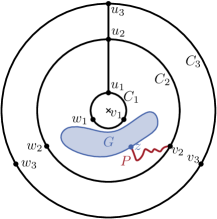
(a) $G$ lies between $C_{1}$ and $C_{2}$.

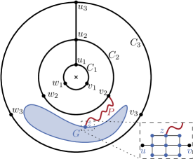
(b) $G$ lies between $C_{2}$ and $C_{3}$.

Figure 48: Possible embeddings of $G^{\prime}$: In both cases $G$ contains no essential cycles. The roles of $C_{1}$ and $C_{3}$ can be exchanged.

The construction of $G^{\prime}$ from $G$ is based on the fact that there is only one way to ortho-radially draw a triangle $C$, i.e., a cycle of length 3, without bends: as an essential cycle on one circle of the grid. We build a graph $H$ consisting of three triangles called $C_{1}$, $C_{2}$ and $C_{3}$ and denote the vertices on $C_{i}$ by $u_{i}$, $v_{i}$ and $w_{i}$. Furthermore, $H$ contains the edges $u_{1}u_{2}$ and $u_{2}u_{3}$. In Figure 48 $H$ is formed by the black edges. To connect $H$ and $G$, we replace the special edge $e=uv$ of $G$ by a $3\times 3$-grid and connect one of the degree-3 vertices $z$ of that grid by a path $P$ to $v_{2}$, where we choose the length of the path equal to the number of edges in $G$. The resulting graph is $G^{\prime}$; see Figure 48. The reduction clearly runs in polynomial time. Moreover, if $G^{\prime}$ admits an ortho-radial embedding, then the triangles of $H$ must be drawn as essential cycles, and therefore $G$ must be contained in one of the two regular faces of $H$, and can hence not contain any essential cycles. We therefore find an orthogonal embedding of $G$. Conversely, if we have an orthogonal embedding of $G$ with $e$ on the outer face, then it can be inserted into a face of the drawing of $H$ and the path $P$ can be drawn as it is sufficiently long. We therefore obtain an ortho-radial embedding of $G^{\prime}$. This proves the following theorem.

Theorem 5.

Ortho-radial Embeddability is $\mathcal{NP}$-complete.

11 Conclusion

In this paper we considered orthogonal drawings of graphs on cylinders. Our main result is a characterization of the plane 4-graphs that can be drawn bend-free on a cylinder in terms of a combinatorial description of such drawings. These ortho-radial representations determine all angles in the drawing without fixing any lengths, and thus are a natural extension of Tamassia’s orthogonal representations. However, compared to those, the proof that every valid ortho-radial representation has a corresponding drawing is significantly more involved. The reason for this is the more global nature of the additional property required to deal with the cyclic dimension of the cylinder.

Our ortho-radial representations establish the existence of an ortho-radial TSM framework in the sense that they are a combinatiorial description of the graph serving as interface between the “Shape” and “Metrics” step.

For rectangular plane 4-graphs, we gave an algorithm producing a drawing from a valid ortho-radial representation. Our proof reducing the drawing of general plane 4-graphs with a valid ortho-radial representation to the case of rectangular plane 4-graphs is constructive. We have described an algorithm that checks the validity of an ortho-radial representation in $\mathcal{O}(n^{2})$ time. In the positive case, we can also produce a corresponding drawing in the same running time, whereas in the negative case we find a strictly monotone cycle. These algorithms correspond to the “Metrics” step in a TSM framework for ortho-radial drawings.

While bend-minimal orthogonal representations can be created in polynomial time, we showed that creating valid bend-minimal ortho-radial representations is $\mathcal{NP}$-hard. This directly rises the research question of developing approximation algorithms and fixed parameter tractable algorithms for such representations. Further, powerful and fast heuristics may help to carry over the framework into practice, e.g., for creating ortho-radial drawings of large transportation networks.

Finally, we want to emphasize that we deem the generalization of ortho-radial drawings from the cylinder to the torus or even more complex surfaces an interesting and promising research question. It is far from clear how to transfer our results to the torus as its two cyclic dimensions lead to different types of essential cycles.

Acknowledgments

Lukas Barth was funded by the German Research Foundation (DFG) as part of the Research Training Group GRK 2153: Energy Status Data – Informatics Methods for its Collection, Analysis and Exploitation. Matthias Wolf was funded by the Helmholtz Association Program Storage and Cross-linked Infrastructures, Topic 6 Superconductivity, Networks and System Integration and by the German Research Foundation (DFG) as part of the Research Training Group GRK 2153: Energy Status Data – Informatics Methods for its Collection, Analysis and Exploitation.

References

- [1] Alam, M.J., Kobourov, S.G., Mondal, D.: Orthogonal layout with optimal face complexity. Computational Geometry 63, 40–52 (2017)
- [2] Batini, C., Nardelli, E., Tamassia, R.: A layout algorithm for data flow diagrams. IEEE Transactions on Software Engineering SE-12(4), 538–546 (1986)
- [3] Bertolazzi, P., Battista, G.D., Didimo, W.: Computing orthogonal drawings with the minimum number of bends. IEEE Transactions on Computers 49(8), 826–840 (2000)
- [4] Bhatt, S.N., Leighton, F.T.: A framework for solving VLSI graph layout problems. Journal of Computer and System Sciences 28(2), 300–343 (1984)
- [5] Biedl, T.: New lower bounds for orthogonal graph drawings. In: F.J. Brandenburg (ed.) Graph Drawing (GD’96), Lecture Notes of Computer Science, pp. 28–39. Springer Berlin Heidelberg (1996)
- [6] Biedl, T., Kant, G.: A better heuristic for orthogonal graph drawings. Computational Geometry 9(3), 159 – 180 (1998)
- [7] Biedl, T.C., Madden, B.P., Tollis, I.G.: The three-phase method: A unified approach to orthogonal graph drawing. In: G. DiBattista (ed.) Graph Drawing (GD’97), Lecture Notes in Computer Science, pp. 391–402. Springer Berlin Heidelberg (1997)
- [8] Bläsius, T., Rutter, I., Wagner, D.: Optimal orthogonal graph drawing with convex bend costs. ACM Transactions on Algorithms 12(3), 33 (2016)
- [9] Bläsius, T., Lehmann, S., Rutter, I.: Orthogonal graph drawing with inflexible edges. Computational Geometry 55, 26 – 40 (2016)
- [10] Chang, Y.J., Yen, H.C.: On bend-minimized orthogonal drawings of planar 3-graphs. In: B. Aronov, M.J. Katz (eds.) Computational Geometry (SoCG’17), Leibniz International Proceedings in Informatics (LIPIcs), vol. 77. Schloss Dagstuhl-Leibniz-Zentrum fuer Informatik (2017)
- [11] Cornelsen, S., Karrenbauer, A.: Accelerated bend minimization. In: M. van Kreveld, B. Speckmann (eds.) Graph Drawing (GD’12), Lecture Notes of Computer Science, pp. 111–122. Springer Berlin Heidelberg (2012)
- [12] Di Battista, G., Eades, P., Tamassia, R., Tollis, I.G.: Graph Drawing - Algorithms for the Visualization of Graphs. Prentice Hall (1999)
- [13] Eiglsperger, M., Gutwenger, C., Kaufmann, M., Kupke, J., Jünger, M., Leipert, S., Klein, K., Mutzel, P., Siebenhaller, M.: Automatic layout of uml class diagrams in orthogonal style. Information Visualization 3(3), 189–208 (2004)
- [14] Eiglsperger, M., Kaufmann, M., Siebenhaller, M.: A topology-shape-metrics approach for the automatic layout of uml class diagrams. In: Software Visualization (SoftVis’03), pp. 189–ff. ACM (2003)
- [15] Felsner, S., Kaufmann, M., Valtr, P.: Bend-optimal orthogonal graph drawing in the general position model. Computational Geometry 47(3, Part B), 460–468 (2014). Special Issue on the 28th European Workshop on Computational Geometry (EuroCG 2012)
- [16] Fink, M., Haverkort, H., Nöllenburg, M., Roberts, M., Schuhmann, J., Wolff, A.: Drawing metro maps using bézier curves. In: W. Didimo, M. Patrignani (eds.) Graph Drawing (GD’13), Lecture Notes in Computer Science, pp. 463–474. Springer International Publishing (2013)
- [17] Fink, M., Lechner, M., Wolff, A.: Concentric metro maps. In: Abstracts of the Schematic Mapping Workshop 2014 (2014)
- [18] Fößmeier, U., Kaufmann, M.: Drawing high degree graphs with low bend numbers. In: F.J. Brandenburg (ed.) Graph Drawing (GD’96), Lecture Notes in Computer Science, pp. 254–266. Springer Berlin Heidelberg (1996)
- [19] Garg, A., Tamassia, R.: On the computational complexity of upward and rectilinear planarity testing. SIAM Journal on Computing 31(2), 601–625 (2001)
- [20] Garrido, M.A., Márquez, A.: Embedding a graph in the grid of a surface with the minimum number of bends is np-hard. In: G. DiBattista (ed.) Graph Drawing, pp. 124–133. Springer Berlin Heidelberg, Berlin, Heidelberg (1997)
- [21] Gutwenger, C., Jünger, M., Klein, K., Kupke, J., Leipert, S., Mutzel, P.: A new approach for visualizing UML class diagrams. In: Symposium on Software Visualization (SoftVis’03), pp. 179–188. ACM, New York, NY, USA (2003)
- [22] Hasheminezhad, M., Hashemi, S.M., McKay, B.D., Tahmasbi, M.: Rectangular-radial drawings of cubic plane graphs. Computational Geometry: Theory and Applications 43, 767–780 (2010)
- [23] Hasheminezhad, M., Hashemi, S.M., Tahmabasi, M.: Ortho-radial drawings of graphs. Australasian Journal of Combinatorics 44, 171–182 (2009)
- [24] Hong, S.H., Merrick, D., do Nascimento, H.A.D.: Automatic visualisation of metro maps. Journal of Visual Languages and Computing 17(3), 203–224 (2006)
- [25] Kieffer, S., Dwyer, T., Marriott, K., Wybrow, M.: Hola: Human-like orthogonal network layout. IEEE Transactions on Visualization and Computer Graphics 22(1), 349–358 (2016)
- [26] Miller, G.L., Naor, J.: Flow in planar graphs with multiple sources and sinks. SIAM J. Comput. 24(5), 1002–1017 (1995). DOI 10.1137/S0097539789162997
- [27] Niedermann, B., Rutter, I.: An Integer-Linear Program for Bend-Minimization in Ortho-Radial Drawings. In: D. Auber, P. Valtr (eds.) Graph Drawing and Network Visualization (GD’20), Lecture Notes in Computer Science. Springer (2020). To appear.
- [28] Nöllenburg, M., Wolff, A.: Drawing and labeling high-quality metro maps by mixed-integer programming. Transactions on Visualization and Computer Graphics 17(5), 626–641 (2011)
- [29] Papakostas, A., Tollis, I.G.: Algorithms for area-efficient orthogonal drawings. Computational Geometry 9(1), 83–110 (1998)
- [30] Rüegg, U., Kieffer, S., Dwyer, T., Marriott, K., Wybrow, M.: Stress-minimizing orthogonal layout of data flow diagrams with ports. In: C. Duncan, A. Symvonis (eds.) Graph Drawing (GD’14), Lecture Notes in Computer Science, pp. 319–330. Springer Berlin Heidelberg (2014)
- [31] Tamassia, R.: On embedding a graph in the grid with the minimum number of bends. SIAM Journal on Computing 16(3), 421–444 (1987)
- [32] Tamassia, R., Di Battista, G., Batini, C.: Automatic graph drawing and readability of diagrams. IEEE Transactions on Systems, Man, and Cybernetics 18(1), 61–79 (1988)
- [33] Tamassia, R., Tollis, I.G., Vitter, J.S.: Lower bounds for planar orthogonal drawings of graphs. Information Processing Letters 39(1), 35 – 40 (1991)
- [34] Valiant, L.G.: Universality considerations in vlsi circuits. IEEE Transactions on Computers 30(02), 135–140 (1981)
- [35] Wang, Y.S., Chi, M.T.: Focus+context metro maps. Transactions on Visualization and Computer Graphics 17(12), 2528–2535 (2011)
- [36] Wybrow, M., Marriott, K., Stuckey, P.J.: Orthogonal connector routing. In: D. Eppstein, E.R. Gansner (eds.) Graph Drawing (GD’10), Lecture Notes in Computer Science, pp. 219–231. Springer Berlin Heidelberg (2010)