Cooperative Multi-Agent Fairness and Equivariant Policies

Abstract

We study fairness through the lens of cooperative multi-agent learning. Our work is motivated by empirical evidence that naive maximization of team reward yields unfair outcomes for individual team members. To address fairness in multi-agent contexts, we introduce team fairness, a group-based fairness measure for multi-agent learning. We then prove that it is possible to enforce team fairness during policy optimization by transforming the team’s joint policy into an equivariant map. We refer to our multi-agent learning strategy as Fairness through Equivariance (Fair-E) and demonstrate its effectiveness empirically. We then introduce Fairness through Equivariance Regularization (Fair-ER) as a soft-constraint version of Fair-E and show that it reaches higher levels of utility than Fair-E and fairer outcomes than non-equivariant policies. Finally, we present novel findings regarding the fairness-utility trade-off in multi-agent settings; showing that the magnitude of the trade-off is dependent on agent skill.

1 Introduction

Algorithmic fairness is an increasingly important sub-domain of AI. As statistical learning algorithms continue to automate decision-making in crucial areas such as lending (Fuster et al. 2020), healthcare (Potash et al. 2015), and education (Dorans and Cook 2016), it is imperative that the performance of such algorithms does not rely upon sensitive information pertaining to the individuals for which decisions are made (e.g. race, gender). Despite its growing importance, fairness research has largely targeted prediction-based problems, where decisions are made for one individual at one time (Mitchell et al. 2018). Though recent studies have extended fairness to the multi-agent case (Jiang and Lu 2019), such work primarily considers social dilemmas in which team utility is in obvious conflict with the local interests of each team member (Leibo et al. 2017; Rapoport 1974; Van Lange et al. 2013).

Many real-world problems, however, must weigh the fairness implications of team behavior in the presence of a single overarching goal. In-line with recent work that has highlighted the importance of leveraging multi-agent learning to study socio-economic challenges such as taxation, social planning, and economic policy (Zheng et al. 2020), we posit that understanding the range of team behavior that emerges from single-objective utility maximization is crucial for the development of fair multi-agent systems. For this reason, we study fairness in the context of cooperative multi-agent settings. Cooperative multi-agent fairness differs from traditional game-theoretic interpretations of fairness (e.g. resource allocation (Elzayn et al. 2019; Zhang and Shah 2014), social dilemmas (Leibo et al. 2017)) in that it seeks to understand the fairness implications of emergent coordination learned by multi-agent teams that are bound by a shared reward. Cooperative multi-agent fairness therefore reframes the question—“Will agents cooperate or defect, given the choice between local and team interests?”—to a related but novel question—“Given the incentive to work together, do agents learn to coordinate effectively and fairly?”

Experimentally, we target pursuit-evasion (i.e. predator-prey) as a test-bed for cooperative multi-agent fairness. Pursuit-evasion allows us to simulate a number of important components of socio-economic systems, including: (i) Shared objectives: the overarching goal of pursuers is to capture an evader; (ii) Agent skill: the speed of the pursuers relative the evader serves as a proxy for skill; (iii) Coordination: success requires sophisticated cooperation by the pursuers. Using pursuit-evasion, we study the fairness implications of behavior that emerges under variations of these “socio-economic” parameters. Similar to prior work (Lowe et al. 2017; Mordatch and Abbeel 2018; Grupen, Lee, and Selman 2020), we cast pursuit-evasion as a multi-agent reinforcement learning (RL) problem.

Our first result highlights the importance of shared objectives to cooperation. In particular, we compare policies learned when pursuers share in team success (mutual reward) to those learned when pursuers do not share reward (individual reward). We find that sophisticated coordination only emerges when pursuers are bound by mutual reward. Given individual reward, pursuers are not properly incentivized to work together. However, though mutual reward aides coordination, it does not specify how to coordinate fairly. In our experiments, we find that naive, unconstrained maximization of mutual reward yields unfair individual outcomes for cooperative teammates. In the context of pursuit-evasion, the optimal strategy is a form of role assignment—the majority of pursuers act as supporting agents, shepherding the evader to one designated “capturer” agent. Solving this issue is the subject of the rest of our analysis.

Addressing this form of unfair emergent coordination requires connecting fairness to multi-agent learning settings. To do this, we first introduce team fairness, a group-based fairness measure inspired by demographic parity (Dwork et al. 2012; Feldman et al. 2015). Team fairness requires the distribution of a team’s reward to be equitable across sensitive groups. We then show that it is possible to enforce team fairness during policy optimization by transforming the team’s joint policy into an equivariant map. We prove that equivariant policies yield fair reward distributions under assumptions of agent homogeneity. We refer to our multi-agent learning strategy as Fairness through Equivariance (Fair-E) and demonstrate its effectiveness empirically in pursuit-evasion experiments.

Despite achieving fair outcomes, Fair-E represents a binary switch—one can either choose fairness (at the expense of utility) or utility (at the expense of fairness). In many cases, however, it is advantageous to modulate between fairness and utility. To this end, we introduce a soft-constraint version of Fair-E that incentivizes equivariance through regularization. We refer to this method as Fairness through Equivariance Regularization (Fair-ER) and show that it is possible to tune fairness constraints over multi-agent policies by adjusting the weight of equivariance regularization. Moreover, we show empirically that Fair-ER reaches higher levels of utility than Fair-E while achieving fairer outcomes than non-equivariant policy learning.

Finally, as in both prediction-based settings (Corbett-Davies et al. 2017; Zhao and Gordon 2019) and in traditional multi-agent variants of fairness (Okun 1975; Le Grand 1990), it is important to understand the “cost” of fairness. We present novel findings regarding the fairness-utility trade-off for cooperative multi-agent settings. Specifically, we show that the magnitude of the trade-off depends on the skill level of the multi-agent team. When agent skill is high (making the task easier to solve), fairness comes with no trade-off in utility, but as skill decreases (making the task more difficult), gains in team fairness are increasingly offset by decreases in team utility.

Preview of contributions In sum, our work offers the following contributions:

• We show that mutual reward is critical to multi-agent coordination. In pursuit-evasion, agents trained with mutual reward learn to coordinate effectively, whereas agents trained with individual reward do not.

• We connect fairness to cooperative multi-agent settings. We introduce team fairness as a group-based fairness measure for multi-agent teams that requires equitable reward distributions across sensitive groups.

• We introduce Fairness through Equivariance (Fair-E), a novel multi-agent strategy leveraging equivariant policy learning. We prove that Fair-E achieves fair outcomes for individual members of a cooperative team.

• We introduce Fairness through Equivariance Regularization (Fair-ER) as a soft-constraint version of Fair-E. We show that Fair-ER reaches higher levels of utility than Fair-E while achieving fairer outcomes than non-equivariant learning.

• We present novel findings regarding the fairness-utility trade-off for cooperative settings. Specifically, we show that the magnitude of the trade-off depends on agent skill—when agent skill is high, fairness comes for free; whereas with lower skill levels, fairness is increasingly expensive.

2 Related work

At a high-level, the prediction-based fairness literature can be split into two factions: individual fairness and group fairness. Introduced by Dwork et al. (2012), individual fairness posits that two individuals with similar features should be classified similarly (i.e. similarity in feature-space implies similarity in decision-space). Such approaches rely on task-specific distance metrics with which similarity can be measured (Barocas, Hardt, and Narayanan 2019; Chouldechova and Roth 2018). Group fairness, on the other hand, attempts to achieve outcome consistency across sensitive groups. This idea has given rise to a number of methods such as statistical/demographic parity (Feldman et al. 2015; Johndrow, Lum et al. 2019; Kamiran and Calders 2009; Zafar et al. 2017), equality of opportunity (Hardt, Price, and Srebro 2016), and calibration (Kleinberg, Mullainathan, and Raghavan 2016). Recent work has extended fairness to the RL setting to consider the feedback effects of decision-making (Jabbari et al. 2017; Wen, Bastani, and Topcu 2021).

In multi-agent systems, fairness is typically studied in game-theoretic settings in which individual payoffs and overall group utility are in obvious conflict (De Jong et al. 2005, 2007)—such as resource allocation (Elzayn et al. 2019; Zhang and Shah 2014) and social dilemmas (Leibo et al. 2017; Rapoport 1974; Van Lange et al. 2013). In multi-agent RL settings, these tensions have been addressed through myriad techniques, including reward shaping (Peysakhovich and Lerer 2017), intrinsic reward (Wang et al. 2018), parameterized inequity aversion (Hughes et al. 2018), and hierarchical learning (Jiang and Lu 2019). Also related is the Shapley value: a method for sharing surplus across a coalition based on one’s contributions to the coalition (Shapley 2016). Shapley value-based credit assignment techniques have recently been shown to stabilize learning and achieve fairer outcomes when incorporated into the multi-agent RL problem (Wang et al. 2020; Li et al. 2021).

Our work differs from this prior work in two key ways. First we target fully-cooperative multi-agent settings (Hao and Leung 2016) in which fairness implications emerge naturally in the presence of a single overarching goal (i.e. mutual reward). In this fully-cooperative setting, individual and team incentives are not in obvious conflict. Our motivation for studying fully-cooperative team objectives follows from recent work that highlights the role of multi-agent learning in real-world problems characterized by shared objectives, including taxation and economic policy (Zheng et al. 2020). Moreover, we study modifications to the utility-maximization objective that yield fairer outcomes by incentivizing agents to change their behavior, rather than redistributing outcomes after-the-fact. Most relevant is Siddique, Weng, and Zimmer (2020) and Zimmer, Siddique, and Weng (2020), which introduce a class of algorithms that successfully achieve fair outcomes for multi-agent teams through pre-defined social welfare functions that encode specific fairness principles. Our work, conversely, introduces task-agnostic methods for incentivizing fairness through both hard-constraints on agent policies and soft-constraints (i.e. regularization) (Liu et al. 2018) on the RL objective.

Finally, discussion of the fairness-utility (or fairness-efficiency) trade-off has a long history in game-theoretic multi-agent settings (Okun 1975; Le Grand 1990; Bertsimas, Farias, and Trichakis 2012; Joe-Wong et al. 2013; Bertsimas, Farias, and Trichakis 2011) and is also prevalent throughout the prediction-based fairness literature (Menon and Williamson 2018). Existing work has shown both theoretically (Calders, Kamiran, and Pechenizkiy 2009; Kleinberg, Mullainathan, and Raghavan 2016; Zhao and Gordon 2019) and empirically (Dwork et al. 2012; Feldman et al. 2015; Kamiran and Calders 2009; Lahoti, Gummadi, and Weikum 2019; Pannekoek and Spigler 2021) that gains in fairness come at the cost of utility. Our discussion of the fairness-utility trade-off is most similar to Corbett-Davies et al. (2017) in this regard, as we study the trade-off through the lens of constrained vs. unconstrained optimization. However, we take this trade-off a step further, outlining a relationship between fairness, utility, and agent skill that is not present in prior work.

3 Preliminaries

Markov games

A Markov game is a multi-agent extension of the Markov decision process (MDP) formalism (Littman 1994). For $n$ agents, it is represented by a state space $\mathcal{S}$, joint action space $\boldsymbol{\mathcal{A}}=\{\mathcal{A}_{1},...,\mathcal{A}_{n}\}$, joint observation space $\boldsymbol{\mathcal{O}}=\{\mathcal{O}_{1},...,\mathcal{O}_{n}\}$, transition function $\mathcal{T}:\mathcal{S}\times\boldsymbol{\mathcal{A}}\rightarrow\mathcal{S}$, and joint reward function $\boldsymbol{r}$. Following multi-objective RL (Zimmer, Siddique, and Weng 2020), we define a vectorial reward $\boldsymbol{r}:\mathcal{S}\times\boldsymbol{\mathcal{A}}\rightarrow\mathbb{R}^{n}$ with each component $r_{i}$ representing agent $i$’s contribution to $\boldsymbol{r}$. Each agent $i$ is initialized with a policy $\pi_{i}:\mathcal{O}_{i}\rightarrow\mathcal{A}$ (or deterministic policy $\mu_{i}$) from which it selects actions and an action-value function $Q_{i}:\mathcal{S}\times\mathcal{A}_{i}\rightarrow\mathbb{R}$ with which it judges the value of state-action pairs. Following action selection, the environment transitions from its current state $s_{t}$ to a new state $s_{t+1}$, as governed by $\mathcal{T}$, and produces a reward vector $\boldsymbol{r}_{t}$ indicating the strength or weakness of the group’s decision-making. In the episodic case, this process continues for a finite time horizon $T$, producing a trajectory $\tau=(s_{1},\boldsymbol{a_{1}},...,s_{T-1},\boldsymbol{a_{T-1}},s_{T})$ with probability:

$$P(\tau)=P_{\emptyset}(s_{1})\prod_{t=1}^{T}P(s_{t+1}|s_{t},a_{t})\pi(a_{t}|s_{t})$$ (1)

where $P_{\emptyset}$ is a special distribution specifying the likelihood of each “start” state.

Deep deterministic policy gradients

Deep Deterministic Policy Gradients (DDPG) is an off-policy actor-critic algorithm for policy gradient learning in continuous action spaces (Lillicrap et al. 2015). DDPG leverages the deterministic policy gradient theorem (Silver et al. 2014), which asserts that it is possible to find an optimal deterministic policy ($\mu_{\phi}$, with parameters $\phi$), with respect to a Q-function ($Q_{\omega}$, with parameters $\omega$), for the RL objective:

$$J(\phi)=\mathbb{E}_{s}[Q_{\omega}(s,a)|_{s=s_{t},a=\mu_{\phi}(s_{t})}]$$ (2)

by performing gradient ascent with respect to the following gradient:

$$\nabla_{\phi}J(\phi)=\mathbb{E}_{s}[\nabla_{a}Q_{\omega}(s,a)|_{s=s_{t},a=\mu(s_{t})}\nabla_{\phi}\mu(s)|_{s=s_{t}}]$$ (3)

under mild conditions that confirm the existence of gradients $\nabla_{a}Q_{\omega}(s,a)$ and $\nabla_{\phi}\mu(s)$. For critic updates, DDPG follows batched TD-control, where the Q-function minimizes the loss function:

$$L(\omega)=\underset{s,a,r,s^{\prime}}{\mathbb{E}}\big{[}\big{(}Q_{\omega}(s,a)-(r(s,a)+\gamma Q_{\omega}(s^{\prime},\mu_{\phi}(s^{\prime})))\big{)}^{2}\big{]}$$ (4)

where ($s,a,r,s^{\prime}$) are transition tuples sampled from a replay buffer. In this work, agents learn in a decentralized manner, each performing DDPG updates individually.

Fairness

Prediction-based fairness considers a population of $n$ individuals (indexed $i=1,...,n$), each described by variables $v_{i}$ (i.e. features or attributes), which are separated into sensitive variables $z_{i}$ and other variables $x_{i}$. Variables $v_{i}$ are used to predict (typically binary) outcomes $y_{i}\in Y$ by estimating the conditional probability $P[Y=1|V=v_{i}]$ through a scoring function $\psi:\mathcal{V}\rightarrow\{0,1\}$. Outcomes in turn yield decisions by applying a decision rule $\delta(v_{i})=f(\psi(v_{i}))$. For example, in a lending scenario, a classifier may use $v_{i}$ to predict whether an individual $i$ will default on ($y_{i}=0$) or repay ($y_{i}=1$) his/her loan, which informs the decision to deny ($d_{i}=0$) or approve ($d_{i}=1$) the individual’s loan application (Mitchell et al. 2018). Of particular relevance is group-based fairness, which examines how well outcome ($Y$) and decision ($D$) consistency is preserved across sensitive groups ($Z$) (Feldman et al. 2015; Zafar et al. 2017). We highlight the group-based measure of demographic parity, which requires that $D\perp Z$ or, equivalently, that $P[D=1|Z=z]=P[D=1|Z=z^{\prime}]$ for all $z,z^{\prime}$ where $z\neq z^{\prime}$.

Mutual Information

Given random variables $X_{1}{\sim}P_{X_{1}}$ and $X_{2}{\sim}P_{X_{2}}$ with joint distribution $P_{X_{1}X_{2}}$, mutual information is defined as the Kullback-Leibler (KL-) divergence between the joint $P_{X_{1}X_{2}}$ and the product of the marginals $P_{X_{1}}\otimes P_{X_{2}}$:

$$I(X_{1};X_{2}):=D_{KL}(P_{X_{1}X_{2}}||P_{X_{1}}\otimes P_{X_{2}})\\$$ (5)

Mutual information quantifies the dependence between $X_{1}$ and $X_{2}$ where, in Equation 5, larger divergence represents stronger dependence. Importantly, mutual information can also be represented as the decrease in entropy of $X_{1}$ when introducing $X_{2}$:

$$I(X_{1};X_{2}):=H(X_{1})-H(X_{1}|X_{2})$$ (6)

Equivariance

Let $g_{1}$ and $g_{2}$ be G-sets of a group $G$ and $\sigma$ be a symmetry transformation over $G$. Then a function $f:g_{1}\rightarrow g_{2}$ is equivariant with respect to $\sigma$ if the commutative relationship $f(\sigma\cdot x)=\sigma\cdot f(x)$ holds. Equivariance in the context of RL implies that separate policies will take the same actions under permutations of state space.

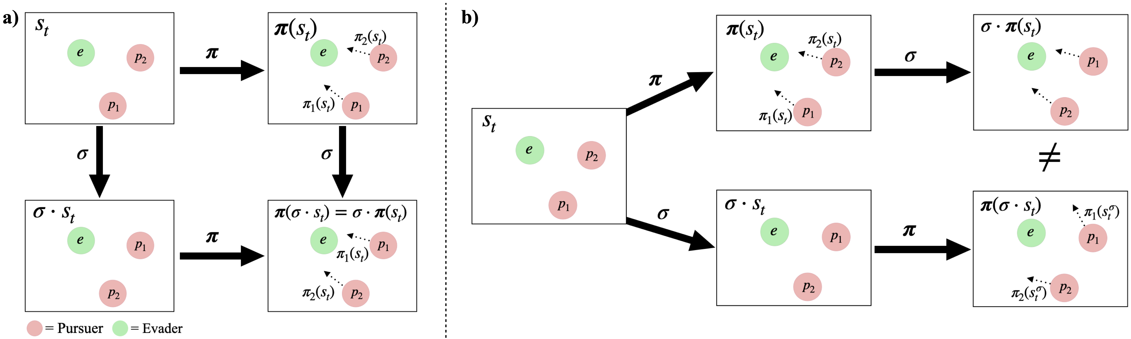
Figure 1: Snapshot of a pursuit-evasion game. Pursuers $p_{1}$ and $p_{2}$ (red) chase an evader $e$ (green) with the goal of capturing it. Given a state $s_{t}$, each pursuer selects its next heading (dotted arrow) from its policy, yielding the joint policy $\boldsymbol{\pi}{=}\{\pi_{1}(s_{t}),\pi_{2}(s_{t})\}$. Evader action selection is omitted for clarity. a) For an equivariant joint policy, applying the transformation $\sigma$ to the state $s_{t}$ (producing $\sigma\cdot s_{t}$ which, in this example, swaps the positions of $p_{1}$ and $p_{2}$) and running the policy $\boldsymbol{\pi}(\sigma\cdot s_{t})$ is equivalent to running the joint policy first and transforming the joint action afterwards (i.e. the commutative relationship $\boldsymbol{\pi}(\sigma\cdot s)=\sigma\cdot\boldsymbol{\pi}(s)$ holds). b) This commutative relationship does not necessarily hold for non-equivariant policies.

Pursuit-evasion

Pursuit-evasion (i.e. predator-prey) is a classic setting for studying multi-agent coordination (Isaacs 1999). A pursuit-evasion game is defined between $n$ pursuers $\{p_{1},...,p_{n}\}$ and a single evader $e$. At any time $t$, an agent $i$ is described by its current position and heading $q_{i}^{t}=[x,y,\theta]_{i}$ and the environment is described by the position and heading of all agents $s_{t}=\{q_{p_{1}},...,q_{p_{n}},q_{e}\}$. Upon observing $s_{t}$, each agent selects its next heading $\theta_{i}$ as an action. The chosen heading is pursued at the maximum allowed speed for each agent ($\lvert\vec{v}_{p}\rvert$ for the pursuers, $\lvert\vec{v}_{e}\rvert$ for the evader). We assume the evader to be part of the environment, defined by the potential-field policy:

$$U(\theta_{e})=\sum_{i}\bigg{(}\frac{1}{r_{i}}\bigg{)}\cos(\theta_{e}-\tilde{\theta}_{i})$$ (7)

where $r_{i}$ and $\tilde{\theta}_{i}$ are the L2-distance and relative angle between the evader and the $i$-th pursuer, respectively, and $\theta_{e}$ is the heading of the evader. Intuitively, $U(\theta_{e})$ pushes the evader away from pursuers, taking the largest bisector between any two when possible. The goal of the pursuers—to capture the evader as quickly as possible—is mirrored in the reward function, where $r(s_{t},a_{t}){=}50.0$ if the evader is captured and $r(s_{t},a_{t}){=}-0.1$ otherwise. Note that $\lvert\vec{v}_{p}\rvert$ serves as a proxy for agent skill level. When $\lvert\vec{v}_{p}\rvert>\lvert\vec{v}_{e}\rvert$, pursuers are skilled enough to capture the evader on their own, whereas $\lvert\vec{v}_{p}\rvert\leq\lvert\vec{v}_{e}\rvert$ requires that pursuers work together.

4 Method

In this section, we present a novel interpretation of fairness for cooperative multi-agent teams. We then introduce our proposed method—Fairness through Equivariance (Fair-E)—and prove that it yields fair outcomes. Finally, we present Fairness through Equivariance Regularization (Fair-ER) as a soft-constraint version of Fair-E.

Notation

Let $n$ be the number of agents in a cooperative team. We describe each agent $i$ by variables $v_{i}=(z_{i},x_{i})$, consisting of sensitive variables $z_{i}\in Z$ and non-sensitive variables $x_{i}\in X$. In team settings, we define non-sensitive variables $x_{i}$ to be any variables that affect agent $i$’s performance on the team; such as maximum speed. Other variables that should not impact team performance, such as an agent’s identity or belonging to a minority group, are defined as sensitive variables $z_{i}$. We define fairness in terms of reward distributions $R$—where each $\boldsymbol{r}\in R$ is a vectorial team reward and each component $r_{i}$ is agent $i$’s contribution to $\boldsymbol{r}$. In the following definitions, let $I(R;Z)$ be the mutual information between reward distributions $R$ and sensitive variables $Z$.

4.1 Team fairness

We now define team fairness, a group-based fairness measure for multi-agent learning.

Definition 1 (Exact Team Fairness).

A set of cooperative agents achieves exact team fairness if $\textrm{I}(R;Z)=0$.

Definition 2 (Approximate Team Fairness).

A set of cooperative agents achieves approximate team fairness if $\textrm{I}(R;Z)\leq\epsilon$ for some $\epsilon>0$.

Team fairness connects cooperative multi-agent learning to group-based fairness, as $\textrm{I}(R;Z)=0$ is equivalent to requiring $R\perp Z$ (Barocas, Hardt, and Narayanan 2019).

4.2 Fairness through equivariance

To enforce team fairness during policy optimization, we introduce a novel multi-agent learning strategy. The key to our approach is equivariance: by enforcing parameter symmetries (Ravanbakhsh, Schneider, and Poczos 2017) in each agent $i$’s policy network $\pi_{\phi_{i}}$, we show that equivariance propagates through the multi-agent RL problem. In particular, we show that the joint policy $\boldsymbol{\pi}=\{\pi_{\phi_{1}},...,\pi_{\phi_{n}}\}$ is an equivariant map with respect to permutations over state and action space. Further, we show that equivariance in policy-space begets equivariance in trajectory-space; namely, the terminal state $s_{T}$ following a multi-agent trajectory is equivariant to that trajectory’s initial state $s_{1}$. Finally, we prove that equivariance in multi-agent policies and trajectories yields exact team fairness. A comparison of equivariant vs. non-equivariant joint policies is provided in Figure 1.

In the proofs that follow, we assume: (i) homogeneity across agents on the team—i.e. agents are identical in their non-sensitive variables $x$; (ii) the distribution of agent positions satisfies exchangeability. Finally, though our derivations utilize general (stochastic) policies, we provide equivalent proofs for deterministic policies in Appendix A.

Theorem 1.

If individual policies $\pi_{\phi_{i}}$ are symmetric, then the joint policy $\boldsymbol{\pi}=\{\pi_{\phi_{1}},...,\pi_{\phi_{n}}\}$ is an equivariant map.

Proof.

Let $\sigma$ be a permutation operator that, when applied to a vector (such as a state $s_{t}$ or action $\boldsymbol{a}_{t}$), produces a permuted vector ($\sigma\cdot s_{t}=s^{\sigma}_{t}$ or $\sigma\cdot\boldsymbol{a}_{t}=\boldsymbol{a}^{\sigma}_{t}$, respectively). Under parameter symmetry (i.e. $\phi_{1}$=$\phi_{2}{=\cdots=}\phi_{n}$), we have:

$$\boldsymbol{\pi}(\sigma\cdot s)=\boldsymbol{\pi}(s^{\sigma})=\boldsymbol{a}^{\sigma}=\sigma\cdot\boldsymbol{a}=\sigma\cdot\boldsymbol{\pi}(s)$$ (8)

where the commutative relationship $\boldsymbol{\pi}(\sigma\cdot s)=\sigma\cdot\boldsymbol{\pi}(s)$ implies that $\boldsymbol{\pi}$ is an equivariant map. Commutativity here is crucial—Equation (8) and therefore Theorems 2 and 3 do not hold for non-equivariant policies (see Figure 1b). ∎

Theorem 2.

Let $p^{\pi}(s\rightarrow s^{\prime},k)$ be the probability of transitioning from state $s$ to state $s^{\prime}$ in $k$ steps (Sutton and Barto 2018). Given that the joint policy $\boldsymbol{\pi}$ is an equivariant map, it follows that $p^{\boldsymbol{\pi}}(s_{1}\rightarrow s_{T},T)=p^{\boldsymbol{\pi}}(s_{1}^{\sigma}\rightarrow s_{T}^{\sigma},T)$.

Proof.

It follows from our assumption of agent homogeneity that permuting a state $\sigma\cdot s_{t}$, which (from Theorem 1) permutes action selection $\sigma\cdot\boldsymbol{a}_{t}$, also permutes the environment’s transition probabilities:

$$P(s_{t+1}|s_{t},\boldsymbol{a}_{t})=P(s_{t+1}^{\sigma}|s_{t}^{\sigma},\boldsymbol{a}_{t}^{\sigma})$$

This is because, from the environment’s perspective, a state-action pair is indistinguishable from the state-action pair generated by the same agents after swapping their positions and selected actions. Assuming a uniform distribution of start-states $P_{\emptyset}$, we also have $P_{\emptyset}(s_{1})=P_{\emptyset}(s_{1}^{\sigma})$. Recall the probability of a trajectory from Equation (1). Given the equivariant function $\boldsymbol{\pi}$ and the two equalities above, it follows that:

$$P_{\emptyset}(s_{1})\prod_{t=1}^{T} P(s_{t+1}|s_{t},a_{t})\boldsymbol{\pi}(a_{t}|s_{t})$$

$$=P_{\emptyset}(s_{1}^{\sigma})\prod_{t=1}^{T}P(s_{t+1}^{\sigma}|s_{t}^{\sigma},a_{t}^{\sigma})\boldsymbol{\pi}(a_{t}^{\sigma}|s_{t}^{\sigma})$$

We can represent the probability of a trajectory as a single transition from initial state $s_{1}$ to terminal state $s_{T}$ by marginalizing out the intermediate states, so it follows that:

$$p^{\boldsymbol{\pi}}(s_{1}\rightarrow s_{T},T)$$

$$=\int_{s_{1}}\cdots\int_{s_{T-1}}P_{\emptyset}(s_{1})\prod_{t=1}^{T}P(s_{t+1}|s_{t},a_{t})\boldsymbol{\pi}(a_{t}|s_{t})$$

$$=\int_{s_{1}^{\sigma}}\cdots\int_{s_{T-1}^{\sigma}}P_{\emptyset}(s_{1}^{\sigma})\prod_{t=1}^{T}P(s_{t+1}^{\sigma}|s_{t}^{\sigma},a_{t}^{\sigma})\boldsymbol{\pi}(a_{t}^{\sigma}|s_{t}^{\sigma})$$

$$=p^{\boldsymbol{\pi}}(s_{1}^{\sigma}\rightarrow s_{T}^{\sigma},T)$$

Thus, the probability of reaching terminal state $s_{T}$ from initial state $s_{1}$ is equivalent to the probability of reaching $s_{T}^{\sigma}$ from $s_{1}^{\sigma}$. ∎

Theorem 3.

Equivariant policies are exactly fair with respect to team fairness.

Proof.

The proof follows directly from Theorem 2. Since $p^{\boldsymbol{\pi}}(s_{1}\rightarrow s_{T},T)=p^{\boldsymbol{\pi}}(s_{1}^{\sigma}\rightarrow s_{T}^{\sigma},T)$, the probability of the agents obtaining reward $\boldsymbol{r}$ must be equal to obtaining reward $\boldsymbol{r}^{\sigma}$. Under the full distribution of initial states, the equality:

$$P[R=\boldsymbol{r}|Z=\boldsymbol{z}]=P[R=\boldsymbol{r}^{\sigma}|Z=\boldsymbol{z}^{\sigma}]$$

holds for all $\boldsymbol{r}$ and assignments of sensitive variables $\boldsymbol{z}$. This is only possible if $R\perp Z$ and, therefore, $\textrm{I}(R;Z)=0$, which meets exact team fairness. ∎

4.3 Fairness through equivariance regularization

Though Fair-E achieves team fairness, it does so in a rigid manner—imposing hard constraints on policy parameters. Fair-E therefore has no choice but to pursue fairness to the fullest extent (and accept the maximum utility trade-off in return). In many cases, it is advantageous to tune the strength of the fairness constraints. For this reason, we propose a soft-constraint version of Fair-E, which we call Fairness through Equivariance Regularization (Fair-ER). Fair-ER is defined by the following regularization objective:

$$J_{\textrm{eqv}}(\phi_{1},...,\phi_{i},...,\phi_{n})\\ =\underset{s}{\mathbb{E}}[\underset{j\neq i}{\mathbb{E}}[1-\cos(\pi_{\phi_{i}}(s)-\pi_{\phi_{j}}(s))|_{s=s_{t}}]]$$ (9)

which encourages equivariance by penalizing agents proportionally to the amount their actions differ from the actions of their teammates. Using Equation (9), Fair-ER extends the standard RL objective from Equation (2) as follows:

$$J(\phi_{i})+\lambda J_{\textrm{eqv}}(\phi_{1},...,\phi_{i},...,\phi_{n})$$ (10)

where $\lambda$ is a “fairness control parameter” weighting the strength of equivariance. Differentiating the joint objective with respect to parameters $\phi_{i}$ produces the Fair-ER policy gradient:

$$\nabla_{\phi_{i}}J_{\textrm{eqv}}(\phi_{i})=\underset{s}{\mathbb{E}}\bigg{[}\sum_{i}\frac{1}{N-1}\sum_{j\neq i}\sin(\pi_{\phi_{i}}(s)\\ -\pi_{\phi_{j}}(s))\nabla_{\phi_{i}}\pi_{\phi_{i}}(s)|_{s=s_{i}}\bigg{]}$$ (11)

In this work, Fair-ER is applied to each agent’s actor network by optimizing Equation (11) alongside Equation (3). Though the above derivations consider stochastic policies, we highlight that Fair-ER is also applicable to deterministic policies and is therefore useful to any multi-agent policy gradient algorithm. We provide further background and a derivation of Equation (11) in Appendix B.

5 Experiments

Pursuit-evasion allows us to quantify the performance of emergent team behavior (in terms of both team success and fairness) under variations of “socio-economic” parameters such as shared objectives and agent skill-level. We therefore use the pursuit-evasion game formalized in Section 3 to verify our methods. In each experiment, $n{=}3$ pursuer agents are trained in a decentralized manner (each following DDPG) for a total of 125,000 episodes, during which velocity is decreased from $\lvert\vec{v}_{p}\rvert=1.2$ to $\lvert\vec{v}_{p}\rvert=0.4$. The evader speed is fixed at $\lvert\vec{v}_{e}\rvert=1.0$. After training, we test the resulting policies at discrete velocity steps (e.g. $\lvert\vec{v}_{p}\rvert{=}1.0$, $\lvert\vec{v}_{p}\rvert{=}0.9$, etc), where a decrease in $\lvert\vec{v}_{p}\rvert$ represents a lesser skilled pursuer. We define the sensitive attribute $z_{i}$ for each agent $i$ to be a unique identifier of that agent (i.e. $z_{i}=[0,0,1],z_{i}=[0,1,0]$ or $z_{i}=[1,0,0]$ in the $n=3$ case). Each method is evaluated in terms of both utility—through traditional measures of performance such as success rate—and fairness—through the team fairness measure proposed in Section 4.1.

Our evaluation proceeds as follows: first, we study the role of mutual reward in coordination by comparing policies trained with mutual reward to those trained with individual reward. Next, we show that naive mutual reward maximization results in high utility at the expense of fairness. We then show the efficacy of our proposed solution, Fair-E, in resolving these fairness issues. Finally, we evaluate our soft-constraint method, Fair-ER, in balancing fairness and utility.

5.1 Importance of mutual reward

We train pursuer policies with decentralized DDPG under conditions of either mutual or individual reward. In the mutual reward condition, pursuers share in the success of their teammates, each receiving the sum of the reward vector $\boldsymbol{r}$. In the individual reward condition, a pursuer is only rewarded if it captures the prey itself, which makes the pursuit-evasion task competitive. The results are shown in Figure 2, where utility is the capture success rate of the multi-agent team.

We find that pursuers trained with mutual reward significantly outperform those trained with individual reward. Mutual reward pursuers maintain their performance even as speed drops to $\lvert\vec{v}_{p}\rvert=0.5$; which is only half of the evader’s speed. Under individual reward, performance drops off quickly for $\lvert\vec{v}_{p}\rvert\leq 1.0$. The velocity $\lvert\vec{v}_{p}\rvert=1.0$ represents a crucial turning-point in pursuit-evasion—it is the point at which a straight-line chase towards the prey no longer works. These results show that, without mutual reward, the pursuers are not properly incentivized to work together and therefore do not develop a coordination strategy that is any better than a greedy individual pursuit of the evader. Thus, we confirm that mutual reward (a single, shared objective) is vital to coordination.

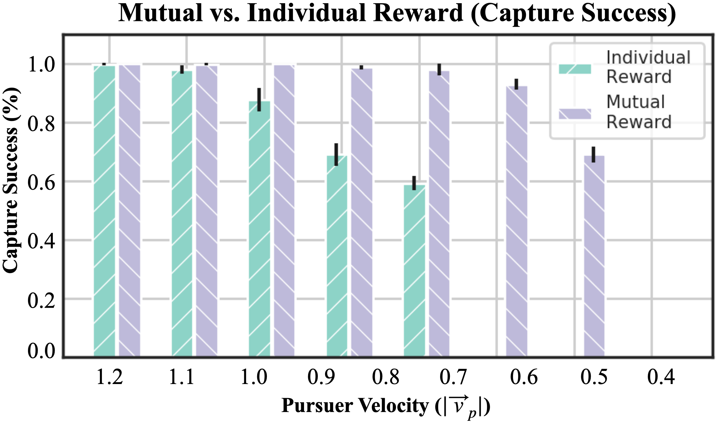
Figure 2: Performance of policies trained with individual vs. mutual reward. As pursuer velocity decreases, the pursuit-evasion task requires more sophisticated coordination.

5.2 Fair outcomes with Fair-E

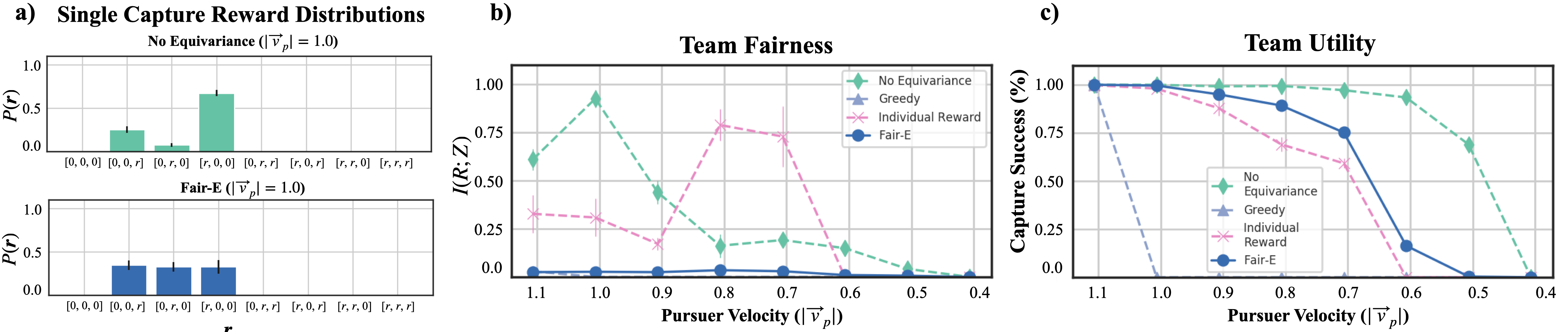
Figure 3: Quantitative comparison of performance for equivariant (i.e. Fair-E) vs. non-equivariant policies. a) Distribution of reward vectors for both strategies at the pursuer velocity $\lvert\vec{v}_{p}\rvert=1.0$. Non-equivariant policies (top), which learn strategies that push captures towards one agent, yield highly uneven reward distributions. Fair-E policies (bottom) learn to spread captures amongst teammates equally, resulting in even reward distributions. b) Team fairness scores for both strategies (lower better). Fair-E policies yield fairer outcomes than non-equivariant policies across all pursuer velocity (i.e. agent skill) levels. Note that the curve for the Greedy strategy, which is fair despite its low utility, is tucked behind the Fair-E curve. c) Team utility (i.e. capture success) achieved by both strategies (higher better). As pursuer velocity decreases, non-equivariant policies outperform Fair-E by a wide margin, indicating that a fairness-utility trade-off exists.

Though mutual reward incentivizes efficient team coordination, it does not stipulate how agents should coordinate. To study the nature of the resulting strategy, we examine the distribution of reward vectors obtained by the pursuers over 100 test-time trajectories (averaged over five random seeds each). As shown in Figure 3a (top), in which we plot reward vector assignments for captures involving only one pursuer, the pursuer team discovers an unfair strategy—the majority of captures are accounted for by a single agent.

The emergence of an unfair strategy reflects the difficulty of the pursuit-evasion setting. As $\lvert\vec{v}_{p}\rvert$ decreases, the whole pursuer team has to learn to work together to capture the evader, which is a challenging coordination task. The pursuers learn to do this effectively by assigning roles — e.g. in the $n{=}3$ case, two pursuers take supporting roles, shepherding the evader towards the third agent, who is designated the “capturer”. We note that the decision of which agent becomes the capturer is an emergent phenomenon of the system. As $\lvert\vec{v}_{p}\rvert$ decreases further, such role assignment is not only helpful but necessary for success. Altogether, the results suggest that unconstrained mutual reward maximization prioritizes utility over fairness.

Our proposed solution, Fair-E, directly combats these fairness issues. Figure 3a (bottom) shows the distribution of reward vectors obtained by agents trained with Fair-E. Due to equivariance, Fair-E yields much more evenly distributed rewards. To further quantify these gains, we compare team fairness for both strategies over a variety of skill levels (i.e. $\lvert\vec{v}_{p}\rvert$ values). The results, shown in Figure 3b, confirm that Fair-E achieves much lower $I(R;Z)$ and, therefore, higher team-fairness. Note that, when $\lvert\vec{v}_{p}\rvert<0.9$, $I(R;Z)$ is low for non-equivariant pursuers as well. This is an artifact of team fairness—as $\lvert\vec{v}_{p}\rvert$ decreases, capture success inevitably decreases as well, which is technically a fairer, albeit less desirable, outcome (all agents share equitably in failure). Nevertheless, Figure 3b serves as empirical evidence to backup our theoretical result from Section 4.2 that Fair-E meets the demands of team fairness.

Despite achieving fairer outcomes, Fair-E is subject to drops in utility as $\lvert\vec{v}_{p}\rvert$ decreases (see Figure 3c). The utility curve for Fair-E drops precipitously for agent skill $\lvert\vec{v}_{p}\rvert<0.9$; much faster than the drop-off for pursuers with no equivariance. This is because Fair-E directly prevents role assignment. By hard-constraining each agent’s policy, Fair-E enforces $\pi_{i}(s_{t}){=}\pi_{j}(s_{t})$, whereas role assignment requires $\pi_{i}(s_{t}){\neq}\pi_{j}(s_{t})$ for $i{\neq}j$. We emphasize role assignment as key to this result, as parameter-sharing has been shown to be helpful in problem domains that do not require explicit role assignment (Baker et al. 2019). In the context of fairness, however, these results indicate that Fair-E will always elect to give up utility to preserve fairness.

For completeness, we also show results for the policies learned with individual reward (from Figure 2) and a hand-crafted greedy control strategy in which each pursuer runs directly towards the evader. Note that greedy policies are equivariant—by definition, agents will select similar actions in similar states—but demonstrate no coordination. For this reason, greedy policies have high fairness, but very low utility. Utility follows the same pattern for individual reward policies. Interestingly though, individual reward policies become less fair between $\lvert\vec{v}_{p}\rvert=0.9$ and $\lvert\vec{v}_{p}\rvert=0.6$, before tapering off as performance decreases. We defer further discussion of this finding, as well as details regarding the computation of the team fairness score, $I(R;Z)$, and the hand-crafted greedy control baseline to Appendix C.

5.3 Modulating fairness with Fair-ER

Unlike Fair-E, Fair-ER allows policies to balance fairness and utility dynamically. Intuitively, this is because Fair-ER incentivizes policy equivariance through the regularization objective from Equation (9), while still allowing agents to update their own individual policy parameters (unlike Fair-E). Therefore, the value of the fairness control weight $\lambda$ will dictate how much each agent values fairness vs. utility.

To study the effectiveness of this method, we trained Fair-ER agents in increasingly difficult environments (by decreasing pursuer velocity $\lvert\vec{v}_{p}\rvert$) while modulating the fairness control parameter $\lambda$. The effect of $\lambda$ on policy training is shown in Figure 4. The results show that, for $\lambda{\leq}0.5$, Fair-ER is successful in bridging the performance gap between non-equivariant policies ($\lambda{=}0.0)$ and Fair-E (black line). Importantly, we show that it is also possible to over-constrain the system so that it actually performs worse than Fair-E (e.g. $\lambda{=}1.0$). This indicates that, though Fair-ER can mitigate the drops in performance described above, the regularization parameter $\lambda$ must be tuned appropriately.

We also performed the same test-time analysis as described for Fair-E in the previous subsection. Figure 5 shows the effect of $\lambda$ on both fairness ($I(R;Z)$) and utility (capture success). For each skill level, increasing $\lambda$ allows Fair-ER to fine-tune the balance between fair and unfair policies, achieving the highest utility possible under its given constraints. We find that, with high values of $\lambda$ (e.g. $\lambda=0.9$), Fair-ER prioritizes fairness over utility and performs in-line with (or worse than) Fair-E—achieving fair outcomes, even at the expense of utility. When $\lambda$ is in the range $\lambda=0.5$ to $\lambda=0.1$, Fair-ER withstands a drop in utility until $\lvert\vec{v}_{p}\rvert=0.7$ by giving up small amounts of fairness. Therefore, we find evidence that learning multi-agent coordination strategies with Fair-ER simultaneously maintains higher utility than Fair-E while achieving higher fairness than non-equivariant learning. Overall, tuning the fairness weight $\lambda$ allows us to directly control the strength of the fairness constraints imposed on the system, enabling Fair-ER to modulate fairness to the needs of the task.

5.4 Fairness-utility trade-off

As we saw in Figure 3, the hard constraints that Fair-E places on each agent’s policy creates an inherent commitment to achieving fair outcomes at the expense of utility (or reward). In this section, we examine the extent to which the fairness-utility trade-off exists for Fair-ER across all agent skill levels. For each agent skill level (i.e. $\lvert\vec{v}_{p}\rvert$ value), we computed both the fairness (through team fairness $I(R;Z)$) and utility (through capture success) scores achieved by multi-agent coordination strategies learned for $\lambda$ values in the range $\lambda\in\{0.0,1.0\}$ over 100 test-time trajectories (averaged over five random seeds each). The results of this experiment are shown in Figure 5.

Unlike many prior studies in both traditional multi-agent fairness settings (Okun 1975; Le Grand 1990; Bertsimas, Farias, and Trichakis 2012; Joe-Wong et al. 2013; Bertsimas, Farias, and Trichakis 2011) and prediction-based settings (Corbett-Davies et al. 2017; Zhao and Gordon 2019), we find that it is not always the case that fairness must be traded for utility. With Fair-ER, fairness comes for little to no cost in utility until $\lvert\vec{v}_{p}\rvert=0.8$. This means that, when each agent operates at a high skill level, requiring each agent in the multi-agent team to shift towards an equivariant policy (which yields fair results) does not cause coordination of the larger multi-agent team to break down. When $\lvert\vec{v}_{p}\rvert<0.8$, however, utility drops quickly for larger values of $\lambda$. This indicates that, when agent skill decreases (or the task becomes more complex relative the agents’ current skill level), unfair strategies such as role assignment are the only effective way to maintain high levels of utility. Overall, these results serve as empirical evidence that, in the context of cooperative multi-agent tasks, fairness is inexpensive, so long as the task is easy enough (i.e. agent skill is high enough). As task difficulty increases, fairness comes at an increasingly steep cost. To the best of our knowledge, such a characterization of the fairness-utility trade-off for multi-agent settings has not been illustrated in the fairness literature.

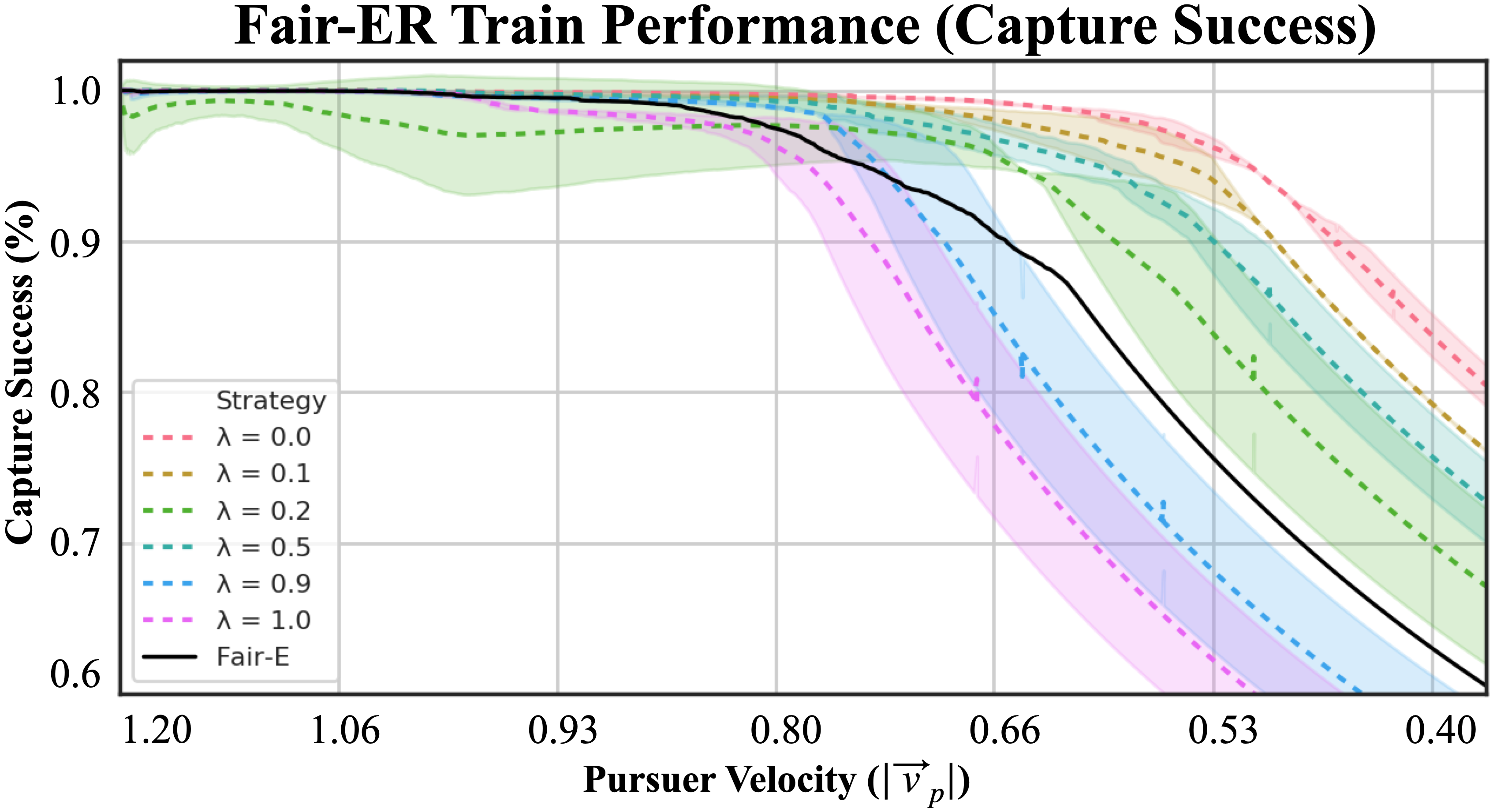
Figure 4: Effect of the equivariance control parameter $\lambda$ on policy learning with Fair-ER. Increasing $\lambda$ yields fairer policies, but causes performance to decay more quickly in difficult environments (lower agent skill). The black line represents Fair-E’s performance for comparison.

6 Conclusion

Multi-agent learning holds promise for helping AI researchers, economic theorists, and policymakers alike better evaluate real-world problems involving social structures, taxation, policy, and economic systems broadly. This work has focused on one such problem; namely, fairness in cooperative multi-agent settings. In particular, we have demonstrated that fairness issues arise naturally in cooperative, single-objective multi-agent learning problems. We have shown that our proposed method, equivariant policy optimization (Fair-E), mitigates such issues. We have also shown that soft constraints (Fair-ER) lower the cost of fairness and allow the fairness-utility trade-off to be balanced dynamically. Moreover, we have presented novel results regarding the fairness-utility trade-off for cooperative multi-agent settings; identifying a connection between agent skill and fairness. In particular, we showed that fairness comes for free when agents are highly-skilled, but becomes increasingly expensive for lesser-skilled agents.

This work represents a first step towards understanding the core factors underlying fairness and multi-agent learning in environments where team dynamics and coordination are important for task success. There are a number of exciting avenues of future work that build upon these initial ideas. First, ongoing work is investigating cooperative multi-agent fairness in more complex domains (e.g. video games, simulated economic societies). Moreover, there is room to explore indirect or backdoor causal paths between sensitive and target variables in the context of multi-agent teams, which warrant connecting additional interpretations of fairness (e.g. causal fairness) to cooperative multi-agent settings.

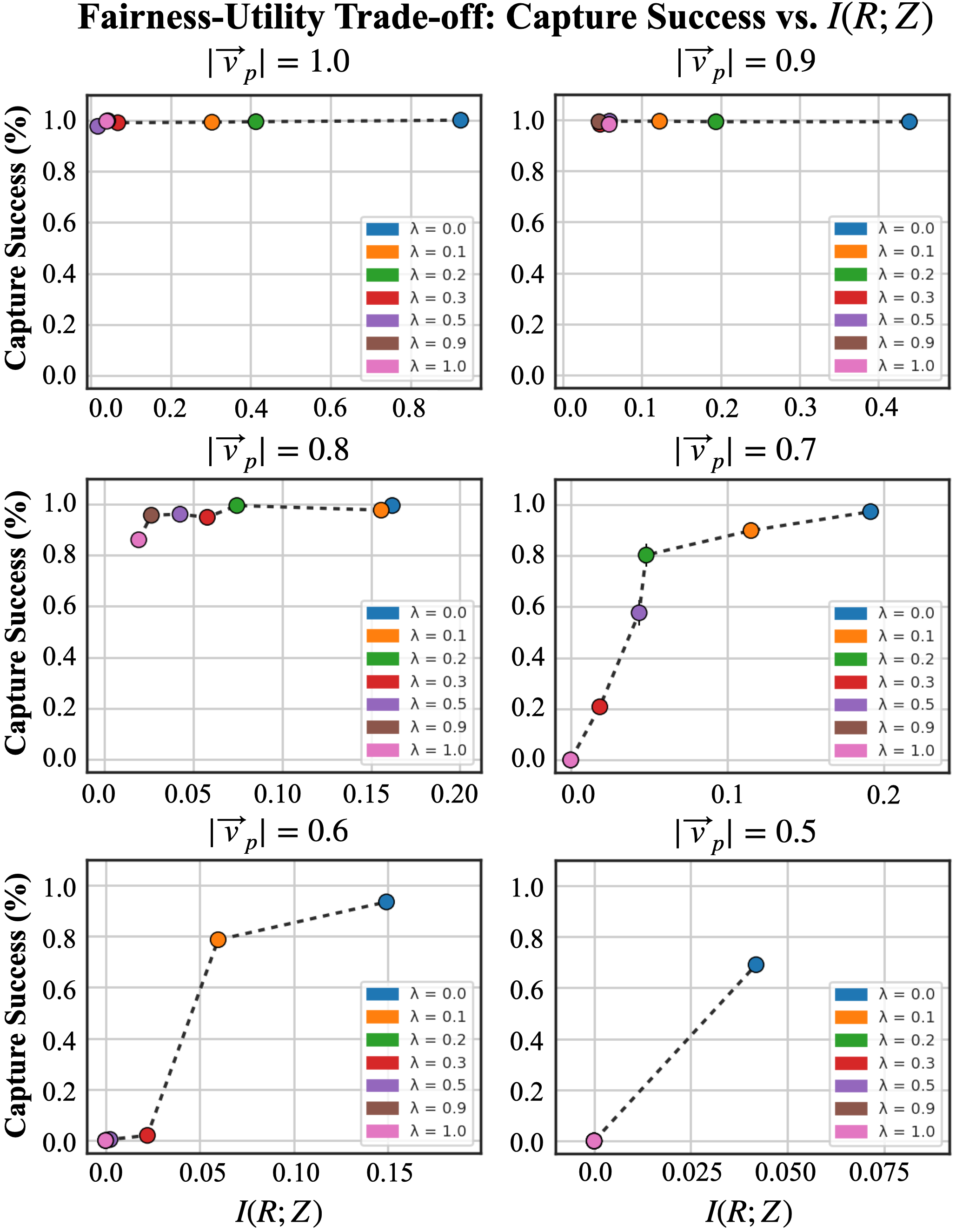
Figure 5: Fairness vs. utility comparisons for Fair-ER trained with various values of equivariance regularization $\lambda$ and environment difficulties. Note that $\lambda=0.0$ is equivalent to no equivariance.

Appendix A Deterministic fairness through equivariance

We review the proofs from Section 4.2 in the context of deterministic policies. We assume that agents are homogeneous in their non-sensitive variables. For $n$ agents, each with an individual policy $\mu_{\phi_{i}}$, let $\boldsymbol{\mu}=\{\mu_{\phi_{1}},...,\mu_{\phi_{n}}\}$ be the joint policy representing the team. Recall that, in the symmetric case, $\phi_{1}=\phi_{2}=...=\phi_{n}$ and $\omega_{1}=\omega_{2}=...=\omega_{n}$.

Theorem 1.

If individual policies $\mu_{\phi_{i}}$ are symmetric, then the joint policy $\boldsymbol{\mu}=\{\mu_{\phi_{1}},...,\mu_{\phi_{n}}\}$ is an equivariant map.

Proof.

Let $\sigma$ be a permutation operator that, when applied to a vector (such as a state $s_{t}$ or joint action $\boldsymbol{a}_{t}$), produces the permuted vector ($\sigma\cdot s_{t}{=}s^{\sigma}_{t}$ or $\sigma\cdot\boldsymbol{a}_{t}{=}\boldsymbol{a}^{\sigma}_{t}$, respectively). Under parameter symmetry (i.e. $\phi_{1}$=$\phi_{2}{=}{\cdots}{=}\phi_{n}$), we have:

$$\boldsymbol{\mu}(\sigma\cdot s)=\boldsymbol{\mu}(s^{\sigma})\\ =\boldsymbol{a}^{\sigma}\\ =\sigma\cdot\boldsymbol{a}\\ =\sigma\cdot\boldsymbol{\mu}(s)$$

where the commutative relationship $\boldsymbol{\mu}(\sigma\cdot s)=\sigma\cdot\boldsymbol{\mu}(s)$ implies that $\boldsymbol{\mu}$ is an equivariant map. ∎

Theorem 2.

Let $p^{\boldsymbol{\mu}}(s\rightarrow s^{\prime},k)$ be the probability of transitioning from $s$ to $s^{\prime}$ in $k$ steps. Given that the joint policy $\boldsymbol{\mu}$ is an equivariant map, it follows that $p^{\boldsymbol{\mu}}(s_{1}\rightarrow s_{T},T)=p^{\boldsymbol{\mu}}(s_{1}^{\sigma}\rightarrow s_{T}^{\sigma},T)$.

Proof.

It follows from agent homogeneity that permuting a state $\sigma\cdot s_{t}$, which in turn permutes action selection $\sigma\cdot\boldsymbol{a}_{t}$ (from Theorem 1), also permutes the environment’s transition probabilities:

$$P(s_{t+1}|s_{t},a_{t})=P(s_{t+1}^{\sigma}|s_{t}^{\sigma},\boldsymbol{a}_{t}^{\sigma})$$

This is because, from the environment’s perspective, a state-action pair is indistinguishable from the state-action pair generated by the same agents after swapping their positions and selected actions. Assuming that the full distribution of start-states $P_{\emptyset}$ is uniform, we also have $P_{\emptyset}(s_{1})=P_{\emptyset}(s_{1}^{\sigma})$. Recall the probability of a trajectory from Equation (1). Given the equivariant function $\boldsymbol{\mu}$ and the two equalities above, it follows that:

$$P_{\emptyset}(s_{1})\prod_{t=1}^{T} P(s_{t+1}|s_{t},\boldsymbol{a}_{t})|_{\boldsymbol{a}_{t}=\boldsymbol{\mu}(s_{t})}$$

$$=P_{\emptyset}(s_{1}^{\sigma})\prod_{t=1}^{T}P(s_{t+1}^{\sigma}|s_{t}^{\sigma},\boldsymbol{a}_{t}^{\sigma})|_{\boldsymbol{a}_{t}^{\sigma}=\boldsymbol{\mu}(s_{t}^{\sigma})}$$

Note that the following properties hold for $p^{\boldsymbol{\mu}}(s\rightarrow s^{\prime},k)$:

• $p^{\boldsymbol{\mu}}(s\rightarrow s,0)=1$

• $p^{\boldsymbol{\mu}}(s\rightarrow s^{\prime},1)=p(s_{t+1}=s^{\prime}|s_{t}=s,a_{t})|a_{t}=\mu(s_{t})$,

• $p^{\boldsymbol{\mu}}(s\rightarrow x,T)=\int_{s^{\prime}}p^{\mu}(s\rightarrow s^{\prime},T-1)p^{\mu}(s^{\prime}\rightarrow x,1)$

We can therefore represent the probability of a trajectory as a single transition from initial state $s_{1}$ to terminal state $s_{T}$ by marginalizing out the intermediate states and show that:

$$p^{\mu}(s_{1}\rightarrow s_{T},T)$$

$$=\int_{s_{T-1}}p^{\mu}(s_{1}\rightarrow s_{T-1},T-1)p^{\mu}(s_{T-1}\rightarrow s_{T},1)$$

$$\begin{multlined}=\int_{s_{T-2}}p^{\mu}(s_{1}\rightarrow s_{T-2},T-2)\big{[}p^{\mu}(s_{T-2}\rightarrow s_{T-1},1)\\ p^{\mu}(s_{T-1}\rightarrow s_{T},1)\big{]}\end{multlined}=\int_{s_{T-2}}p^{\mu}(s_{1}\rightarrow s_{T-2},T-2)\big{[}p^{\mu}(s_{T-2}\rightarrow s_{T-1},1)\\ p^{\mu}(s_{T-1}\rightarrow s_{T},1)\big{]}$$

$$=\cdots$$

$$=\int_{s_{1}}\cdots\int_{s_{T-1}}P_{\emptyset}(s_{1})\prod_{t=1}^{T}P(s_{t+1}|s_{t},a_{t})|_{a_{t}=\mu(s_{t})}$$

$$=\int_{s_{1}^{\sigma}}\cdots\int_{s_{T-1}^{\sigma}}P_{\emptyset}(s_{1}^{\sigma})\prod_{t=1}^{T}P(s_{t+1}^{\sigma}|s_{t}^{\sigma},a_{t}^{\sigma})|_{a_{t}^{\sigma}=\mu(s_{t}^{\sigma})}$$

$$=\cdots$$

$$=p^{\mu}(s_{1}^{\sigma}\rightarrow s_{T}^{\sigma},T)$$

Thus, the probability of reaching terminal state $s_{T}$ from initial state $s_{1}$ is equivalent to the probability of reaching $s_{T}^{\sigma}$ from $s_{1}^{\sigma}$. ∎

Theorem 3.

Equivariant deterministic policies are exactly fair.

Proof.

Exact same as Theorem 3. ∎

Appendix B Derivations

B.1 Gradient of fairness objective

We present a derivation of the equivariant objective gradient from Equation (11):

$$\frac{\partial J_{\textrm{eqv}}}{\partial\phi_{i}} \approx\frac{\partial}{\partial\phi_{i}}\frac{1}{M}\sum_{i}^{M}\frac{1}{N-1}\sum_{j\neq i}^{N-1}1-\cos(\mu_{\phi_{i}}(s)-\mu_{\phi_{j}}(s))$$

$$\begin{multlined}=\frac{1}{M}\sum_{i}^{M}\frac{1}{N-1}\sum_{j\neq i}^{N-1}-(-\sin(\mu_{\phi_{i}}(s)\\ \qquad\qquad-\mu_{\phi_{j}}(s)))\frac{\partial}{\partial\phi_{i}}(\mu_{\phi_{i}}(s)-\mu_{\phi_{j}}(s))\end{multlined}=\frac{1}{M}\sum_{i}^{M}\frac{1}{N-1}\sum_{j\neq i}^{N-1}-(-\sin(\mu_{\phi_{i}}(s)\\ \qquad\qquad-\mu_{\phi_{j}}(s)))\frac{\partial}{\partial\phi_{i}}(\mu_{\phi_{i}}(s)-\mu_{\phi_{j}}(s))$$

$$\begin{multlined}=\frac{1}{M}\sum_{i}^{M}\frac{1}{N-1}\sum_{j\neq i}^{N-1}\sin(\mu_{\phi_{i}}(s)\\ \qquad\qquad-\mu_{\phi_{j}}(s))\bigg{(}\frac{\partial}{\partial\phi_{i}}\mu_{\phi_{i}}(s)-\frac{\partial}{\partial\phi_{i}}\mu_{\phi_{j}}(s)\bigg{)}\end{multlined}=\frac{1}{M}\sum_{i}^{M}\frac{1}{N-1}\sum_{j\neq i}^{N-1}\sin(\mu_{\phi_{i}}(s)\\ \qquad\qquad-\mu_{\phi_{j}}(s))\bigg{(}\frac{\partial}{\partial\phi_{i}}\mu_{\phi_{i}}(s)-\frac{\partial}{\partial\phi_{i}}\mu_{\phi_{j}}(s)\bigg{)}$$

$$\begin{multlined}=\frac{1}{M}\sum_{i}^{M}\frac{1}{N-1}\sum_{j\neq i}^{N-1}\sin(\mu_{\phi_{i}}(s)\\ \qquad\qquad-\mu_{\phi_{j}}(s))\nabla_{\phi_{i}}\mu_{\phi_{i}}(s)\end{multlined}=\frac{1}{M}\sum_{i}^{M}\frac{1}{N-1}\sum_{j\neq i}^{N-1}\sin(\mu_{\phi_{i}}(s)\\ \qquad\qquad-\mu_{\phi_{j}}(s))\nabla_{\phi_{i}}\mu_{\phi_{i}}(s)$$

B.2 Why not mean squared error?

We could just have as easily defined $J_{\textrm{eqv}}$ as the mean-squared error (MSE) between $a_{i}$ and $a_{j}$, with the objective:

$$J_{\textrm{sym}}(\phi_{1},...,\phi_{i},...,\phi_{n})=\mathbb{E}_{s}[\mathbb{E}_{j\neq i}[(\mu_{\phi_{i}}(s)-\mu_{\phi_{j}}(s))^{2}]]$$

and corresponding gradient:

$$\nabla_{\phi_{i}}J_{\textrm{sym}}(\phi)\approx\frac{1}{M}\sum_{i}\frac{1}{N-1}\sum_{j\neq i}(\mu_{\phi_{i}}(s)\\ -\mu_{\phi_{j}}(s))\nabla_{\phi_{i}}\mu_{\phi_{i}}(s)|_{s=s_{i}}$$

However, recall that each $a$ is a heading angle sampled from $A$, which is a circular variable in the range $[0,2\pi]$ or $[-\pi,\pi]$. Any difference of actions, as in MSE loss, must account for this by applying a modulo operation on top of the difference. Our objective represents angular distance as a single Fourier mode, which yields a convex optimization surface without discontinuity issues on the range of possible headings.

Appendix C Experimental details

Computing team fairness

We illustrate how team fairness scores $I(R;Z)$ are computed. Recall that each agent’s sensitive attribute $z_{i}$ is an identity variable that uniquely identifies it from the group (see Section 5.1). Also note that the vectorial reward vector $\boldsymbol{r}$ serves as a proxy for agent identity—e.g. $\boldsymbol{r}{=}[0,0,1]$ indicates that pursuer $p_{3}$ captured the evader. We can therefore compute team fairness as the mutual information obtained by the difference of entropies $h(R)-h(R_{\textrm{uniform}})$, where $R$ is a distribution over team rewards $\boldsymbol{r}$ and $R_{\textrm{uniform}}$ is a uniform reward distribution (i.e. captures are spread evenly across all pursuers). Computed this way, $I(R;Z)$ represents the extent to which knowing the outcome of the pursuit-evasion task reveals the agents identity, and vice versa. It therefore measures how fairly outcomes are distributed across cooperative teammates.

Greedy control baseline

Let $q_{i}$ be the position of an agent $i$ and $U_{\textrm{att}}(q_{i})$ be a quadratic function of distance between $q_{i}$ and a target $q_{\textrm{goal}}$:

$$U_{\textrm{att}}(q_{i},q_{\textrm{goal}})=\frac{1}{2}k_{\textrm{att}}\,d(q_{i},q_{\textrm{goal}})^{2}$$ (12)

where $k_{\textrm{att}}$ is an attraction coefficient and $d(,)$ is a measure of distance. Taking the negative gradient $F(q_{i})=-\nabla U(q_{i})$ yields the following control law for agent $i$’s motion:

$$F_{\textrm{att}}=-\nabla U_{\textrm{att}}(q_{i},q_{\textrm{goal}})=-k_{\textrm{att}}(q_{i}-q_{\textrm{goal}})$$ (13)

In this work, the environment’s action-space is defined in terms of agent headings, so only the direction of this force impacts the agents. Setting $q_{\textrm{goal}}$ to be the position of the evader and following Equation (12) at each time-step results in a greedy policy that runs directly towards the evader.

Fairness for individual reward policies

In Figure 3b, we find that policies learned with individual reward exhibit a temporary spike in $I(R;Z)$ from $\lvert\vec{v}_{p}\rvert=0.9$ to $\lvert\vec{v}_{p}\rvert=0.6$, indicating that their reward distributions $R$ are less fair. This occurs because, as $\lvert\vec{v}_{p}\rvert$ decreases, policies learned with individual reward fall into a degenerate state where only one pursuer experiences positive reward from capturing the evader. The other pursuers, never experiencing positive reward, slowly diverge from their previous greedy strategies and become incapable of capturing the evader. Their best strategy becomes hoping that the “capturer” pursuer captures the evader, which results in a highly skewed capture distribution. Eventually this strategy fails when $\lvert\vec{v}_{p}\rvert$ drops low enough that all pursuers fail to capture the evader, which causes $I(R;Z)$ to fall again.

Policy learning hyperparameters

All actors $\mu_{\phi}$ are trained with two hidden layers of size 128. Critics $Q_{\omega}$ are trained with three hidden layers of size 128. We use a learning rate of $1\textrm{e}^{-4}$ and $1\textrm{e}^{-3}$ for the actor and critic, respectively, and a gradient clip of 0.5 on both. Target networks are updated with Polyak averaging with $\tau=0.001$. We maintain a buffer $\mathcal{D}$ of length $500000$ and sample batches of size $512$. Finally, we use a discount factor $\gamma=0.99$. All values are the results of standard hyperparamter sweeps.

Experiments

As described in Section 5.1, each pursuit-evasion experiment includes $n=3$ pursuer agents and a single evader. The pursuers each train their own policy for a total of 125,000 episodes, during which their velocity is decreased from $\lvert\vec{v}_{p}\rvert=1.2$ to $\lvert\vec{v}_{p}\rvert=0.4$. The evader speed is fixed at $\lvert\vec{v}_{e}\rvert=1.0$. After training, we test the resulting policies at discrete velocity intervals (e.g. $\lvert\vec{v}_{p}\rvert=1.2$, $\lvert\vec{v}_{p}\rvert=1.1$, etc), where a decrease in pursuer velocity represents a greater “difficulty level” for the pursuers. Test-time performance, such as is shown in Figures 2b, 3c, 3d, and 5 is averaged across 100 independent trajectories from five different random seeds each. All experiments leveraged an Nvidia GeForce GTX 1070 GPU with 8GB of memory.

Appendix D Additional information

Assets

The pursuit-evasion environment used in this work is an extension of the environment introduced by Lowe et al. (2017). The original environment is open-sourced on Github under the MIT license. We cited the authors accordingly in the main text. Since we only change the reward function, we do not include the pursuit-evasion environment as a new asset in the supplementary material. Instead, we point to the original repo. None of the assets used in this work contain personally identifiable information or offensive content.

Limitations

In our Fair-ER learning strategy, the fairness control parameter $\lambda$ allows the strength of equivariance regularization to be tuned to achieve the desired fairness-utility trade-off for the task at hand. Despite these benefits, tuning $\lambda$ is currently a manual process. An ideal solution, which is the subject of future work, would automatically find the appropriate $\lambda$ value for the desired fairness-utility trade-off. We highlight, however, that many regularization techniques in machine learning (most notably, $L_{1}$ and $L_{2}$ regularization) require manual tuning as well.

Moreover, our method does not directly address non-stationarity in multi-agent RL. Non-stationarity can cause high variance policy gradients and learning instability. This did not significantly impact training in our case, but possible solutions, such as centralized training (Foerster et al. 2016; Lowe et al. 2017) will be considered in future work. Though we primarily evaluate our method in the context of pursuit-evasion games, we highlight that both Fair-E and Fair-ER are task-agnostic—they can be applied to any multi-agent environment.

References

- Baker et al. (2019) Baker, B.; Kanitscheider, I.; Markov, T.; Wu, Y.; Powell, G.; McGrew, B.; and Mordatch, I. 2019. Emergent tool use from multi-agent autocurricula. arXiv preprint arXiv:1909.07528.
- Barocas, Hardt, and Narayanan (2019) Barocas, S.; Hardt, M.; and Narayanan, A. 2019. Fairness and Machine Learning. fairmlbook.org. http://www.fairmlbook.org.
- Bertsimas, Farias, and Trichakis (2011) Bertsimas, D.; Farias, V. F.; and Trichakis, N. 2011. The price of fairness. Operations research, 59(1): 17–31.
- Bertsimas, Farias, and Trichakis (2012) Bertsimas, D.; Farias, V. F.; and Trichakis, N. 2012. On the efficiency-fairness trade-off. Management Science, 58(12): 2234–2250.
- Calders, Kamiran, and Pechenizkiy (2009) Calders, T.; Kamiran, F.; and Pechenizkiy, M. 2009. Building classifiers with independency constraints. In 2009 IEEE International Conference on Data Mining Workshops, 13–18. IEEE.
- Chouldechova and Roth (2018) Chouldechova, A.; and Roth, A. 2018. The frontiers of fairness in machine learning. arXiv preprint arXiv:1810.08810.
- Corbett-Davies et al. (2017) Corbett-Davies, S.; Pierson, E.; Feller, A.; Goel, S.; and Huq, A. 2017. Algorithmic decision making and the cost of fairness. In Proceedings of the 23rd acm sigkdd international conference on knowledge discovery and data mining, 797–806.
- De Jong et al. (2005) De Jong, S.; Tuyls, K.; Verbeeck, K.; and Roos, N. 2005. Priority awareness: towards a computational model of human fairness for multi-agent systems. In Adaptive Agents and Multi-Agent Systems III. Adaptation and Multi-Agent Learning, 117–128. Springer.
- De Jong et al. (2007) De Jong, S.; Tuyls, K.; Verbeeck, K.; and Roos, N. 2007. Considerations for fairness in multi-agent systems.
- Dorans and Cook (2016) Dorans, N. J.; and Cook, L. L. 2016. Fairness in educational assessment and measurement. Routledge.
- Dwork et al. (2012) Dwork, C.; Hardt, M.; Pitassi, T.; Reingold, O.; and Zemel, R. 2012. Fairness through awareness. In Proceedings of the 3rd innovations in theoretical computer science conference, 214–226.
- Elzayn et al. (2019) Elzayn, H.; Jabbari, S.; Jung, C.; Kearns, M.; Neel, S.; Roth, A.; and Schutzman, Z. 2019. Fair algorithms for learning in allocation problems. In Proceedings of the Conference on Fairness, Accountability, and Transparency, 170–179.
- Feldman et al. (2015) Feldman, M.; Friedler, S. A.; Moeller, J.; Scheidegger, C.; and Venkatasubramanian, S. 2015. Certifying and removing disparate impact. In proceedings of the 21th ACM SIGKDD international conference on knowledge discovery and data mining, 259–268.
- Foerster et al. (2016) Foerster, J. N.; Assael, Y. M.; De Freitas, N.; and Whiteson, S. 2016. Learning to communicate with deep multi-agent reinforcement learning. arXiv preprint arXiv:1605.06676.
- Fuster et al. (2020) Fuster, A.; Goldsmith-Pinkham, P.; Ramadorai, T.; and Walther, A. 2020. Predictably unequal? The effects of machine learning on credit markets. The Effects of Machine Learning on Credit Markets.
- Grupen, Lee, and Selman (2020) Grupen, N. A.; Lee, D. D.; and Selman, B. 2020. Low-Bandwidth Communication Emerges Naturally in Multi-Agent Learning Systems. arXiv preprint arXiv:2011.14890.
- Hao and Leung (2016) Hao, J.; and Leung, H.-f. 2016. Fairness in Cooperative Multiagent Systems. In Interactions in Multiagent Systems: Fairness, Social Optimality and Individual Rationality, 27–70. Springer.
- Hardt, Price, and Srebro (2016) Hardt, M.; Price, E.; and Srebro, N. 2016. Equality of opportunity in supervised learning. arXiv preprint arXiv:1610.02413.
- Hughes et al. (2018) Hughes, E.; Leibo, J. Z.; Phillips, M. G.; Tuyls, K.; Duéñez-Guzmán, E. A.; Castañeda, A. G.; Dunning, I.; Zhu, T.; McKee, K. R.; Koster, R.; et al. 2018. Inequity aversion improves cooperation in intertemporal social dilemmas. arXiv preprint arXiv:1803.08884.
- Isaacs (1999) Isaacs, R. 1999. Differential games: a mathematical theory with applications to warfare and pursuit, control and optimization. Courier Corporation.
- Jabbari et al. (2017) Jabbari, S.; Joseph, M.; Kearns, M.; Morgenstern, J.; and Roth, A. 2017. Fairness in reinforcement learning. In International Conference on Machine Learning, 1617–1626. PMLR.
- Jiang and Lu (2019) Jiang, J.; and Lu, Z. 2019. Learning fairness in multi-agent systems. arXiv preprint arXiv:1910.14472.
- Joe-Wong et al. (2013) Joe-Wong, C.; Sen, S.; Lan, T.; and Chiang, M. 2013. Multiresource allocation: Fairness–efficiency tradeoffs in a unifying framework. IEEE/ACM Transactions on Networking, 21(6): 1785–1798.
- Johndrow, Lum et al. (2019) Johndrow, J. E.; Lum, K.; et al. 2019. An algorithm for removing sensitive information: application to race-independent recidivism prediction. The Annals of Applied Statistics, 13(1): 189–220.
- Kamiran and Calders (2009) Kamiran, F.; and Calders, T. 2009. Classifying without discriminating. In 2009 2nd International Conference on Computer, Control and Communication, 1–6. IEEE.
- Kleinberg, Mullainathan, and Raghavan (2016) Kleinberg, J.; Mullainathan, S.; and Raghavan, M. 2016. Inherent trade-offs in the fair determination of risk scores. arXiv preprint arXiv:1609.05807.
- Lahoti, Gummadi, and Weikum (2019) Lahoti, P.; Gummadi, K. P.; and Weikum, G. 2019. Operationalizing individual fairness with pairwise fair representations. arXiv preprint arXiv:1907.01439.
- Le Grand (1990) Le Grand, J. 1990. Equity versus efficiency: the elusive trade-off. Ethics, 100(3): 554–568.
- Leibo et al. (2017) Leibo, J. Z.; Zambaldi, V.; Lanctot, M.; Marecki, J.; and Graepel, T. 2017. Multi-agent reinforcement learning in sequential social dilemmas. arXiv preprint arXiv:1702.03037.
- Li et al. (2021) Li, J.; Kuang, K.; Wang, B.; Liu, F.; Chen, L.; Wu, F.; and Xiao, J. 2021. Shapley Counterfactual Credits for Multi-Agent Reinforcement Learning. arXiv preprint arXiv:2106.00285.
- Lillicrap et al. (2015) Lillicrap, T. P.; Hunt, J. J.; Pritzel, A.; Heess, N.; Erez, T.; Tassa, Y.; Silver, D.; and Wierstra, D. 2015. Continuous control with deep reinforcement learning. arXiv preprint arXiv:1509.02971.
- Littman (1994) Littman, M. L. 1994. Markov games as a framework for multi-agent reinforcement learning. In Machine learning proceedings 1994, 157–163. Elsevier.
- Liu et al. (2018) Liu, L. T.; Dean, S.; Rolf, E.; Simchowitz, M.; and Hardt, M. 2018. Delayed impact of fair machine learning. In International Conference on Machine Learning, 3150–3158. PMLR.
- Lowe et al. (2017) Lowe, R.; Wu, Y.; Tamar, A.; Harb, J.; Abbeel, P.; and Mordatch, I. 2017. Multi-agent actor-critic for mixed cooperative-competitive environments. arXiv preprint arXiv:1706.02275.
- Menon and Williamson (2018) Menon, A. K.; and Williamson, R. C. 2018. The cost of fairness in binary classification. In Conference on Fairness, Accountability and Transparency, 107–118. PMLR.
- Mitchell et al. (2018) Mitchell, S.; Potash, E.; Barocas, S.; D’Amour, A.; and Lum, K. 2018. Prediction-based decisions and fairness: A catalogue of choices, assumptions, and definitions. arXiv preprint arXiv:1811.07867.
- Mordatch and Abbeel (2018) Mordatch, I.; and Abbeel, P. 2018. Emergence of grounded compositional language in multi-agent populations. In Proceedings of the AAAI Conference on Artificial Intelligence, volume 32.
- Okun (1975) Okun, A. M. 1975. Equality and efficiency: The big tradeoff. Brookings Institution Press.
- Pannekoek and Spigler (2021) Pannekoek, M.; and Spigler, G. 2021. Investigating Trade-offs in Utility, Fairness and Differential Privacy in Neural Networks. arXiv preprint arXiv:2102.05975.
- Peysakhovich and Lerer (2017) Peysakhovich, A.; and Lerer, A. 2017. Prosocial learning agents solve generalized stag hunts better than selfish ones. arXiv preprint arXiv:1709.02865.
- Potash et al. (2015) Potash, E.; Brew, J.; Loewi, A.; Majumdar, S.; Reece, A.; Walsh, J.; Rozier, E.; Jorgenson, E.; Mansour, R.; and Ghani, R. 2015. Predictive modeling for public health: Preventing childhood lead poisoning. In Proceedings of the 21th ACM SIGKDD International Conference on Knowledge Discovery and Data Mining, 2039–2047.
- Rapoport (1974) Rapoport, A. 1974. Prisoner’s dilemma—recollections and observations. In Game Theory as a Theory of a Conflict Resolution, 17–34. Springer.
- Ravanbakhsh, Schneider, and Poczos (2017) Ravanbakhsh, S.; Schneider, J.; and Poczos, B. 2017. Equivariance through parameter-sharing. In International Conference on Machine Learning, 2892–2901. PMLR.
- Shapley (2016) Shapley, L. S. 2016. 17. A value for n-person games. Princeton University Press.
- Siddique, Weng, and Zimmer (2020) Siddique, U.; Weng, P.; and Zimmer, M. 2020. Learning Fair Policies in Multi-Objective (Deep) Reinforcement Learning with Average and Discounted Rewards. In International Conference on Machine Learning, 8905–8915. PMLR.
- Silver et al. (2014) Silver, D.; Lever, G.; Heess, N.; Degris, T.; Wierstra, D.; and Riedmiller, M. 2014. Deterministic policy gradient algorithms. In International conference on machine learning, 387–395. PMLR.
- Sutton and Barto (2018) Sutton, R. S.; and Barto, A. G. 2018. Reinforcement learning: An introduction. MIT press.
- Van Lange et al. (2013) Van Lange, P. A.; Joireman, J.; Parks, C. D.; and Van Dijk, E. 2013. The psychology of social dilemmas: A review. Organizational Behavior and Human Decision Processes, 120(2): 125–141.
- Wang et al. (2020) Wang, J.; Zhang, Y.; Kim, T.-K.; and Gu, Y. 2020. Shapley Q-value: a local reward approach to solve global reward games. In Proceedings of the AAAI Conference on Artificial Intelligence, volume 34, 7285–7292.
- Wang et al. (2018) Wang, J. X.; Hughes, E.; Fernando, C.; Czarnecki, W. M.; Duéñez-Guzmán, E. A.; and Leibo, J. Z. 2018. Evolving intrinsic motivations for altruistic behavior. arXiv preprint arXiv:1811.05931.
- Wen, Bastani, and Topcu (2021) Wen, M.; Bastani, O.; and Topcu, U. 2021. Algorithms for Fairness in Sequential Decision Making. In International Conference on Artificial Intelligence and Statistics, 1144–1152. PMLR.
- Zafar et al. (2017) Zafar, M. B.; Valera, I.; Rogriguez, M. G.; and Gummadi, K. P. 2017. Fairness constraints: Mechanisms for fair classification. In Artificial Intelligence and Statistics, 962–970. PMLR.
- Zhang and Shah (2014) Zhang, C.; and Shah, J. A. 2014. Fairness in multi-agent sequential decision-making.
- Zhao and Gordon (2019) Zhao, H.; and Gordon, G. J. 2019. Inherent tradeoffs in learning fair representations. arXiv preprint arXiv:1906.08386.
- Zheng et al. (2020) Zheng, S.; Trott, A.; Srinivasa, S.; Naik, N.; Gruesbeck, M.; Parkes, D. C.; and Socher, R. 2020. The ai economist: Improving equality and productivity with ai-driven tax policies. arXiv preprint arXiv:2004.13332.
- Zimmer, Siddique, and Weng (2020) Zimmer, M.; Siddique, U.; and Weng, P. 2020. Learning Fair Policies in Decentralized Cooperative Multi-Agent Reinforcement Learning. arXiv preprint arXiv:2012.09421.