Real-time simulation of parameter-dependent fluid flows
through deep learning-based reduced order models

Abstract

Simulating fluid flows in different virtual scenarios is of key importance in engineering applications. However, high-fidelity, full-order models relying, e.g., on the finite element method, are unaffordable whenever fluid flows must be simulated in almost real-time. Reduced order models (ROMs) relying, e.g., on proper orthogonal decomposition (POD) provide reliable approximations to parameter-dependent fluid dynamics problems in rapid times. However, they might require expensive hyper-reduction strategies for handling parameterized nonlinear terms, and enriched reduced spaces (or Petrov-Galerkin projections) if a mixed velocity-pressure formulation is considered, possibly hampering the evaluation of reliable solutions in real-time. Dealing with fluid-structure interactions entails even higher difficulties. The proposed deep learning (DL)-based ROMs overcome all these limitations by learning in a non-intrusive way both the nonlinear trial manifold and the reduced dynamics. To do so, they rely on deep neural networks, after performing a former dimensionality reduction through POD enhancing their training times substantially. The resulting POD-DL-ROMs are shown to provide accurate results in almost real-time for the flow around a cylinder benchmark, the fluid-structure interaction between an elastic beam attached to a fixed, rigid block and a laminar incompressible flow, and the blood flow in a cerebral aneurysm.

1 Introduction

Computational fluid dynamics nowadays provide rigorous and reliable tools for the numerical approximation of fluid flows equations, exploited in several fields, from life sciences to aeronautical engineering. High-fidelity techniques such as, e.g., finite elements, finite volumes as well as spectral methods have been extensively applied in the past decades to the simulation of challenging problems in fluid dynamics, providing quantitative indication about the physical behavior of the system, in view of its better understanding, control, and forecasting. Solving these problems entails the numerical approximation of unsteady Navier-Stokes (NS) equations in three-dimensional domains, possibly accounting for fluid-structure interaction (FSI) effects; this requires fine computational meshes in case one aims at simulating complex flow patterns, and ultimately yielding large-scale nonlinear systems of equations to be solved. Simulating fluid flows in complex configurations through high-fidelity, full-order models (FOMs) is computationally infeasible if one aims at solving the problem multiple times, for different virtual scenarios, or in a very small amount of time – at the limit, in real-time. This is the case, for instance, of blood flow simulations, for which outputs of clinical interest shall be evaluated for different flow conditions, and in different geometrical configurations [1]. In this respect, if quantitative outputs are meant to support clinicians’ decisions, each new numerical simulation should be carried out very rapidly on deployed platforms, rather than exploiting huge parallel hardware architectures, and thus requiring limited data storage and memory capacity.

In the case virtual scenarios can be described in terms of – e.g., physical and/or geometrical – input parameters, reduced order models (ROMs) built, e.g., through the reduced basis (RB) method [2], can be exploited to reduce the computational complexity and costs entailed by the repeated solution of parametrized fluid flow problems, enabling dramatic reduction of the dimension of the discrete problems, arising from numerical approximation, from millions to hundreds, or thousands at most, of variables. Several works have addressed the construction of rapid and reliable ROMs for Navier-Stokes equations, mainly exploiting either proper orthogonal decomposition (POD) [3, 4, 5, 6, 7, 8] or greedy algorithms [9, 10, 11, 12] for the construction of reduced order spaces. However, despite the general principles behind projection-based reduction techniques – such as, e.g., the use of a (Petrov-)Galerkin projection onto a low-dimensional subspace, and the use of a set of FOM snapshots, computed for different input parameter values, at different times, to train the ROM – that provide a rigorous framework to set up ROMs for fluid dynamics equations, some distinguishing properties of Navier-Stokes equations for incompressible flow simulations ultimately make their effective realization quite involved [13]. Among them, we mention the need of (i) treating efficiently nonlinearities and parameter dependencies [14], (i) approximating both velocity and pressure [15], (iii) ensuring the ROM stability (with respect to both the violation of the inf-sup condition and dominating convection) [16, 17], and (iv) keeping error propagation in time under control. The presence of FSI, coupling the fluid model with a model describing the structural displacement of the non-rigid domain where the fluid flows, makes the problem even more involved. Several strategies have been proposed to address these issues: for instance, hyper-reduction techniques have been devised in a purely algebraic way to treat the nonaffine and nonlinear convective terms appearing in the NS equations [8]; a suitable enrichment of the velocity space can be considered to ensure the inf-sup stability of the ROM [18, 7], as well as alternative, more effective, stabilization techniques for the ROM [19]; mesh-moving techniques have been exploited to efficiently parametrize domain shapes to address geometric variability in fluid flow simulations [8], and either monolithic or segregated strategies have been considered as first attempts to handle fluid-structure interactions in the RB method for parametrized fluid flows [20, 21].

On the other hand, machine learning techniques – in particular, artificial neural networks (NNs) – in computational fluid dynamics have witnessed a dramatic blooming in the past ten years [22, 23]. Deep neural networks (DNNs) have been exploited to address several issues; a nonexhaustive list includes, for instance:

1. the extraction of relevant flow features, such as recirculation regions or boundary layers through convolutional neural networks (CNNs) [24];

2. the construction of inexpensive, non-intrusive approximations for output quantities of interest for fluid flows [25], or to velocity and pressure field, obtained through Reynolds-averaged Navier-Stokes (RANS) equations [26, 27, 28];

3. data-driven turbulence models in RANS equations through a physics-informed machine learning approach [29], or data-driven eddy viscosity closure models in Large Eddy Simulations (LES) [30];

4. the setting of closure models to stabilize a POD-Galerkin ROM [31] by using, e.g., recurrent neural networks (RNNs) to predict the impact of the unresolved scales on the resolved scales [32], or correction models to adapt a ROM to describe scenarios quite far from the ones seen during the training stage [33];

5. the reconstruction of a high-resolution flow field from limited flow information [34], as well as the assimilation of flow measurements and computational flow dynamics models derived from first physical principles. This task can be cast in the framework of the so-called physics-informed neural networks [35, 36], where NNs are trained to solve supervised learning tasks while respecting the fluid dynamics equations, or tackled by means of Bayesian neural networks [37];

6. the nonintrusive estimation of POD coefficients through, e.g., feedforward NNs [38, 39, 40] or probabilistic NNs [41].

In this paper we apply the POD-DL-ROM technique we recently proposed [42] to fluid flow problems, in order to build non-intrusive and extremely efficient ROMs for parameter-dependent unsteady problems in computational fluid dynamics by exploiting (i) deep neural networks as main building block, (ii) a set of FOM snapshots, and (iii) dimensionality reduction of FOM snapshots through (randomized) POD. Despite a preliminary example of its application to a benchmark in fluid dynamics has already been considered to assess the capability of POD-DL-ROMs to handle vector nonlinear problems such as the unsteady Navier-Stokes equations, in order to compute the fluid velocity field only, in this paper we deepen our analysis by considering: (a) the computation of both velocity and pressure fields in the case of unsteady Navier-Stokes equations, (b) the extension to a FSI problem, and (c) the application to a real-life application of interest, namely the simulation of blood flows through a cerebral aneurysm.

Compared to other works appeared recently in the literature, our focus is on parameter-dependent fluid dynamics problems, either involving complex three-dimensional geometries, or FSI effects, and on the use of deep learning (DL)-based ROMs for the sake of real-time simulation of fluid flows, thus relying on nonlinear reduction techniques. Motivated by similar goals, non-intrusive ROMs for fluid dynamics equations have been proposed, e.g., in [43, 44, 45], where POD has been considered to generate low-dimensional (linear) subspaces, also in the case of FSI problems, and POD coefficients at each time-step are either computed through a radial basis function multi-dimensional interpolation, or extrapolated from the POD coefficients at earlier time-steps.

Applications of DL algorithms in conjunction with POD have already been proposed for the sake of long-term predictions in time, however without addressing parameter-dependent problems. For instance, a long-short term memory (LSTM) network was used to learn the underlying physical dynamics in [46], generating a non-intrusive ROM through the solution snapshots acquired over time. Deep feedforward neural networks (DFNNs) have been used for a similar task in [47] and compared with the sparse identification of nonlinear dynamics (SINDy) algorithm [48]. This latter defines a sparse representation through a linear combination of selected functions, and has been used for data-driven forecasting in fluid dynamics [49]. RNNs have been considered in [50, 51] to evolve low-dimensional states of unsteady flows, exploiting either POD or a convolutional recurrent autoencoder to extract low-dimensional features from snapshots. DL algorithms have also been used to describe the reduced trial manifold where the approximation is sought, then relying on a minimum residual formulation to derive the ROM – hence, still requiring the assembling and the solution of a ROM as in traditional POD-Galerkin ROMs – in [52].

The structure of the paper is as follows. In section 2 we sketch the basic features of projection-based ROMs for fluid flows, and recall the main ingredients of the POD-DL-ROM technique. In Section 3 we show some numerical results obtained for the flow around a cylinder benchmark, the fluid-structure interaction between an elastic beam attached to a fixed, rigid block and a laminar incompressible flow, and the blood flow in a cerebral aneurysm. Finally, a brief discussion of our results and few comments about future research directions are reported in Section 4.

2 Methods

In this section we briefly recall the main ingredients of the POD-enhanced DL-based ROMs (briefly, POD-DL-ROMs) that we adapt, in the following, to handle problems in computational fluid dynamics. In particular, we aim at simulating parameter-dependent unsteady fluid flows, relying on a velocity-pressure formulation, in domains that have either (i) rigid walls or (ii) elastic deformable walls.

In the case of rigid walls, for any input parameter vector $\boldsymbol{\mu}\in\mathcal{P}\subset\mathbb{R}^{n_{\boldsymbol{\mu}}}$, we aim at solving the nonlinear unsteady Navier-Stokes equations in a given, fixed domain $\Omega^{F}\subset\mathbb{R}^{d}$, $d=2,3$ (see Section 3.1)

$$P_{F}({\bf v}_{h},p_{h};t,\boldsymbol{\mu})=0\qquad\mbox{in}\ \Omega^{F}\times(0,T),$$ (1)

in the time interval $(0,T)$, provided that suitable initial (at time $t=0$) and boundary conditions (on $\partial\Omega^{F}$, for each $t\in(0,T)$) are assigned. Here $t\in(0,T)$ is the time variable, ${\bf v}_{h}={\bf v}_{h}(t;\boldsymbol{\mu})$ the velocity field, $p_{h}=p_{h}(t;\boldsymbol{\mu})$ the pressure field; these two latter quantities are usually obtained through a FOM built, e.g., through the finite element method. Here $h>0$ denotes a discretization parameter, usually related to the mesh size.

In the case of elastic walls, the fluid domain is unknown and its deformation introduces a further geometric nonlinearity; the structure displacement ${\bf d}_{h}^{S}={\bf d}_{h}^{S}(t;\boldsymbol{\mu})$ might also be nonlinear, and must match the one of the fluid domain ${\bf d}_{h}^{G}={\bf d}_{h}^{G}(t;\boldsymbol{\mu})$ at the fluid-structure (FS) interface $\Sigma(t)$. Here we employ the so-called Arbitrary Lagrangian Eulerian (ALE) approach, in which an extra problem for the fluid domain displacement (usually a harmonic extension of the FS interface datum) is solved, thus providing an updated fluid domain, while the fluid problem is reformulated on a frame of reference that moves with the fluid domain. Thus, for any input parameter vector $\boldsymbol{\mu}\in\mathcal{P}$, we consider a fluid-structure interaction (FSI) model, which consists of a two-fields problem, coupling the incompressible Navier-Stokes equations written in the ALE form with the (non)linear elastodynamics equation modeling the solid deformation [53]. In particular, we aim at solving the unsteady Navier-Stokes equations in a varying domain $\Omega^{F}(t)\subset\mathbb{R}^{d}$, the elastodynamics equations in the structural domain $\Omega^{S}\subset\mathbb{R}^{d}$, and a geometric problem in the fixed fluid domain $\Omega^{F}\subset\mathbb{R}^{d}$ (see Section 3.2),

$$\left\{\begin{aligned} P_{F}({\bf v}_{h},p_{h};t,\boldsymbol{\mu})=0&\qquad&\mbox{in}\ \Omega^{F}(t)\times(0,T),\\ P_{S}({\bf d}_{h}^{S};t,\boldsymbol{\mu})=0&\qquad&\mbox{in}\ \Omega^{S}\times(0,T),\\ P_{G}({\bf d}_{h}^{G};\boldsymbol{\mu})=0&\qquad&\mbox{in}\ \Omega^{F}\times(0,T),\\ \mbox{coupling conditions}&\qquad&\mbox{on}\ \Sigma(t)\times(0,T),\\ \end{aligned}\right.$$ (2)

for a time interval $(0,T)$, provided that suitable initial (at time $t=0$) and boundary conditions (on $\partial\Omega^{F}(t)\setminus\Sigma(t)$ for the fluid subproblem, on $\partial\Omega^{S}\setminus\Sigma$ for the structural subproblem, on $\partial\Omega^{F}$ for the geometric subproblem, for each $t\in(0,T)$), are assigned.

2.1 Projection-based ROMs: main features

The spatial discretization of problem (1) or (2) through finite elements yields a nonlinear dynamical system of dimension $N_{h}$ to be solved for each input parameter value; then, a fully discretized problem is obtained relying, e.g., on either semi-implicit or implicit methods introducing a partition of the interval $[0,T]$ in $N_{t}$ subintervals of equal size $\Delta t=T/N_{t}$, such that $t^{k}=k\Delta t$. This results in a sequence of either linear or nonlinear algebraic systems to be solved at each time step $t^{k}$, $k=1,\ldots,N_{t}$ – which we refer to as the high-fidelity FOM. Note that the dimension $N_{h}$ accounts for the degrees of freedom of either the fluid problem (involving velocity and pressure) or the FSI problem (also including the structural and the geometrical subproblem). Building a projection-based ROM through, e.g., the RB method, then requires to perform this calculation for $n_{s}$ selected parameter values $\boldsymbol{\mu}^{1},\ldots,\boldsymbol{\mu}^{n_{s}}$, and to perform POD on the solution snapshots (obtained for each $\boldsymbol{\mu}^{j},j=1,\ldots,n_{s}$, and for each time step $t^{k}$, $k=1,\ldots,N_{t}$). Focusing for the sake of simplicity on the fluid problem (1), the RB approximation of velocity and pressure fields at time $t^{k}$ is expressed as a linear combination of the RB basis functions,

$${\bf v}_{h}(t^{k};\boldsymbol{\mu})\approx{\bf V}^{v}{\bf v}_{N}(t^{k};\boldsymbol{\mu}),\qquad{\bf p}_{h}(t^{k};\boldsymbol{\mu})\approx{\bf V}^{p}{\bf p}_{N}(t^{k};\boldsymbol{\mu})$$

where ${\bf V}^{v}\in\mathbb{R}^{N_{h}\times N_{v}}$ and ${\bf V}^{p}\in\mathbb{R}^{N_{h}\times N_{p}}$ denote the matrices whose columns form the basis for the velocity and the pressure RB spaces, respectively, and are selected as the first left singular vectors of the (velocity and pressure) snapshots matrices. Note that in this case the RB approximation is sought in a linear trial manifold. A similar approximation also holds for the additional variables appearing in the FSI problem (2). The reduced dynamics is then obtained by solving a low-dimensional dynamical system, obtained by performing a Galerkin projecting of the FOM onto the spaces spanned by the RB spaces; alternatively, a Petrov-Galerkin projection could also be used.

Projection-based ROMs for parametrized PDEs thus rely on a suitable offline-online computational splitting: computationally expensive tasks required to build the low-dimensional subspaces, and to assemble the ROM arrays, are performed once for all in the so-called offline (or ROM training) stage. This latter allows us to compute – ideally – in an extremely efficient way the ROM approximation for any new parameter value, during the so-called online (or ROM testing) stage. This splitting, however, might be compromised if (i) the dimension of the linear trial subspace becomes very large (compared to the intrinsic dimension of the solution manifold being approximated), such as in the case of problems featuring coherent structures that propagate over time like transport, wave, or convection-dominated phenomena, or (ii) hyper-reduction techniques, required to approximate $\boldsymbol{\mu}$-dependent nonlinear terms, require linear subspaces whose dimension is also very large. Even more importantly, two additional issues make the construction of ROMs quite critical in the case of fluid dynamics problems; indeed,

1. a Galerkin projection onto the RB space built through the POD procedure above does not ensure the stability of the resulting ROM (in the sense of the fulfillment of an inf-sup condition at the reduced level). Several strategies can be employed to overcome this issue such as, e.g., (a) the augmentation of the velocity space by means of a set of enriching basis functions computed through the so-called pressure supremizing operator, which depends on the divergence term; (b) the use of a Petrov-Galerkin (e.g., least squares, (LS)) RB method, or (c) the use of a stabilized FOM (like, e.g., a P1-P1 Streamline Upwind Petrov-Galerkin (SUPG) finite element method); (d) an independent treatment of the pressure, to be reconstructed from the velocity by solving a Poisson equation, in the case divergence-free velocity basis functions are used – an assumption that might be hard to fulfill;

2. the need of dealing with both a mixed formulation and a coupled FSI problem requires the construction of a reduced space for each variable, no matter if one is interested in the evaluation of output quantities of interest only involving a single variable. For instance, even if one is interested in the evaluation of the fluid velocity in the FSI case, a projection-based ROM must account for all the variables appearing as unknowns in the coupled FSI problem. The same consideration also holds in the case of a fluid problem, where the pressure must be treated as unknown of the ROM problem even if one is not interested in its evaluation.

2.2 POD-enhanced DL-ROMs (POD-DL-ROMs)

POD-DL-ROMs are nonintrusive ROMs, which aim at approximating the map $(t,\boldsymbol{\mu})\rightarrow{\bf u}_{h}(t,\boldsymbol{\mu})$, for any field variable of interest ${\bf u}_{h}(t,\boldsymbol{\mu})$, by describing both the trial manifold and the reduced dynamics through deep neural networks. These latter are trained on a set of FOM snapshots

$${\bf S}_{\bf u}=[\mathbf{u}_{h}(t^{1};\boldsymbol{\mu}_{1})\;|\;\ldots\;|\;\mathbf{u}_{h}(t^{N_{t}};\boldsymbol{\mu}_{1})\;|\;\ldots\;|\;\ldots\mathbf{u}_{h}(t^{1};\boldsymbol{\mu}_{N_{train}})\;|\;\ldots\;|\;\mathbf{u}_{h}(t^{N_{t}};\boldsymbol{\mu}_{N_{train}})],$$ (3)

computed for different parameter values $\boldsymbol{\mu}_{1},\ldots,\boldsymbol{\mu}_{N_{train}}\in\mathcal{P}$, suitably sampled over the parameter space, at different time instants $\{t^{1},\ldots,t^{N_{t}}\}\subset[0,T]$. Avoiding the projection stage, POD-DL-ROMs can be cheaply evaluated once trained, only involving those variables one is interested in. In case multiple variables are involved (e.g., both velocity and pressure), the procedure below can be performed simultaneously on each of them.

To reduce the dimensionality of the snapshots and avoid to feed training data of very large dimension $N_{h}$, we first apply POD – realized through randomized SVD (rSVD) – to the snapshot set ${\bf S}_{\bf u}$; then, a DL-ROM is built to approximate the map between $(t,\boldsymbol{\mu})$ and the POD generalized coordinates. Using rSVD, we build $N$-dimensional subspace $\textnormal{Col}(\mathbf{V}_{N})$ spanned by the $N\leq N_{h}$ columns of ${\bf V}_{N}\in\mathbb{R}^{N_{h}\times N}$, the matrix of the first $N$ singular vectors of the snapshot matrix ${\bf S}_{u}$. Here $N$ denotes the dimension of the linear manifold, which can be taken (much) larger than the one of the reduced linear trial manifold used in a POD-Galerkin ROM.

Hence, the POD-DL-ROM approximation of the FOM solution ${\mathbf{u}}_{h}(t;\boldsymbol{\mu})$ is

$$\mathbf{\tilde{u}}_{h}(t;\boldsymbol{\mu},\boldsymbol{\theta}_{DF},\boldsymbol{\theta}_{D})=\mathbf{V}_{N}\mathbf{\tilde{u}}_{N}(t;\boldsymbol{\mu},\boldsymbol{\theta}_{DF},\boldsymbol{\theta}_{D})\approx{\mathbf{u}}_{h}(t;\boldsymbol{\mu}),$$

that is, it is sought in a linear trial manifold of (potentially large) dimension $N$,

$$\tilde{\mathcal{S}}_{h}^{N}=\{{\bf V}_{N}\mathbf{\tilde{u}}_{N}(t;\boldsymbol{\mu},\boldsymbol{\theta}_{DF},\boldsymbol{\theta}_{D})\ |\mathbf{\tilde{u}}_{N}(t;\boldsymbol{\mu},\boldsymbol{\theta}_{DF},\boldsymbol{\theta}_{D})\in\mathbb{R}^{N},\ t\in[0,T)\;,\boldsymbol{\mu}\in\mathcal{P}\}\subset\mathbb{R}^{N_{h}},$$ (4)

by applying the DL-ROM strategy [54] to approximate $\mathbf{V}_{N}^{T}\mathbf{u}_{h}(t;\boldsymbol{\mu})$ – rather than directly ${\mathbf{u}}_{h}(t;\boldsymbol{\mu})$. The DL-ROM approximation $\mathbf{\tilde{u}}_{N}(t;\boldsymbol{\mu},\boldsymbol{\theta}_{DF},\boldsymbol{\theta}_{D})\approx\mathbf{V}_{N}^{T}\mathbf{u}_{h}(t;\boldsymbol{\mu})$ takes the form

$$\mathbf{\tilde{u}}_{N}(t;\boldsymbol{\mu},\boldsymbol{\theta}_{DF},\boldsymbol{\theta}_{D})={\mathbf{f}}^{D}_{N}({\boldsymbol{\phi}}_{n}^{DF}(t;\boldsymbol{\mu},{{\boldsymbol{\theta}}_{DF}});\boldsymbol{\theta}_{D}),$$ (5)

and is sought in a reduced nonlinear trial manifold $\tilde{\mathcal{S}}_{N}^{n}$ of very small dimension $n\ll N$; usually, $n\approx n_{\boldsymbol{\mu}}+1$ – here time is considered as an additional parameter. In particular:

• to describe the system dynamics on the nonlinear trial manifold $\tilde{\mathcal{S}}_{N}^{n}$, the intrinsic coordinates of the approximation $\mathbf{\tilde{u}}_{N}$ are defined as

  $$\mathbf{u}_{n}(t;\boldsymbol{\mu})=\boldsymbol{\phi}_{n}^{DF}(t;\boldsymbol{\mu},\boldsymbol{\theta}_{DF}),$$

  where $\boldsymbol{\phi}_{n}(\cdot;\cdot,\boldsymbol{\theta}_{DF}):[0,T)\times\mathbb{R}^{n_{\mu}+1}\rightarrow\mathbb{R}^{n}$ is a DFNN, consisting of the repeated composition of a nonlinear activation function, applied to a linear transformation of the input, multiple times. Here $\boldsymbol{\theta}_{DF}$ denotes the DFNN parameters vector, collecting the weights and biases of each of its layers;

• to model the reduced nonlinear trial manifold $\tilde{\mathcal{S}}_{N}^{n}$, we employ the decoder function of a convolutional autoencoder (CAE), that is,

  $$\begin{split}\tilde{\mathcal{S}}_{N}^{n}=\{\mathbf{\tilde{u}}_{N}(t;\boldsymbol{\mu})=&{\mathbf{f}}^{D}_{N}({\boldsymbol{\phi}}_{n}^{DF}(t;\boldsymbol{\mu},{{\boldsymbol{\theta}}_{DF}});\boldsymbol{\theta}_{D})\;|\\ &\;\mathbf{u}_{n}(t;\boldsymbol{\mu},{{\boldsymbol{\theta}}_{DF}})\in\mathbb{R}^{n},\ t\in[0,T)\;,\;\boldsymbol{\mu}\in\mathcal{P}\subset\mathbb{R}^{n_{\mu}}\}\subset\mathbb{R}^{N},\end{split}$$ (6)

  where ${\mathbf{f}}^{D}_{N}(\cdot;\boldsymbol{\theta}_{D}):\mathbb{R}^{n}\rightarrow\mathbb{R}^{N}$ denotes the decoder function of a CAE obtained as the composition of several layers (some of which are convolutional), depending upon a vector ${\boldsymbol{\theta}}_{D}$ collecting all the corresponding weights and biases.

Finally, the encoder function ${\mathbf{f}}^{E}_{n}(\cdot;\boldsymbol{\theta}_{E}):\mathbb{R}^{N}\rightarrow\mathbb{R}^{n}$ – depending upon a vector ${\boldsymbol{\theta}}_{E}$ of parameters – of the CAE can be used to map the intrinsic coordinates $\mathbf{V}_{N}^{T}\mathbf{u}_{h}(t,\boldsymbol{\mu})$ associated to $(t,\boldsymbol{\mu})$ onto a low-dimensional representation

$${\mathbf{\tilde{u}}_{n}}(t;\boldsymbol{\mu},\boldsymbol{\theta}_{E})={\mathbf{f}}_{n}^{E}(\mathbf{V}_{N}^{T}\mathbf{u}_{h}(t;\boldsymbol{\mu});\boldsymbol{\theta}_{E}).$$

Hence, training a POD-DL-ROM requires to solve the optimization problem

$$\min_{\boldsymbol{\theta}}\mathcal{J}(\boldsymbol{\theta})=\min_{\boldsymbol{\theta}}\frac{1}{N_{train}N_{t}}\sum_{i=1}^{N_{train}}\sum_{k=1}^{N_{t}}\mathcal{L}(t^{k},\boldsymbol{\mu}_{i};\boldsymbol{\theta}),$$ (7)

where the per-example loss function $\mathcal{L}(t^{k},\boldsymbol{\mu}_{i};{\boldsymbol{\theta}})$ is given by the sum of two terms,

$$\mathcal{L}(t^{k},\boldsymbol{\mu}_{i};{\boldsymbol{\theta}})=\frac{\omega_{h}}{2}\mathcal{L}_{rec}(t^{k},\boldsymbol{\mu}_{i};{\boldsymbol{\theta}})+\frac{1-\omega_{h}}{2}\mathcal{L}_{int}(t^{k},\boldsymbol{\mu}_{i};{\boldsymbol{\theta}});$$ (8)

the former is the reconstruction error between the FOM and the POD-DL-ROM solutions,

$$\mathcal{L}_{rec}(t^{k},\boldsymbol{\mu}_{i};{\boldsymbol{\theta}})=\|\mathbf{V}_{N}^{T}\mathbf{u}_{h}(t^{k};\boldsymbol{\mu}_{i})-\mathbf{\tilde{u}}_{N}(t^{k};\boldsymbol{\mu}_{i},{\boldsymbol{\theta}_{DF},\boldsymbol{\theta}_{D}})\|^{2};$$

the latter is the misfit between the intrinsic coordinates and the output of the encoder,

$$\mathcal{L}_{int}(t^{k},\boldsymbol{\mu}_{i};{\boldsymbol{\theta}})=\|\tilde{\mathbf{u}}_{n}(t^{k};\boldsymbol{\mu}_{i},\boldsymbol{\theta}_{E})-{\mathbf{u}}_{n}(t^{k};\boldsymbol{\mu}_{i},{\boldsymbol{\theta}_{DF}})\|^{2}.$$

Finally, $\omega_{h}\in[0,1]$ is a prescribed weighting parameter.

Computing the POD-DL-ROM approximation $\mathbf{\tilde{u}}_{h}(t;\boldsymbol{\mu}_{test})$ of ${\mathbf{u}}_{h}(t;\boldsymbol{\mu}_{test})$, for any $t\in(0,T)$ and $\boldsymbol{\mu}_{test}\in\mathcal{P}$, corresponds to the testing stage of the DFNN and of the decoder function of the CAE, and does not require the evaluation of the encoder function. Finally, the POD-DL-ROM approximation of the FOM solution is recovered as

$$\mathbf{\tilde{u}}_{h}(t;\boldsymbol{\mu},\boldsymbol{\theta}_{DF},\boldsymbol{\theta}_{D})=\mathbf{V}\mathbf{\tilde{u}}_{N}(t;\boldsymbol{\mu},\boldsymbol{\theta}_{DF},\boldsymbol{\theta}_{D}).$$

Let us remark that the former construction of a POD-DL-ROM can be extended to the case of $p>1$ field variables of interest, in a straightforward way. In this case, provided a snapshots set ${\bf S}_{i}$, and a corresponding basis $\mathbf{V}_{N,i}\in\mathbb{R}^{N_{h,i}\times N}$, $i=1,\ldots,p$, for each of the variables ${\bf u}_{h,1}$, …, ${\bf u}_{h,p}$, the POD-DL-ROM approximation of the field variable ${\bf u}_{h,i}(t;\boldsymbol{\mu})\in\mathbb{R}^{N_{h,i}}$ is given by

$$\mathbf{\tilde{u}}_{h,i}(t;\boldsymbol{\mu},\boldsymbol{\theta}_{DF},\boldsymbol{\theta}_{D})=\mathbf{V}_{N,i}\mathbf{\tilde{u}}_{N,i}(t;\boldsymbol{\mu},\boldsymbol{\theta}_{DF},\boldsymbol{\theta}_{D})\approx{\mathbf{u}}_{h,i}(t;\boldsymbol{\mu}),$$

where a DFNN and a CAE are trained by considering simultaneously all the $p$ field variables. Due to its data-driven nature, each variable can be approximated in an independent way – in other words, there are no physical constraints appearing in the loss function, thus making the $p$ approximated field variables uncoupled, despite they might be originally coupled. For instance, $p=d+1$ variables are considered if we aim at approximating both the velocity and the pressure fields in the case of fluid flows.

Another noteworthy aspect deals with the way snapshots are handled when considering convolutional layers in the NNs, in presence of either vector and/or coupled problems. Exploiting the analogy with red-green-black images in image processing, each snapshot computed for a variable of interest is reshaped in a square matrix of dimension $(\sqrt{N},\sqrt{N})$, where $N=2^{(2m)}$ with $m\in\mathbb{N}$ (if $N\neq 2^{(2m)}$ the input is zero-padded), and stacked together forming a tensor with $p$ channels. The latter tensor is then provided as input to the POD-DL-ROM neural network architectures when dealing with vector and/or coupled problems; as a result, the output of the network, for each sample $(t,\boldsymbol{\mu})$, takes a form similar to (5), collecting the approximation of all the field variables,

$$\mathbf{\tilde{u}}_{N}(t;\boldsymbol{\mu},\boldsymbol{\theta}_{DF},\boldsymbol{\theta}_{D})=[\mathbf{\tilde{u}}_{N,1}(t;\boldsymbol{\mu},\boldsymbol{\theta}_{DF},\boldsymbol{\theta}_{D})\;|\;\ldots\;|\;\mathbf{\tilde{u}}_{N,p}(t;\boldsymbol{\mu},\boldsymbol{\theta}_{DF},\boldsymbol{\theta}_{D})]\in\mathbb{R}^{N\times p}.$$

We remark that considering vector and/or coupled problems does not entail main changes in the architecture of the POD-DL-ROM, as well as in the total number of parameters of the neural network. Indeed, only the first layer of the encoder function and the last one of the decoder function are responsible for the handling of the different channels of the input/output. This implies that training the neural network by providing data with $p$ channels is remarkably less computationally expensive than training $p$ independent POD-DL-ROMs, each of them responsible for a single component/field variable of the solution.

3 Results

In this section, we show several numerical results obtained with the POD-DL-ROM technique. In particular, we focus on the solution of three problems: (i) the unsteady Navier-Stokes equations for a two-dimensional flow around a cylinder, (ii) a FSI problem for a two-dimensional flow past an elastic beam attached to a fixed, rigid block and (ii) the unsteady Navier-Stokes equations for the blood flow in a cerebral aneurysm. To evaluate the performance of POD-DL-ROM, we rely on the loss function (8) and on:

• the error indicator $\epsilon_{rel}\in\mathbb{R}$ given by

  $$\epsilon_{rel}=\epsilon_{rel}(\mathbf{u}_{h},\mathbf{\tilde{u}}_{h})=\frac{1}{N_{test}}\sum_{i=1}^{N_{test}}\left(\displaystyle\frac{\sqrt{\sum_{k=1}^{N_{t}}||\mathbf{u}^{k}_{h}(\boldsymbol{\mu}_{test,i})-\mathbf{\tilde{u}}^{k}_{h}(\boldsymbol{\mu}_{test,i})||^{2}}}{\sqrt{\sum_{k=1}^{N_{t}}||\mathbf{u}_{h}^{k}(\boldsymbol{\mu}_{test,i})||^{2}}}\right);$$ (9)

• the relative error $\boldsymbol{\epsilon}_{k}\in\mathbb{R}^{\sum_{i=1}^{d}N_{h,i}}$, for $k=1,\ldots,N_{t}$, defined as

  $$\boldsymbol{\epsilon}_{k}=\displaystyle\boldsymbol{\epsilon}_{k}(\mathbf{u}_{h},\mathbf{\tilde{u}}_{h})=\displaystyle\frac{|\mathbf{u}^{k}_{h}(\boldsymbol{\mu}_{test})-\mathbf{\tilde{u}}^{k}_{h}(\boldsymbol{\mu}_{test})|}{\sqrt{\frac{1}{N_{t}}\sum_{k=1}^{N_{t}}||\mathbf{u}^{k}_{h}(\boldsymbol{\mu}_{test})||^{2}}}.$$ (10)

Note that (9) is a scalar indicator, while (10) provides a spatially-distributed error field.

The configuration of the POD DL-ROM neural network used in our test cases is the one given below. We choose a 12-layer DFNN equipped with 50 neurons per hidden layer and $n$ neurons in the output layer, where $n$ represents the dimension of the (nonlinear) reduced trial manifold. The architectures of the encoder and decoder functions are instead reported in Tables 1 and 2. No activation function is applied at the last convolutional layer of the decoder neural network, as usually done when dealing with AEs.

Table 1: Attributes of convolutional and dense layers in the encoder $\mathbf{f}_{n}^{E}$.

layer	input	output	kernel	$\#$of filters	stride	padding
	dimension	dimension	size
1	[N, N, $d$]	[N, N, 8]	[5, 5]	8	1	SAME
2	[N, N, 8]	[N/2, N/2, 16]	[5, 5]	16	2	SAME
3	[N/2, N/2, 16]	[N/4, N4, 32]	[5, 5]	32	2	SAME
4	[N/4, N/4, 32]	[N/8, N/8, 64]	[5, 5]	64	2	SAME
5	N	64
6	64	$n$

Table 2: Attributes of dense and transposed convolutional layers in the decoder $\mathbf{f}_{N}^{D}$.

layer	input	output	kernel	$\#$of filters	stride	padding
	dimension	dimension	size
1	$n$	256
2	256	$N_{h}$
3	[N/8, N/8, 64]	[N/4, N/4, 64]	[5, 5]	64	2	SAME
4	[N/4, N/4, 64]	[N/2, N/2, 32]	[5, 5]	32	2	SAME
5	[N/2, N/2, 32]	[N, N, 16]	[5, 5]	16	2	SAME
6	[N, N, 16]	[N, N, $d$]	[5, 5]	$d$	1	SAME

To solve the optimization problem (7)-(8), we use the ADAM algorithm [55], which is a stochastic gradient descent method computing an adaptive approximation of the first and second momentum of the gradients of the loss function. In particular, it computes exponentially weighted moving averages of the gradients and of the squared gradients. We set the starting learning rate to $\eta=10^{-4}$, and perform cross-validation in order to tune the hyperparameters of the POD-DL-ROM, by splitting the data in training and validation sets with a proportion 8:2. Moreover, we implement an early-stopping regularization technique to reduce overfitting [56], stopping the training if the loss does not decrease over a certain amount of epochs. As nonlinear activation function, we employ the ELU function [57]. The parameters, weights and biases, are initialized through the He uniform initialization [58]. The interested reader can refer to [42] for a more in-depth description of these architectures, and for a detailed version of the algorithms used for the training and the testing phases. These latter have been carried out on a Tesla V100 32GB GPU for the cases described in the following subsections. The Matlab library redbKIT [2, 59] has been employed to carry out all the FOM simulations.

3.1 Test case 1: flow around a cylinder

In this first test case we deal with the unsteady Navier-Stokes equations for incompressible flows in primitive variables (fluid velocity $\mathbf{v}$ and pressure $p$). We consider the flow around a cylinder test case, a well-known benchmark problem for the evaluation of numerical algorithms for incompressible Navier-Stokes equations in the laminar case [60]. The problem reads as follows:

$$\left\{\begin{aligned} &\rho\frac{\partial\mathbf{v}}{\partial t}+\rho\mathbf{v}\cdot\nabla\mathbf{v}-\nabla\cdot\boldsymbol{\sigma}(\mathbf{v},p)=\mathbf{0}&\qquad&(\mathbf{x},t)\in\Omega^{F}\times(0,T),\\ &\nabla\cdot\mathbf{v}=0&\qquad&(\mathbf{x},t)\in\Omega^{F}\times(0,T),\\ &\mathbf{v}=\mathbf{0}&\qquad&(\mathbf{x},t)\in\Gamma_{D_{1}}\times(0,T),\\ &\mathbf{v}=\mathbf{h}&\qquad&(\mathbf{x},t)\in\Gamma_{D_{2}}\times(0,T),\\ &\boldsymbol{\sigma}(\mathbf{v},p)\mathbf{n}=\mathbf{0}&\qquad&(\mathbf{x},t)\in\Gamma_{N}\times(0,T),\\ &\mathbf{v}(0)=\mathbf{0}&\qquad&\mathbf{x}\in\Omega^{F},\ t=0.\end{aligned}\right.$$ (11)

The domain consists in a two-dimensional pipe with a circular obstacle, i.e. $\Omega^{F}=(0,2.2)\times(0,0.41)\char 92\relax\bar{B}_{0.05}(0.2,0.2)$ – here ${B}_{r}({\bf x}_{c})$ denotes a ball of radius $r>0$ centered at ${\bf x}_{c}$, see Figure 1 for a sketch of the geometry. The boundary is given by $\partial\Omega^{F}=\Gamma_{D_{1}}\cup\Gamma_{D_{2}}\cup\Gamma_{N}$, where $\Gamma_{D_{1}}=\{x_{1}\in[0,2.2],x_{2}=0\}\cup\{x_{1}\in[0,2.2],x_{2}=0.41\}\cup\partial B_{0.05}((0.2,0.2))$, $\Gamma_{D_{2}}=\{x_{1}=0,x_{2}\in[0,0.41]\}$, and $\Gamma_{N}=\{x_{1}=2.2,x_{2}\in[0,0.41]\}$, while $\mathbf{n}$ denotes the (outward directed) normal unit vector to $\partial\Omega^{F}$. We denote by $\rho$ the fluid density, and by $\boldsymbol{\sigma}$ the stress tensor,

$$\boldsymbol{\sigma}(\mathbf{v},p)=-p\mathbf{I}+2\nu\boldsymbol{\epsilon}(\mathbf{v});$$ (12)

here $\nu$ denotes the dynamic viscosity of the fluid, while $\boldsymbol{\epsilon}(\mathbf{v})$ is the strain tensor,

$$\boldsymbol{\epsilon}(\mathbf{v})=\frac{1}{2}\big{(}\nabla\mathbf{v}+\nabla\mathbf{v}^{T}\big{)}.$$

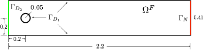
Figure 1: Test case 1: geometrical configuration, domain and boundaries [m].

Here we take $\rho=1$ kg/m³ as fluid density, and assign no-slip boundary conditions on $\Gamma_{1}$, a parabolic inflow profile

$$\mathbf{h}(\mathbf{x},t;\mu)=\left(\frac{4U(t,\mu)x_{2}(0.41-x_{2})}{0.41^{2}},0\right),\qquad\mbox{where }\ \ U(t;\mu)=\mu\sin(\pi t/8),$$ (13)

on the inlet $\Gamma_{D_{2}}$, and zero-stress Neumann conditions on the outlet $\Gamma_{N}$. We consider as parameter ($n_{\mu}=1$) $\mu\in\mathcal{P}=[1,2]$ m/s, which reflects on the Reynolds number varying in the range $[66,133]$. Equations (11) have been discretized in space by means of linear-quadratic $(\mathbb{P}_{2}-\mathbb{P}_{1}$), inf-sup stable, finite elements, and in time through a backward differentiation formula (BDF) of order 2 with semi-implicit treatment of the convective term (see, e.g., [61]) over the time interval $(0,T)$, with $T=8$ s, and a time-step $\Delta t=2\times 10^{-3}$ s. This strategy allows us to mitigate the computational cost associated to the use of a fully implicit BDF scheme, by linearizing the nonlinear convective terms; this latter task is realized by extrapolating the convective velocity through an extrapolation formula of the same order of the BDF introduced.

We already analyzed this test case in [42], where we were interested in approximating only the velocity field. Here we aim at assessing the performance of POD-DL-ROM neural network in approximating both the velocity and the pressure fields. In particular, we provide to the network data under the form of a tensor with 3 channels – that is, we set the dimension equal to $p=3$. The FOM dimension is equal to $N_{h}=[32446,32446,8239]$ (for the two velocity components and the pressure, respectively) and we select $N=256$ as dimension of the POD basis for each component of the solution. We choose $n=5$ as dimension of the nonlinear trial manifold $\tilde{S}_{n}$. We uniformly sample $N_{t}=400$ time instances and consider $N_{train}=21$ and $N_{test}=20$ training- and testing-parameter instances uniformly distributed over $\mathcal{P}$.

In Figure 2 and Figure 3 we compare the FOM and POD-DL-ROM pressure and velocity fields, these latter obtained with $n=5$, together with the relative error $\boldsymbol{\epsilon}_{k}$ in Figure 4, for the testing-parameter instance $\mu_{test}=1.975$ m/s ($Re=131$) at $t=1.062$ s and $t=4.842$ s. We highlight the ability of the POD-DL-ROM approximation to accurately capture the variability of the solution: indeed, in the case $t=1.062$ s (Figure 2) we do not assist to any vortex shedding; this latter is instead present in the case $t=4.842$ s (Figure 3), and is correctly reproduced.

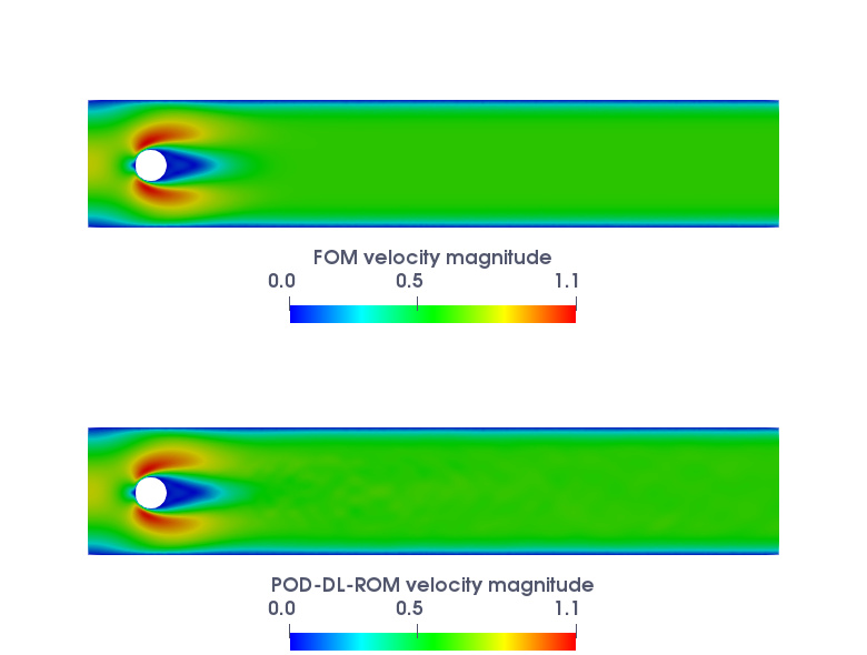
Figure 2: Test case 1: FOM and POD-DL-ROM solutions for the testing-parameter instance $\mu_{test}=1.975$ m/s at $t=1.062$ s, with $N=256$ and $n=5$. Left: velocity field magnitude; right: pressure field.

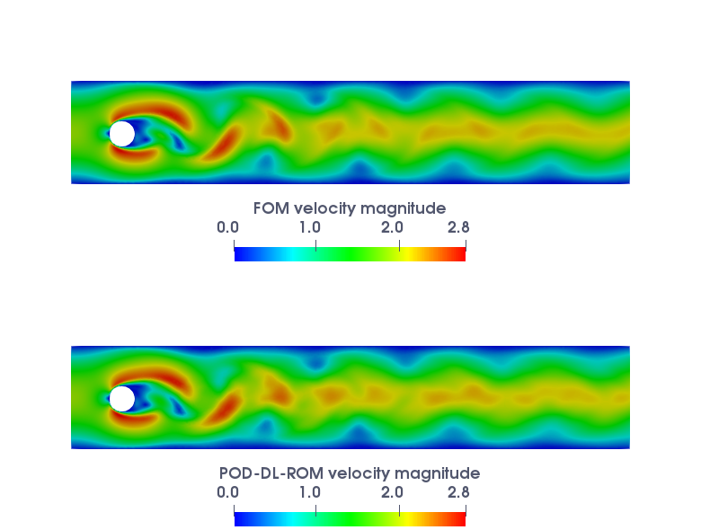
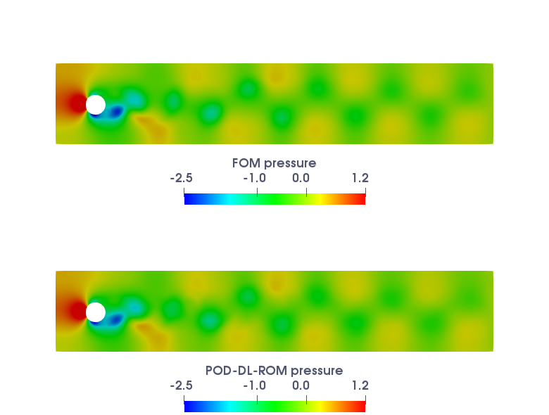
Figure 3: Test case 1: FOM and POD-DL-ROM solutions for the testing-parameter instance $\mu_{test}=1.975$ m/s at $t=4.842$ s, with $N=256$ and $n=5$. Left: velocity field magnitude; right: pressure field.

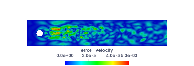
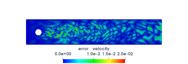
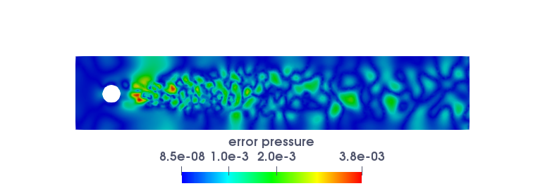
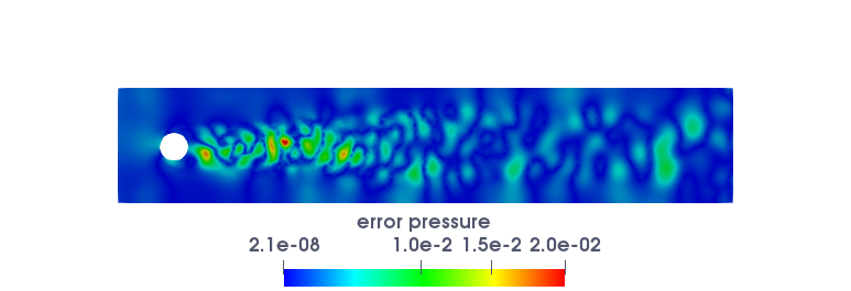
Figure 4: Test case 1: Relative errors $\epsilon_{k}$ for the testing-parameter instance $\mu_{test}=1.975$ m/s, with $N=256$ and $n=5$. Relative errors at $t=1.062$ s (left) and $t=4.842$ s (right) for velocity (left) and pressure (right).

To assess the ability of the POD-DL-ROM to provide accurate evaluations of output quantities of interest, we evaluate the drag and lift coefficients, related to the drag and lift forces around the circular obstacle; these are defined, in our case, as

$$F_{D}=\int_{\partial B_{r}}\Big{(}\nu\frac{\partial u_{2}}{\partial\eta}\eta_{2}-p\eta_{1}\Big{)}d\boldsymbol{\sigma},\qquad\textnormal{and}\qquad F_{L}=\int_{\partial B_{r}}\Big{(}\nu\frac{\partial u_{1}}{\partial\eta}\eta_{1}-p\eta_{2}\Big{)}d\boldsymbol{\sigma}.$$ (14)

where $\boldsymbol{\eta}=(\eta_{1},\eta_{2})^{T}$ denotes the (outward directed) normal unit vector to $\partial\Omega$. From (14), the dimensionless drag and lift coefficient can be obtained as

$$C_{D}=\frac{2}{U_{mean}^{2}L}F_{D},\qquad\textnormal{and}\qquad C_{L}=\frac{2}{U_{mean}^{2}L}F_{L},$$

where $U_{mean}$ is the parabolic input profile mean velocity.

The drag and lift coefficients coefficients computer over time by the FOM and the POD-DL-ROM, for the testing-parameter instances $\mu_{test}=1.975$ m/s, are reported in Figure 5. The POD-DL-ROM technique is also able to accurately capture the evolution of $C_{D}$ and $C_{L}$, related to the prescribed $\mu$-dependent input profile in (13), in both cases.

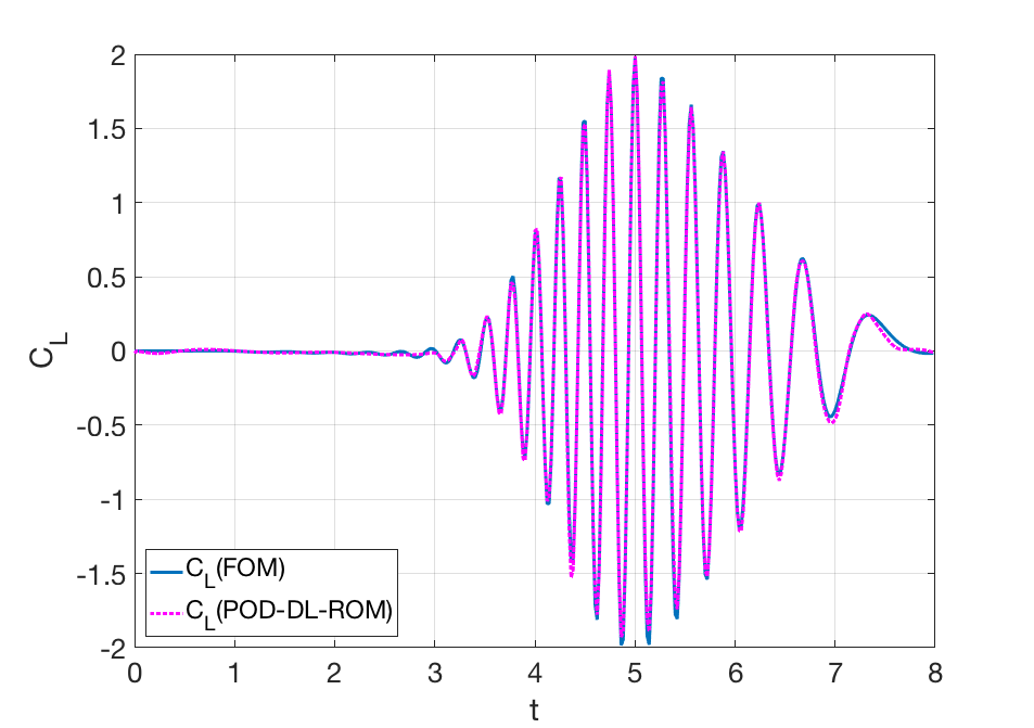
Figure 5: Test case 1: FOM and POD-DL-ROM drag (left) and lift (right) coefficients for the testing-parameter instance $\mu_{test}=1.975$.

Finally, the testing computational time, i.e. the time needed to compute $N_{t}$ time instances for an unseen testing-parameter instance, of the POD-DL-ROM on a GTX 1070 8GB GPU is given by 0.2 seconds, thus implying a speed-up equal to $1.25\times 10^{5}$ with respect to the time needed for the solution of the FOM.

3.2 Test case 2: fluid-structure interaction

We now focus on the case of a two-dimensional flow past an elastic beam attached to a fixed, rigid block [62, 63, 64] (see Figure 6 for a sketch of the geometry). The FSI model that we consider consists of a two-fields problem, where the incompressible Navier-Stokes equations written in the Arbitrary Lagrangian Eulerian (ALE) form for the fluid are coupled with the nonlinear elastodynamics equation modeling the solid deformation [53]. Because of the ALE approach we employ, a third non-physical geometry (or mesh motion) problem is introduced, which accounts for the fluid domain deformation and in turn defines the so-called ALE map.

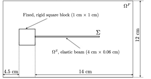
Figure 6: Test case 2: geometrical configuration and domains.

Let $\Omega^{F}$ and $\Omega^{S}$ be the domains occupied by the fluid and the solid, respectively, in their reference configuration. We denote by ${\color[rgb]{0,0,0}\Sigma}=\partial\Omega^{F}\cap\partial\Omega^{S}$ the fluid-structure interface on the reference configuration. At any time $t$, the domain occupied by the fluid $\Omega^{F}(t)$ can be retrieved from $\Omega^{F}$ by the ALE mapping

$$\mathcal{A}_{t}:\,\,\Omega^{F}\rightarrow\Omega^{F}(t),\qquad\mathbf{X}\mapsto\mathcal{A}_{t}(\mathbf{X})=\mathbf{X}+\mathbf{d}^{G}(\mathbf{X}),$$

where $\mathbf{d}^{G}(\mathbf{X})$ represents the displacement of the fluid domain. The coupled FSI problem thus consists in the following set of equations:

• Navier-Stokes in ALE form governing the fluid problem:

  $$\begin{cases}\displaystyle\rho^{F}\frac{\partial\mathbf{v}^{F}}{\partial t}\Big{|}_{\mathbf{X}}+(\mathbf{v}^{F}-\mathbf{w}^{G})\cdot\nabla\mathbf{v}^{F}-\nabla\boldsymbol{\sigma}^{F}(\mathbf{v}^{F},p^{F})=0&\quad\textnormal{in}\;\Omega^{F}(t),\\ \nabla\cdot\mathbf{v}^{F}=0&\quad\textnormal{in}\;\Omega^{F}(t);\end{cases}$$ (15)

• nonlinear elastodynamics equation governing the solid dynamics:

  $$\rho^{S}\frac{\partial\mathbf{d}^{S}}{\partial t^{2}}-\nabla\cdot\mathbf{P}(\mathbf{d}^{S})=0\qquad\textnormal{in}\;\Omega^{S};$$ (16)

• coupling at the FS interface $\Sigma$:

  $$\begin{cases}\displaystyle\mathbf{v}^{F}=\frac{\partial\mathbf{d}^{S}}{\partial t},\\ \boldsymbol{\sigma}^{F}(\mathbf{v}^{F},p^{F})\mathbf{n}^{F}+\boldsymbol{\sigma}^{S}(\mathbf{d}^{S})\mathbf{n}^{S}={\bf 0};\end{cases}$$ (17)

• linear elasticity equations modeling the mesh motion problem:

  $$\begin{cases}\displaystyle-\nabla\cdot\boldsymbol{\sigma}^{G}(\mathbf{d}^{G})=0&\quad\textnormal{in}\;\Omega^{F},\\ \mathbf{d}^{G}=\mathbf{d}^{S}&\quad\textnormal{on}\;\Sigma,\end{cases}$$ (18)

where $\boldsymbol{\sigma}^{F}(\mathbf{v}^{F},p^{F})=-p^{F}\mathbf{I}+2\mu^{F}\boldsymbol{\epsilon}(\mathbf{v}^{F})$ is the fluid Cauchy stress tensor, $\boldsymbol{\sigma}^{S}(\mathbf{d}^{S})=J^{-1}\mathbf{P}\mathbf{F}^{T}$ is the solid Cauchy stress tensor, $\mathbf{F}={\bf I}+\nabla{\bf d}^{S}$ is the deformation tensor, and

$$\mathbf{w}^{G}=\frac{\partial\mathbf{d}^{G}}{\partial t}\Big{|}_{\mathbf{X}}$$

is the fluid mesh velocity. See, e.g., [53] for further details about the FSI model.

Both fluid and solid equations are complemented by appropriate initial and boundary conditions. In particular, the lateral boundaries are assigned zero normal velocity and zero tangential stress. Zero-traction boundary condition is applied at the outflow. The flow is driven by a uniform inflow velocity of 51.3 cm/s. Zero-initial conditions are assigned both for the fluid and the solid equations. The fluid density and viscosity are $1.18\times 10^{-3}$ g/cm³ and $1.82\times 10^{-4}$ g/(cm $\cdot$ s) respectively, resulting in a Reynolds number of 100 based on the edge length of the block. The beam is modeled as a solid made of the neo-Hookean material and the density of the beam is 0.1 g/cm³.

The field equations are discretized in space and time using: matching spatial discretizations between fluid and structure at the interface; SUPG stabilized linear finite elements ($(\mathbb{P}_{1}-\mathbb{P}_{1}$) and a BDF of order 2 in time for the fluid subproblem; the same finite element space as for the fluid velocity for both the fluid displacement subproblem and the structural subproblem, and the Newmark scheme in time for this latter. The resulting nonlinear problem is solved through a monolithic geometry-convective explicit (GCE) scheme, obtained by linearizing the fluid convective term (with a BDF extrapolation) and treating the geometry problem explicitly [65, 66]. Here $n_{\mu}=2$ parameters are considered, the Young modulus $\mu_{1}$ and the Poisson ratio $\mu_{2}$, varying in the parameter space $\mathcal{P}=10^{6}\cdot[2.3,2.7]\;\textnormal{g/(cm $\cdot$ s${}^{2}$)}\times[0.3,0.4]$. We build a FOM considering $N_{h}=[16452,8226,1974]$ DOFs for the velocity, the pressure and the displacement fields, respectively, and a time step $\Delta t=1.65\times 10^{-3}$ over $(0,T)$ with $T=3$ s.

Regarding the construction of the proposed POD-DL-ROM, for the training of the neural networks, we uniformly sample $N_{t}=606$ time instances and $N_{train}=5\times 3=15$ training-parameter instances, uniformly distributed in each parametric direction. At testing phase, $N_{test}=4\times 2=8$ testing-parameter instances, different from the training ones, have been considered. The maximum number of epochs is set equal to $N_{epochs}=20000$, the batch size is $N_{b}=40$ and, regarding the early-stopping criterion, we stop the training if the loss function does not decrease within 500 epochs. We are interested in reconstructing the velocity and the displacement fields, so we set the number of channels to $p=2d=4$ and we recall the ability of the POD-DL-ROM neural network to handle different FOM dimensions $N_{h,i}$, for $i=1,\ldots,p$, that is only the POD dimension must be equal among the different fields considered. Moreover, we set $N=256$ as dimension of the POD basis, and $n=5$ as dimension of the reduced nonlinear trial manifold. The training and testing phases of the POD-DL-ROM neural network have been performed on a Tesla V100 32GB GPU.

In Figure 7 we report the FOM and the POD-DL-ROM velocity magnitudes, the latter with $N=256$ and $n=5$, for two testing-parameter instances – $\boldsymbol{\mu}_{test}=[2.3\times 10^{6}\textnormal{ g/(cm $\cdot$ s${}^{2}$)},0.325]$ and $\boldsymbol{\mu}_{test}=[2.7\times 10^{6}\textnormal{ g/(cm $\cdot$ s${}^{2}$)},0.375]$ – at $t=2.3084$ s and $t=2.64$ s.

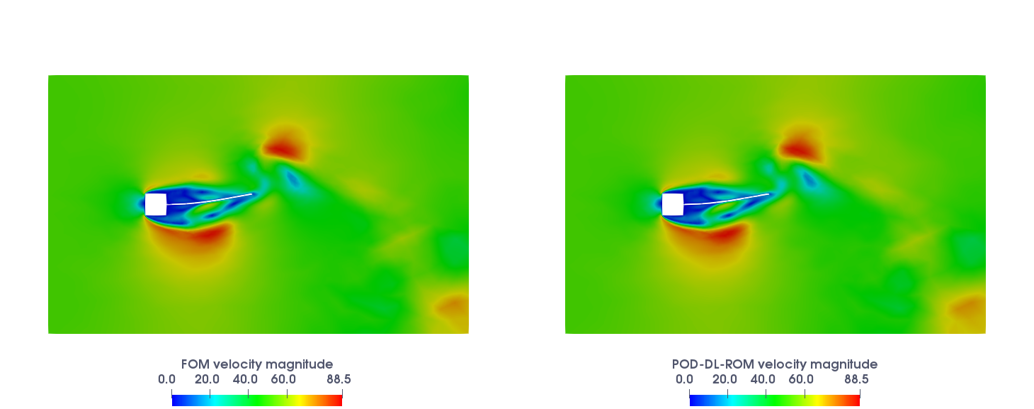
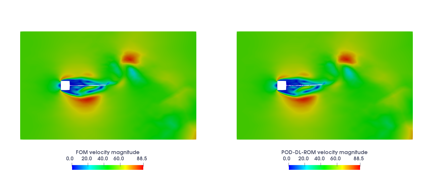
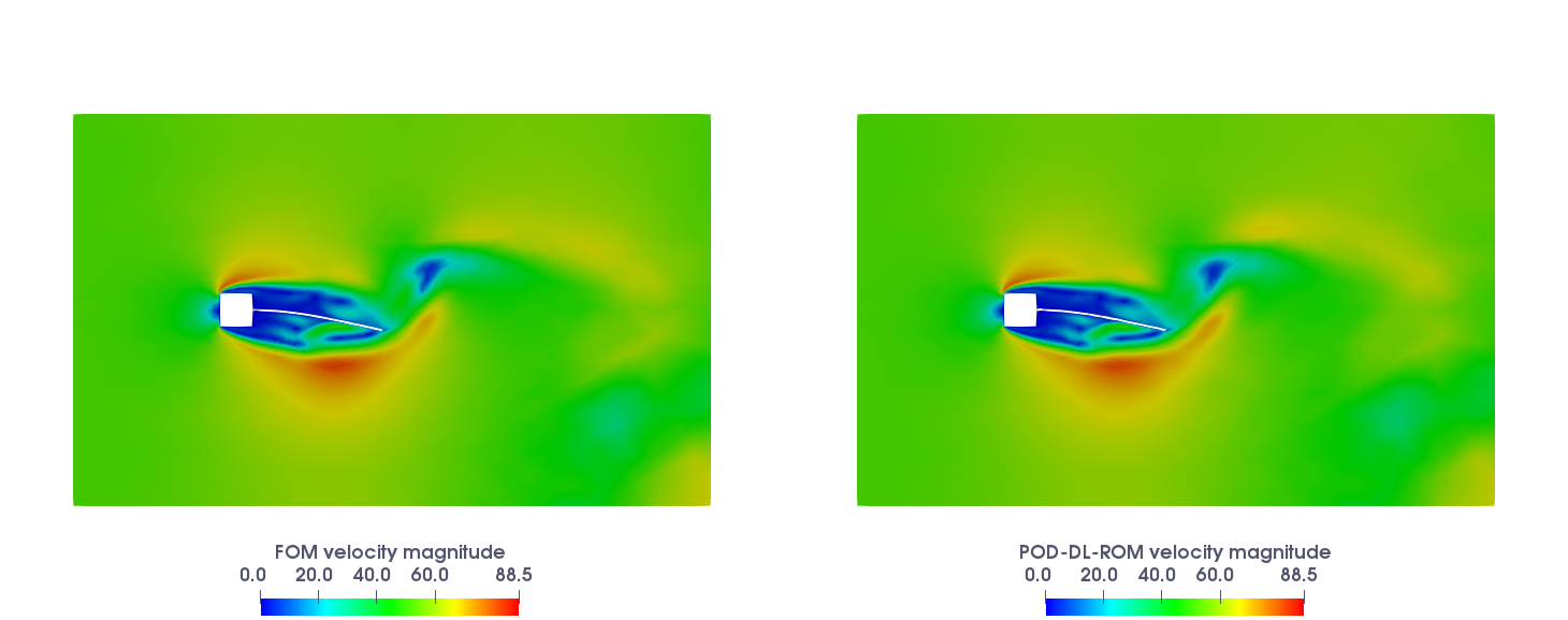
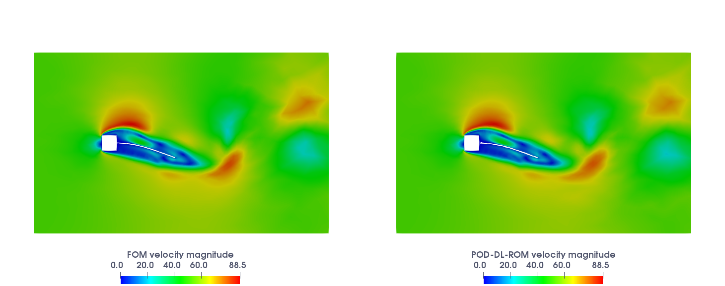
Figure 7: Test case 2: FOM and POD-DL-ROM fluid velocity magnitudes for the testing-parameter instances $\boldsymbol{\mu}_{test}=[2.3\times 10^{6}\textnormal{ g/(cm $\cdot$ s${}^{2}$)},0.325]$ at $t=2.3084$ s and $t=2.64$ s (first and second row) and $\boldsymbol{\mu}_{test}=[2.7\times 10^{6}\textnormal{ g/(cm $\cdot$ s${}^{2}$)},0.375]$ at $t=2.3084$ s and $t=2.64$ s (third and fourth row).

We point out that the dependence of the displacement field on the parameters reflects on the velocity field by producing a strong variability over the parameter space, which is accurately captured by the POD-DL-ROM solutions. The FOM and POD-DL-ROM displacement magnitudes, for the testing-parameter instances $\boldsymbol{\mu}_{test}=[2.3\times 10^{6}\textnormal{ g/(cm $\cdot$ s${}^{2}$)},0.325]$ and $\boldsymbol{\mu}_{test}=[2.7\times 10^{6}\textnormal{ g/(cm $\cdot$ s${}^{2}$)},0.375]$ at $t=2.3084$ s and $t=2.64$ s over the domain, are shown in Figure 8. The comparison between the FOM and POD-DL-ROM displacement magnitudes, for the testing-parameter instance $\boldsymbol{\mu}_{test}=[2.7\times 10^{6}\textnormal{ g/(cm $\cdot$ s${}^{2}$)},0.375]$ at $\mathbf{x}^{*}=(5.50,6.07)$ cm over time, is reported in Figure 8, from which it is clearly visible that the POD-DL-ROM is also able to capture the main features of the elastic beam dynamics.

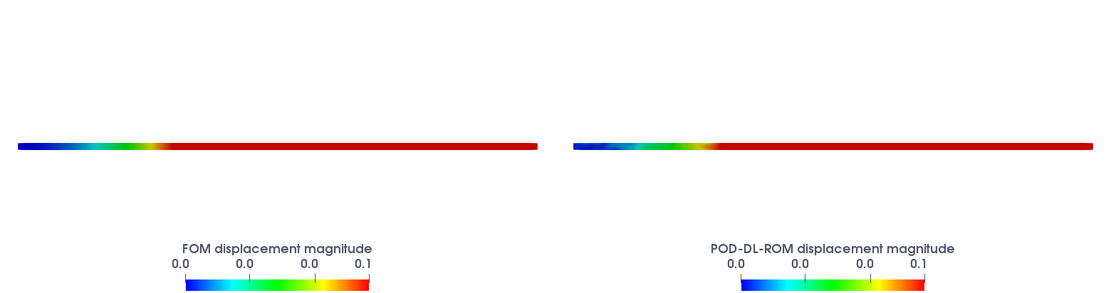
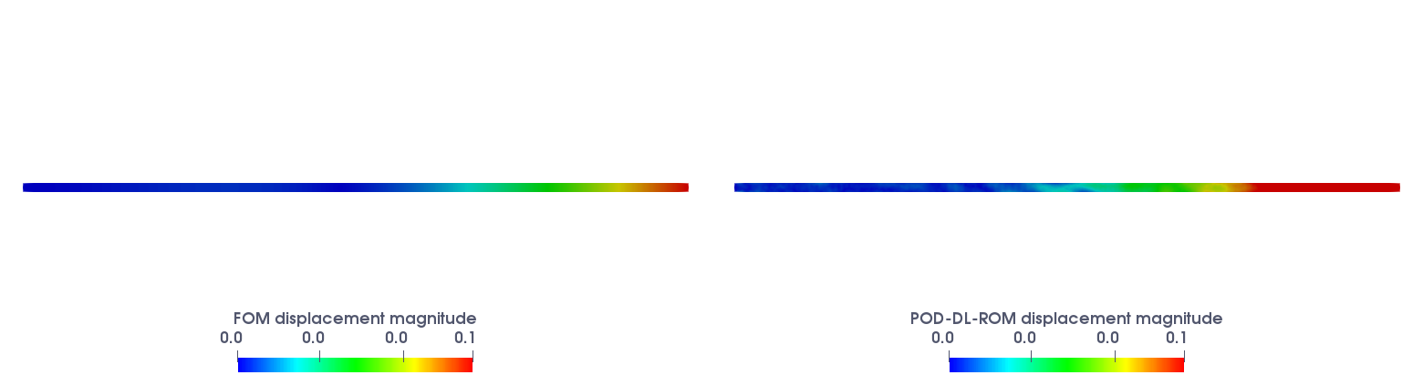
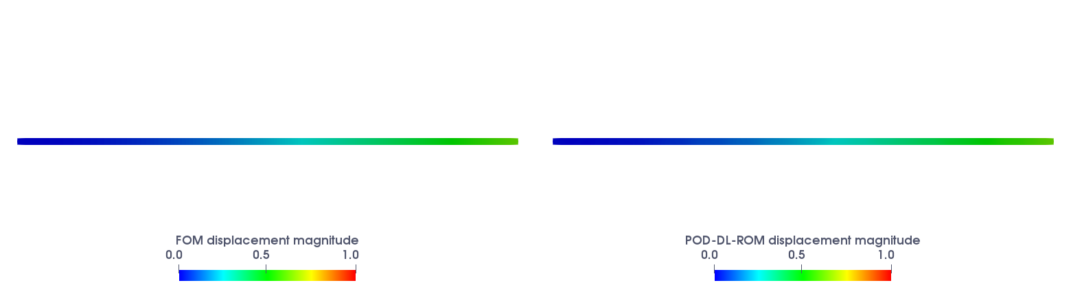
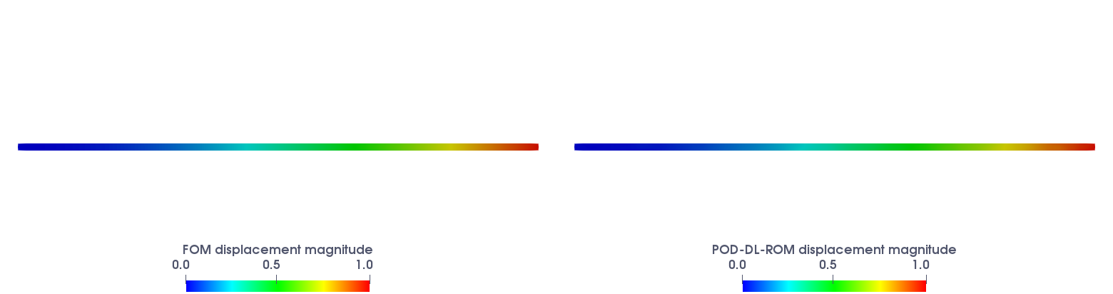
Figure 8: Test case 2: FOM and POD-DL-ROM structure displacement magnitudes for the testing-parameter instances $\boldsymbol{\mu}_{test}=[2.3\times 10^{6}\textnormal{ g/(cm $\cdot$ s${}^{2}$)},0.325]$ at $t=2.3084$ s and $t=2.64$ s (first and second row) and $\boldsymbol{\mu}_{test}=[2.7\times 10^{6}\textnormal{ g/(cm $\cdot$ s${}^{2}$)},0.375]$ at $t=2.3084$ s and $t=2.64$ s (third and fourth row).

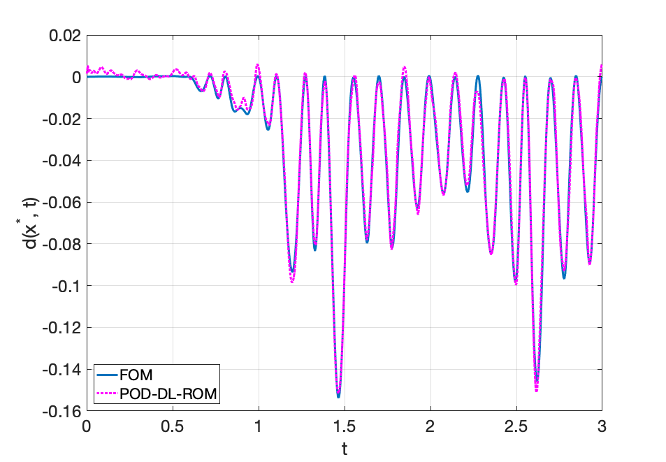
Figure 9: Test case 2: FOM and POD-DL-ROM displacement at $\mathbf{x}^{*}=(5.50,6.07)$ cm for the testing-parameter instance $\boldsymbol{\mu}_{test}=[2.7\times 10^{6}\textnormal{ g/(cm $\cdot$ s${}^{2}$)},0.375]$.

Finally, in Table 3 we report the POD-DL-ROM GPU training (including validation) time, the testing time, i.e. the time needed to compute $N_{t}$ time instances for a testing-parameter instance, and the time required to compute one time instance at testing time. Indeed, we recall that the DL-ROM solution can be queried at a given time without requiring the solution of a dynamical system to recover the former time instances. We also show the speed-up gained by the POD-DL-ROM with respect to the CPU time needed to solve the FOM.

Table 3: Test case 2: POD-DL-ROM GPU computational times.

training time [h] testing time [s] 1-sample testing time [s] speed-up 7 $4\times 10^{-2}$ $5\times 10^{-3}$ $1.77\times 10^{5}$ ($1.41\times 10^{6}$)

3.3 Test case 3: blood flow in a cerebral aneurysm

In this last test case we consider the fast simulation of blood flows in a cerebral (or intracranial) aneurysm, that is, a localized dilation or ballooning of a blood vessel in the brain, often occurring in the circle of Willis, the vessel network at the base of the brain. Blood velocity and pressure, wall shear stress (WSS), blood flow impingement and particle residence time all play a key role in the growth and rupture of cerebral aneurysms – see e.g. [67, 68, 69] – which might ultimately yield potentially severe brain damages. For these reasons, computational haemodynamics inside aneurysm models can provide output quantities of interest useful for planning their surgical treatment.

We consider the artery aneurysm shown in Figure 10 (left), and extracted from the Aneurisk dataset repository [70, 71, 72]. We consider blood as a Newtonian fluid, with constant viscosity, and a rigid arterial wall, so that blood flow dynamics can be described by the following Navier-Stokes equations:

$$\left\{\begin{aligned} &\rho\frac{\partial\mathbf{v}}{\partial t}+\rho\mathbf{v}\cdot\nabla\mathbf{v}-\nabla\cdot\boldsymbol{\sigma}(\mathbf{v},p)=\mathbf{0}&\qquad&(\mathbf{x},t)\in\Omega^{F}\times(0,T),\\ &\nabla\cdot\mathbf{v}=0&\qquad&(\mathbf{x},t)\in\Omega^{F}\times(0,T),\\ &\mathbf{v}=\mathbf{0}&\qquad&(\mathbf{x},t)\in\Gamma_{w}\times(0,T),\\ &\mathbf{v}=k\mathbf{v}_{in}Q(t)&\qquad&(\mathbf{x},t)\in\Gamma_{D}\times(0,T),\\ &\boldsymbol{\sigma}(\mathbf{v},p)\mathbf{n}=\mathbf{0}&\qquad&(\mathbf{x},t)\in\Gamma_{N}\times(0,T),\\ &\mathbf{v}(0)=\mathbf{0}&\qquad&\mathbf{x}\in\Omega,\ t=0,\end{aligned}\right.$$ (19)

where the stress tensor is defined as in (12). On the arterial wall $\Gamma_{w}$ a no-slip condition on the fluid velocity is imposed, flow resistance at the outlet boundaries $\Gamma_{N}$ is neglected, while a parabolic profile $\mathbf{v}_{in}$ is specified at the lumen inlet, where the parametrization of the inlet flow rate profile $Q(t;\boldsymbol{\mu})$ has been obtained by interpolating with radial basis functions a base profile $Q(t)$ taken from [73], and then treating some of the interpolated values as parameters (see Figure 10, right), see [74] for further details.

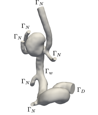
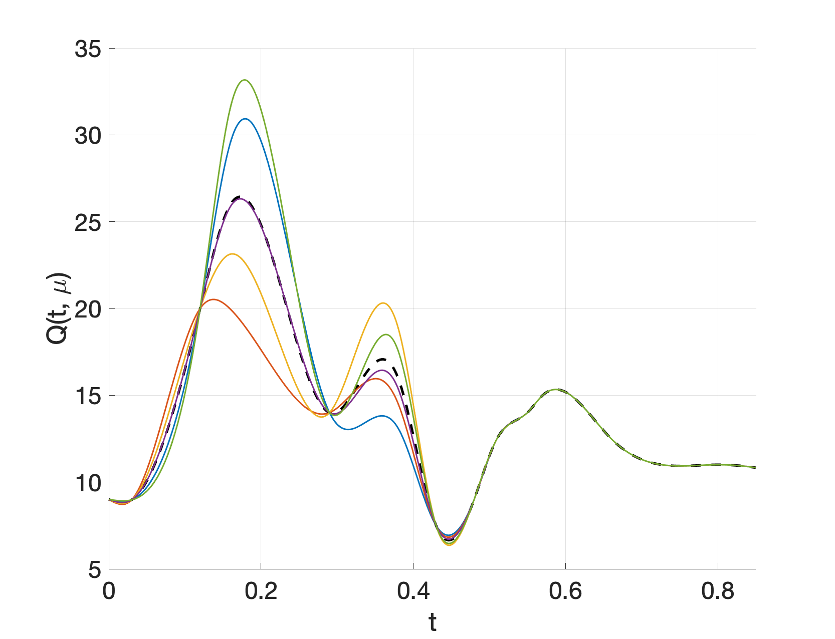
Figure 10: Test case 3. Left: aneurysm geometry. Right: inlet flow rate $Q(t;\boldsymbol{\mu})$ during the heart cycle for different parameter values; the black dashed curve corresponds to the base profile $Q(t)$.

In particular, we consider $n_{\mu}=2$ parameters $\boldsymbol{\mu}\in\mathcal{P}\subset\mathbb{R}^{2}$ such that the flow rate at $t=0.16$ s and $t=0.38$ s admits variations up to 15$\%$ of the reference value. A comparison between some flow rate profiles corresponding to different parameter values is shown in Figure 10, right. The scaling factor $k$ in (19) is such that

$$\int_{\Gamma_{D}}k\mathbf{v}_{in}\cdot\mathbf{n}d\sigma=1.$$

Blood dynamic viscosity $\nu=0.035$ P and density are set to $\rho=1$ g/cm³, respectively.

Concerning the FOM discretization, we employ a SUPG-BDF semi-implicit time scheme of order 2 with linear finite elements for both velocity and pressure variables. We employ a time-step $\Delta t=10^{-3}$ over the interval $(0,T)$ with $T=0.85$ s. We simulate the blood flow starting from an initial condition obtained by solving the steady Stokes problem. We are interested in reconstructing the blood velocity field, so we set the FOM dimensions to $N_{h}=[41985,41985,41985]$, and $p=3$. The POD dimension is equal to $N=64$, for each component of the solution, and the dimension of the reduced nonlinear trial manifold is chosen to be equal to $n=5$, very close to the intrinsic dimension of the problem $n_{\mu}+1=3$. We consider $N_{t}=850$ time instances, $N_{train}=6$, and $N_{test}=3$ training- and testing-parameter instances, sampled over $\mathcal{P}$ by means of the latin hypercube sampling strategy.

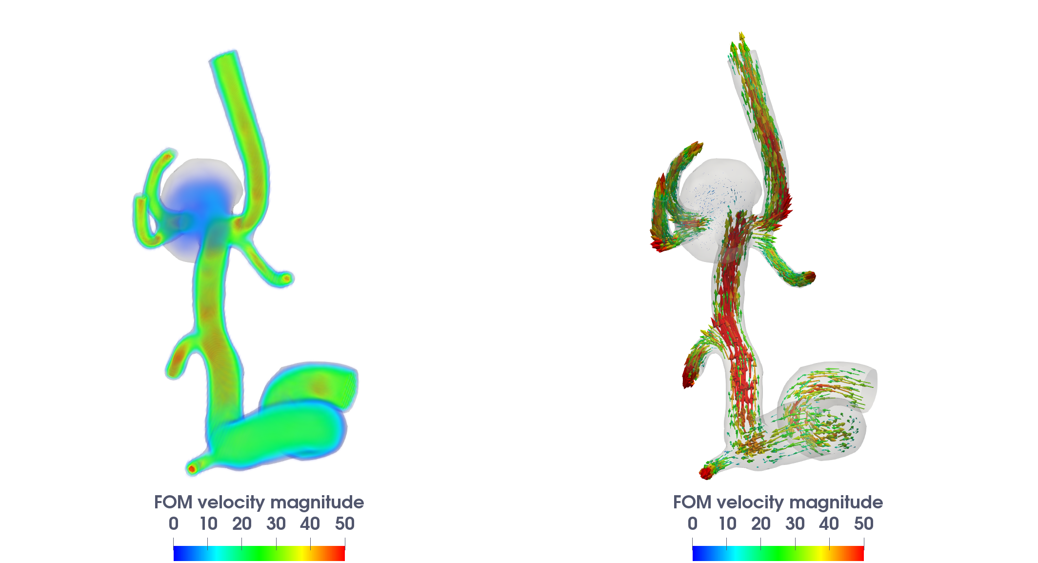
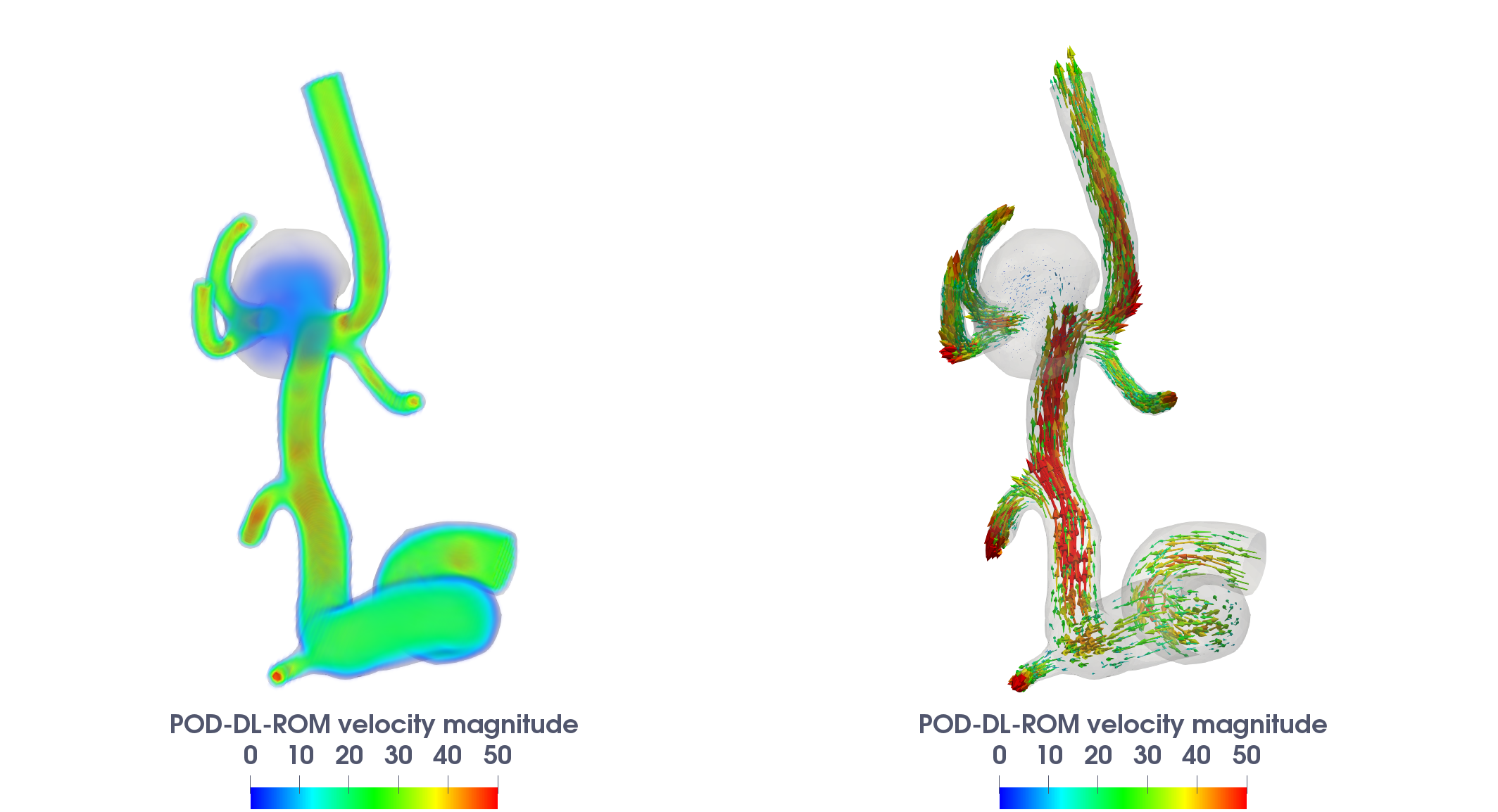
Figure 11: Test case 3: FOM (top) and POD-DL-ROM (bottom) velocity fields for the testing-parameter instance $\boldsymbol{\mu}_{test}=(5.9102,3.1179)$ at the systolic peak $t=0.18$ s.

In Figure 11 we compare the FOM and POD-DL-ROM velocity field magnitudes, the latter obtained with $N=64$ and $n=5$, for the testing-parameter instance $\boldsymbol{\mu}_{test}=(5.9102,3.1179)$ at the systolic peak $t=0.18$ s, along with the relative error $\boldsymbol{\epsilon}_{k}$ reported in Figure 12. By looking at the pattern and the magnitude of the vector velocity field in Figure 11, it is evident that the abnormal bulge and the inlet are the portions of the domain where the blood flow velocity is smaller, and we remark the ability of the POD-DL-ROM technique in capturing such dynamics in an extremely detailed manner.

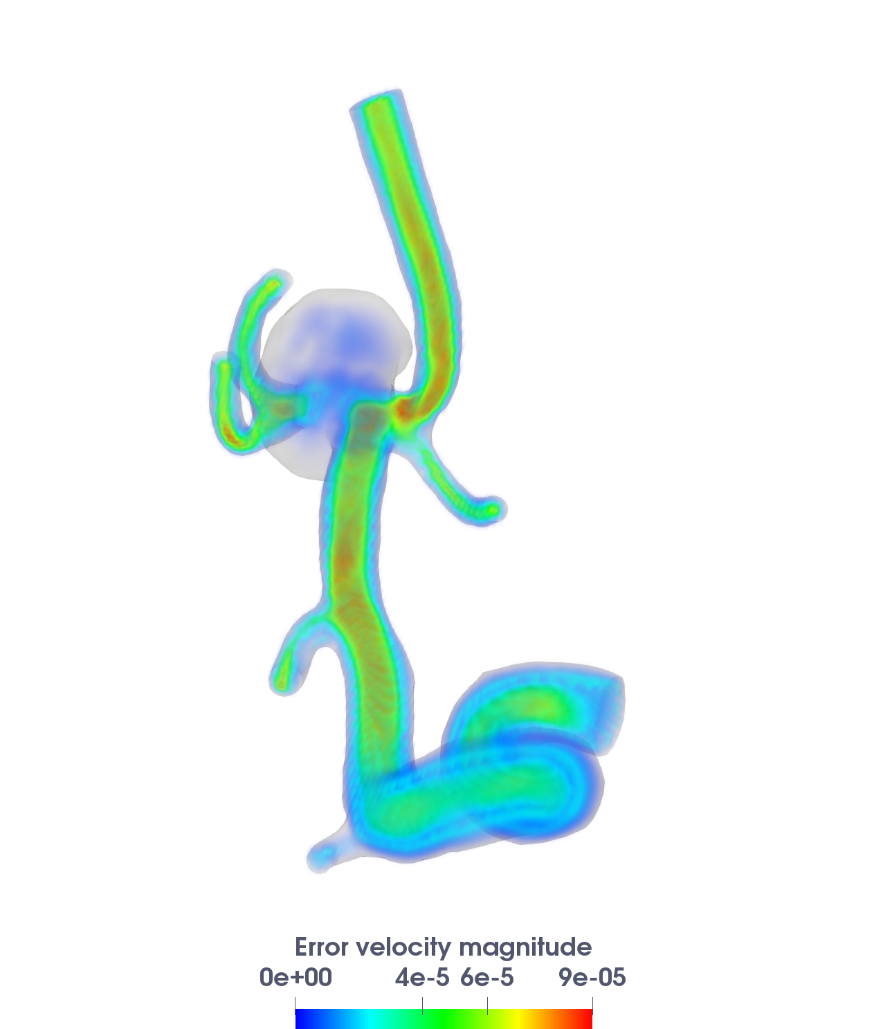
Figure 12: Test case 3: Relative error in the velocity magnitude for the testing-parameter instance $\boldsymbol{\mu}_{test}=(5.9102,3.1179)$ at the systolic peak $t=0.18$ s.

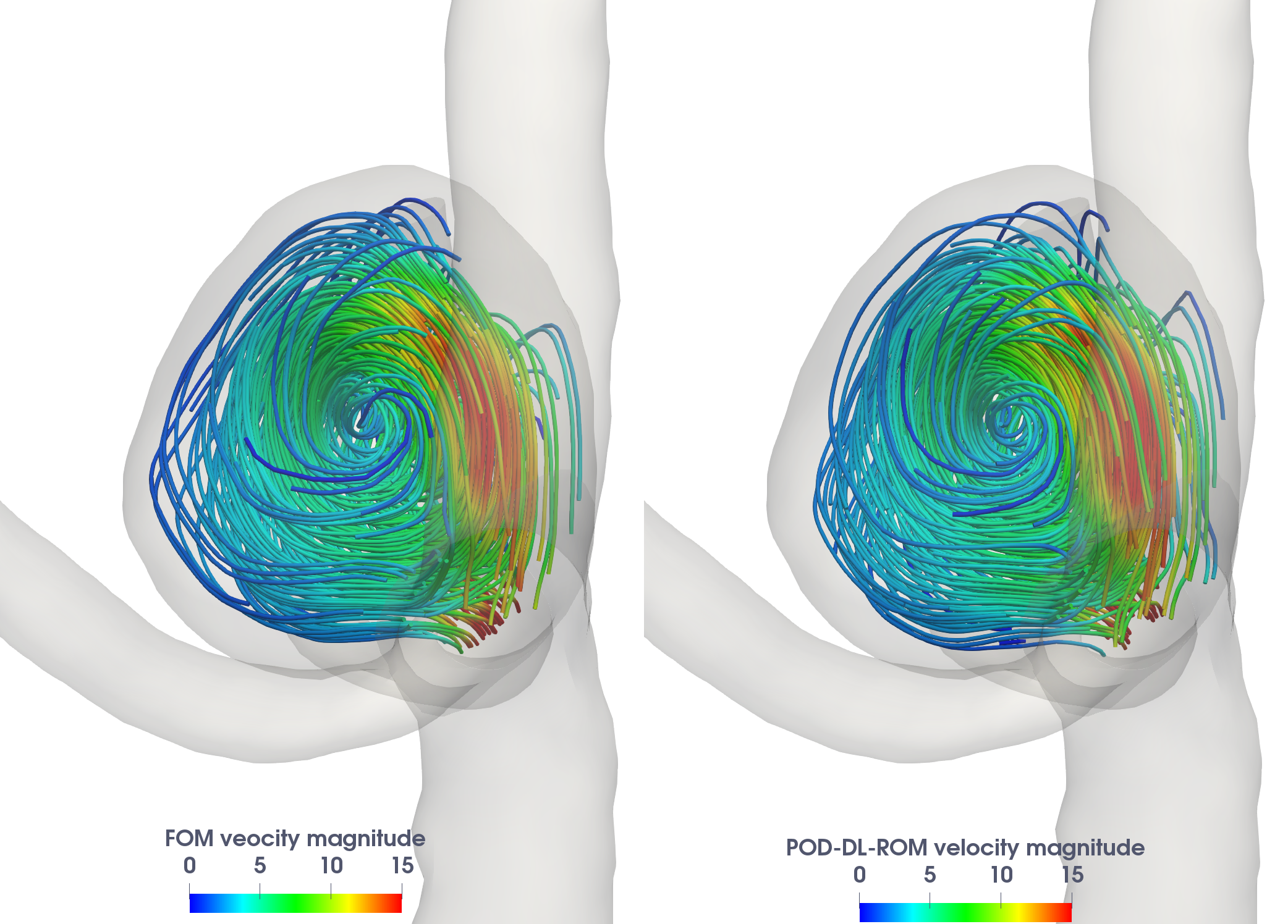
Figure 13: Test case 3: FOM (left) and POD-DL-ROM (right) velocity magnitude streamlines for the testing-parameter instance $\boldsymbol{\mu}_{test}=(5.9102,3.1179)$ at the sistolic peak $t=0.5$ s.

In Figure 13 we report the streamlines of the blood velocity field, obtained with the FOM and the POD-DL-ROM, for the testing-parameter instance $\boldsymbol{\mu}_{test}=(5.9102,3.1179)$ at $t=0.5$ s. In Figure 14 we report instead a detailed view of the pattern of the fluid velocity field obtained for the testing-parameter instance $\boldsymbol{\mu}_{test}=(5.9102,3.1179)$ at $t=0.18$ s, highlighting the recirculation of the flow in the bulge and the blood stasis in this region.

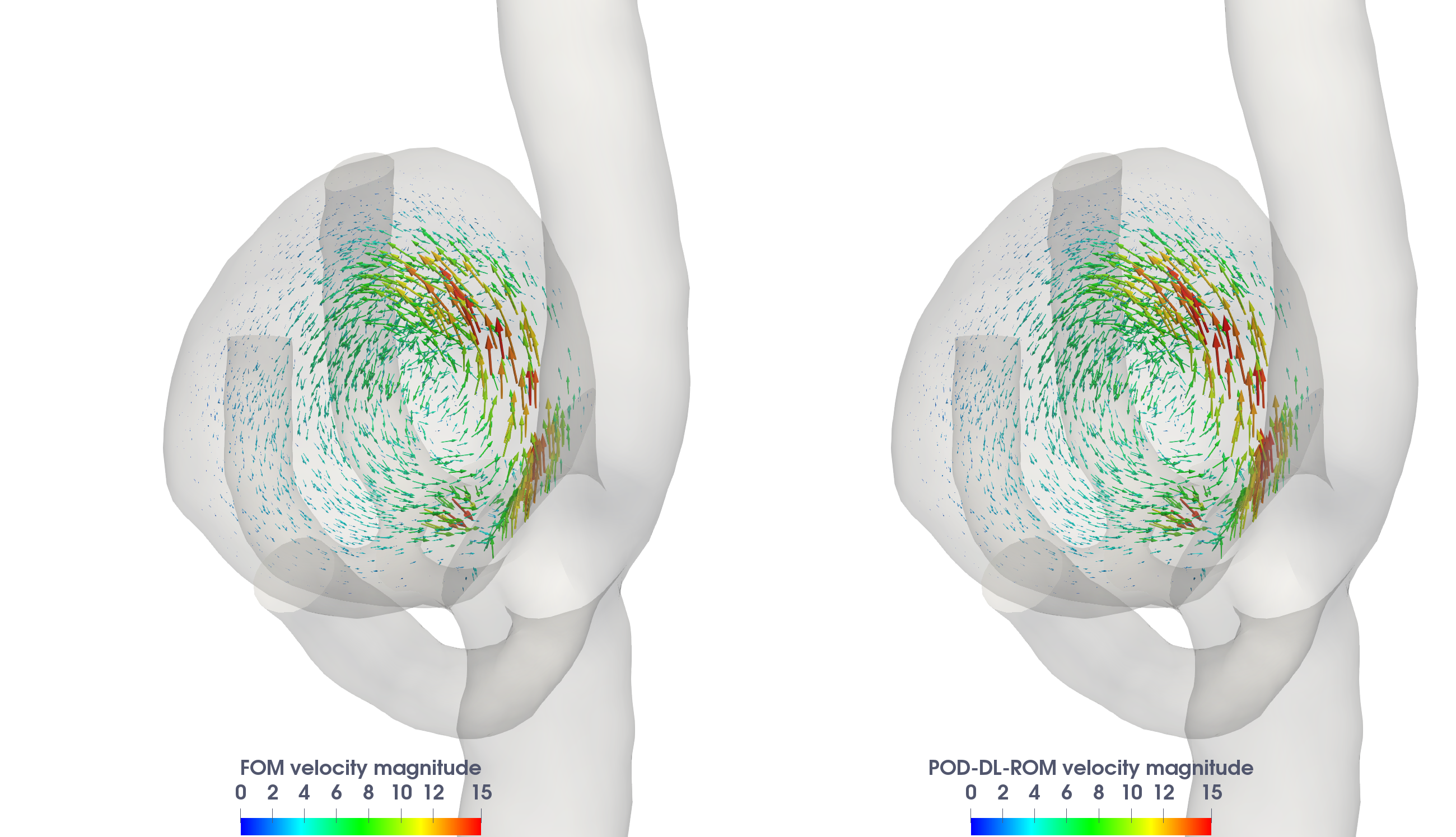
Figure 14: Test case 3: FOM (left) and POD-DL-ROM (right) velocity field magnitude for the testing-parameter instance $\boldsymbol{\mu}_{test}=(5.9102,3.1179)$ at $t=0.18$ s.

Finally, the testing computational time, i.e. the time needed to compute $N_{t}$ time instances for an unseen testing-parameter instance, of the POD-DL-ROM on a Tesla V100 32GB GPU is given by 0.28 seconds, thus implying a speed-up equal to $3.98\times 10^{5}$ with respect to the time needed for the solution of the FOM, and the possibility to obtain a fully detailed simulation of a complex blood flow in real-time.

4 Discussion

In this work, we have taken advantage of a recently proposed technique [42] to build non-intrusive low-dimensional ROMs by exploiting DL algorithms to handle fluid dynamics problems. This strategy allows us to overcome some drawbacks of classical projection-based ROM techniques arising when they are applied to incompressible flow simulations.

In particular, POD-DL-ROMs overcome the need of:

• treating efficiently nonlinearities and (nonaffine) parameter dependencies, thus avoiding expensive and intrusive hyper-reduction techniques;

• approximating both velocity and pressure fields, in those cases where one might be interested only in the visualization of a single field;

• imposing physical constraints that couple different submodels, as in the case of fluid-structure interaction (the different field variables are indeed treated as independent by the neural network);

• ensuring the ROM stability by enriching the reduced basis spaces;

• solving a dynamical system at the reduced level to model the fluid dynamics, however keeping the error propagation in time under control.

We assessed the performance of the POD DL-ROM technique on three test cases, dealing with the flow around a cylinder benchmark, the fluid-structure interaction between an elastic beam attached to a fixed, rigid block and a laminar incompressible flow, and the blood flow in a cerebral aneurysm, by showing its ability in providing accurate and efficient (even on moderately large-scale problems) ROMs, which multi-query and real-time applications may ultimately rely on. In particular, the prior dimensionality reduction performed through POD on the snapshot matrices also enhances the overall efficiency of the technique during the offline training stage.

Therefore, we can conclude that POD-DL-ROMs provide a non-intrusive and general-purpose tool enabling us to perform real-time numerical simulations of fluid flows. Since they return a (FOM-like detailed) computation of the field variables, rather than approximating selected output quantities of interest as in the case of traditional emulators or surrogate models, POD-DL-ROMs are a viable tool for detailed flow analysis, without any requirement in terms of computational resources during the online testing stage.

Authors’ Contributions

Conceptualization: S.F. and A.M.; Formal analysis: S.F.; Funding acquisition: A.M.; Investigation: S.F.; Methodology: S.F. and A.M.; Software: S.F.; Supervision: A.M.; Validation: S.F.; Visualization: S.F.; Writing: S.F. and A.M. .

References

- Quarteroni et al. [2017] A. Quarteroni, A. Manzoni, C. Vergara, The cardiovascular system: mathematical modelling, numerical algorithms and clinical applications, Acta Numerica 26 (2017) 365–590.
- Quarteroni et al. [2016] A. Quarteroni, A. Manzoni, F. Negri, Reduced Basis Methods for Partial Differential Equations: An Introduction, Springer, 2016.
- Kunisch and Volkwein [2002] K. Kunisch, S. Volkwein, Galerkin proper orthogonal decomposition methods for a general equation in fluid dynamics, SIAM J. Numer. Anal. 40 (2002) 492–515.
- Gunzburger et al. [2007] M. D. Gunzburger, J. S. Peterson, J. N. Shadid, Reducer-order modeling of time-dependent PDEs with multiple parameters in the boundary data, Comput. Methods Appl. Mech. Engrg. 196 (2007) 1030–1047.
- Bergmann et al. [2009] M. Bergmann, C.-H. Bruneau, A. Iollo, Enablers for robust POD models, J. Comput. Phys. 228 (2009) 516 – 538.
- Weller et al. [2010] J. Weller, E. Lombardi, M. Bergmann, A. Iollo, Numerical methods for low-order modeling of fluid flows based on POD, Int. J. Numer. Methods Fluids 63 (2010) 249–268.
- Ballarin et al. [2015] F. Ballarin, A. Manzoni, A. Quarteroni, G. Rozza, Supremizer stabilization of POD–Galerkin approximation of parametrized steady incompressible Navier–Stokes equations, Int. J. Numer. Methods Engng. 102 (2015) 1136–1161.
- Dal Santo and Manzoni [2019] N. Dal Santo, A. Manzoni, Hyper-reduced order models for parametrized unsteady navier-stokes equations on domains with variable shape, Adv. Comput. Math. 45 (2019) 2463–2501.
- Veroy and Patera [2005] K. Veroy, A. Patera, Certified real-time solution of the parametrized steady incompressible Navier-Stokes equations: rigorous reduced-basis a posteriori error bounds, International Journal for Numerical Method in Fluids 47(8-9) (2005) 773–788.
- Deparis [2008] S. Deparis, Reduced basis error bound computation of parameter-dependent Navier–Stokes equations by the natural norm approach, SIAM J. Numer. Anal. 46 (2008) 2039–2067.
- Manzoni [2014] A. Manzoni, An efficient computational framework for reduced basis approximation and a posteriori error estimation of parametrized Navier-Stokes flows, ESAIM Math. Modelling Numer. Anal. 48 (2014) 1199–1226.
- Yano [2014] M. Yano, A space-time petrov–galerkin certified reduced basis method: Application to the Boussinesq equations, SIAM J. Sci. Comput. 36 (2014) A232–A266.
- Lassila et al. [2014] T. Lassila, A. Manzoni, A. Quarteroni, G. Rozza, Model order reduction in fluid dynamics: challenges and perspectives, in: A. Quarteroni, G. Rozza (Eds.), Reduced Order Methods for Modeling and Computational Reduction, volume 9 of Modeling, Simulation and Applications (MS&A), Springer International Publishing, Switzerland, 2014, pp. 235–274.
- Carlberg et al. [2013] K. Carlberg, C. Farhat, J. Cortial, D. Amsallem, The GNAT method for nonlinear model reduction: effective implementation and application to computational fluid dynamics and turbulent flows, J. Comput. Phys. 242 (2013) 623–647.
- Caiazzo et al. [2014] A. Caiazzo, T. Iliescu, V. John, S. Schyschlowa, A numerical investigation of velocity–pressure reduced order models for incompressible flows, J. Comput. Phys. 259 (2014) 598–616.
- Carlberg et al. [2011] K. Carlberg, C. Bou-Mosleh, C. Farhat, Efficient non-linear model reduction via a least-squares Petrov–Galerkin projection and compressive tensor approximations, Int. J. Numer. Methods Engng. 86 (2011) 155–181.
- Baiges et al. [2013] J. Baiges, R. Codina, S. Idelsohn, Explicit reduced-order models for the stabilized finite element approximation of the incompressible Navier-Stokes equations, Int. J. Numer. Meth. Fluids 72 (2013) 1219–1243.
- Rozza et al. [2013] G. Rozza, D. Huynh, A. Manzoni, Reduced basis approximation and error bounds for Stokes flows in parametrized geometries: roles of the inf–sup stability constants., Numer. Math. 125 (2013) 115–152.
- Dal Santo et al. [2019] N. Dal Santo, S. Deparis, A. Manzoni, A. Quarteroni, An algebraic least squares reduced basis method for the solution of parametrized Stokes equations, Comput. Meth. Appl. Mech. Engrg. 344 (2019) 186–208.
- Lassila et al. [2013] T. Lassila, A. Manzoni, A. Quarteroni, G. Rozza, A reduced computational and geometrical framework for inverse problems in hemodynamics, Int. J. Numer. Methods Biomed. Engng. 29 (2013) 741–776.
- Colciago et al. [2014] C. Colciago, S. Deparis, . Quarteroni, Comparisons between reduced order models and full 3D models for fluid–structure interaction problems in haemodynamics, J. Comput. Appl. Math. 265 (2014) 120–138.
- Brunton et al. [2020] S. Brunton, B. Noack, P. Koumoutsakos, Machine learning for fluid mechanics, Ann. Rev. Fluid Mech. 52 (2020) 477–508.
- Kutz [2017] J. Kutz, Deep learning in fluid dynamics, J. Fluid Mech. 814 (2017) 1–4.
- Ströfer et al. [2019] C. Ströfer, J.-L. Wu, H. Xiao, E. Paterson, Data-driven, physics-based feature extraction from fluid flow fields using convolutional neural networks, Commun. Comput. Phys. 25 (2019) 625–650.
- Lye et al. [2020] K. Lye, S. Mishra, D. Ray, Deep learning observables in computational fluid dynamics, J. Comput. Phys. 410 (2020) 109339.
- Bhatnagar et al. [2019] S. Bhatnagar, Y. Afshar, S. Pan, K. Duraisamy, S. Kaushik, Prediction of aerodynamic flow fields using convolutional neural networks, Comp. Mech. 64 (2019) 525–545.
- Thuerey et al. [2020] N. Thuerey, K. Weißenow, L. Prantl, X. Hu, Deep learning methods for reynolds-averaged navier–stokes simulations of airfoil flows, AIAA Journal 58 (2020) 25–36.
- Eichinger et al. [2021] M. Eichinger, A. Heinlein, A. Klawonn, Stationary flow predictions using convolutional neural networks, in: F. Vermolen, C. Vuik (Eds.), Numerical Mathematics and Advanced Applications ENUMATH 2019, volume 139 of Lecture Notes in Computational Science and Engineering, Springer, Cham, 2021, pp. 541–549.
- Wang et al. [2019] J.-X. Wang, J. Huang, L. Duan, H. Xiao, Prediction of reynolds stresses in high-mach-number turbulent boundary layers using physics-informed machine learning, Theor. Comput. Fluid Dyn. 33 (2019) 1–19.
- Beck et al. [2019] A. Beck, D. Flad, C.-D. Munz, Deep neural networks for data-driven les closure models, J. Comput. Phys. 398 (2019) 108910.
- San and Maulik [2018] O. San, R. Maulik, Neural network closures for nonlinear model order reduction, Adv. Comput. Math. 44 (2018) 1717–1750.
- Wang et al. [2020] Q. Wang, N. Ripamonti, J. Hesthaven, Recurrent neural network closure of parametric pod-galerkin reduced-order models based on the mori-zwanzig formalism, J. Comput. Phys. 410 (2020) 109402.
- Baiges et al. [2020] J. Baiges, R. Codina, I. Castañar, E. Castillo, A finite element reduced-order model based on adaptive mesh refinement and artificial neural networks, Int. J. Numer. Methods Engng. 121 (2020) 588–601.
- Raissi et al. [2020] M. Raissi, A. Yazdani, G. Karniadakis, Hidden fluid mechanics: Learning velocity and pressure fields from flow visualizations, Science 367 (2020) 1026–1030.
- Raissi et al. [2019] M. Raissi, P. Perdikaris, G. Karniadakis, Physics-informed neural networks: A deep learning framework for solving forward and inverse problems involving nonlinear partial differential equations, J. Comput. Phys. 378 (2019) 686–707.
- Kissas et al. [2020] G. Kissas, Y. Yang, E. Hwuang, W. Witschey, J. Detre, P. Perdikaris, Machine learning in cardiovascular flows modeling: Predicting arterial blood pressure from non-invasive 4d flow mri data using physics-informed neural networks, Comput. Methods Appl. Mech. Engrg. 358 (2020) 112623.
- Sun and Wang [2020] L. Sun, J.-X. Wang, Physics-constrained bayesian neural network for fluid flow reconstruction with sparse and noisy data, Theor. Appl. Mech. Letters 10 (2020) 161–169.
- Hesthaven and Ubbiali [2018] J. Hesthaven, S. Ubbiali, Non-intrusive reduced order modeling of nonlinear problems using neural networks, J. Comput. Phys. 363 (2018) 55–78.
- Wang et al. [2019] Q. Wang, J. Hesthaven, D. Ray, Non-intrusive reduced order modeling of unsteady flows using artificial neural networks with application to a combustion problem, J. Comput. Phys. 384 (2019) 289–307.
- San et al. [2019] O. San, R. Maulik, M. Ahmed, An artificial neural network framework for reduced order modeling of transient flows, Comm. Nonlin. Sci. Numer. Simul. 77 (2019) 271–287.
- Fukami et al. [2020] K. Fukami, R. Maulik, N. Ramachandra, K. Fukagata, K. Taira, Probabilistic neural network-based reduced-order surrogate for fluid flows, arXiv preprint arXiv:2012.08719 (2020).
- Fresca and Manzoni [2021] S. Fresca, A. Manzoni, Pod-dl-rom: enhancing deep learning-based reduced order models for nonlinear parametrized pdes by proper orthogonal decomposition, arXiv preprint arXiv:2101.11845 (2021).
- Xiao et al. [2015a] D. Xiao, F. Fang, C. Pain, G. Hu, Non-intrusive reduced-order modelling of the navier–stokes equations based on rbf interpolation, Int. J. Numer. Methods Engng. 79 (2015a) 580–595.
- Xiao et al. [2015b] D. Xiao, F. Fang, A. Buchan, C. Pain, I. Navon, A. Muggeridge, Non-intrusive reduced order modelling of the navier–stokes equations, Comput. Methods Appl. Mech. Engrg. 293 (2015b) 522–541.
- Xiao et al. [2016] D. Xiao, P. Yang, F. Fang, J. Xiang, C. Pain, I. Navon, Non-intrusive reduced order modelling of fluid–structure interactions, Comput. Methods Appl. Mech. Engrg. 303 (2016) 35–54.
- Wang et al. [2018] Z. Wang, D. Xiao, F. Fang, R. Govindan, C. Pain, Y. Guo, Model identification of reduced order fluid dynamics systems using deep learning, Int. J. Numer. Methods Fluids 86 (2018) 255–268.
- Lui and Wolf [2019] H. Lui, W. Wolf, Construction of reduced-order models for fluid flows using deep feedforward neural networks, J. Fluid Mech. 872 (2019) 963–994.
- Brunton et al. [2016] S. Brunton, J. Proctor, J. Kutz, Discovering governing equations from data by sparse identification of nonlinear dynamical systems, Proc. Nat. Acad. Sci. 113 (2016) 3932–3937.
- Rudy et al. [2019] S. H. Rudy, J. N. Kutz, S. L. Brunton, Deep learning of dynamics and signal-noise decomposition with time-stepping constraints, Journal of Computational Physics 396 (2019) 483–506.
- González and Balajewicz [2018] F. J. González, M. Balajewicz, Deep convolutional recurrent autoencoders for learning low-dimensional feature dynamics of fluid systems, arXiv preprint arXiv:1808.01346 (2018).
- Bukka et al. [2021] S. Bukka, R. Gupta, A. Magee, R. Jaiman, Assessment of unsteady flow predictions using hybrid deep learning based reduced-order models, Phys. Fluids 33 (2021) 013601.
- Lee and Carlberg [2020] K. Lee, K. T. Carlberg, Model reduction of dynamical systems on nonlinear manifolds using deep convolutional autoencoders, J. Comput. Phys. 404 (2020) 108973.
- Bazilevs et al. [2013] Y. Bazilevs, K. Takizawa, T. Tezduyar, Computational Fluid-Structure Interaction: Methods and Applications, John Wiley & Sons, 2013.
- Fresca et al. [2021] S. Fresca, L. Dedè, A. Manzoni, A comprehensive deep learning-based approach to reduced order modeling of nonlinear time-dependent parametrized pdes, J. Sci. Comput. 87 (2021) 1–36.
- Kingma and Ba [2015] D. P. Kingma, J. Ba, Adam: A method for stochastic optimization, International Conference on Learning Representations (ICLR), 2015.
- Goodfellow et al. [2016] I. Goodfellow, Y. Bengio, A. Courville, Deep Learning, MIT Press, 2016. URL: http://www.deeplearningbook.org.
- Clevert et al. [2015] D. Clevert, T. Unterthiner, S. Hochreiter, Fast and accurate deep network learning by exponential linear units (elus), arXiv preprint arXiv:1511.07289 (2015).
- He et al. [2015] K. He, X. Zhang, S. Ren, J. Sun, Delving deep into rectifiers: Surpassing human-level performance on imagenet classification, Proceedings of the IEEE International Conference on Computer Vision (ICCV) (2015) 1026–1034.
- Negri [2016] F. Negri, redbKIT Version 1.0, http://redbkit.github.io/redbKIT/, 2016.
- Schäfer and Turek [1996] M. Schäfer, S. Turek, Benchmark computations of laminar flow around a cylinder, in: E. Hirschel (Ed.), Flow Simulation with High-Performance Computers II, Springer, 1996, pp. 547–566. Co. F. Durst, E. Krause, R. Rannacher.
- Forti and Dedè [2015] D. Forti, L. Dedè, Semi-implicit BDF time discretization of the Navier-Stokes equations with VMS-LES modeling in a high performance computing framework, Computers & Fluids 117 (2015) 168–182.
- Wall [1999] W. Wall, Fluid Structure Interaction with Stabilized Finite Elements, Ph.D. thesis, University of Stuttgart, 1999.
- Wall and Ramm. [1998] W. Wall, E. Ramm., Fluid structure interaction based upon a stabilized (ALE) finite element method, 4th World Congress on Computational Mechanics: New Trends and Applications (1998).
- Bazilevs et al. [2008] Y. Bazilevs, V. M. Calo, T. Hughes, Y. Zhang, Isogeometric fluid-structure interaction: theory, algorithms, and computations, Comp. Mech. 43 (2008) 3–37.
- Crosetto et al. [2011] P. Crosetto, S. Deparis, G. Fourestey, A. Quarteroni, Parallel algorithms for fluid-structure interaction problems in haemodynamics, SIAM J. Sci. Comput. 33 (2011) 1598–1622.
- Gee et al. [2011] M. Gee, U. Küttler, W. Wall, Truly monolithic algebraic multigrid for fluid–structure interaction, Int. J. Numer. Methods Engng. 85 (2011) 987–1016.
- Bazilevs et al. [2010] Y. Bazilevs, M.-C. Hsu, Y. Zhang, W. Wang, X. Liang, T. Kvamsdal, R. Brekken, J. Isaksen, A fully-coupled fluid-structure interaction simulation of cerebral aneurysms, Comput. Mech. 46 (2010) 3–16.
- Cebral et al. [2011] J. Cebral, F. Mut, D. Sforza, R. Löhner, E. Scrivano, P. Lylyk, C. Putman, Clinical application of image-based CFD for cerebral aneurysms, Int. J. Numer. Methods Biomed. Engng. 27 (2011) 977–992.
- Valencia et al. [2008] A. Valencia, H. Morales, R. Rivera, E. Bravo, M. Galvez, Blood flow dynamics in patient-specific cerebral aneurysm models: the relationship between wall shear stress and aneurysm area index, Med. Eng. Phys. 30 (2008) 329–340.
- Aneurisk-Team [2012] Aneurisk-Team, AneuriskWeb project website, http://ecm2.mathcs.emory.edu/aneuriskweb, Web Site, 2012. URL: http://ecm2.mathcs.emory.edu/aneuriskweb.
- Aneurisk-Team [2008] Aneurisk-Team, Aneurisk Project, https://statistics.mox.polimi.it/aneurisk/, Web Site, 2005-2008. URL: https://statistics.mox.polimi.it/aneurisk/.
- Piccinelli et al. [2009] M. Piccinelli, A. Veneziani, D. Steinman, A. Remuzzi, L. Antiga, A framework for geometric analysis of vascular structures: application to cerebral aneurysms, IEEE Trans. Med. Imag. 28 (2009) 1141–1155.
- Blanco et al. [2015] P. J. Blanco, S. M. Watanabe, M. A. R. F. Passos, P. A. Lemos, R. A. Feijóo, An anatomically detailed arterial network model for one-dimensional computational hemodynamics, IEEE Trans. Biomed. Engng. 62 (2015) 736–753.
- Negri [2015] F. Negri, Efficient Reduction Techniques for the Simulation and Optimization of Parametrized Systems: Analysis and Applications, Ph.D. thesis, EPFL Lausanne, 2015.