A shape preserving quasi-interpolation
operator based on a new transcendental RBF

Mohammad Heidari Std_M.Heidari@khu.ac.ir Maryam Mohammadi m.mohammadi@khu.ac.ir Stefano De Marchi demarchi@math.unipd.it Faculty of Mathematical Sciences and Computer, Kharazmi University, Teheran, Iran Department of Mathematics "Tullio Levi-Civita", University of Padova, Italy
Abstract

It is well-known that the univariate Multiquadric quasi-interpolation operator is constructed based on the piecewise linear interpolation by |x|𝑥|x|. In this paper, we first introduce a new transcendental RBF based on the hyperbolic tangent function as an smooth approximant to ϕ(r)=ritalic-ϕ𝑟𝑟\phi(r)=r with higher accuracy and better convergence properties than the MQ RBF r2+c2superscript𝑟2superscript𝑐2\sqrt{r^{2}+c^{2}}. Then the Wu–Schaback’s quasi-interpolation formula is rewritten using the proposed RBF. It preserves convexity and monotonicity. We prove that the proposed scheme converges with a rate of O(h2)𝑂superscript2O(h^{2}). So it has a higher degree of smoothness. Some numerical experiments are given in order to demonstrate the efficiency and accuracy of the method.

keywords:
Radial basis functions (RBFs) , quasi-interpolation, hyperbolic tangent function
\UseRawInputEncoding

1 Introduction

Given a set of n𝑛n distinct (scattered) points {xj}j=0nΩdsuperscriptsubscriptsubscript𝑥𝑗𝑗0𝑛Ωsuperscript𝑑\{x_{j}\}_{j=0}^{n}\in\Omega\subseteq\mathbb{R}^{d} and corresponding data values {fj}j=0nsuperscriptsubscriptsubscript𝑓𝑗𝑗0𝑛\{f_{j}\}_{j=0}^{n}\in\mathbb{R}, a standard way to interpolate a function fC1:Ω:𝑓superscript𝐶1Ωf\in C^{1}:\Omega\rightarrow\mathbb{R} is by using

f(x)=j=0nλj𝒳(xxj),𝑓𝑥superscriptsubscript𝑗0𝑛subscript𝜆𝑗𝒳𝑥subscript𝑥𝑗\displaystyle\mathcal{L}f(x)=\sum_{j=0}^{n}\lambda_{j}\mathcal{X}(x-x_{j}), (1)

with the coefficients λjsubscript𝜆𝑗\lambda_{j} determined by the interpolation conditions f(xj)=fj,j=0,,n,formulae-sequence𝑓subscript𝑥𝑗subscript𝑓𝑗𝑗0𝑛\mathcal{L}f(x_{j})=f_{j},~{}j=0,\ldots,n, where 𝒳()𝒳\mathcal{X}(\cdot) is an interpolation kernel. Many authors use Radial Basis Functions (RBFs) to solve the interpolating problem (1), that is 𝒳(xxj)=ϕ(xxj),𝒳𝑥subscript𝑥𝑗italic-ϕnorm𝑥subscript𝑥𝑗\mathcal{X}(x-x_{j})=\phi(\|x-x_{j}\|), (\|\cdot\| is the Euclidean norm) with ϕ:[0,):italic-ϕ0\phi:[0,\infty)\rightarrow\mathbb{R}, is some radial function [1]. Then, the coefficients λjsubscript𝜆𝑗\lambda_{j} are determined solving a symmetric linear system Aλ=f𝐴𝜆𝑓A\lambda=f, where A=[ϕ(xixj)]0i,jn.𝐴subscriptdelimited-[]italic-ϕnormsubscript𝑥𝑖subscript𝑥𝑗formulae-sequence0𝑖𝑗𝑛A=\left[\phi(\|x_{i}-x_{j}\|)\right]_{0\leq i,j\leq n}. RBF method provides excellent interpolants for high dimensional scattered data sets. The corresponding theory had been extensively studied by many researchers (see e.g [2, 3, 4, 5, 6, 7, 8, 1, 9, 10]). That is why in the last few decades, RBFs have been widely applied in a number of fields such as multivariate function approximation, neural networks and solution of differential and integral equations (see e.g [11, 12, 13, 14, 15, 16, 17, 18, 19, 20, 21]). The Multiquadric (MQ) RBF

ϕj(x)=xxj2+c2,subscriptitalic-ϕ𝑗𝑥superscriptnorm𝑥subscript𝑥𝑗2superscript𝑐2\displaystyle\phi_{j}(x)=\sqrt{{\|x-x_{j}\|}^{2}+c^{2}}, (2)

proposed by Hardy [22], is undoubtedly the most popular RBF that is used in many applications and is representative of the class of global infinitely differentiable RBFs. Hardy [23] summarized the achievement of study of MQ from 1968 to 1988 and showed that it can be applied in hydrology, geodesy, photogrammetry, surveying and mapping, geophysics, crustal movement, geology, mining and so on. In the survey paper [24], Franke pointed out that MQ interpolation was the best among 29 scattered data interpolation methods in terms of timing, storage, accuracy, visual pleasantness of surface reconstruction and ease to implement. The existence of the solution of the associated interpolation problem was shown later on by Micchelli [5]. Although the MQ interpolation is always solvable, the resulting matrix quickly becomes ill-conditioned as the number of points increases. Researchers concentrated on a weaker form of (1), known as quasi-interpolation, that holds only for polynomials of some low degree m𝑚m, i.e.,

pm(xj)=pm(xj),pmΠmd,formulae-sequencesubscript𝑝𝑚subscript𝑥𝑗subscript𝑝𝑚subscript𝑥𝑗for-allsubscript𝑝𝑚superscriptsubscriptΠ𝑚𝑑\mathcal{L}p_{m}(x_{j})=p_{m}(x_{j}),\quad\forall p_{m}\in\Pi_{m}^{d},

for all 0jn0𝑗𝑛0\leq j\leq n, where ΠmdsuperscriptsubscriptΠ𝑚𝑑\Pi_{m}^{d} denotes the space of polynomials of degree less and equal to m𝑚m in dsuperscript𝑑\mathbb{R}^{d}. Beatson and Powell [25, 26] first proposed a univariate quasi-interpolation formula where 𝒳𝒳\mathcal{X} in (1), is a linear combination of MQ RBF and low degree polynomials. Their idea is based on the fact that the MQ degenerates to |xxj|𝑥subscript𝑥𝑗|x-x_{j}|, for c=0𝑐0c=0 and d=1𝑑1d=1, hence quasi-interpolation (1) is the usual piecewise linear interpolation which reproduces linear polynomials as c𝑐c tends to zero. However, their operator requires the approximation of the derivatives of the function at endpoints, which is not convenient for practical purposes. Thus, Wu and Schaback [27] constructed another univariate MQ quasi-interpolation operator with without the use of derivatives at the endpoints. Given data

a=x0<x2<<xn=bh:=max2jn(xjxj1),formulae-sequence𝑎subscript𝑥0subscript𝑥2subscript𝑥𝑛𝑏assignsubscript2𝑗𝑛subscript𝑥𝑗subscript𝑥𝑗1\displaystyle a=x_{0}<x_{2}<\dotsb<x_{n}=b\qquad h:=\max_{2\leq j\leq n}(x_{j}-x_{j-1}),

Wu–Schaback’s MQ quasi-interpolation formula is

(MQf)(x)=f0α0(x)+f1α1(x)+j=2n2fjψj(x)+fn1αn1(x)+fnαn(x)subscript𝑀𝑄𝑓𝑥subscript𝑓0subscript𝛼0𝑥subscript𝑓1subscript𝛼1𝑥superscriptsubscript𝑗2𝑛2subscript𝑓𝑗subscript𝜓𝑗𝑥subscript𝑓𝑛1subscript𝛼𝑛1𝑥subscript𝑓𝑛subscript𝛼𝑛𝑥\displaystyle(\mathcal{L}_{{MQ}}f)(x)=f_{0}\alpha_{0}(x)+f_{1}\alpha_{1}(x)+\sum_{j=2}^{n-2}f_{j}\psi_{j}(x)+f_{n-1}\alpha_{n-1}(x)+f_{n}\alpha_{n}(x) (3)

where

α0(x)subscript𝛼0𝑥\displaystyle\alpha_{0}(x) =12+ϕ1(x)(xx0)2(x1x0),absent12subscriptitalic-ϕ1𝑥𝑥subscript𝑥02subscript𝑥1subscript𝑥0\displaystyle=\dfrac{1}{2}+\dfrac{\phi_{1}(x)-(x-x_{0})}{2(x_{1}-x_{0})},
α1(x)subscript𝛼1𝑥\displaystyle\alpha_{1}(x) =ϕ2(x)ϕ1(x)2(x2x1)ϕ1(x)(xx0)2(x1x0),absentsubscriptitalic-ϕ2𝑥subscriptitalic-ϕ1𝑥2subscript𝑥2subscript𝑥1subscriptitalic-ϕ1𝑥𝑥subscript𝑥02subscript𝑥1subscript𝑥0\displaystyle=\dfrac{\phi_{2}(x)-\phi_{1}(x)}{2(x_{2}-x_{1})}-\dfrac{\phi_{1}(x)-(x-x_{0})}{2(x_{1}-x_{0})},
αn1(x)subscript𝛼𝑛1𝑥\displaystyle\alpha_{n-1}(x) =(xnx)ϕn1(x)2(xnxn1)ϕn1(x)ϕn2(x)2(xn1xn2),\displaystyle=\dfrac{(x_{n}-x)-\phi_{n-1}(x)}{2(x_{n}-x_{n-1)}}-\dfrac{\phi_{n-1}(x)-\phi_{n-2}(x)}{2(x_{n-1}-x_{n-2})},
αn(x)subscript𝛼𝑛𝑥\displaystyle\alpha_{n}(x) =12+ϕn1(x)(xnx)2(xnxn1),absent12subscriptitalic-ϕ𝑛1𝑥subscript𝑥𝑛𝑥2subscript𝑥𝑛subscript𝑥𝑛1\displaystyle=\dfrac{1}{2}+\dfrac{\phi_{n-1}(x)-(x_{n}-x)}{2(x_{n}-x_{n-1})},
ψj(x)subscript𝜓𝑗𝑥\displaystyle\psi_{j}(x) =ϕj+1(x)ϕj(x)2(xj+1xj)ϕj(x)ϕj1(x)2(xjxj1),2jn2.\displaystyle=\dfrac{\phi_{j+1}(x)-\phi_{j}(x)}{2(x_{j+1}-x_{j})}-\dfrac{\phi_{j}(x)-\phi_{j-1}(x)}{2(x_{j}-x_{j-1)}},\qquad 2\leq j\leq n-2.

The main advantage of this formula is that it does not require the solution of any linear system. Instead, the formula uses the function values fjsubscript𝑓𝑗f_{j} at xjsubscript𝑥𝑗x_{j} as its coefficients. The drawback is that instead of c=O(h)𝑐𝑂c=O(h), one needs to use a smaller shape parameter c2|logc|=O(h2)superscript𝑐2𝑐𝑂superscript2c^{2}|\log c|=O(h^{2}) in order to achieve quadratic convergence, resulting in a lower smoothness. Note that for c=0𝑐0c=0, the basis functions given in quasi-interpolant MQfsubscript𝑀𝑄𝑓\mathcal{L}_{MQ}f are cardinal with respect to {xj}j=0nsuperscriptsubscriptsubscript𝑥𝑗𝑗0𝑛\{x_{j}\}_{j=0}^{n}. For a general quasi-interpolation operator \mathcal{L} we can state the following definitions.

Definition 1.1.

The quasi-interpolation operator \mathcal{L} constructed at the data points {(xj,fj)}subscript𝑥𝑗subscript𝑓𝑗\{(x_{j},f_{j})\}, is called to be monotonicity-preserving, if the first order divided difference f[xj,xj+1]𝑓subscript𝑥𝑗subscript𝑥𝑗1f[x_{j},x_{j+1}] is nonnegative (non-positive) implies that (f)superscript𝑓\left(\mathcal{L}f\right)^{\prime} is also nonnegative (non-positive).

Definition 1.2.

The quasi-interpolation operator \mathcal{L} constructed at the data points (xj,fj)subscript𝑥𝑗subscript𝑓𝑗(x_{j},f_{j}), is called to be convexity-preserving if the second order divided difference f[xj1,xj,xj+1]𝑓subscript𝑥𝑗1subscript𝑥𝑗subscript𝑥𝑗1f[x_{j-1},x_{j},x_{j+1}] is nonnegative (non-positive, zero) implies that (f)′′superscript𝑓′′\left(\mathcal{L}f\right)^{\prime\prime} is also nonnegative (non-positive, zero).

Since x2+c2superscript𝑥2superscript𝑐2\sqrt{x^{2}+c^{2}} tends to |x|𝑥|x| as c𝑐c tends to zero, and radial basis interpolation (as well as the quasi-interpolation) based on |x|𝑥|x| is piecewise linear, Wu and Schaback claimed that the shape-preserving properties of piecewise linear interpolation can be expected to hold for quasi-interpolation with multiquadrics, too. Actually, they first showed that the quasi-interpolation operator of Beatson and Powell is indeed convexity preserving. Then they proved that the quasi-interpolation operator (3) is monotonicity and convexity preserving. In 2004, Ling [28] proposed a multilevel quasi-interpolation operator and proved that it converges with a rate of O(h2.5)logh𝑂superscript2.5O(h^{2.5})\log h as c=O(h)𝑐𝑂c=O(h). In 2009, Feng and Li [29] constructed a shape-preserving quasi-interpolation operator by shifts of cubic MQ functions proving that it can produce an error of O(h2)𝑂superscript2O(h^{2}) as c=O(h)𝑐𝑂c=O(h). Wang et al. [30] proposed an improved univariate MQ quasi-interpolation operator, by using Hermite interpolating polynomials, with convergence rate heavily depending on the shape parameter c𝑐c. Jiang et al. [31] proposed two new multilevel univariate MQ quasi-interpolation operators with higher approximation order.

Ling proposed a multidimensional quasi-interpolation operator using the dimension-splitting multiquadric basis function approach [32], and Wu et al. modified their idea by using multivariate divided difference and the idea of the superposition [33].

Gao and Wu [34] studied the quasi-interpolation for the linear functional data rather than the discrete function values. Moreover, MQ quasi-interpolation has been successfully applied in a wide range of fields. For example, in 2007, Wang and Wu [35] applied the operator (3) to tackle approximate implicitization of parametric curves. In 2011, Wu [36] presented a new approach to construct the so-called shape preserving interpolation curves based on MQ quasi-interpolation (3). Hon and Wu [37], Chen and Wu [38, 39], Jiang and Wang [40], and other researches provided some successful examples using MQ quasi-interpolation operators to solve different types of partial differential equations.

In this paper, in the next section we introduce a new quasi-interpolation operator based on the hyperbolic tangent function, that is the function

g(x)=xtanh(xc),c>0formulae-sequence𝑔𝑥𝑥𝑥𝑐𝑐0g(x)=x\tanh\left({x\over c}\right),\;\;\,c>0 (4)

which leads to a smooth and shape preserving interpolation operator with O(h2)𝑂superscript2O(h^{2}) rate of convergence. In section 3, we discuss its accuracy providing an error estimate. Numerical experiments are presented in section 4 with the aim of comparing the accuracy of our quasi-interpolation scheme with that of Wu and Schaback’s, and also verifying the convergence rate of new quasi-interpolation operator by examples. The last section summarizes the conclusion and some further works.

2 Quasi-interpolation operator based on a new transcendental RBF

In this section, we first analyse a new approximation of |x|𝑥|x| based on the hyperbolic tangent, with better accuracy than the MQ RBF x2+c2superscript𝑥2superscript𝑐2\sqrt{x^{2}+c^{2}}. The general question is, are there any good approximations of the absolute value function which are smooth? One simple approximation is MQ RBF x2+c2superscript𝑥2superscript𝑐2\sqrt{x^{2}+c^{2}}. Carlos Ramirez et al. [41] proved that x2+c2superscript𝑥2superscript𝑐2\sqrt{x^{2}+c^{2}} is the most computationally efficient and smooth approximation of |x|𝑥|x|, while S. Voronin et al. [42] proved the following Lemma.

Lemma 2.1.

The approximation of |x|𝑥|x| by the multiquadrics g(x)=x2+c2,c+formulae-sequence𝑔𝑥superscript𝑥2superscript𝑐2𝑐subscriptg(x)=\sqrt{x^{2}+c^{2}},c\in\mathbb{R}_{+} satisfies

||x|x2+c2|c𝑥superscript𝑥2superscript𝑐2𝑐\displaystyle\left|\left|x\right|-\sqrt{x^{2}+c^{2}}\right|\leq c ,
|x|x2+c2𝑥superscript𝑥2superscript𝑐2\displaystyle\left|x\right|\leq\sqrt{x^{2}+c^{2}} .

As noticed by Gauss in [43], the hyperbolic tangent can be written using the continued fraction

tanh(x)=x1+x23+x25+.𝑥𝑥1superscript𝑥23superscript𝑥25\displaystyle\tanh(x)=\frac{x}{1+\frac{x^{2}}{3+\frac{x^{2}}{5+\cdots}}}.

This fact shows immediately that the function g(x)=xtanh(xc)𝑔𝑥𝑥𝑥𝑐\displaystyle g(x)=x\tanh\left(\frac{x}{c}\right) is a nonnegative function that indeed can be used to approximate |x|.𝑥|x|.

Since for the hyperbolic tangent

limc0+tanh(xc)={1,x>0,0,x=01,x<0..subscript𝑐superscript0𝑥𝑐cases1𝑥00𝑥01𝑥0\displaystyle\displaystyle\lim_{c\rightarrow 0^{+}}\tanh\left(\frac{x}{c}\right)=\left\{\begin{array}[]{ll}1,&x>0,\\ 0,&x=0\\ -1,&x<0.\end{array}.\right.

we then have the approximation

xtanh(xc)|x|.𝑥𝑥𝑐𝑥x\tanh\left(\frac{x}{c}\right)\approx|x|.

Now, we show that the approximation of |x|𝑥|x| by xtanh(xc)𝑥𝑥𝑐x\tanh\left(\frac{x}{c}\right) is more accurate than that given by the multiquadric.

Lemma 2.2.

The approximation of |x|𝑥|x| by g(x)=xtanh(xc),c+formulae-sequence𝑔𝑥𝑥𝑥𝑐𝑐subscriptg(x)=x\tanh\left(\frac{x}{c}\right),c\in\mathbb{R}_{+} satisfies

||x|xtanh(xc)|𝑥𝑥𝑥𝑐\displaystyle\left|\left|x\right|-x\tanh\left({\frac{x}{c}}\right)\right| 0.28c<c,absent0.28𝑐𝑐\displaystyle\leq 0.28c<c, (6)
xtanh(xc)𝑥𝑥𝑐\displaystyle x\tanh\left({\frac{x}{c}}\right) |x|.absent𝑥\displaystyle\leq\left|x\right|. (7)
Proof.

The proof of (6) is trivial for x=0𝑥0x=0. Letting h(x)=|x|xtanh(xc)𝑥𝑥𝑥𝑥𝑐h(x)=\left|x\right|-x\tanh\left({\frac{x}{c}}\right) that, for x>0𝑥0x>0, becomes h(x)=xxtanh(xc).𝑥𝑥𝑥𝑥𝑐h(x)=x-x\tanh\left({\frac{x}{c}}\right). The maxima and minima of hh are those that annihilate

h(x)=(xc)(tanh(xc))2tanh(xc)+(1xc).superscript𝑥𝑥𝑐superscript𝑥𝑐2𝑥𝑐1𝑥𝑐\displaystyle h^{\prime}(x)=\left({\frac{x}{c}}\right)\left(\tanh\left(\frac{x}{c}\right)\right)^{2}-\tanh\left(\frac{x}{c}\right)+\left(1-\frac{x}{c}\right).

Setting xc=t𝑥𝑐𝑡\frac{x}{c}=t, we have

ttanh2(t)tanh(t)+(1t)=0𝑡superscript2𝑡𝑡1𝑡0\displaystyle t\tanh^{2}(t)-\tanh(t)+\left(1-t\right)=0

which reduces to solve s(t)=t(tanh(t)+1)1=0𝑠𝑡𝑡𝑡110s(t)=t(\tanh(t)+1)-1=0. The function s𝑠s on t0𝑡0t\geq 0 is strictly increasing, with s(0)=1𝑠01s(0)=-1. Hence there exits only one zero. By numerically solving it, we find the value of t=0.6392322714superscript𝑡0.6392322714t^{*}=0.6392322714 then x=0.6392322714csuperscript𝑥0.6392322714𝑐x^{*}=0.6392322714c. When x<0𝑥0x<0, ans so t<0𝑡0t<0, s(t)<1𝑠𝑡1s(t)<-1, showing that the value tsuperscript𝑡t^{*} is the only extremal value of hh. Hence,

h(x)=0.2784645427c0.28c.superscript𝑥0.2784645427𝑐similar-to-or-equals0.28𝑐\displaystyle h(x^{*})=0.2784645427c\simeq 0.28c.

To prove (7), we have

xtanh(xc)|x|𝑥𝑥𝑐𝑥\displaystyle x\tanh\left({\frac{x}{c}}\right)\leq\left|x\right| x2tanh2(xc)x2,absentsuperscript𝑥2superscript2𝑥𝑐superscript𝑥2\displaystyle\Longleftrightarrow x^{2}\tanh^{2}\left({\frac{x}{c}}\right)\leq x^{2},
tanh2(xc)1.absentsuperscript2𝑥𝑐1\displaystyle\Longleftrightarrow\tanh^{2}\left({\frac{x}{c}}\right)\leq 1.

Theorem 2.1.

The approximation of |x|𝑥|x| by xtanh(xc)𝑥𝑥𝑐x\tanh(\frac{x}{c}) is more accurate than that with x2+c2superscript𝑥2superscript𝑐2\sqrt{x^{2}+c^{2}}.

Proof.

It is clear that

cosh(xc)>xc.𝑥𝑐𝑥𝑐\cosh\left(\frac{x}{c}\right)>\frac{x}{c}.

Since cosh(x)𝑥\cosh(x) is an even function we have

cosh2(xc)>x2c2,superscript2𝑥𝑐superscript𝑥2superscript𝑐2\cosh^{2}\left(\frac{x}{c}\right)>\frac{x^{2}}{c^{2}},

then

x2sech2(xc)<c2,superscript𝑥2superscriptsech2𝑥𝑐superscript𝑐2x^{2}\mbox{sech}^{2}\left(\frac{x}{c}\right)<c^{2},

which in turn gives

x2x2tanh2(xc)<c2.superscript𝑥2superscript𝑥2superscript2𝑥𝑐superscript𝑐2x^{2}-x^{2}\tanh^{2}\left(\frac{x}{c}\right)<c^{2}.

Then

x2x2tanh2(xc)<c2=(x2+c2)x2.superscript𝑥2superscript𝑥2superscript2𝑥𝑐superscript𝑐2superscript𝑥2superscript𝑐2superscript𝑥2x^{2}-x^{2}\tanh^{2}\left(\frac{x}{c}\right)<c^{2}=\left(x^{2}+c^{2}\right)-x^{2}.

Moreover, the function xtanh(xc)𝑥𝑥𝑐x\tanh\left({\frac{x}{c}}\right) converges to |x|𝑥\left|x\right| faster than x2+c2superscript𝑥2superscript𝑐2\sqrt{x^{2}+c^{2}} to |x|𝑥\left|x\right| by decreasing c𝑐c, as stated in the next Theorem.

Theorem 2.2.

If c0+𝑐superscript0c\longrightarrow 0^{+} then xtanh(xc)|x|=o(x2+c2|x|)𝑥𝑥𝑐𝑥𝑜superscript𝑥2superscript𝑐2𝑥x\tanh\left({\frac{x}{c}}\right)-\left|x\right|=o\left(\sqrt{x^{2}+c^{2}}-\left|x\right|\right).

In fact,

limc0+xtanh(xc)|x|x2+c2|x|=0subscript𝑐superscript0𝑥𝑥𝑐𝑥superscript𝑥2superscript𝑐2𝑥0\displaystyle\lim_{c\longrightarrow 0^{+}}\dfrac{x\tanh\left({\frac{x}{c}}\right)-\left|x\right|}{\sqrt{x^{2}+c^{2}}-\left|x\right|}=0 (8)

In order to illustrate the superiority of the new hyperbolic approximation to |x|𝑥|x|, Lsubscript𝐿L_{\infty} error norm

max1in|g(xi)|xi||,subscript1𝑖𝑛𝑔subscript𝑥𝑖subscript𝑥𝑖\max_{1\leq i\leq n}|g(x_{i})-|x_{i}||,

and the rate of convergence

rc=log(EciEci1)log(cici1),subscript𝑟𝑐subscript𝐸subscript𝑐𝑖subscript𝐸subscript𝑐𝑖1subscript𝑐𝑖subscript𝑐𝑖1r_{c}=\frac{\log\left(\frac{E_{c_{i}}}{E_{c_{i-1}}}\right)}{\log\left(\frac{c_{i}}{c_{i-1}}\right)},

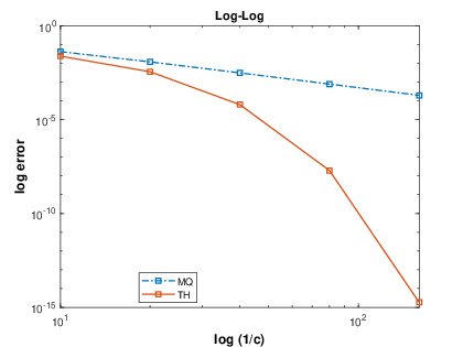
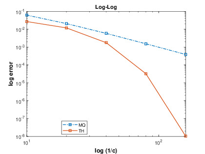
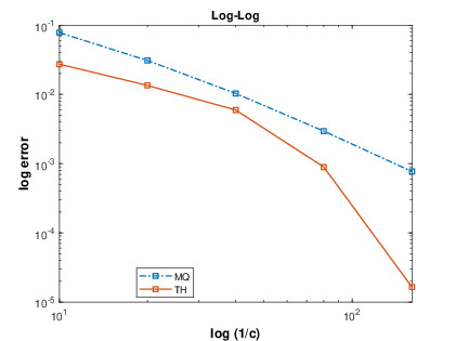
for both approximants xtanh(xc)𝑥𝑥𝑐x\tanh\left(\frac{x}{c}\right) and x2+c2superscript𝑥2superscript𝑐2\sqrt{x^{2}+c^{2}} are reported in Table 1, for n=100,200,400𝑛100200400n=100,200,400 equally spaced points in [10,10]1010[-10,10]. Table 1 shows that xtanh(xc)𝑥𝑥𝑐x\tanh\left(\frac{x}{c}\right) approximates |x|𝑥|x| much better than x2+c2superscript𝑥2superscript𝑐2\sqrt{x^{2}+c^{2}} while Table 1 and the logarithmic scale plots 1 show that the approximant xtanh(xc)𝑥𝑥𝑐x\tanh\left(\frac{x}{c}\right) has exponential rate of convergence to |x|𝑥|x| as c0𝑐0c\rightarrow 0 instead of O(c2)𝑂superscript𝑐2O(c^{2}) provided by x2+c2superscript𝑥2superscript𝑐2\sqrt{x^{2}+c^{2}}.

Table 1: Lsubscript𝐿L_{\infty} errors and convergence rates for both approximants of |x|𝑥|x| for different values of c𝑐c.
||x|x2+c2|𝑥superscript𝑥2superscript𝑐2\left|\left|x\right|-\sqrt{x^{2}+c^{2}}\right| ||x|xtanh(xc)|𝑥𝑥𝑥𝑐\left|\left|x\right|-x\tanh\left({\frac{x}{c}}\right)\right|
n𝑛n c𝑐c Lsubscript𝐿L_{\infty} error rcsubscript𝑟𝑐r_{c} Lsubscript𝐿L_{\infty} error rcsubscript𝑟𝑐r_{c}
100 0.1 4.1127e-02 2.3656e-02
0.05 1.1698e-02 1.813823944 3.4922e-03 2.759998057
0.025 3.0478e-03 1.940421754 6.2490e-05 5.804367034
0.0125 7.7050e-04 1.983901373 1.9342e-08 11.65767264
0.00625 1.9317e-04 1.995923901 1.8457e-15 23.32106557
200 0.1 6.1665e-02 2.6930e-02
0.05 2.0637e-02 1.579218611 1.1875e-02 1.181286716
0.025 5.8753e-03 1.812498837 1.7723e-03 2.744232777
0.0125 1.5314e-03 1.939811357 3.2376e-05 5.774554268
0.00625 3.8718e-04 1.983774825 1.0436e-08 11.59914019
400 0.1 7.8030e-02 2.7348e-02
0.05 3.0867e-02 1.337963627 1.3456e-02 1.023185719
0.025 1.0337e-02 1.578247724 5.9488e-03 1.177579030
0.0125 2.9442e-03 1.811869965 8.9273e-04 2.736302862
0.00625 7.6754e-04 1.939561834 1.6476e-05 5.759785971
Refer to caption
(a)
Refer to caption
(b)
Refer to caption
(c)
Figure 1: log|error|error\log|\mbox{error}| versus log(1/c)1𝑐\log\left(1/c\right) for n=100𝑛100n=100 (a), n=200𝑛200n=200 (b), and n=400𝑛400n=400 (c).

2.1 New transcendental RBF

Let us introduce the following globally supported and infinitely differentiable transcendental RBF

ϕ(r)=rtanh(rc),italic-ϕ𝑟𝑟𝑟𝑐\displaystyle\phi(r)=r\tanh\left({\frac{r}{c}}\right),

abbreviated by RTH, where r=xxj𝑟norm𝑥subscript𝑥𝑗r=\|x-x_{j}\| and \|\cdot\| is the Euclidean norm dsuperscript𝑑\mathbb{R}^{d}.

The parameter c>0𝑐0c>0 is called shape parameter whose optimal value for getting accurate numerical solutions and good conditioning of the collocation matrix, can be found usually numerically.

Theorem 2.3.

The RTH RBF is conditionally negative definite of order 111 on every dsuperscript𝑑\mathbb{R}^{d}.

Proof.

We show that ψ(r)=ϕ(r)𝜓𝑟italic-ϕ𝑟\psi(r)=-\phi(r) is conditionally positive definite of order 111. We have ψ(r)=f(s)=stanh(sc)𝜓𝑟𝑓𝑠𝑠𝑠𝑐\psi(r)=f(s)=-\sqrt{s}\tanh\left(\frac{\sqrt{s}}{c}\right), where s=r2.𝑠superscript𝑟2s=r^{2}. Now for

g(s)=f(s)=12s12tanh(sc)+12c(1tanh2(sc)),𝑔𝑠superscript𝑓𝑠12superscript𝑠12𝑠𝑐12𝑐1superscript2𝑠𝑐g(s)=-f^{\prime}(s)=\frac{1}{2}s^{-\frac{1}{2}}\tanh\left(\frac{\sqrt{s}}{c}\right)+\frac{1}{2c}\left(1-\tanh^{2}\left(\frac{\sqrt{s}}{c}\right)\right),

we have

(1)lg(l)(s)0,foralll0andalls>0.formulae-sequencesuperscript1𝑙superscript𝑔𝑙𝑠0forall𝑙subscript0andall𝑠0(-1)^{l}g^{(l)}(s)\geq 0,\quad\mbox{for}~{}\mbox{all}~{}l\in\mathbb{N}_{0}~{}\mbox{and}~{}\mbox{all}~{}s>0.

So f(s)superscript𝑓𝑠-f^{\prime}(s) is completely monotone on (0,)0(0,\infty). Now, since fΠmd𝑓superscriptsubscriptΠ𝑚𝑑f\not\in\Pi_{m}^{d} , the claim is proved according to Micchelli’s theorem [5]. ∎

Remark 2.1.

Since ϕitalic-ϕ\phi is conditionally negative definite of order 111 and ϕ(0)=0italic-ϕ00\phi(0)=0, then the matrix A=[ϕ(xixj)]1i,jn𝐴subscriptdelimited-[]italic-ϕnormsubscript𝑥𝑖subscript𝑥𝑗formulae-sequence1𝑖𝑗𝑛A=\left[\phi(\|x_{i}-x_{j}\|)\right]_{1\leq i,j\leq n} has one positive and n1𝑛1n-1 negative eigenvalues and in particular it is invertible.

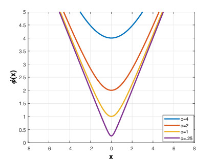
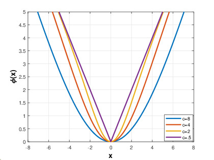
In the sequel, we consider d=1𝑑1d=1, since our work is confined to the univariate case. We have seen before that the RTH RBF is an smooth approximant to τ(r)=r𝜏𝑟𝑟\tau(r)=r with higher accuracy and better convergence properties than the MQ RBF r2+c2,superscript𝑟2superscript𝑐2\sqrt{r^{2}+c^{2}}, by decreasing shape parameter c𝑐c. In Figure 2, we have plotted both RTH basis

ϕj(x)=(xxj)tanh(xxjc),subscriptitalic-ϕ𝑗𝑥𝑥subscript𝑥𝑗𝑥subscript𝑥𝑗𝑐\displaystyle\phi_{j}(x)=\left(x-x_{j}\right)\tanh\left(\frac{x-x_{j}}{c}\right), (9)

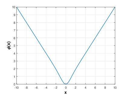
and MQ basis (2) centered at xj=0subscript𝑥𝑗0x_{j}=0. It can be noted from Figure 2 that the RTH RBF approaches to |x|𝑥|x| faster than the MQ RBF, even with larger shape parameters. Moreover, in RTH RBF ϕj(xj)=0subscriptitalic-ϕ𝑗subscript𝑥𝑗0\phi_{j}(x_{j})=0 independent of the value of c𝑐c, but MQ requires that c=0𝑐0c=0. This property of the RTH RBF leads to getting more accurate results in corresponding quasi-interpolants.
Refer to caption
Refer to caption
Figure 2: Plots of Multiquadric RBF (left), and RTH RBF (right) for different values of shape parameter c𝑐c.

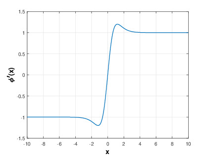
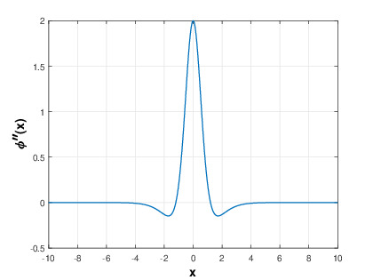
The first and second derivatives of the RTH RBF (9) are of the form

ϕj(x)subscriptsuperscriptitalic-ϕ𝑗𝑥\displaystyle\phi^{{}^{\prime}}_{j}(x) =tanh(xxjc)+(xxj)c(1(tanh(xxjc))2),absent𝑥subscript𝑥𝑗𝑐𝑥subscript𝑥𝑗𝑐1superscript𝑥subscript𝑥𝑗𝑐2\displaystyle=\tanh\left({\frac{x-x_{j}}{c}}\right)+{\frac{(x-x_{j})}{c}\left(1-\left(\tanh\left({\frac{x-x_{j}}{c}}\right)\right)^{2}\right)},
ϕj′′(x)subscriptsuperscriptitalic-ϕ′′𝑗𝑥\displaystyle\phi^{{}^{\prime\prime}}_{j}(x) =21c(1(tanh(xxjc))2)2(xxj)c2tanh(xxjc)(1(tanh(xxjc))2),absent21𝑐1superscript𝑥subscript𝑥𝑗𝑐22𝑥subscript𝑥𝑗superscript𝑐2𝑥subscript𝑥𝑗𝑐1superscript𝑥subscript𝑥𝑗𝑐2\displaystyle=2\,{\frac{1}{c}\left(1-\left(\tanh\left({\frac{x-x_{j}}{c}}\right)\right)^{2}\right)}-2\,{\frac{(x-x_{j})}{{c}^{2}}\tanh\left({\frac{x-x_{j}}{c}}\right)\left(1-\left(\tanh\left({\frac{x-x_{j}}{c}}\right)\right)^{2}\right)},

and are plotted in Figure 3 for c=1𝑐1c=1.

Refer to caption
(a)
Refer to caption
(b)
Refer to caption
(c)
Figure 3: RTH RBF (a), first derivative (b), and second derivative of RTH RBF (c) with shape parameter c=1𝑐1c=1

In Tables 2 and 3, we summarized the properties of both MQ and RTH RBFs, where ξ=1.199678640,𝜉1.199678640\xi=1.199678640, is obtained numerically by calculating the roots of the second derivative.

Table 2: Comparing both RBFs.
Name ϕj(x)subscriptitalic-ϕ𝑗𝑥\phi_{j}(x) limxxjϕj(x)subscript𝑥subscript𝑥𝑗subscriptitalic-ϕ𝑗𝑥\displaystyle\lim_{x\rightarrow x_{j}}\phi_{j}(x) limc0ϕj(x)subscript𝑐0subscriptitalic-ϕ𝑗𝑥\displaystyle\lim_{c\rightarrow 0}\phi_{j}(x) limx±ϕj(x)subscript𝑥plus-or-minussubscriptsuperscriptitalic-ϕ𝑗𝑥\displaystyle\lim_{x\rightarrow\pm\infty}\phi^{{}^{\prime}}_{j}(x) condition
MQ RBF c2+(xxj)2superscript𝑐2superscript𝑥subscript𝑥𝑗2\sqrt{c^{2}+(x-x_{j})^{2}} c𝑐c |xxj|𝑥subscript𝑥𝑗\lvert x-x_{j}\rvert ±1plus-or-minus1\pm 1 x(,)𝑥x\in(-\infty,\infty)
RTH RBF (xxj)tanh(xxjc)𝑥subscript𝑥𝑗𝑥subscript𝑥𝑗𝑐\left(x-x_{j}\right)\tanh\left(\dfrac{x-x_{j}}{c}\right) 00 |xxj|𝑥subscript𝑥𝑗\lvert x-x_{j}\rvert ±1plus-or-minus1\pm 1 x(,)𝑥x\in(-\infty,\infty)
Table 3: Comparing both RBFs.
Name ϕj(x)subscriptitalic-ϕ𝑗𝑥\phi_{j}(x) ϕj(x)subscriptsuperscriptitalic-ϕ𝑗𝑥\phi^{{}^{\prime}}_{j}(x) ϕj′′(x)subscriptsuperscriptitalic-ϕ′′𝑗𝑥\phi^{{}^{\prime\prime}}_{j}(x) condition
MQ RBF c2+(xxj)2superscript𝑐2superscript𝑥subscript𝑥𝑗2\sqrt{c^{2}+(x-x_{j})^{2}} Strictly increasing 0absent0\geq 0 x(,)𝑥x\in(-\infty,\infty)
RTH RBF (xxj)tanh(xxjc)𝑥subscript𝑥𝑗𝑥subscript𝑥𝑗𝑐\left(x-x_{j}\right)\tanh\left(\dfrac{x-x_{j}}{c}\right) Strictly increasing 0absent0\geq 0 x[cξ,cξ]𝑥𝑐𝜉𝑐𝜉x\in[-c\xi,c\xi]

2.2 Quasi-interpolation operator

The quasi-interpolation operator of a function f:[a,b]:𝑓𝑎𝑏f:[a,b]\rightarrow\mathbb{R} with RTH RBF on the scattered points

a=x0<x2<<xn=bh:=max2jn(xjxj1),formulae-sequence𝑎subscript𝑥0subscript𝑥2subscript𝑥𝑛𝑏assignsubscript2𝑗𝑛subscript𝑥𝑗subscript𝑥𝑗1\displaystyle a=x_{0}<x_{2}<\dotsb<x_{n}=b\qquad h:=\max_{2\leq j\leq n}(x_{j}-x_{j-1}), (10)

has the form

(RTHf)(x)=f0α0(x)+f1α1(x)+j=2n2fjψj(x)+fn1αn1(x)+fnαn(x)subscript𝑅𝑇𝐻𝑓𝑥subscript𝑓0subscript𝛼0𝑥subscript𝑓1subscript𝛼1𝑥superscriptsubscript𝑗2𝑛2subscript𝑓𝑗subscript𝜓𝑗𝑥subscript𝑓𝑛1subscript𝛼𝑛1𝑥subscript𝑓𝑛subscript𝛼𝑛𝑥(\mathcal{L}_{RTH}f)(x)=f_{0}\alpha_{0}(x)+f_{1}\alpha_{1}(x)+\sum_{j=2}^{n-2}f_{j}\psi_{j}(x)+f_{n-1}\alpha_{n-1}(x)+f_{n}\alpha_{n}(x) (11)

where

α0(x)subscript𝛼0𝑥\displaystyle\alpha_{0}(x) =12+ϕ1(x)(xx0)2(x1x0),absent12subscriptitalic-ϕ1𝑥𝑥subscript𝑥02subscript𝑥1subscript𝑥0\displaystyle=\dfrac{1}{2}+\dfrac{\phi_{1}(x)-(x-x_{0})}{2(x_{1}-x_{0})},
α1(x)subscript𝛼1𝑥\displaystyle\alpha_{1}(x) =ϕ2(x)ϕ1(x)2(x2x1)ϕ1(x)(xx0)2(x1x0),absentsubscriptitalic-ϕ2𝑥subscriptitalic-ϕ1𝑥2subscript𝑥2subscript𝑥1subscriptitalic-ϕ1𝑥𝑥subscript𝑥02subscript𝑥1subscript𝑥0\displaystyle=\dfrac{\phi_{2}(x)-\phi_{1}(x)}{2(x_{2}-x_{1})}-\dfrac{\phi_{1}(x)-(x-x_{0})}{2(x_{1}-x_{0})},
αn1(x)subscript𝛼𝑛1𝑥\displaystyle\alpha_{n-1}(x) =(xnx)ϕn1(x)2(xnxn1)ϕn1(x)ϕn2(x)2(xn1xn2),\displaystyle=\dfrac{(x_{n}-x)-\phi_{n-1}(x)}{2(x_{n}-x_{n-1)}}-\dfrac{\phi_{n-1}(x)-\phi_{n-2}(x)}{2(x_{n-1}-x_{n-2})},
αn(x)subscript𝛼𝑛𝑥\displaystyle\alpha_{n}(x) =12+ϕn1(x)(xnx)2(xnxn1),absent12subscriptitalic-ϕ𝑛1𝑥subscript𝑥𝑛𝑥2subscript𝑥𝑛subscript𝑥𝑛1\displaystyle=\dfrac{1}{2}+\dfrac{\phi_{n-1}(x)-(x_{n}-x)}{2(x_{n}-x_{n-1})},
ϕj(x)subscriptitalic-ϕ𝑗𝑥\displaystyle\phi_{j}(x) =(xxj)tanh(xxjc),j=1,,n1,c+,formulae-sequenceabsent𝑥subscript𝑥𝑗𝑥subscript𝑥𝑗𝑐formulae-sequence𝑗1𝑛1𝑐subscript\displaystyle=\left(x-x_{j}\right)\tanh\left(\frac{x-x_{j}}{c}\right),\quad j=1,\ldots,n-1,~{}c\in\mathbb{R}_{+},
ψj(x)subscript𝜓𝑗𝑥\displaystyle\psi_{j}(x) =ϕj+1(x)ϕj(x)2(xj+1xj)ϕj(x)ϕj1(x)2(xjxj1),2jn2.\displaystyle=\dfrac{\phi_{j+1}(x)-\phi_{j}(x)}{2(x_{j+1}-x_{j})}-\dfrac{\phi_{j}(x)-\phi_{j-1}(x)}{2(x_{j}-x_{j-1)}},\qquad 2\leq j\leq n-2.

The formula (11) can be rewritten as

(RTHf)(x)subscript𝑅𝑇𝐻𝑓𝑥\displaystyle\left(\mathcal{L}_{RTH}f\right)(x) =\displaystyle= 12j=1n1f[xj1,xj,xj+1](xj+1xj1)ϕj(x)+limit-from12superscriptsubscript𝑗1𝑛1𝑓subscript𝑥𝑗1subscript𝑥𝑗subscript𝑥𝑗1subscript𝑥𝑗1subscript𝑥𝑗1subscriptitalic-ϕ𝑗𝑥\displaystyle\frac{1}{2}\sum_{j=1}^{n-1}f[x_{j-1},x_{j},x_{j+1}](x_{j+1}-x_{j-1})\phi_{j}(x)+
f0+fn2+12f[x0,x1](xx0)12f[xn1,xn](xnx).subscript𝑓0subscript𝑓𝑛212𝑓subscript𝑥0subscript𝑥1𝑥subscript𝑥012𝑓subscript𝑥𝑛1subscript𝑥𝑛subscript𝑥𝑛𝑥\displaystyle\frac{f_{0}+f_{n}}{2}+\frac{1}{2}f[x_{0},x_{1}](x-x_{0})-\frac{1}{2}f[x_{n-1},x_{n}](x_{n}-x).

Let ϕ1(x)=|xx1|,ϕ0(x)=|xx0|,ϕn(x)=|xxn|formulae-sequencesubscriptitalic-ϕ1𝑥𝑥subscript𝑥1formulae-sequencesubscriptitalic-ϕ0𝑥𝑥subscript𝑥0subscriptitalic-ϕ𝑛𝑥𝑥subscript𝑥𝑛\phi_{-1}(x)=|x-x_{-1}|,~{}\phi_{0}(x)=|x-x_{0}|,~{}\phi_{n}(x)=|x-x_{n}| and ϕn+1(x)=|xxn+1|subscriptitalic-ϕ𝑛1𝑥𝑥subscript𝑥𝑛1\phi_{n+1}(x)=|x-x_{n+1}|, then for x[x0,xn]𝑥subscript𝑥0subscript𝑥𝑛x\in[x_{0},x_{n}], the operator RTHsubscript𝑅𝑇𝐻\mathcal{L}_{RTH} can be rearranged as

(RTHf)(x)=j=0nfjψj(x),subscript𝑅𝑇𝐻𝑓𝑥superscriptsubscript𝑗0𝑛subscript𝑓𝑗subscript𝜓𝑗𝑥\displaystyle(\mathcal{L}_{RTH}f)(x)=\sum_{j=0}^{n}f_{j}\psi_{j}(x), (13)

where

ψj(x)=ϕj+1(x)ϕj(x)2(xj+1xj)ϕj(x)ϕj1(x)2(xjxj1),j=0,,n,formulae-sequencesubscript𝜓𝑗𝑥subscriptitalic-ϕ𝑗1𝑥subscriptitalic-ϕ𝑗𝑥2subscript𝑥𝑗1subscript𝑥𝑗subscriptitalic-ϕ𝑗𝑥subscriptitalic-ϕ𝑗1𝑥2subscript𝑥𝑗subscript𝑥𝑗1𝑗0𝑛\displaystyle\psi_{j}(x)=\frac{\phi_{j+1}(x)-\phi_{j}(x)}{2(x_{j+1}-x_{j})}-\frac{\phi_{j}(x)-\phi_{j-1}(x)}{2(x_{j}-x_{j-1})},\quad j=0,\ldots,n,

and x1<x0,xn+1>xn.formulae-sequencesubscript𝑥1subscript𝑥0subscript𝑥𝑛1subscript𝑥𝑛x_{-1}<x_{0},~{}x_{n+1}>x_{n}.

Remark 2.2.

From relation (2.2), it is clear that the quasi-interpolation operator RTHsubscript𝑅𝑇𝐻\mathcal{L}_{RTH} reproduces the linear polynomials on [x0,xn]subscript𝑥0subscript𝑥𝑛[x_{0},x_{n}], that is

j=0n(axj+b)ψj(x)=ax+b,a,b,formulae-sequencesuperscriptsubscript𝑗0𝑛𝑎subscript𝑥𝑗𝑏subscript𝜓𝑗𝑥𝑎𝑥𝑏𝑎𝑏\displaystyle\sum_{j=0}^{n}(ax_{j}+b)\psi_{j}(x)=ax+b,\quad a,b\in\mathbb{R}\,, (14)

from which we also get j=0nψj(x)=1superscriptsubscript𝑗0𝑛subscript𝜓𝑗𝑥1\displaystyle\sum_{j=0}^{n}\psi_{j}(x)=1 at any point x[x0,xn]𝑥subscript𝑥0subscript𝑥𝑛x\in[x_{0},x_{n}].

In order to prove the shape-preserving property of the quasi-interpolation operator (11), we give some important definitions and theorems from differential geometry (cf. e.g. [44]).

Definition 2.1.

A differentiable plane curve α:(a,b)2:𝛼𝑎𝑏superscript2\alpha:(a,b)\rightarrow\mathbb{R}^{2} is said to be regular if its derivative never vanishes. That is

t(a,b),α(t)=(dα1dt,dα2dt)(0,0).formulae-sequencefor-all𝑡𝑎𝑏superscript𝛼𝑡𝑑subscript𝛼1𝑑𝑡𝑑subscript𝛼2𝑑𝑡00\displaystyle\forall t\in(a,b),\quad\quad\quad\quad\alpha^{\prime}(t)=\left(\frac{d\alpha_{1}}{dt},\frac{d\alpha_{2}}{dt}\right)\neq(0,0).
Theorem 2.4.

Let C𝐶C be a regular plane curve given by α(t)𝛼𝑡\alpha(t). Then the curvature κ𝜅\kappa of C𝐶C at t𝑡t is given by

κ[α](t)=α(t)×α′′(t)/α(t)3.𝜅delimited-[]𝛼𝑡normsuperscript𝛼𝑡superscript𝛼′′𝑡superscriptnormsuperscript𝛼𝑡3\kappa[\alpha](t)=\left\|\alpha^{\prime}(t)\times\alpha^{\prime\prime}(t)\right\|/\left\|\alpha^{\prime}(t)\right\|^{3}.
Definition 2.2.

Let fC2[a,b]𝑓superscript𝐶2𝑎𝑏f\in C^{2}[a,b]. The curvature of the plane curve y=f(x)𝑦𝑓𝑥y=f(x) is given by

κ(x)=|f′′(x)|(1+(f(x))2)32.𝜅𝑥superscript𝑓′′𝑥superscript1superscriptsuperscript𝑓𝑥232\kappa(x)=\dfrac{\lvert f^{\prime\prime}(x)\rvert}{(1+(f^{\prime}(x))^{2})^{\frac{3}{2}}}.
Theorem 2.5 (Fundamental theorem of plane curves).

Let α,γ:(a,b)2:𝛼𝛾𝑎𝑏superscript2\alpha,\gamma:(a,b)\rightarrow\mathbb{R}^{2} be regular plane curves such that κ[α](t)=κ[γ](t)𝜅delimited-[]𝛼𝑡𝜅delimited-[]𝛾𝑡\kappa[\alpha](t)=\kappa[\gamma](t) for all t(a,b)𝑡𝑎𝑏t\in(a,b). Then there is an orientation-preserving Euclidean motion F:22:𝐹superscript2superscript2F:\mathbb{R}^{2}\rightarrow\mathbb{R}^{2} such that γ=Foα𝛾𝐹𝑜𝛼\gamma=F~{}o~{}\alpha.

Corollary 2.5.1.

Two unit-speed plane curves which have the same curvature differ only by a Euclidean motion.

Theorem 2.6.

The quasi-interpolation operator RTHsubscript𝑅𝑇𝐻\mathcal{L}_{RTH} constructed by data points {(xj,fj)}subscript𝑥𝑗subscript𝑓𝑗\{(x_{j},f_{j})\}, is monotonicity and convexity-preserving for c𝑐c small enough.

Proof.

According to the Corollary 2.5.1, it suffices to show that

limc0|κMQ(x)κRTH(x)|=0.subscript𝑐0subscript𝜅subscript𝑀𝑄𝑥subscript𝜅subscript𝑅𝑇𝐻𝑥0\displaystyle\displaystyle\lim_{c\rightarrow 0}\lvert\kappa_{\mathcal{L}_{MQ}}(x)-\kappa_{\mathcal{L}_{RTH}}(x)\rvert=0.

Let xxj𝑥subscript𝑥𝑗x\neq x_{j}, otherwise both quasi-interpolants (3) and (11) do not have first and second derivatives as c𝑐c approaches 00. Now, according to definition 2.2, we have

κMQ(x)=|(MQf)′′(x)|(1+((MQf)(x))2)32.subscript𝜅subscript𝑀𝑄𝑥superscriptsubscript𝑀𝑄𝑓′′𝑥superscript1superscriptsuperscriptsubscript𝑀𝑄𝑓𝑥232\displaystyle\kappa_{{\mathcal{L}_{MQ}}}(x)=\dfrac{\lvert({\mathcal{L}_{MQ}}f)^{\prime\prime}(x)\rvert}{\left(1+\left(({\mathcal{L}_{MQ}}f)^{\prime}(x)\right)^{2}\right)^{\frac{3}{2}}}.

Since for MQ RBF,

ϕj′′(x)=c2(c2+(xxj)2)3/2,superscriptsubscriptitalic-ϕ𝑗′′𝑥superscript𝑐2superscriptsuperscript𝑐2superscript𝑥subscript𝑥𝑗232\displaystyle\phi_{j}^{\prime\prime}(x)=\frac{c^{2}}{\left(c^{2}+(x-x_{j})^{2}\right)^{3/2}},

then

limc0ϕj′′(x)=0.subscript𝑐0superscriptsubscriptitalic-ϕ𝑗′′𝑥0\displaystyle\lim_{c\longrightarrow 0}\phi_{j}^{\prime\prime}(x)=0.

Moreover

(MQf)′′(x)=12j=1n1[fj+1fjxj+1xjfjfj1xjxj1]ϕj′′(x),superscriptsubscript𝑀𝑄𝑓′′𝑥12superscriptsubscript𝑗1𝑛1delimited-[]subscript𝑓𝑗1subscript𝑓𝑗subscript𝑥𝑗1subscript𝑥𝑗subscript𝑓𝑗subscript𝑓𝑗1subscript𝑥𝑗subscript𝑥𝑗1superscriptsubscriptitalic-ϕ𝑗′′𝑥\displaystyle(\mathcal{L}_{MQ}f)^{\prime\prime}(x)=\dfrac{1}{2}\sum_{j=1}^{n-1}\left[\dfrac{f_{j+1}-f_{j}}{x_{j+1}-x_{j}}-\dfrac{f_{j}-f_{j-1}}{x_{j}-x_{j-1}}\right]\phi_{j}^{\prime\prime}(x),

then

limc0κMQ(x)=0,subscript𝑐0subscript𝜅subscript𝑀𝑄𝑥0\displaystyle\lim_{c\longrightarrow 0}\kappa_{\mathcal{L}_{{{MQ}}}}(x)=0,

which leads to

ϵ>0δ1>0;|c|<δ1|κMQ(x)|<ϵ.formulae-sequencefor-allitalic-ϵ0formulae-sequencesubscript𝛿10𝑐subscript𝛿1subscript𝜅subscript𝑀𝑄𝑥italic-ϵ\displaystyle\forall\epsilon>0\quad\exists\delta_{1}>0;\quad\lvert\,c\,\rvert<\delta_{1}\Rightarrow\lvert\kappa_{\mathcal{L}_{{{MQ}}}}(x)\rvert<\epsilon.

Similarly, for RTH RBF, we have

limc0ϕj′′(x)=0,subscript𝑐0superscriptsubscriptitalic-ϕ𝑗′′𝑥0\displaystyle\lim_{c\longrightarrow 0}\phi_{j}^{\prime\prime}(x)=0,

then

limc0κRTH(x)=0,subscript𝑐0subscript𝜅subscript𝑅𝑇𝐻𝑥0\displaystyle\lim_{c\longrightarrow 0}\kappa_{\mathcal{L}_{{{RTH}}}}(x)=0,

which leads to

ϵ>0δ2>0;|c|<δ2|κRTH(x)|<ϵ.formulae-sequencefor-allitalic-ϵ0formulae-sequencesubscript𝛿20𝑐subscript𝛿2subscript𝜅subscript𝑅𝑇𝐻𝑥italic-ϵ\displaystyle\forall\epsilon>0\quad\exists\delta_{2}>0;\quad\lvert\,c\,\rvert<\delta_{2}\Rightarrow\lvert\kappa_{\mathcal{L}_{{{RTH}}}}(x)\rvert<\epsilon.

The proof completes by considering δ=min{δ1,δ2}𝛿subscript𝛿1subscript𝛿2\delta=\min\{\delta_{1},\delta_{2}\}. ∎

3 Accuracy of the quasi-interpolation operator RTHsubscript𝑅𝑇𝐻\mathcal{L}_{RTH}

In this section, we give an approximation order for the quasi-interpolation operator RTH.subscript𝑅𝑇𝐻\mathcal{L}_{RTH}.

Theorem 3.1.

Assume f′′superscript𝑓′′f^{\prime\prime} is Lipschitz continuous. The quasi-interpolation operator RTHfsubscript𝑅𝑇𝐻𝑓\mathcal{L}_{RTH}f, at the point set (10) as h00h\rightarrow 0, converges as follows

fRTHfkh2,subscriptnorm𝑓subscript𝑅𝑇𝐻𝑓𝑘superscript2\displaystyle\|f-\mathcal{L}_{RTH}f\|_{\infty}\leq kh^{2}, (15)

where k𝑘k is independent of hh and c𝑐c.

Proof.

Let t(y)𝑡𝑦t(y) be the local Taylor approximation of f𝑓f at y𝑦y, that is

t(y)=f(x)+f(x)(yx),x[a,b]formulae-sequence𝑡𝑦𝑓𝑥superscript𝑓𝑥𝑦𝑥𝑥𝑎𝑏\displaystyle t(y)=f(x)+f^{\prime}(x)(y-x)\,,\;\;x\in[a,b]

According to Remark 2.2, we get

j=0n(xxj)ψj(x)=0,j=0nψj(x)=1.formulae-sequencesuperscriptsubscript𝑗0𝑛𝑥subscript𝑥𝑗subscript𝜓𝑗𝑥0superscriptsubscript𝑗0𝑛subscript𝜓𝑗𝑥1\displaystyle\sum_{j=0}^{n}(x-x_{j})\psi_{j}(x)=0,\quad\sum_{j=0}^{n}\psi_{j}(x)=1.

Then we get

j=0nt(xj)ψj(x)superscriptsubscript𝑗0𝑛𝑡subscript𝑥𝑗subscript𝜓𝑗𝑥\displaystyle\sum_{j=0}^{n}t(x_{j})\psi_{j}(x) =\displaystyle= j=0n[f(x)+f(x)(xjx)]ψj(x)superscriptsubscript𝑗0𝑛delimited-[]𝑓𝑥superscript𝑓𝑥subscript𝑥𝑗𝑥subscript𝜓𝑗𝑥\displaystyle\sum_{j=0}^{n}\left[f(x)+f^{\prime}(x)(x_{j}-x)\right]\psi_{j}(x)
=\displaystyle= f(x)j=0nψj(x)+f(x)j=0n(xxj)ψj(x)𝑓𝑥superscriptsubscript𝑗0𝑛subscript𝜓𝑗𝑥superscript𝑓𝑥superscriptsubscript𝑗0𝑛𝑥subscript𝑥𝑗subscript𝜓𝑗𝑥\displaystyle f(x)\sum_{j=0}^{n}\psi_{j}(x)+f^{\prime}(x)\sum_{j=0}^{n}(x-x_{j})\psi_{j}(x)
=\displaystyle= f(x).𝑓𝑥\displaystyle f(x).

Since f′′(x)superscript𝑓′′𝑥f^{\prime\prime}(x) is Lipschitz continuous, then for every x1,x2[a,b]subscript𝑥1subscript𝑥2𝑎𝑏x_{1},~{}x_{2}\in[a,b], |f′′(x1)f′′(x2)|c0|x1x2|,superscript𝑓′′subscript𝑥1superscript𝑓′′subscript𝑥2subscript𝑐0subscript𝑥1subscript𝑥2|f^{\prime\prime}(x_{1})-f^{\prime\prime}(x_{2})|\leq c_{0}|x_{1}-x_{2}|, where 0<c0=ess supaxb|f′′′(x)|0subscript𝑐0subscriptess sup𝑎𝑥𝑏superscript𝑓′′′𝑥\displaystyle 0<c_{0}=\mbox{ess sup}_{a\leq x\leq b}|f^{\prime\prime\prime}(x)|. Now according to (2.2), we have

|RTHf(x)f(x)|subscript𝑅𝑇𝐻𝑓𝑥𝑓𝑥\displaystyle|\mathcal{L}_{RTH}f(x)-f(x)| =\displaystyle= |j=0n(f(xj)t(xj))ψj(x)|superscriptsubscript𝑗0𝑛𝑓subscript𝑥𝑗𝑡subscript𝑥𝑗subscript𝜓𝑗𝑥\displaystyle\left|\sum_{j=0}^{n}\left(f(x_{j})-t(x_{j})\right)\psi_{j}(x)\right|
\displaystyle\leq 12|j=1n1(f[xj1,xj,xj+1]t[xj1,xj,xj+1])(xj+1xj1)ϕj(x)|12superscriptsubscript𝑗1𝑛1𝑓subscript𝑥𝑗1subscript𝑥𝑗subscript𝑥𝑗1𝑡subscript𝑥𝑗1subscript𝑥𝑗subscript𝑥𝑗1subscript𝑥𝑗1subscript𝑥𝑗1subscriptitalic-ϕ𝑗𝑥\displaystyle\frac{1}{2}\left|\sum_{j=1}^{n-1}\left(f[x_{j-1},x_{j},x_{j+1}]-t[x_{j-1},x_{j},x_{j+1}]\right)(x_{j+1}-x_{j-1})\phi_{j}(x)\right|
+c1(xx0)2+c2(xnx)2subscript𝑐1superscript𝑥subscript𝑥02subscript𝑐2superscriptsubscript𝑥𝑛𝑥2\displaystyle+c_{1}(x-x_{0})^{2}+c_{2}(x_{n}-x)^{2}
\displaystyle\leq 14j=1n1|f′′(ξ)f′′(η)||ϕj(x)(xj+1xj1)|,(ξ,η(xj1,xj+1))14superscriptsubscript𝑗1𝑛1superscript𝑓′′𝜉superscript𝑓′′𝜂subscriptitalic-ϕ𝑗𝑥subscript𝑥𝑗1subscript𝑥𝑗1𝜉𝜂subscript𝑥𝑗1subscript𝑥𝑗1\displaystyle\frac{1}{4}\sum_{j=1}^{n-1}|f^{\prime\prime}(\xi)-f^{\prime\prime}(\eta)||\phi_{j}(x)\,(x_{j+1}-x_{j-1})|,\quad(\xi,\eta\in(x_{j-1},x_{j+1}))
+c1(xx0)2+c2(xnx)2subscript𝑐1superscript𝑥subscript𝑥02subscript𝑐2superscriptsubscript𝑥𝑛𝑥2\displaystyle+c_{1}(x-x_{0})^{2}+c_{2}(x_{n}-x)^{2}
\displaystyle\leq 12c0hj=1n1|xxj|(xj+1xj1)+c1(xx0)2+c2(xnx)212subscript𝑐0superscriptsubscript𝑗1𝑛1𝑥subscript𝑥𝑗subscript𝑥𝑗1subscript𝑥𝑗1subscript𝑐1superscript𝑥subscript𝑥02subscript𝑐2superscriptsubscript𝑥𝑛𝑥2\displaystyle\frac{1}{2}c_{0}h\sum_{j=1}^{n-1}|x-x_{j}|(x_{j+1}-x_{j-1})+c_{1}(x-x_{0})^{2}+c_{2}(x_{n}-x)^{2}
\displaystyle\leq 12c0hj=1|xxj|hn1|xxj|(xj+1xj1)+12c0hj=1|xxj|>hn1|xxj|(xj+1xj1)12subscript𝑐0superscriptsubscriptsubscript𝑗1𝑥subscript𝑥𝑗𝑛1𝑥subscript𝑥𝑗subscript𝑥𝑗1subscript𝑥𝑗112subscript𝑐0superscriptsubscriptsubscript𝑗1𝑥subscript𝑥𝑗𝑛1𝑥subscript𝑥𝑗subscript𝑥𝑗1subscript𝑥𝑗1\displaystyle\frac{1}{2}c_{0}h\sum_{\displaystyle\mathop{j=1}_{|x-x_{j}|\leq h}}^{n-1}|x-x_{j}|(x_{j+1}-x_{j-1})+\frac{1}{2}c_{0}h\sum_{\displaystyle\mathop{j=1}_{|x-x_{j}|>h}}^{n-1}|x-x_{j}|(x_{j+1}-x_{j-1})
+c1(xx0)2+c2(xnx)2subscript𝑐1superscript𝑥subscript𝑥02subscript𝑐2superscriptsubscript𝑥𝑛𝑥2\displaystyle+c_{1}(x-x_{0})^{2}+c_{2}(x_{n}-x)^{2}
\displaystyle\leq 4c0h3+c0h(|xt|>h|xt|𝑑t+O(h))+c1(xx0)2+c2(xnx)24subscript𝑐0superscript3subscript𝑐0subscript𝑥𝑡𝑥𝑡differential-d𝑡𝑂subscript𝑐1superscript𝑥subscript𝑥02subscript𝑐2superscriptsubscript𝑥𝑛𝑥2\displaystyle 4c_{0}h^{3}+c_{0}h\left(\int_{|x-t|>h}|x-t|~{}dt+O(h)\right)+c_{1}(x-x_{0})^{2}+c_{2}(x_{n}-x)^{2}
\displaystyle\leq k1h3+k2h2+k3(ba)2subscript𝑘1superscript3subscript𝑘2superscript2subscript𝑘3superscript𝑏𝑎2\displaystyle k_{1}h^{3}+k_{2}h^{2}+k_{3}{(b-a)}^{2}
\displaystyle\leq kh2𝑘superscript2\displaystyle kh^{2}

4 Numerical results

In this section, we compare the accuracy of the quasi-interpolation operator RTHsubscript𝑅𝑇𝐻\mathcal{L}_{RTH} with that of Wu and Schaback, MQsubscript𝑀𝑄\mathcal{L}_{MQ} (defined in (3)) for the approximation of five functions. We take equidistant center points and choose different shape parameters c𝑐c and also different step sizes hh. The maximum absolute error norm is then computed for comparing approximation accuracy. The rate of convergence is also computed by

rh=ln(EhiEhi1)ln(hihi1),subscript𝑟subscript𝐸subscript𝑖subscript𝐸subscript𝑖1subscript𝑖subscript𝑖1r_{h}=\frac{\ln\left(\frac{E_{h_{i}}}{E_{h_{i-1}}}\right)}{\ln\left(\frac{h_{i}}{h_{i-1}}\right)},

where Ehisubscript𝐸subscript𝑖E_{h_{i}} indicates the error of the quasi-interpolant RTHfsubscript𝑅𝑇𝐻𝑓\mathcal{L}_{RTH}f corresponding to the parameter hisubscript𝑖h_{i}. In all tests, we chose m=200𝑚200m=200 equidistant evaluation points.

4.1 Test problem 1

In the first test problem, we apply the RTH quasi-interpolation to approximate the function (cf. [45])

f1(x)=sinh(x)1+cosh(x),x[3,3].formulae-sequencesubscript𝑓1𝑥𝑥1𝑥𝑥33\displaystyle f_{1}(x)=\frac{\sinh(x)}{1+\cosh(x)},\quad x\in[-3,3].

The results are shown in Tables 4-6. In Tables 4, 5, and 6, we set h=0.1,0.01,0.0010.10.010.001h=0.1,0.01,0.001, respectively, and c=2h,h,0.5h,0.2h,0.1h𝑐20.50.20.1c=2h,h,0.5h,0.2h,0.1h, then we compute the RTHffsubscriptnormsubscript𝑅𝑇𝐻𝑓𝑓\|\mathcal{L}_{RTH}f-f\|_{\infty} and MQffsubscriptnormsubscript𝑀𝑄𝑓𝑓\|\mathcal{L}_{MQ}f-f\|_{\infty}. In Table 7, we set c=0.01𝑐0.01c=0.01, h=0.2,0.1,0.05,0.025,0.01250.20.10.050.0250.0125h=0.2,0.1,0.05,0.025,0.0125, to observe the convergence rate rhsubscript𝑟r_{h} of RTHfsubscript𝑅𝑇𝐻𝑓\mathcal{L}_{RTH}f with the variation of hh.

Table 4: Comparison of approximation accuracy of RTH and MQ quasi-interpolation for the test problem 1.
c𝑐c 0.20.20.2 0.10.10.1 0.050.050.05 0.020.020.02 0.010.010.01
hh 0.10.10.1 0.10.10.1 0.10.10.1 0.10.10.1 0.10.10.1
MQffsubscriptnormsubscript𝑀𝑄𝑓𝑓\|\mathcal{L}_{MQ}f-f\|_{\infty} 9.3×1039.3superscript1039.3\times 10^{-3} 3.1×1033.1superscript1033.1\times 10^{-3} 1.1×1031.1superscript1031.1\times 10^{-3} 3.8×1043.8superscript1043.8\times 10^{-4} 2.8×1042.8superscript1042.8\times 10^{-4}
RTHffsubscriptnormsubscript𝑅𝑇𝐻𝑓𝑓\|\mathcal{L}_{RTH}f-f\|_{\infty} 2.9×1032.9superscript1032.9\times 10^{-3} 6.2×1046.2superscript1046.2\times 10^{-4} 7.1×1057.1superscript1057.1\times 10^{-5} 2.3×1042.3superscript1042.3\times 10^{-4} 2.4×1042.4superscript1042.4\times 10^{-4}
Table 5: Comparison of approximation accuracy of RTH and MQ quasi-interpolation for the test problem 1.
c𝑐c 0.020.020.02 0.010.010.01 0.0050.0050.005 0.0020.0020.002 0.0010.0010.001
hh 0.010.010.01 0.010.010.01 0.010.010.01 0.010.010.01 0.010.010.01
MQffsubscriptnormsubscript𝑀𝑄𝑓𝑓\|\mathcal{L}_{MQ}f-f\|_{\infty} 1.8×1041.8superscript1041.8\times 10^{-4} 5.3×1055.3superscript1055.3\times 10^{-5} 1.6×1051.6superscript1051.6\times 10^{-5} 3.7×1063.7superscript1063.7\times 10^{-6} 1.4×1061.4superscript1061.4\times 10^{-6}
RTHffsubscriptnormsubscript𝑅𝑇𝐻𝑓𝑓\|\mathcal{L}_{RTH}f-f\|_{\infty} 3.0×1053.0superscript1053.0\times 10^{-5} 6.3×1066.3superscript1066.3\times 10^{-6} 7.2×1077.2superscript1077.2\times 10^{-7} 1.7×1091.7superscript1091.7\times 10^{-9} 7.9×10147.9superscript10147.9\times 10^{-14}
Table 6: Comparison of approximation accuracy of RTH and MQ quasi-interpolation for the test problem 1.
c𝑐c 0.0020.0020.002 0.0010.0010.001 0.00050.00050.0005 0.00020.00020.0002 0.00010.00010.0001
hh 0.0010.0010.001 0.0010.0010.001 0.0010.0010.001 0.0010.0010.001 0.0010.0010.001
MQffsubscriptnormsubscript𝑀𝑄𝑓𝑓\|\mathcal{L}_{MQ}f-f\|_{\infty} 2.7×1062.7superscript1062.7\times 10^{-6} 7.5×1077.5superscript1077.5\times 10^{-7} 2.1×1072.1superscript1072.1\times 10^{-7} 4.6×1084.6superscript1084.6\times 10^{-8} 1.6×1081.6superscript1081.6\times 10^{-8}
RTHffsubscriptnormsubscript𝑅𝑇𝐻𝑓𝑓\|\mathcal{L}_{RTH}f-f\|_{\infty} 3.0×1073.0superscript1073.0\times 10^{-7} 6.3×1086.3superscript1086.3\times 10^{-8} 7.2×1097.2superscript1097.2\times 10^{-9} 1.7×10111.7superscript10111.7\times 10^{-11} 1.1×10151.1superscript10151.1\times 10^{-15}
Table 7: Convergence rates of RTHfsubscript𝑅𝑇𝐻𝑓\mathcal{L}_{RTH}f by using c=0.01𝑐0.01c=0.01, h=0.2,0.1,0.05,0.025,0.01250.20.10.050.0250.0125h=0.2,0.1,0.05,0.025,0.0125 for the test problem 1.
c𝑐c 0.010.010.01 0.010.010.01 0.010.010.01 0.010.010.01 0.010.010.01
hh 0.20.20.2 0.10.10.1 0.050.050.05 0.0250.0250.025 0.01250.01250.0125
RTHffsubscriptnormsubscript𝑅𝑇𝐻𝑓𝑓\|\mathcal{L}_{RTH}f-f\|_{\infty} 9.5×1049.5superscript1049.5\times 10^{-4} 2.4×1042.4superscript1042.4\times 10^{-4} 5.4×1055.4superscript1055.4\times 10^{-5} 5.1×1065.1superscript1065.1\times 10^{-6} 1.0×1061.0superscript1061.0\times 10^{-6}
rhsubscript𝑟r_{h} - 1.98551.98551.9855 2.16572.16572.1657 3.40563.40563.4056 2.30282.30282.3028

4.2 Test problem 2

In this experiment we apply the RTH quasi-interpolation to approximate the function (again considered in [45])

f2(x)=sin(x2)2cos(x)+4sin(πx),x[4,4].formulae-sequencesubscript𝑓2𝑥𝑥22𝑥4𝜋𝑥𝑥44\displaystyle f_{2}(x)=\sin\left(\frac{x}{2}\right)-2\cos(x)+4\sin(\pi x),\quad x\in[-4,4]. (16)

The comparison results are shown in Tables 8-10. In Tables 8, 9, and 10, we set h=0.1,0.01,0.0010.10.010.001h=0.1,0.01,0.001, respectively, and c=2h,h,0.5h,0.2h,0.1h𝑐20.50.20.1c=2h,h,0.5h,0.2h,0.1h, then we compute the RTHffsubscriptnormsubscript𝑅𝑇𝐻𝑓𝑓\|\mathcal{L}_{RTH}f-f\|_{\infty} and MQffsubscriptnormsubscript𝑀𝑄𝑓𝑓\|\mathcal{L}_{MQ}f-f\|_{\infty}. In Table 11, we set c=0.01𝑐0.01c=0.01, h=0.2,0.1,0.05,0.025,0.01250.20.10.050.0250.0125h=0.2,0.1,0.05,0.025,0.0125, to observe the convergence rate rhsubscript𝑟r_{h} of RTHfsubscript𝑅𝑇𝐻𝑓\mathcal{L}_{RTH}f with the variation of hh.

Table 8: Comparison of approximation accuracy of RTH and MQ quasi-interpolation for the test problem 2.
c𝑐c 0.20.20.2 0.10.10.1 0.050.050.05 0.020.020.02 0.010.010.01
hh 0.10.10.1 0.10.10.1 0.10.10.1 0.10.10.1 0.10.10.1
MQffsubscriptnormsubscript𝑀𝑄𝑓𝑓\|\mathcal{L}_{MQ}f-f\|_{\infty} 1.21.21.2 4.5×1014.5superscript1014.5\times 10^{-1} 1.7×1011.7superscript1011.7\times 10^{-1} 7.1×1027.1superscript1027.1\times 10^{-2} 5.4×1025.4superscript1025.4\times 10^{-2}
RTHffsubscriptnormsubscript𝑅𝑇𝐻𝑓𝑓\|\mathcal{L}_{RTH}f-f\|_{\infty} 4.5×1014.5superscript1014.5\times 10^{-1} 1.2×1011.2superscript1011.2\times 10^{-1} 1.4×1021.4superscript1021.4\times 10^{-2} 4.5×1024.5superscript1024.5\times 10^{-2} 4.9×1024.9superscript1024.9\times 10^{-2}
Table 9: Comparison of approximation accuracy of RTH and MQ quasi-interpolation for the test problem 2.
c𝑐c 0.020.020.02 0.010.010.01 0.0050.0050.005 0.0020.0020.002 0.0010.0010.001
hh 0.010.010.01 0.010.010.01 0.010.010.01 0.010.010.01 0.010.010.01
MQffsubscriptnormsubscript𝑀𝑄𝑓𝑓\|\mathcal{L}_{MQ}f-f\|_{\infty} 3.0×1023.0superscript1023.0\times 10^{-2} 9.2×1039.2superscript1039.2\times 10^{-3} 2.9×1032.9superscript1032.9\times 10^{-3} 7.1×1047.1superscript1047.1\times 10^{-4} 2.8×1042.8superscript1042.8\times 10^{-4}
RTHffsubscriptnormsubscript𝑅𝑇𝐻𝑓𝑓\|\mathcal{L}_{RTH}f-f\|_{\infty} 6.4×1036.4superscript1036.4\times 10^{-3} 1.4×1031.4superscript1031.4\times 10^{-3} 1.5×1041.5superscript1041.5\times 10^{-4} 3.7×1073.7superscript1073.7\times 10^{-7} 1.7×10111.7superscript10111.7\times 10^{-11}
Table 10: Comparison of approximation accuracy of RTH and MQ quasi-interpolation for the test problem 2.
c𝑐c 0.0020.0020.002 0.0010.0010.001 0.00050.00050.0005 0.00020.00020.0002 0.00010.00010.0001
hh 0.0010.0010.001 0.0010.0010.001 0.0010.0010.001 0.0010.0010.001 0.0010.0010.001
MQffsubscriptnormsubscript𝑀𝑄𝑓𝑓\|\mathcal{L}_{MQ}f-f\|_{\infty} 4.9×1044.9superscript1044.9\times 10^{-4} 1.4×1041.4superscript1041.4\times 10^{-4} 4.1×1054.1superscript1054.1\times 10^{-5} 9.0×1069.0superscript1069.0\times 10^{-6} 3.3×1063.3superscript1063.3\times 10^{-6}
RTHffsubscriptnormsubscript𝑅𝑇𝐻𝑓𝑓\|\mathcal{L}_{RTH}f-f\|_{\infty} 6.4×1056.4superscript1056.4\times 10^{-5} 1.4×1051.4superscript1051.4\times 10^{-5} 1.5×1061.5superscript1061.5\times 10^{-6} 3.7×1093.7superscript1093.7\times 10^{-9} 1.7×10131.7superscript10131.7\times 10^{-13}
Table 11: Convergence rates of RTHfsubscript𝑅𝑇𝐻𝑓\mathcal{L}_{RTH}f by using c=0.01𝑐0.01c=0.01, h=0.2,0.1,0.05,0.025,0.01250.20.10.050.0250.0125h=0.2,0.1,0.05,0.025,0.0125 for the test problem 2.
c𝑐c 0.010.010.01 0.010.010.01 0.010.010.01 0.010.010.01 0.010.010.01
hh 0.20.20.2 0.10.10.1 0.050.050.05 0.0250.0250.025 0.01250.01250.0125
RTHffsubscriptnormsubscript𝑅𝑇𝐻𝑓𝑓\|\mathcal{L}_{RTH}f-f\|_{\infty} 2.0×1012.0superscript1012.0\times 10^{-1} 4.9×1024.9superscript1024.9\times 10^{-2} 1.1×1021.1superscript1021.1\times 10^{-2} 1.1×1031.1superscript1031.1\times 10^{-3} 2.7×1042.7superscript1042.7\times 10^{-4}
rhsubscript𝑟r_{h} - 2.01012.01012.0101 2.08992.08992.0899 3.42623.42623.4262 2.00342.00342.0034

4.3 Test problem 3

Consider the function (see again [45])

f3(x)=10ex2+x2,x[3,3],formulae-sequencesubscript𝑓3𝑥10superscript𝑒superscript𝑥2superscript𝑥2𝑥33\displaystyle f_{3}(x)=10e^{-x^{2}}+x^{2},\quad x\in[-3,3], (17)

for approximating by the RTH quasi-interpolation operator. The comparison results are shown in Tables 12-14. In Tables 12, 13, and 14, we set h=0.1,0.01,0.0010.10.010.001h=0.1,0.01,0.001, respectively, and c=2h,h,0.5h,0.2h,0.1h𝑐20.50.20.1c=2h,h,0.5h,0.2h,0.1h, then we compute the RTHffsubscriptnormsubscript𝑅𝑇𝐻𝑓𝑓\|\mathcal{L}_{RTH}f-f\|_{\infty} and MQffsubscriptnormsubscript𝑀𝑄𝑓𝑓\|\mathcal{L}_{MQ}f-f\|_{\infty}. In Table 15, we set c=0.01𝑐0.01c=0.01, h=0.2,0.1,0.05,0.025,0.01250.20.10.050.0250.0125h=0.2,0.1,0.05,0.025,0.0125, to observe the convergence rate rhsubscript𝑟r_{h} of RTHfsubscript𝑅𝑇𝐻𝑓\mathcal{L}_{RTH}f on varying hh.

Table 12: Comparison of approximation accuracy of RTH and MQ quasi-interpolation for the test problem 3.
c𝑐c 0.20.20.2 0.10.10.1 0.050.050.05 0.020.020.02 0.010.010.01
hh 0.10.10.1 0.10.10.1 0.10.10.1 0.10.10.1 0.10.10.1
MQffsubscriptnormsubscript𝑀𝑄𝑓𝑓\|\mathcal{L}_{MQ}f-f\|_{\infty} 4.9×1014.9superscript1014.9\times 10^{-1} 2.0×1012.0superscript1012.0\times 10^{-1} 7.4×1027.4superscript1027.4\times 10^{-2} 3.1×1023.1superscript1023.1\times 10^{-2} 2.4×1022.4superscript1022.4\times 10^{-2}
RTHffsubscriptnormsubscript𝑅𝑇𝐻𝑓𝑓\|\mathcal{L}_{RTH}f-f\|_{\infty} 2.2×1012.2superscript1012.2\times 10^{-1} 5.5×1025.5superscript1025.5\times 10^{-2} 6.4×1036.4superscript1036.4\times 10^{-3} 2.0×1022.0superscript1022.0\times 10^{-2} 2.1×1022.1superscript1022.1\times 10^{-2}
Table 13: Comparison of approximation accuracy of RTH and MQ quasi-interpolation for the test problem 3.
c𝑐c 0.020.020.02 0.010.010.01 0.0050.0050.005 0.0020.0020.002 0.0010.0010.001
hh 0.010.010.01 0.010.010.01 0.010.010.01 0.010.010.01 0.010.010.01
MQffsubscriptnormsubscript𝑀𝑄𝑓𝑓\|\mathcal{L}_{MQ}f-f\|_{\infty} 1.3×1021.3superscript1021.3\times 10^{-2} 4.0×1034.0superscript1034.0\times 10^{-3} 1.3×1031.3superscript1031.3\times 10^{-3} 3.1×1043.1superscript1043.1\times 10^{-4} 1.2×1041.2superscript1041.2\times 10^{-4}
RTHffsubscriptnormsubscript𝑅𝑇𝐻𝑓𝑓\|\mathcal{L}_{RTH}f-f\|_{\infty} 2.8×1032.8superscript1032.8\times 10^{-3} 5.9×1045.9superscript1045.9\times 10^{-4} 6.7×1056.7superscript1056.7\times 10^{-5} 1.6×1071.6superscript1071.6\times 10^{-7} 7.4×10127.4superscript10127.4\times 10^{-12}
Table 14: Comparison of approximation accuracy of RTH and MQ quasi-interpolation for the test problem 3.
c𝑐c 0.0020.0020.002 0.0010.0010.001 0.00050.00050.0005 0.00020.00020.0002 0.00010.00010.0001
hh 0.0010.0010.001 0.0010.0010.001 0.0010.0010.001 0.0010.0010.001 0.0010.0010.001
MQffsubscriptnormsubscript𝑀𝑄𝑓𝑓\|\mathcal{L}_{MQ}f-f\|_{\infty} 2.1×1042.1superscript1042.1\times 10^{-4} 6.0×1056.0superscript1056.0\times 10^{-5} 1.8×1051.8superscript1051.8\times 10^{-5} 3.9×1063.9superscript1063.9\times 10^{-6} 1.4×1061.4superscript1061.4\times 10^{-6}
RTHffsubscriptnormsubscript𝑅𝑇𝐻𝑓𝑓\|\mathcal{L}_{RTH}f-f\|_{\infty} 2.8×1052.8superscript1052.8\times 10^{-5} 5.9×1065.9superscript1065.9\times 10^{-6} 6.7×1076.7superscript1076.7\times 10^{-7} 1.6×1091.6superscript1091.6\times 10^{-9} 7.5×10147.5superscript10147.5\times 10^{-14}
Table 15: Convergence rates of RTHfsubscript𝑅𝑇𝐻𝑓\mathcal{L}_{RTH}f by using c=0.01𝑐0.01c=0.01, h=0.2,0.1,0.05,0.025,0.01250.20.10.050.0250.0125h=0.2,0.1,0.05,0.025,0.0125; Test Problem 3.
c𝑐c 0.010.010.01 0.010.010.01 0.010.010.01 0.010.010.01 0.010.010.01
hh 0.20.20.2 0.10.10.1 0.050.050.05 0.0250.0250.025 0.01250.01250.0125
RTHffsubscriptnormsubscript𝑅𝑇𝐻𝑓𝑓\|\mathcal{L}_{RTH}f-f\|_{\infty} 8.6×1028.6superscript1028.6\times 10^{-2} 2.1×1022.1superscript1022.1\times 10^{-2} 5.0×1035.0superscript1035.0\times 10^{-3} 4.7×1044.7superscript1044.7\times 10^{-4} 2.6×1042.6superscript1042.6\times 10^{-4}
rhsubscript𝑟r_{h} - 2.00852.00852.0085 2.09432.09432.0943 3.42103.42103.4210 2.04192.04192.0419
Remark 4.1.

By analyzing the results in Tables 4-6, 8-10, and 12-14, we see that the accuracy of the RTH quasi-interpolation scheme is dependent on the shape parameter c𝑐c and on step size hh. Furthermore, the accuracy of the RTH quasi-interpolation operator is better than that of MQ for the same values of c𝑐c and hh. From Tables 7, 11, 15, we see that the convergence rate of RTHsubscript𝑅𝑇𝐻\mathcal{L}_{RTH} reaches up to 222 which justifies our theoretical findings of Section 3. By these numerical experiments, we can say that the quasi-interpolation RTHsubscript𝑅𝑇𝐻\mathcal{L}_{RTH} is a very attractive alternative, in terms of accuracy and convergence, to MQsubscript𝑀𝑄\mathcal{L}_{MQ}.

4.4 Test problem 4 (Runge function)

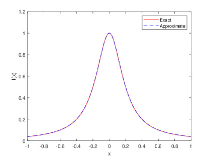
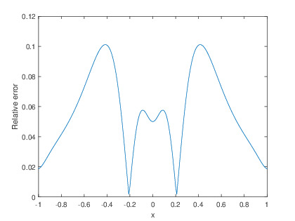
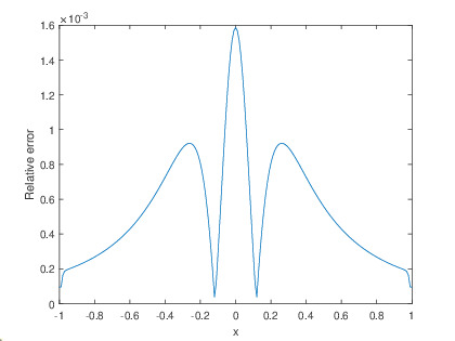
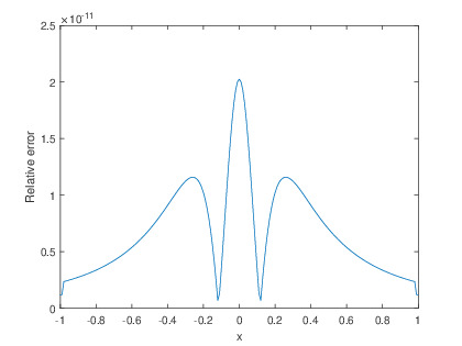
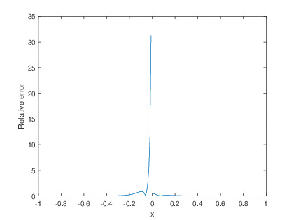
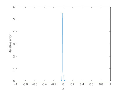
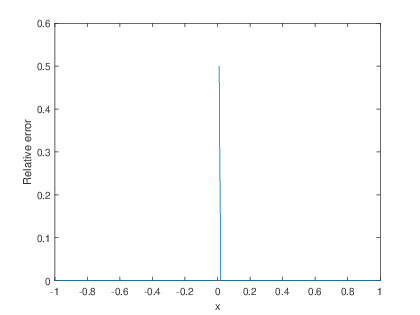
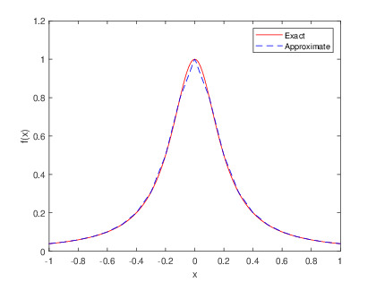
Let us consider the Runge function on [1,1]11[-1,1], that is f4(x)=11+25x2subscript𝑓4𝑥1125superscript𝑥2\displaystyle f_{4}(x)=\frac{1}{1+25x^{2}}. Figure 4 shows the exact and approximate values of f4subscript𝑓4f_{4} for c=0.01,h=0.1,0.02formulae-sequence𝑐0.010.10.02c=0.01,~{}h=0.1,~{}0.02. In Figure 4, we see that the Runge phenomenon has disappeared by decreasing hh. Relative errors are shown in Figure 5 using the RTH quasi-interpolation operator.
Refer to caption
(a)
Refer to caption
(b)
Figure 4: RTH quasi-interpolation of f4(x)=11+25x2;subscript𝑓4𝑥1125superscript𝑥2f_{4}(x)=\frac{1}{1+25x^{2}}; h=0.10.1h=0.1 (a), h=0.020.02h=0.02 (b), and c=0.01.𝑐0.01c=0.01.
Refer to caption
(a)
Refer to caption
(b)
Refer to caption
(c)
Figure 5: Relative errors: c=0.1𝑐0.1c=0.1 (a), c=0.01𝑐0.01c=0.01 (b), c=0.001𝑐0.001c=0.001 (c), and h=0.02;0.02h=0.02; for the test problem 4.

4.5 Test problem 5 (Gibbs Phenomenon)

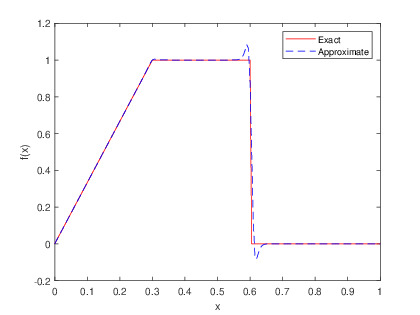
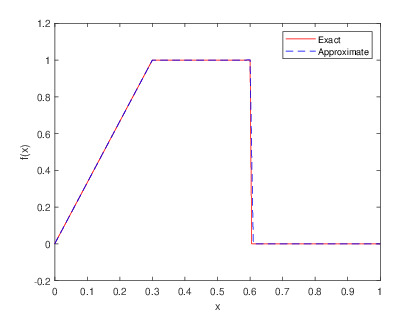
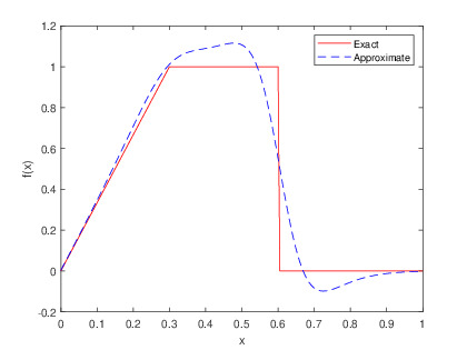
It is well-known that any global or high order approximation method suffers from the Gibbs phenomenon if the function has a jump discontinuity in the given domain. In this test problem, we show that the RTH quasi-interpolation operator substantially mitigates the Gibbs phenomenon (cf. [46]).

f5(x)={103x,0x0.3,1,0.3x0.6,0,0.6<x1.subscript𝑓5𝑥cases103𝑥0𝑥0.310.3𝑥0.600.6𝑥1\displaystyle f_{5}(x)=\left\{\begin{array}[]{ll}\frac{10}{3}x,&0\leq x\leq 0.3,\\ 1,&0.3\leq x\leq 0.6,\\ 0,&0.6<x\leq 1.\end{array}\right.

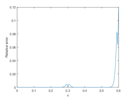
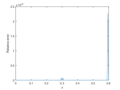
Figure 6 shows the exact and approximate values of f5subscript𝑓5f_{5}. In Figure 6, we see that the Gibbs oscillations are considerably attenuated by decreasing c𝑐c. Relative errors are reported in Figure 7.
Refer to caption
(a)
Refer to caption
(b)
Refer to caption
(c)
Figure 6: Approximations of f5subscript𝑓5f_{5} with RTH quasi-interpolation; c=0.1𝑐0.1c=0.1 (a), c=0.01𝑐0.01c=0.01 (b), c=0.001𝑐0.001c=0.001 (c), and h=0.01.0.01h=0.01.
Refer to caption
(a)
Refer to caption
(b)
Refer to caption
(c)
Figure 7: Relative errors: c=0.1𝑐0.1c=0.1 (a), c=0.01𝑐0.01c=0.01 (b), c=0.001𝑐0.001c=0.001 (c), and h=0.01;0.01h=0.01; Test problem 5.

4.6 Test problem 6 (A piecewise analytic function)

As a final example, we consider the piecewise analytic function (cf. [47])

f6(x)={sin(x),x<0,cos(x),x>0,subscript𝑓6𝑥cases𝑥𝑥0𝑥𝑥0\displaystyle f_{6}(x)=\left\{\begin{array}[]{ll}\sin(x),&x<0,\\ \cos(x),&x>0,\end{array}\right.

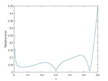
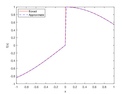
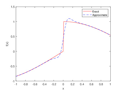
with x[1,1]𝑥11x\in[-1,1]. Figure 8 shows the exact and approximate values of f6subscript𝑓6f_{6}, where Gibbs oscillations are considerably attenuated by decreasing c𝑐c. Relative errors are shown in Figure 9.
Refer to caption
(a)
Refer to caption
(b)
Refer to caption
(c)
Figure 8: RTH quasi-interpolation of the piecewise analytic function f6subscript𝑓6f_{6}; c=0.1𝑐0.1c=0.1 (a), c=0.01𝑐0.01c=0.01 (b), c=0.001𝑐0.001c=0.001 (c), and h=0.02.0.02h=0.02.
Refer to caption
(a)
Refer to caption
(b)
Refer to caption
(c)
Figure 9: Relative errors: c=0.1𝑐0.1c=0.1 (a), c=0.01𝑐0.01c=0.01 (b), c=0.001𝑐0.001c=0.001 (c), and h=0.02;0.02h=0.02; Test problem 6.

5 Conclusion

In this paper, an efficient shape preserving quasi-interpolation operator with high degree of smoothness and very accurate results is proposed. It is based on the reformulation of Wu–Schaback’s quasi-interpolation operator by a new transcendental RBF of the form ϕ(r)=rtanh(rc)italic-ϕ𝑟𝑟𝑟𝑐\phi(r)=r\tanh\left({r\over c}\right). The quasi-interpolation operator, called RTHsubscript𝑅𝑇𝐻{\mathcal{L}}_{RTH} has nice convergence properties, being RTHfkh2subscriptnormsubscript𝑅𝑇𝐻𝑓𝑘superscript2\|{\mathcal{L}}_{RTH}-f\|_{\infty}\leq k\,h^{2}, with hh being the step size and k𝑘k a positive constant independent on the shape parameter c𝑐c and the step size hh (cf. Theorem 3.1). Numerical experiments reveal that the proposed quasi-interpolation operator not only gives very accurate results but also it does not suffer of the Runge and Gibbs phenomena (see Test problems 4-6).
As a future work we are working in the application of the operator to real worlds problems, in particular to irregular surfaces approximation and image segmentation.

Acknowledgments. The third author thanks for the support the GNCS-INdAM. His research has been done within the Italian Network on Approximation (RITA) and the thematic group on "Approximation Theory and Applications" of the Italian Mathematical Union.

References

  • Wendland [2004] Holger Wendland. Scattered data approximation, volume 17. Cambridge university press, 2004.
  • Buhmann [2003] Martin D Buhmann. Radial basis functions: theory and implementations, volume 12. Cambridge university press, 2003.
  • Madych [1992] WR Madych. Miscellaneous error bounds for multiquadric and related interpolators. Computers & Mathematics with Applications, 24(12):121–138, 1992.
  • Madych and Nelson [1989] WR Madych and SA Nelson. Error bounds for multiquadric interpolation. Approximation Theory VI, 2:413–416, 1989.
  • Micchelli [1986] Charles A Micchelli. Interpolation of scattered data: distance matrices and conditionally positive definite functions. Constructive approximation, 2(1):11–22, 1986.
  • Powell [1992a] Michael JD Powell. The theory of radial basis function approximation in 1990. Advances in numerical analysis, pages 105–210, 1992a.
  • Powell [1992b] Michael JD Powell. The theory of radial basis function approximation in 1990. Advances in numerical analysis, pages 105–210, 1992b.
  • Wendland [1995] Holger Wendland. Piecewise polynomial, positive definite and compactly supported radial functions of minimal degree. Advances in computational Mathematics, 4(1):389–396, 1995.
  • Wu [1995] Zongmin Wu. Compactly supported positive definite radial functions. Advances in computational mathematics, 4(1):283–292, 1995.
  • Wu and Schaback [1993] Zong-min Wu and Robert Schaback. Local error estimates for radial basis function interpolation of scattered data. IMA journal of Numerical Analysis, 13(1):13–27, 1993.
  • Fasshauer [1996] Gregory E Fasshauer. Solving partial differential equations by collocation with radial basis functions. In Proceedings of Chamonix, volume 1997, pages 1–8. Citeseer, 1996.
  • Fasshauer [2007] Gregory E Fasshauer. Meshfree approximation methods with MATLAB, volume 6. World Scientific, 2007.
  • Franke and Schaback [1998] Carsten Franke and Robert Schaback. Convergence order estimates of meshless collocation methods using radial basis functions. Advances in computational mathematics, 8(4):381–399, 1998.
  • Golberg et al. [1996] MA Golberg, CS Chen, and SR Karur. Improved multiquadric approximation for partial differential equations. Engineering Analysis with boundary elements, 18(1):9–17, 1996.
  • Hon and Mao [1998] Yiu-Chung Hon and XZ Mao. An efficient numerical scheme for Burgers’ equation. Applied Mathematics and Computation, 95(1):37–50, 1998.
  • Kansa [1990a] Edward J Kansa. Multiquadrics—a scattered data approximation scheme with applications to computational fluid-dynamics—i surface approximations and partial derivative estimates. Computers & Mathematics with applications, 19(8-9):127–145, 1990a.
  • Kansa [1990b] Edward J Kansa. Multiquadrics—a scattered data approximation scheme with applications to computational fluid-dynamics—ii solutions to parabolic, hyperbolic and elliptic partial differential equations. Computers & mathematics with applications, 19(8-9):147–161, 1990b.
  • Mohammadi et al. [2014] M Mohammadi, R Mokhtari, and R Schaback. A meshless method for solving the 2d brusselator reaction-diffusion system. Comput. Model. Eng. Sci.(CMES), 101:113–138, 2014.
  • Saberi Zafarghandi et al. [2019] Fahimeh Saberi Zafarghandi, Maryam Mohammadi, and Robert Schaback. On the fractional derivatives of radial basis functions: Theories and applications. Mathematical Methods in the Applied Sciences, 42(11):3877–3899, 2019.
  • Wendland [1999] Holger Wendland. Meshless galerkin methods using radial basis functions. Mathematics of computation, 68(228):1521–1531, 1999.
  • Zafarghandi et al. [2019] Fahimeh Saberi Zafarghandi, Maryam Mohammadi, Esmail Babolian, and Shahnam Javadi. Radial basis functions method for solving the fractional diffusion equations. Applied Mathematics and Computation, 342:224–246, 2019.
  • Hardy [1971] Rolland L Hardy. Multiquadric equations of topography and other irregular surfaces. Journal of geophysical research, 76(8):1905–1915, 1971.
  • Hardy [1990] Rolland L Hardy. Theory and applications of the multiquadric-biharmonic method 20 years of discovery 1968–1988. Computers & Mathematics with Applications, 19(8-9):163–208, 1990.
  • Franke [1982] Richard Franke. Scattered data interpolation: tests of some methods. Mathematics of computation, 38(157):181–200, 1982.
  • Beatson and Powell [1992] RK Beatson and MJD Powell. Univariate multiquadric approximation: quasi-interpolation to scattered data. Constructive approximation, 8(3):275–288, 1992.
  • Powell [1990] Michael James David Powell. Univariate multiquadric approximation: reproduction of linear polynomials. In Multivariate Approximation and Interpolation, pages 227–240. Springer, 1990.
  • Wu and Schaback [1994] Zongmin Wu and Robert Schaback. Shape preserving properties and convergence of univariate multiquadric quasi-interpolation. Acta Mathematicae Applicatae Sinica, 10(4):441–446, 1994.
  • Ling [2004] Leevan Ling. A univariate quasi-multiquadric interpolationwith better smoothness. Computers & Mathematics with Applications, 48(5-6):897–912, 2004.
  • Feng and Li [2009] Renzhong Feng and Feng Li. A shape-preserving quasi-interpolation operator satisfying quadratic polynomial reproduction property to scattered data. Journal of computational and applied mathematics, 225(2):594–601, 2009.
  • Wang et al. [2010] Ren-Hong Wang, Min Xu, and Qin Fang. A kind of improved univariate multiquadric quasi-interpolation operators. Computers & mathematics with applications, 59(1):451–456, 2010.
  • Jiang et al. [2011] Zi-Wu Jiang, Ren-Hong Wang, Chun-Gang Zhu, and Min Xu. High accuracy multiquadric quasi-interpolation. Applied Mathematical Modelling, 35(5):2185–2195, 2011.
  • Ling [2005] Leevan Ling. Multivariate quasi-interpolation schemes for dimension-splitting multiquadric. Applied mathematics and computation, 161(1):195–209, 2005.
  • Wu et al. [2015] Ruifeng Wu, Tieru Wu, and Huilai Li. A family of multivariate multiquadric quasi-interpolation operators with higher degree polynomial reproduction. Journal of Computational and Applied Mathematics, 274:88–108, 2015.
  • Gao and Wu [2012] Wenwu Gao and Zongmin Wu. Quasi-interpolation for linear functional data. Journal of Computational and Applied Mathematics, 236(13):3256–3264, 2012.
  • Wang and Wu [2007] Renhong Wang and Jinming Wu. Approximate implicitization based on rbf networks and mq quasi-interpolation. Journal of Computational Mathematics, pages 97–103, 2007.
  • Wu and Zhang [2014] Jinming Wu and Xiaolei Zhang. A new approach for approximate implicitization of parametric curves. Computational and Applied Mathematics, 33(2):399–409, 2014.
  • Hon and Wu [2000] YC Hon and Zongmin Wu. A quasi-interpolation method for solving stiff ordinary differential equations. International Journal for Numerical Methods in Engineering, 48(8):1187–1197, 2000.
  • Chen and Wu [2006] Ronghua Chen and Zongmin Wu. Applying multiquadric quasi-interpolation to solve burgers’ equation. Applied mathematics and computation, 172(1):472–484, 2006.
  • Chen and Wu [2007] Ronghua Chen and Zongmin Wu. Solving partial differential equation by using multiquadric quasi-interpolation. Applied Mathematics and Computation, 186(2):1502–1510, 2007.
  • Jiang and Wang [2012] Zi-Wu Jiang and Ren-Hong Wang. Numerical solution of one-dimensional sine–gordon equation using high accuracy multiquadric quasi-interpolation. Applied Mathematics and Computation, 218(15):7711–7716, 2012.
  • Ramirez et al. [2013] Carlos Ramirez, Reinaldo Sanchez, Vladik Kreinovich, and Miguel Argaez. (x2+μ)\sqrt{(}x^{2}+\mu) is the most computationally efficient smooth approximation to |x|: a proof. 2013.
  • Voronin et al. [2014] Sergey Voronin, Gorkem Ozkaya, and Davis Yoshida. Convolution based smooth approximations to the absolute value function with application to non-smooth regularization. arXiv preprint arXiv:1408.6795, 2014.
  • Wall [2018] Hubert Stanley Wall. Analytic theory of continued fractions. Courier Dover Publications, 2018.
  • O’neill [2006] Barrett O’neill. Elementary differential geometry. Elsevier, 2006.
  • Fasshauer and McCourt [2012] Gregory E Fasshauer and Michael J McCourt. Stable evaluation of gaussian radial basis function interpolants. SIAM Journal on Scientific Computing, 34(2):A737–A762, 2012.
  • Chen et al. [2009] Ronghua Chen, Xuli Han, and Zongmin Wu. A multiquadric quasi-interpolation with linear reproducing and preserving monotonicity. Journal of computational and applied mathematics, 231(2):517–525, 2009.
  • Jung [2007] Jae-Hun Jung. A note on the gibbs phenomenon with multiquadric radial basis functions. Applied numerical mathematics, 57(2):213–229, 2007.