Rotating Motion of the Outflow of IRAS 16293–2422 A1 at its Origin Point near the Protostar

Abstract

The Class 0 protostar IRAS 16293–2422 Source A is known to be a binary system (A1 and A2) or even a multiple system, which processes a complex outflow structure. We have observed this source in the C³⁴S, SO, and OCS lines at 3.1 mm with the Atacama Large Millimeter/submillimeter Array (ALMA). A substructure of this source is traced by our high angular-resolution observation (0$\farcs$12; 20 au) of the continuum emission. The northwest-southeast (NW-SE) outflow on a 2″ scale is detected in the SO ($J_{N}$ = $2_{2}$–$1_{1}$) line. Based on the morphology of the SO distribution, this bipolar outflow structure seems to originate from the protostar A1 and its circumstellar disk, or the circummultiple structure of Source A. The rotation motion of the NW-SE outflow is detected in the SO and OCS emissions. We evaluate the specific angular momentum of the outflowing gas to be $(8.6-14.3)\times 10^{-4}$ km s^-1 pc. If the driving source of this outflow is the protostar A1 and its circumstellar disk, it can be a potential mechanism to extract the specific angular momentum of the disk structure. These results can be a hint for the outflow launching mechanism in this source. Furthermore, they provide us with an important clue to resolve the complicated structure of IRAS 16293–2422 Source A.

1 Introduction

In the last decade, the study of disk-formation around solar-type protostars has made extensive progress both theoretically and observationally. In the disk-formation process around a newly-born protostar, outflows/jets and disks are mutually related via the angular momentum. However, their relation has not been elucidated in detail by observations. For instance, there is still difficulty to judge where outflows/jets are launched from; a central protostellar object, an inner-edge of a disk, or a disk surface. Moreover, the outflow launching process in multiple systems is expected to be complex. Since a large fraction of stars are born as a member of a multiple or binary system (e.g. Chen et al. 2013; Duchêne & Kraus 2013; Tobin et al. 2016), investigating jet and outflow structures of binary/multiple systems is essential for the star-formation processes ongoing there.

Outflows/jets from a binary/multiple system have extensively been studied by theoretical magnetohydrodynamics (MHD) simulations and observations. MHD simulations show that an outflow of a binary system can be launched from its circumbinary disk (e.g. Machida et al. 2009; Kuruwita et al. 2017), and that twin jets can arise in a close binary system (Saiki & Machida 2020). Specifically, in addition to the two jets from the two protostars in the latter case, a wide-angle and low-velocity outflow emanates from the structure composed by the circumbinary stream that encloses them. Observations of outflows/jets in binary/multiple systems are not always easy, and the identification of the outflow/jet launching points often requires high angular-resolution observations, particularly for close binary systems. For well-separated binaries, the outflow of each component is often identified, where the two outflows are sometimes parallel (NGC 1333 IRAS 4A, BHR71; Santangelo et al. 2015; Alves et al. 2017) and sometimes not (L1448 IRS3, NGC 2264 CMM3; Tobin et al. 2015; Watanabe et al. 2017). In close binary systems, only one outflow is usually observed. For instance, Alves et al. (2017) reported a wide-angle outflow structure surrounding the binary system BHB 07–11, whose projected separation is 28 au (Alves et al. 2019). This seems to correspond to the low-velocity outflow seen in the recent MHD simulation by Saiki & Machida (2020). To the best of our knowledge, only one close binary system is known having misaligned twin molecular outflows (Hara et al. 2020): VLA 1623A, whose two binary objects are separated by 34 au. Considering the importance of outflows/jets in the formation and evolution of disk structures, high angular-resolution observations of various binary/multiple sources are of fundamental importance.

IRAS 16293–2422 is a Class 0 protostellar source located in Ophiuchus, whose distance from the Solar system is reported to be $(137-147)$ pc by Ortiz-León et al. (2017) and $141^{+30}_{-21}$ pc by Dzib et al. (2018). In this study, we employ 137 pc as the distance to IRAS 16293–2422 (Ortiz-León et al. 2017) for the consistency with the previous analysis (e.g. Oya et al. 2016; Oya & Yamamoto 2020). This source contains two sources (Source A and Source B), which are separated by $\sim 5\arcsec$ ($\sim 700$ au) on the plane of the sky (e.g. Wootten 1989; Mundy et al. 1992; Looney et al. 2000; Chandler et al. 2005; Oya et al. 2016; Jørgensen et al. 2016). Both IRAS 16293–2422 Source A and Source B are known to be prototypical hot corino sources, which are rich in complex organic molecules (COMs), such as CH₃OH (methanol), HCOOCH₃ (methyl formate), (CH₃)₂O (dimethyl ether), and C₂H₅CN (propionitrile) (e.g. van Dishoeck et al. 1995; Cazaux et al. 2003; Schöier et al. 2002; Bottinelli et al. 2004; Kuan et al. 2004; Ceccarelli 2004; Huang et al. 2005; Chandler et al. 2005; Caux et al. 2011; Jørgensen et al. 2011, 2012). Their chemical compositions have extensively been investigated with the Submillimeter Array (SMA; Jørgensen et al. 2011) and the Atacama Large Millimeter/submillimeter Array (ALMA) (e.g. PILS; Protostellar Interferometric Line Survey; Jørgensen et al. 2016; Lykke et al. 2017) as well as with the IRAM 30 m telescope and the James Clerk Maxwell Telescope (JCMT) (Caux et al. 2011).

IRAS 16293–2422 Source A itself is a binary source, or even a multiple source, including at least two protostars A1 and A2 (Wootten 1989; Huang et al. 2005; Chandler et al. 2005; Pech et al. 2010; Hernández-Gómez et al. 2019; Maureira et al. 2020; Oya & Yamamoto 2020 , hereafter OY20). The projected spatial separation between the protostar A1 and A2 is as small as 0$\farcs$36 ($\sim 50$ au; e.g. Hernández-Gómez et al. 2019; Maureira et al. 2020 ; OY20). Moreover, Source A is reported to have substructures other than A1 and A2 (Pech et al. 2010; Hernández-Gómez et al. 2019 ; OY20). Loinard et al. (2013), Pech et al. (2010), and Hernández-Gómez et al. (2019) observed the cm continuum emission with Very Large Array (VLA), and reported a bipolar ejection from the protostar A2.

In this study, we investigate the outflow feature observed toward Source A at a high angular-resolution, corresponding to about 20 au. In Section 2, previous studies of the outflows in IRAS 16293–2422 are summarized, and the principal aim of this paper is presented. Section 3 describes the observation details, and Section 4 the results and discussions, where we particularly focus on the rotation motion of the outflow (Sections 4.3 and 4.5). Finally, in Section 5, we summarize our results.

2 Outflows of IRAS 16293–2422

The outflow structure of IRAS 16293–2422 is quite complicated (see e.g. the review by van der Wiel et al. 2019). Mizuno et al. (1990) and Stark et al. (2004) reported a quadruple outflow structure on a 6′ ($\sim 0.24$ pc) scale extending along the east-west (E-W) and the northeast-southwest (NE-SW) directions. Walker et al. (1988) and Hirano et al. (2001) observed a similar structure over 2′ ($\sim 0.08$ pc). Castets et al. (2001) reported multiple shocks caused by these outflows. On a smaller scale ($\sim 10^{3}$ au scale), outflow structures from the individual components (Source A and Source B) have been observed. A nearly pole-on outflow structure of Source B was suggested by Loinard et al. (2013) and Oya et al. (2018). Meanwhile, Source A is known to have two bipolar outflow structures on a $10^{3}$ au scale. Yeh et al. (2008) detected the E-W outflow in the CO ($J$ = 2–1; $J$ = 3–2) lines, and Loinard et al. (2013) reported that the CO ($J$ = 6–5) line traces the central part of this outflow within 1″ around Source A. van der Wiel et al. (2019) delineated the northwest-southeast (NW-SE) outflow in the SiO ($J$ = 8–7) and H¹³CN ($J$ = 4–3) lines. Both the E-W outflow and the NW-SE outflow were detected by Rao et al. (2009) in the CO ($J$ = 3–2) line, the SiO ($J$ = 8–7) line, and the H¹³CO⁺ ($J$ = 4–3) line, by Kristensen et al. (2013) in the CO ($J$ = 6–5) line, and by Girart et al. (2014) in the CO ($J$ = 3–2) line and the SiO ($J$ = 8–7) line.

The E-W outflow on a $10^{3}$ au scale is blue-shifted and red-shifted on the eastern and western sides of Source A, respectively (Yeh et al. 2008; Rao et al. 2009; Kristensen et al. 2013; Girart et al. 2014). This feature is the same as that seen on the arcminute-scale outflow structure (Walker et al. 1988; Mizuno et al. 1990; Stark et al. 2004). The NW-SE outflow is blue-shifted and red-shifted on the NW and SE sides of Source A, respectively, at the distance of $\sim 5\arcsec$ ($\sim 700$ au) from Source A (Rao et al. 2009; Girart et al. 2014; van der Wiel et al. 2019). Interestingly, it shows the opposite feature at the distance of $\sim 1\arcsec$ ($\sim 140$ au) from Source A (Kristensen et al. 2013).

The E-W outflow has been reported to originate from the protostar A2 based on the proper motion study of the bipolar ejecta from A2 in the cm continuum emission (Loinard et al. 2013; Pech et al. 2010; Hernández-Gómez et al. 2019). On the contrary, the driving source of the NW-SE outflow is still unclear. In this study, we focus on the NW-SE outflow structure of IRAS 16293–2422 Source A, and present new high angular-resolution ($\sim 20$ au) observations resolving the substructure in Source A with ALMA. We investigate the kinematic structure of this outflow near its launching point by using the C³⁴S, SO, and OCS lines.

3 Observation

The ALMA observation of IRAS 16293–2422 was carried out on November 16th and 28th, 2017 during its Cycle 5 operation (#2017.1.01013.S). The 3.1 mm continuum and the rotational spectral lines of C³⁴S ($J$ = 2–1), SO ($J_{N}$ = $2_{2}$–$1_{1}$), and OCS ($J$ = 7–6) were observed with the Band 3 receiver. The observed spectral lines are summarized in Table 1.

In this observation, the field center was set at $(\alpha_{\rm ICRS},\delta_{\rm ICRS})=(16^{\rm h}32^{\rm m}22\fs 79,-24\arcdeg 28\arcmin 34\farcs 30)$, which is the intermediate position of IRAS 16293–2422 Source A and Source B. Forty-three antennas were used during the observations, and their baseline lengths ranged from 92 to 8282 m. The size of the field of view was from 61″ to 71″ and the maximum recoverable scale was from 2$\farcs$3 to 2$\farcs$9 according to the quality assurance report, both of which depend on the frequency. The on-source integration time was 113 minutes in total. Seven spectral windows shown in Table 2 were observed. The bandpass and flux calibrations were performed with J1427–4206. The phase calibration was carried out with J1633–2557 every 12 minutes. The accuracy of the flux density calibration for the target source image is typically expected to be 1% (ALMA Partnership 2017).

The continuum and line images were obtained with the CLEAN algorithm by using CASA (Common Astronomy Software Applications package; McMullin et al. 2007). We employed the Briggs weighting with a robustness parameter of 0.5, unless otherwise noted. The 3.1 mm continuum image was prepared by averaging line-free channels with a cumulative frequency-range of 65.43 MHz. The line images were obtained after subtracting the continuum component directly from the visibility data. The line images were resampled to make the channel width to be 0.2 km s^-1. A primary beam correction was applied to the continuum and line images. Self-calibration was carried out for the phase and amplitude by using the continuum data and was applied to the line data. The synthesized beam size and the root-mean-square (rms) noise level for the continuum image or each molecular line image are summarized in Table 2.

4 Results and Discussions

4.1 Distributions

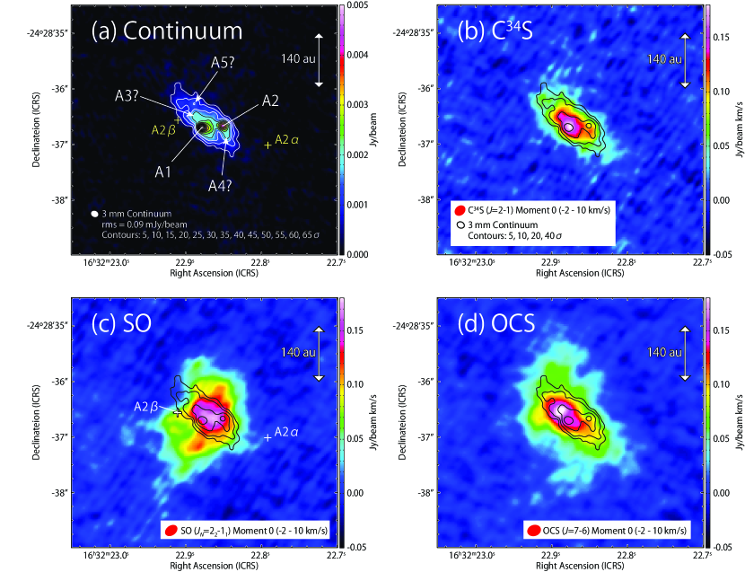
Figure 1: The 3.1 mm continuum image (a) and the integrated intensity maps of the C³⁴S ($J$ = 2–1; b), SO ($J_{N}$ = $2_{2}$–$1_{1}$; c), and OCS ($J$ = 7–6; d) lines. Contours represent the continuum image. Contour levels are every 5$\sigma$ in panel (a), while they are 5, 10, 20, and 40$\sigma$ in the other panels. The rms noise level is 0.09 mJy beam^-1. In panels (b), (c), and (d), the velocity range for the integration is from $-2$ to 10 km s^-1, which corresponds to the velocity shift from $-5.9$ to $+6.1$ km s^-1 for the systemic velocity of the circummultiple structure (3.9 km s^-1). Two crosses in panel (a) show the expected positions of the two ejecta (A2$\alpha$ and A2$\beta$) on our 1st observation date (2017.88) estimated by extrapolating their proper motions from their positions on 2014.15 reported by Hernández-Gómez et al. (2019).

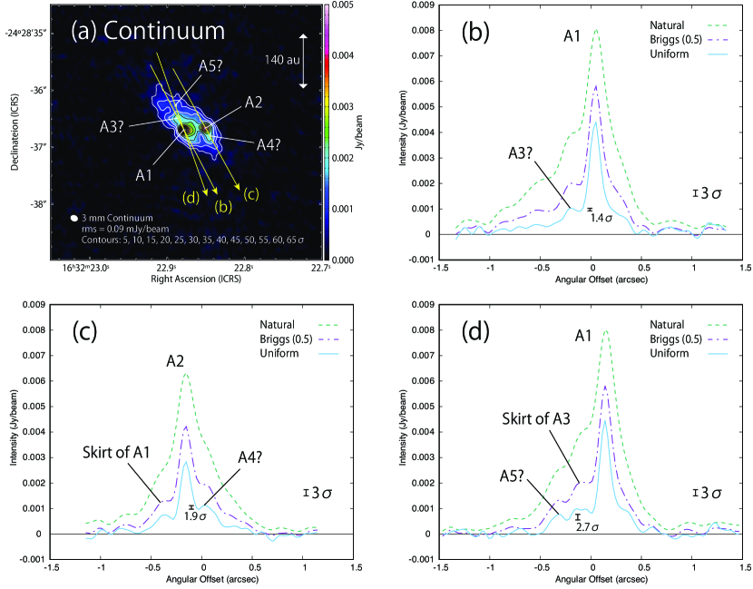
Figure 2: The 3.1 mm continuum image (a) and its spatial profiles (b–d). Panel (a) is the same as panel (a) in Figure 1. Spatial profiles are prepared along the arrows shown in panel (a). The arrows pass through the positions of the intensity peak candidates. The spatial profiles are prepared for the continuum images with the robustness parameter of $+2$ (natural), 0.5, and $-2$ (uniform). The beam size is 0$\farcs$197 $\times$ 0$\farcs$162, 0$\farcs$136 $\times$ 0$\farcs$112, and 0$\farcs$114 $\times$ 0$\farcs$070, with the robustness parameter of $+2$, 0.5, and $-2$, respectively. The three intensity peaks (A3, A4, and A5) are tentatively detected by less than $3\sigma$ in the image with the uniform weighting. A scale of the 3 $\sigma$ noise level of the image with the uniform weighting is depicted in the bottom left corner in each panel, where the rms noise level is 0.9 mJy beam^-1.

Figure 1(a) shows the 3.1 mm continuum image. The continuum emission shows an elliptical distribution with a major-axis diameter of $\sim$ 1$\farcs$5 ($\sim$ 210 au) extending along the NE-SW direction. It can be regarded to trace the circummultiple disk/envelope system of IRAS 16293–2422 Source A, whose mid-plane is reported to extend along the position angle (P.A.) of 50° (OY20). Two intensity peaks (A1 and A2) are clearly seen. Their coordinates are summarized in Table 3, which well correspond to those found in previous observations (e.g. Wootten 1989; Chandler et al. 2005; Pech et al. 2010; Hernández-Gómez et al. 2019; Maureira et al. 2020 ; OY20). In addition, three faint intensity peaks are found by using the 2D Fit Tool of CASA viewer (Table 3) with an intensity excess less than $2\sigma$ (Figure 2). Even with the uniform weighting, the intensity excess is less than $3\sigma$, as shown in the spatial profiles along the lines passing through the continuum peak positions. Two of them are close to the peaks A3 and A4 detected in the 1.3 mm continuum image (OY20). The bipolar ejecta from the protostar A2 found in the cm observation (A2$\alpha$, A2$\beta$; Hernández-Gómez et al. 2019) are not detected in the 3.1 mm continuum image.

Figures 1(b), (c), and (d) show the integrated intensity maps of the C³⁴S ($J$ = 2–1), SO ($J_{N}$ = $2_{2}$–$1_{1}$), and OCS ($J$ = 7–6) lines. The distribution of the C³⁴S emission is similar to that of the 3.1 mm continuum emission (Figure 1b). On the contrary, the SO emission protrudes from the continuum distribution toward the NW and SE directions (Figure 1c). This elongation is perpendicular to the mid-plane of the disk/envelope system (P.A. 50°). On this scale, the SO emission morphologically seems to trace the bipolar outflow blowing along the NW-SE direction previously reported by Rao et al. (2009), Kristensen et al. (2013), Girart et al. (2014), and van der Wiel et al. (2019). The OCS emission is slightly more extended along the disk/envelope system than the 3.1 mm continuum image and the C³⁴S emission (Figure 1d). It would partly trace the NW-SE outflow structure in addition to the extended envelope gas.

The difference in the morphological size of the emitting region of the observed molecular lines is probably due to spatial differentiation of molecular abundances, as well as the excitation conditions of the used lines. The critical density ($n_{\rm crit}$) for the excitation is evaluated to be $\sim(4-5)\times 10^{5}$ cm^-3 for the C³⁴S ($J$ = 2–1) line, $\sim 2\times 10^{5}$ cm^-3 for the SO ($J_{N}$ = $2_{2}$–$1_{1}$) line, and $\sim 2\times 10^{4}$ cm^-3 for the OCS ($J$ = 7–6) line by using their Einstein A coefficients and state-to-state collisional rate coefficients (Yamamoto 2017). The collisional rate coefficients are originally reported by Lique et al. (2006a, b) and Green & Chapman (1978) for the SO, C³⁴S, and OCS lines, respectively. We use the values which are calculated based on the original data and summarized in Leiden Atomic and Molecular Database (LAMDA; Schöier et al. 2005). The Einstein A coefficients are also taken from LAMDA, except for the one of the C³⁴S ($J$ = 2–1) line which is calculated from its line parameters (Table 1). Here, we assume that the collisional rate coefficients of C³⁴S can be approximated by those of C³²S.

In addition to the NW-SE outflow, IRAS 16293–2422 Source A is known to have an outflow blowing along the E-W direction, according to the CO ($J$ = 3–2) observations by Girart et al. (2014). Such a structure is not evident in our SO and OCS observations (Figures 1c, d) and the reason for the non-detection is not clear. This might be due to the difference of the molecular abundances which are highly dependent on the physico-chemical conditions and the age of the shocks (Wakelam et al. 2004). In addition, the excitation effect may contribute to the non-detection of the E-W outflow. The SO ($J_{N}$ = $2_{2}$–$1_{1}$) line has a higher critical density than the CO ($J$ = 3–2) line ($n_{\rm crit}$ $=(2\times 10^{3}-2\times 10^{4})$ cm^-3; Yang et al. 2010), while the OCS ($J$ = 7–6) line has a similar critical density to the CO ($J$ = 3–2) line. A combination of these two effects as well as a resolving-out effect in the interferometric observation would be a cause of the non-detection.

4.2 Kinematic Structures of the Molecular Lines

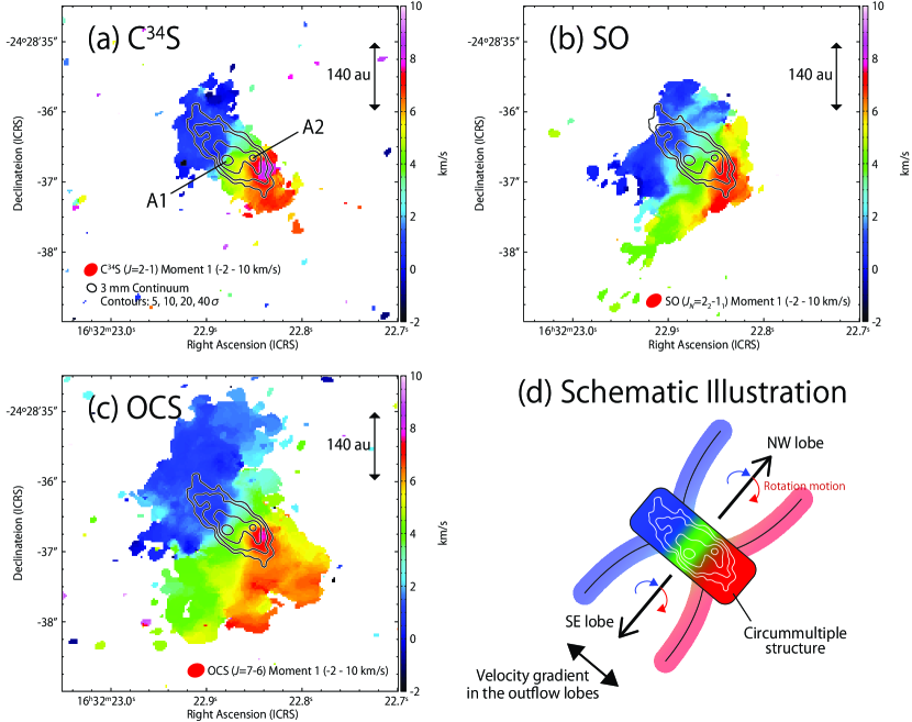
Figure 3: Velocity maps (moment 1 maps) of the C³⁴S ($J$ = 2–1; a), SO ($J_{N}$ = $2_{2}$–$1_{1}$; b), and OCS ($J$ = 7–6; c) lines. Contours represent the 3.1 mm continuum image, where the contour levels are as the same as those in panels (b), (c), and (d) in Figure 1. The velocity range for the integration is from $-2$ to 10 km s^-1, which corresponds to the velocity shift from $-5.9$ to $+6.1$ km s^-1 for the systemic velocity of 3.9 km s^-1. The color maps are prepared by using the data points with the intensity higher than 10 mJy beam^-1 in the datacube; 10 mJy beam^-1 corresponds to 5$\sigma$ for the SO line and to $\sim$3$\sigma$ for the C³⁴S and OCS lines. (d) Schematic illustration for the velocity distribution.

Figure 3 shows the velocity (moment 1) maps of the C³⁴S ($J$ = 2–1), SO ($J_{N}$ = $2_{2}$–$1_{1}$), and OCS ($J$ = 7–6) lines. The C³⁴S line clearly traces a velocity gradient along the NE-SW direction (Figure 3a). This is regarded as the rotating motion in the disk/envelope system of IRAS 16293–2422 Source A reported previously (e.g. Pineda et al. 2012; Favre et al. 2014; Oya et al. 2016; Maureira et al. 2020 ; OY20). It seems to trace the circummultiple structure surrounding both the protostars A1 and A2 (OY20).

OY20 have recently reported that IRAS 16293–2422 Source A has a circummultiple structure surrounding both the protostars A1 and A2 and a circumstellar disk associated with the protostar A1. Figure 4 shows the schematic illustration for Source A. According to their result, the innermost radius of the circummultiple structure is 50 au, and the circumstellar disk resides inside it. It is found that the C¹⁷O ($J$ = 2–1) emission mainly tracing the circummultiple structure shows a hole in its distribution around the protostar A1. In contrast, the distribution of the C³⁴S emission shown in Figure 1(b) extends over 200 au in diameter, without the depression near its central position. Thus, the C³⁴S emission seems to trace both the circummultiple and circumstellar structures.

4.3 Rotating Motion of the Outflow

As shown in Section 4.1, the SO emission is extended along the NW-SE outflow beyond the circummultiple structure traced by the continuum and C³⁴S emission. Morphologically speaking, the SO emission seems to trace the outflow, or its cavity wall instead, although it may also trace the surface of a flared envelope gas. In fact, the SO emission has been reported to trace a disk wind in another protostellar system (HH 212; Tabone et al. 2017; Lee et al. 2021).

The SO emission shows a velocity gradient along the NE-SW direction (Figure 3b), which is almost perpendicular to the NW-SE outflow axis. A similar gradient across the NW-SE outflow is also seen in the OCS line (Figure 3c). These features are schematically illustrated in Figure 3(d).

In order to investigate the kinematic structure of the SO ($J_{N}$ = $2_{2}$–$1_{1}$) line, we show the integrated intensity maps for every 4 km s^-1 in Figure 5. Figure 5(a) compares the map integrated from 0 to 4 km s^-1 and that from 4 to 8 km s^-1, which are blue-shifted and red-shifted, respectively, with respect to the systemic velocity (3.9 km s^-1) of the circummultiple structure (Bottinelli et al. 2004 , OY20). Figure 5(b) shows the maps with higher velocity-shift components ($-4-0$ km s^-1 and $8-12$ km s^-1). Although the protostar A2 is located within the outflow structure as shown in Figure 5(a), it is slightly offset from the outflow axis. Thus, the outflow structure seems to be associated with the protostar A1 rather than A2 morphologically. Alternatively, the outflow may be a disk wind from the circummultiple structure (Figure 4). The latter is examined based on the specific angular momentum of the outflow in Section 4.5.4.

Figures 5(b) and (c) show the high velocity-shift ($-4-0$ and $8-12$ km s^-1) components near the protostars A1 and A2. These components would mostly trace the rotating motion of the circummultiple/circumstellar structures. On the other hand, the high-velocity blue-shifted component ($-4-0$ km s^-1) on the SE side of the protostar A1 in Figure 5(b) is naturally interpreted as a part of the outflow structure. Since this component is near the outflow axis, its velocity-shift would be due to the outflowing motion. The NW outflow lobe shows both the red- and blue-shifted high-velocity components.

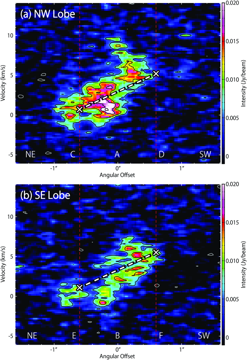
Figure 6: Position-velocity diagrams of the SO ($J_{N}$ = $2_{2}$–$1_{1}$) emission. Their position axes are represented by red arrows in Figure 7(a), which are taken across the outflow axis. The central positions of the position axes are taken at Positions A and B shown in Figure 7. Positions C, D, E, and F are represented by red dashed vertical lines in the diagrams. White crosses in the diagrams represent the velocity centroids obtained by the Gaussian fitting for the spectra at Positions C, D, E, and F (Table 4; Figure 7). The white dashed lines have their ends at the white crosses; they show the overall trend of the velocity gradient across the outflow axis.

Figures 5(a) and (c) clearly show that the NE edges of the bipolar outflow lobes are blue-shifted while their SW edges are red-shifted. This situation is schematically illustrated in Figure 3(d). Such a velocity structure strongly suggests a velocity gradient across the outflow lobes. The gradient can indeed be seen in the velocity (moment 1) maps for the SO and OCS lines (Figures 3b, c). We can also confirm a clear velocity gradient in the position-velocity (PV) diagrams of the SO emission (Figure 6). The position axes of the diagrams are taken across the outflow axis. A velocity gradient along the NE-SW direction is clearly seen in both the NW and SE outflow lobes; the NE parts of the two lobes are blue-shifted, while the SW parts are red-shifted. This is consistent with what we see in Figure 5.

Such features in outflows have been reported, for instance, for the Source I in Orion Kleinmann-Low (Hirota et al. 2017), L483 (Oya et al. 2018), NGC 1333 IRAS 4C (Zhang et al. 2018), and HH 212 (Tabone et al. 2020; Lee et al. 2021). They are interpreted as the rotating motion of the outflows, where the outflow blows nearly perpendicular to the line of sight. It is most likely that the gradient seen in the outflow part of the SO and OCS emission (Figures 3b, c) in the NW-SE outflow is ascribed to its rotating motion.

4.4 Direction of the Outflow

Since the NW-SE outflow blows along the direction nearly perpendicular to the line of sight, the velocity structure near the protostar shows a complex feature due to the contribution from both of the outflowing motion and the rotating motion of the outflow. To investigate the direction of the NW-SE outflow lobes, we consider the spectra of SO at a few positions (Figure 7). We confirm that the SO line in our observation is free from contaminations by other molecular lines according to molecular databases (JPL and CDMS; Pickett et al. 1998; Müller et al. 2005), although this hot corino is rich in COM lines. Figure 7(b) shows the spectra on the outflow axis in the NW and SE outflow lobes. In Figure 5(b), the NW lobe shows both red- and blue-shifted components, while the SE lobe shows only a blue-shifted component. As well, both red- and blue-shifted components are clearly confirmed for the NW lobe in Figure 7(b). For the SE lobe, we detect a red-shifted component weakly but certainly in addition to a clear blue-shifted component, although they overlap each other. The velocity centroids of these four components on the outflow axis are evaluated by the Gaussian fitting (Table 4). The velocity centroids are more blue-shifted in the SE lobe than in the NW lobe.

The more blue-shifted component on the SE side of Source A is consistent with the report by Kristensen et al. (2013), where this component was detected in the CO ($J$ = 6–5) line within 1″ ($\sim 140$ au) around Source A. As described in Section 2, the NW-SE outflow shows the opposite direction on a larger scale ($\sim 5\arcsec$, $\sim 700$ au; Rao et al. 2009; Girart et al. 2014; van der Wiel et al. 2019). A part of the previous observations show that the NW-SE outflow lobes have both blue-shifted and red-shifted components as shown in our observation; the SiO observation by Rao et al. (2009) (their Figure 6), the H₂CO, H${}_{2}^{13}$CO, SiO, and H¹³CN lines by van der Wiel et al. (2019) (their Figure 3). Loinard et al. (2013) and Girart et al. (2014) also detected the red- and blue-shifted components on the NW and SE sides of Source A, respectively. This trend is consistent with our observation and the CO observation by Kristensen et al. (2013).

Combining previous observations with ours, the NW-SE outflow seems to blow almost in parallel to the plane of the sky in the vicinity of Source A on a $<$500 au scale. In this case, both the red- and blue-shifted components come from the back and front sides of the expanding outflow structure. The outflow axis may slightly be tilted from the plane of the sky, where the NW and SE lobes blow away from and toward us, respectively.

In addition, the outflow may have precession and its direction can vary according to the distance from Source A. Since the disk/envelope system of Source A has a complex structure, temporal variation of the outflow direction may occur. These situations make it further complicated to discuss the direction of the outflow axis. Nevertheless, the conclusion that the NW-SE outflow blows almost parallel to the plane of the sky is robust and is consistent with the nearly edge-on circummultiple/circumstellar structures of this source (OY20).

One may think that the SO ($J_{N}$ = $2_{2}$–$1_{1}$) emission comes from the root of the E-W outflow rather than the NW-SE outflow as suggested by Loinard et al. (2013) and Girart et al. (2014). The E-W outflow is thought to cause the bipolar ejecta (A2$\alpha$, A2$\beta$) detected with VLA observations (Hernández-Gómez et al. 2019). The positions of the ejecta are shown in Figure 5(c). A2$\alpha$ is out of our SO emission, although A2$\beta$ is within it; the ejecta are located on the eastern and western sides of Source A, while the SO emission extends along the NW-SE direction from Source A. Considering their positional relation, our SO emission does not likely trace the root of the E-W outflow on this scale, but the NW-SE outflow.

4.5 Specific Angular Momentum

4.5.1 Launching Radius of the NW-SE Outflow Lobes

Figures 7(c) and (d) are the spectra on the edges of the outflow lobes. We show the spectra toward the four positions depicted in Figure 7(a). These spectra are fitted by Gaussian profiles, and the fitting results including their velocity centroids are summarized in Table 4. The velocity gradient inferred from the obtained velocities at Positions C and D is shown by a dashed line in Figure 6(a), while that at Positions E and F is shown in Figure 6(b). The dashed lines well trace the overall trend in the position-velocity diagrams.

The outflowing motion should equally contribute to the velocity centroids at the NE and SW edges in each outflow lobe, so that its contribution can be eliminated approximately by taking the difference of the velocity centroids between the two edges. As well, a possible infall motion can be eliminated. Thus, the rotation velocity of an outflow lobe is obtained as:

$$v_{\rm rot}=\frac{\left|v_{\rm NE}-v_{\rm SW}\right|}{2\sin i},$$ (1)

where $v_{\rm NE}$ and $v_{\rm SW}$ denote the velocity centroids of the spectra on the NE and SW edges, respectively, and $i$ the inclination angle of the outflow (0° for a pole-on configuration). Using the derived velocity difference (Table 4; Figure 7), $v_{\rm rot}$ is evaluated to be $2.25\pm 0.07$ km s^-1 and $2.21\pm 0.06$ km s^-1 for the NW and SE lobes, respectively.

The launching radius of the outflowing gas is often derived from its rotating motion (e.g. Zhang et al. 2018). Anderson et al. (2003) gave the equation to derive a launching radius of a magneto-centrifugal wind ($\varpi_{0}$) (their equation (5)):

$$\varpi_{0}\sim 0.7\left(\frac{\varpi_{\infty}}{10\ {\rm au}}\right)^{2/3}\left(\frac{v_{\phi,\infty}}{10\ {\rm km\ s}^{-1}}\right)^{2/3}\left(\frac{v_{p,\infty}}{100\ {\rm km\ s}^{-1}}\right)^{-4/3}\left(\frac{M}{1\ M_{\odot}}\right)^{1/3}\ {\rm au},$$ (2)

where $\varpi_{\infty}$, $v_{\phi,\infty}$, and $v_{p,\infty}$ denote the distance from the outflow axis, the rotation velocity, and the poloidal velocity at a position far from the launching point, respectively, while $M$ denotes the protostellar mass. Since the poloidal velocity of the outflow of IRAS 16293–2422 Source A is highly uncertain due to the outflow direction almost parallel to the plane of the sky, we here assume a large variety of a poloidal velocity of 3, 10, and 30 km s^-1 as its reasonable range. Then, the launching radius of the NW outflow lobe of IRAS 16293–2422 Source A is calculated to be $83\pm 2$, $16.7\pm 0.4$, and $3.87\pm 0.08$ au, respectively. Here, we employed the rotation velocity of the outflow derived above and the protostellar mass of 0.4 $M_{\odot}$ for the protostar A1 (OY20). Employing the central mass of 1.0 $M_{\odot}$ for Source A (OY20) instead, the launching radius is calculated to be $133\pm 2$, $22.7\pm 0.5$, and $5.3\pm 0.1$ au. Unfortunately, due to the high uncertainties of the poloidal velocity of the outflow and the protostellar mass, the launching radius is not well constrained by this method. The estimation obtained here only gives the practical upper limit of 133 au. Its improvement is left for future study. Therefore, we just discuss whether the outflow can contribute to the extraction of the angular momentum from the disk/envelope system in the following sections.

4.5.2 Specific Angular Momentum of the NW-SE Outflow Lobes

The specific angular momentum ($j$) of the gas is related to the rotation velocity and the distance ($d$) between the NE and SW edges of an outflow lobe, i.e. the diameter of the outflow lobe as:

$$j=v_{\rm rot}\times\frac{d}{2}.$$ (3)

Using the rotation velocity ($v_{\rm rot}$) obtained in Section 4.5.1, we evaluate the specific angular momentum of the gas in the NW and SE outflow lobes rotating around the outflow axis to be ${\displaystyle(9.0\pm 0.3)\times 10^{-4}}$ km s^-1 pc and ${\displaystyle(8.8\pm 0.2)\times 10^{-4}}$ km s^-1 pc, respectively, where the outflow lobes are assumed to be parallel to the plane of the sky ($i$ = 90°).

We here note a caveat on the uncertainty of the inclination angle of the outflow. If the outflow lobes are inclined from the plane of the sky ($i<$ 90°), the above values of the specific angular momentum should be divided by $\sin i$ as described in the equation (1). Thus, they should be regarded as underestimations. According to OY20, the reasonable range of the inclination angle is from 70° to 90° for the circummultiple structure and from 40° to 70°  for the circumstellar disk. Employing these ranges of the inclination angle, the specific angular momentum of the outflow lobes are modified, as summarized in Table 5.

We also perform a similar analysis for the OCS ($J$ = 7–6) line. The details for the results are described in Appendix A. The velocity gradients across the outflow lobes found in the SO emission are confirmed in the OCS emission, and thus the derived specific angular momenta are almost consistent with those derived from the SO emission within a factor of 2 (See Appendix A for more detailed comparison).

4.5.3 Specific Angular Momentum of the Circummultiple Structure of Source A and the Circumstellar disk of the Protostar A1

OY20 have recently reported the kinematic structure of the circummultiple system of Source A and that of the circumstellar disk around the protostar A1 at a spatial resolution of $\sim$ 0$\farcs$1 (14 au). The specific angular momentum of these two structures can be evaluated by using the physical parameters (the protostellar mass, the inclination angle, and the radius of the centrifugal barrier) obtained in their model analysis.

According to OY20, the circummultiple structure of Source A is reproduced by an envelope model with a constant specific angular momentum. The specific angular momentum ($j$) is obtained by using the protostellar mass ($M$) and the radius of the centrifugal barrier ($r_{\rm CB}$) as:

$$j=\sqrt{2GMr_{\rm CB}},$$

where $G$ denotes the gravitational constant (Oya et al. 2014). The results are summarized in Table 5.

Meanwhile, the circumstellar disk of the protostar A1 is reported to be reproduced by a Keplerian disk model. If the gas has a Keplerian rotation with a radius of $r$ from the central protostar with the mass of $M$, its specific angular momentum is obtained as:

$$j=\sqrt{rGM}.$$

The radius of the circumstellar disk is a bit uncertain. It is 30 au based on the H₂CS observation, while its upper limit is 50 au based on the inner most radius of the circummultiple structure surrounding the circumstellar disk. Hence, we evaluate the specific angular momentum for the three cases (the radius of 10, 30, and 50 au), considering the uncertainty of the launching point of the outflow. Again, the results are summarized in Table 5.

It should be noted that the physical parameters of the models employed in the above calculations are highly correlated with each other as demonstrated by OY20 (See Tables A1–4 in their paper). In Table 5, the specific angular momentum values are corrected for the effect of the inclination angle, and the uncertainty of the other physical parameters are taken into account.

4.5.4 Comparison between the Outflow and the Circummultiple/circumstellar Structures

The evaluated specific angular momentum of the NW-SE outflow is larger than that of the circumstellar disk of the protostar A1 (Table 5). In Appendix A, we confirm that this conclusion does not change critically, even if we employ the OCS line instead of the SO line. The conclusion does not change either for the reference positions of $\pm$1″ instead of $\pm$0$\farcs$6. Hence, the result is quite robust. If the driving source of this outflow structure is the protostar A1 and its associated disk, the outflow likely plays an important role in extracting the specific angular momentum of the disk structure, which allows the gas to accrete onto the protostar.

To investigate the angular momentum transportation more quantitatively, we need to consider the transportation of the gas mass in addition to the specific angular momentum. Maureira et al. (2020) have recently reported the gas mass of $(0.001-0.003)$ $M_{\odot}$ and $(0.03-0.1)$ $M_{\odot}$, for the substructure around the protostar A1 and the extended structure surrounding both of A1 and A2, respectively. On the other hand, it is difficult to evaluate the gas mass of the outflow from our observation result. Therefore, we present only a little thought to the balance of the angular momentum between the outflow and the disk/envelope system with rough assumptions. If the gas mass of the outflow were similar to that of the circumstellar disk, the NW-SE outflow could extract $(12-61)$ % of specific angular momentum of the infalling gas onto the disk (See Appendix B for details). Thus, the NW-SE outflow can be one of the mechanisms for the angular momentum loss of the circumstellar disk.

Alternatively, the outflow may be a disk wind from the circummultiple structure of Source A (Section 4.3). For instance, Bjerkeli et al. (2016) reported the CO observation tracing the outflow of the Class I low-mass protostellar source TMC-1A; the wide-angle outflow structure was interpreted as an extended disk wind. In our observation, the SO and OCS lines may trace a similar structure to the disk wind of TMC-1A (Figures 1, 3). In Table 5, the specific angular momentum of the outflow seems slightly smaller than that of the circummultiple structure, and thus, the outflow may not play an effective role to extract the specific angular momentum of the infalling gas. However, the above estimations of the specific angular momentum suffer from uncertainties of the physical parameters, and it would be too hasty to conclude with the current observational results (See Appendix B).

It should be noted that the observed SO distribution may represent the outflow cavity wall rather than the outflowing gas itself, as mentioned in Section 4.3. If this is the case, the observed rotating velocity can be smaller than the actual velocity of the outflowing gas, which leads underestimation of its specific angular momentum. Then, the outflow may have a specific angular momentum larger than both the circummultiple structure and the circumstellar disk; the outflow can play a role in extracting the angular momentum from the accreting gas, wherever in the disk/envelope system the outflow is launched.

As shown in Table 5, the specific angular momentum is different between the circummultiple structure and the circumstellar disk inside it in this source. If the NW-SE outflow does not play a significant role in the extraction of the angular momentum from the cicummultiple structure, another mechanism needs to be considered to account for the observed difference; for instance, a possible transportation of the angular momentum between a binary and its circumbinary disk (e.g. Miranda et al. 2017; Moody et al. 2019; Tiede et al. 2020; Heath & Nixon 2020). This is left for future study.

5 Summary

We have observed the C³⁴S, SO, and OCS line emission as well as the 3.1 mm continuum emission with ALMA toward the Class 0 protostar IRAS 16293–2422 Source A at a resolution from 0$\farcs$12 to 0$\farcs$2 (from 20 to 30 au). We have investigated the kinematic structure of the NW-SE outflow by analyzing the velocity structure of the SO line. The major findings are as follows.

• The substructure of IRAS 16293–2422 Source A is delineated in the 3.1 mm continuum emission. The protostars A1 and A2 are clearly detected. The continuum emission also shows an extended distribution along the NE-SW direction, corresponding to the nearly edge-on disk/envelope system of this source known previously.

• The SO ($J_{N}$ = $2_{2}$–$1_{1}$) emission traces a bipolar outflow structure extending along the NW-SE direction from Source A on a 2″ ($\sim$ 300 au) scale. The C³⁴S ($J$ = 2–1) line traces the rotating disk structure of Source A. It is likely the combination of the circummultiple structure of Source A and the circumstellar disk of the protostar A1. The OCS ($J$ = 7–6) line seems to trace a part of the NW-SE outflow as well as the circummultiple structure and the circumstellar disk.

• The NW-SE outflow blows almost in parallel to the plane of the sky, although its NW and SE lobes would be slightly red- and blue-shifted, respectively.

• The NW-SE outflow does not originate from the protostar A2 based on its morphology, but likely from the protostar A1 and its circumstellar disk, or the circummultiple structure.

• The NW-SE outflow shows a rotating motion in our SO observation. Its specific angular momentum is evaluated to be $(8.7-14.3)\times 10^{-4}$ km s^-1 pc and $(8.6-14.1)\times 10^{-4}$ km s^-1 pc for the NW and SE lobes, respectively, considering the range of inclination angle from 40° to 90° (0° for a pole-on configuration). These values are larger than that of the circumstellar disk of the protostar A1. Thus, this outflow can play a role in the extraction of the specific angular momentum from the disk structure, if its driving source is the protostar A1 and its circumstellar disk. Although the NW-SE outflow does not seem to extract the specific angular momentum from the circummultiple structure of Source A significantly based on the current observational results, we need more accurate observations for a definitive conclusion.

Appendix A Specific Angular Momentum Analysis Using the OCS ($J$ = 7–6) Line

In Section 4.5, we analyze the velocity structure of the SO ($J_{N}$ = $2_{2}$–$1_{1}$) line. In this Section, we perform a similar analysis for the OCS ($J$ = 7–6) line.

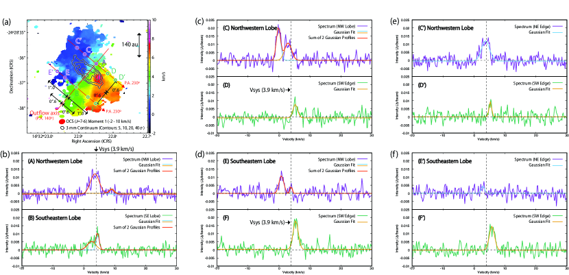
Figure A1: Same as Figure 7 for the OCS ($J$ = 7–6) line. Four positions (C′, D′, E′, F′) are taken at the distance of 1$\farcs$0 (137 au) from Position A or B, as shown in panel (a).

Figure A1 shows the spectra of the OCS line. Since the OCS emission is more extended than the SO emission, we obtain the spectra at four more positions in addition to the six positions employed for the SO analysis. The additional positions (Positions C′, D′, E′, F′) are taken at the distance of 1$\farcs$0 (137 au) from Position A or B. The spectra at the ten positions are fitted by Gaussian profiles, and the fitting results are summarized in Table A1. By using their velocity centroids, we calculate the specific angular momentum of the gas (Table A2). Since the spectra at Positions C and E show a double peak profile, they are fitted by using two Gaussian profiles. Then, the average of the two velocity centroids weighted by the peak intensity is calculated for the velocity at Positions C and E, and is used for the angular momentum calculation. As described in Section 4.5.1, the contamination of the outflowing motion of the gas is expected to be canceled out in the calculation of the specific angular momentum of the gas (equations (1) and (3)), while the contribution of the infalling-rotating envelope may remain.

For the NW outflow lobe, the specific angular momentum calculated by using the OCS line is slightly larger than that calculated by using the SO line by 5 up to 6$\sigma$ at the distance of 0$\farcs$6 (80 au) from the outflow axis (Tables 5, A2). Although the spectrum at Position E′ has a low signal-to-noise ratio, the specific angular momentum obtained for the SE outflow lobe at the distance of 1$\farcs$0 (137 au) from the outflow axis agrees with those obtained in the SO analysis within their uncertainties.

Meanwhile, the specific angular momenta obtained at the distance of 1$\farcs$0 in the NW lobe and at that of 0$\farcs$6 in the SE lobe tend to be lower than those obtained in the SO analysis. Since the OCS emission likely traces the infalling-rotating envelope as well as the NW-SE outflow as described in Section 4.1, the specific angular momenta obtained based on the OCS emission are likely subject to the contamination of the envelope gas. The contribution of the envelope gas would cause a difference between the specific angular momenta obtained in the OCS and SO analyses. In fact, the relatively small specific angular momenta obtained in the OCS analysis just correspond to the intermediate value between the those obtained in the SO analysis and the specific angular momentum of the disk/envelope structures.

Despite the uncertainties mentioned above, the specific angular momenta obtained in the NW-SE outflow lobes tend to be larger than that of the circumstellar disk around the protostar A1, and are likely smaller than that of the circummultiple structure of Source A. A few exceptions happen when we employ the specific angular momentum of the circumstellar disk around the protostar A1 calculated at its upper limit radius (50 au; Table 5). However, it does not change the main conclusion that the NW-SE outflow lobe can contribute to the angular momentum extraction from the circumstellar disk considering that its launching position should be within the outermost edge of the disk (Sections 4.5.4, 5),

Appendix B Balance of the Angular Momentum

When a gas particle falls toward the protostar, it cannot fall inward of its periastron due to the centrifugal force. Thus, infalling gas needs to lose its specific angular momentum for the protostellar evolution. Outflow launching is thought to be one of the candidate mechanism for the angular momentum loss of infalling gas.

The balance of the angular momentum between an outflow and an infalling gas can be formulated as reported by Oya et al. (2018). We consider the case that an infalling gas splits into two gas clumps with a gas mass of $m_{1}$ and $m_{2}$. Then, the balance of the angular momentum among these three gas components is described as:

$$(m_{1}+m_{2})j_{0}=m_{1}j_{1}+m_{2}j_{2},$$ (B1)

where $j_{0}$, $j_{1}$, and $j_{2}$ denote the specific angular momenta of the infalling gas and the two gas clumps.

Here, we suppose that the gas clump with the mass of $m_{1}$ and the specific angular momentum of $j_{1}$ to be the outflowing gas. We obtain the ratio of the specific angular momenta between the other two gas clumps as:

$$\frac{j_{2}}{j_{0}}=\frac{m_{1}+m_{2}}{km_{1}+m_{2}},$$ (B2)

where $j_{1}=kj_{2}$. If $k$ is larger than 1, the specific angular momentum of an infalling gas decreases from $j_{0}$ to $j_{2}$ by the outflow launching.

In our observation (Section 4.5), we evaluate $j_{\rm 1}$ to be $(8.7-14.3)\times 10^{-4}$ km s^-1 pc and $(8.6-14.1)\times 10^{-4}$ km s^-1 pc for the NW and SE outflow lobes, respectively, considering the uncertainty of the inclination angle. We also obtained the specific angular momentum of the circummultiple structure of Source A and the circumstellar disk of the protostar A1 as shown in Table 5.

If the outflow launches from the circumstellar disk, $k$ is evaluated to be from 1.3 to 4.1. Maureira et al. (2020) have recently reported the gas mass of $(0.001-0.003)$ $M_{\odot}$ for the substructure around the protostar A1, and this can be employed as $m_{2}$. If the gas mass of outflow ($m_{1}$) were the same as $m_{2}$, ${\displaystyle\frac{j_{2}}{j_{0}}}$ would be obtained to be from 0.39 to 0.88 by using the equation (B2). In other words, the infalling gas loses from 12 to 61 % of its specific angular momentum ($j_{0}$) by outflow launching, and falls near the protostar A1 to form its circumstellar disk. The infalling gas loses more specific angular momentum for a larger gas mass of outflow, and the upper limit to of the specific angular momentum loss is obtained to be 76 % ${\displaystyle\left(1-\frac{1}{k}\right)}$.

The specific angular momentum of the circummultiple structure seems to be larger than that of the NW-SE outflow. If this is the case, $k$ is smaller than 1, and thus ${\displaystyle\frac{j_{2}}{j_{0}}}$ is larger than 1. In other words, the NW-SE outflow does not seem to extract the specific angular momentum from the circummultiple structure significantly. Nevertheless, the evaluations of the specific angular momentum in our observations would have a large uncertainties. As well, it should be noted that $m_{0}$ and $m_{2}$ depends on where the outflow is launched. This is also highly uncertain with our observations. Therefore, the conclusion for the angular momentum extraction from the circummultiple structure is left for future study.

Table 1: Molecular Lines

Molecule	Transition	Rest Frequency	S$\mu^{2}$	$E_{\rm u}$
		(GHz)	($D^{2}$)	(K)
3 mm Continuum		$97.2331-98.1696$
C34S	$J$ = 2–1	96.41294950	7.6	6.2
SO	$J_{N}$ = $2_{2}$–$1_{1}$	86.09395000	3.5	19
OCS	$J$ = 7–6	85.13910320	3.6	16

Table 2: Settings of the Spectral Windows in the Observation

SPW ID	Frequency Range	Resolution	Molecular Lines	Beam Size	RMS
	(GHz)	(kHz)			(mJy beam-1)
0	84.5675–84.5089	30.517
1	85.1795–85.1209	30.517	OCS ($J$ = 7–6)	0$\farcs$250 $\times$ 0$\farcs$199	3
				(P.A. $-71.\!\!\arcdeg 925$)
2	86.1284–86.0699	61.035	SO ($J_{N}$ = $2_{2}$–$1_{1}$)	0$\farcs$245 $\times$ 0$\farcs$173	2
				(P.A. $-54.\!\!\arcdeg 152$)
3	86.8754–86.8169	61.035
4	96.3827–96.4413	30.517	C34S ($J$ = 2–1)	0$\farcs$211 $\times$ 0$\farcs$167	3
				(P.A. $-49.\!\!\arcdeg 137$)
5	97.271–97.3296	61.035
6	97.2331–98.1696	976.555	Continuum	0$\farcs$136 $\times$ 0$\farcs$112	0.09
				(P.A. $64.\!\!\arcdeg 080$)

Table 3: Intensity Peaks in the 3.1 mm Continuum Map

Peak	Peak Intensity (mJy/beam)	RA (ICRS)	Dec (ICRS)
A1	5.98	16h32m22$\fs$879	$-$24°28′36$\farcs$691
A2	4.27	16h32m22$\fs$851	$-$24°28′36$\farcs$660
A3?	2.05	16h32m22$\fs$887	$-$24°28′36$\farcs$493
A4?	1.93	16h32m22$\fs$847	$-$24°28′36$\farcs$802
A5?	1.37	16h32m22$\fs$889	$-$24°28′36$\farcs$266

Table 4: Results of the Gaussian Fitting for the Spectra of the SO ($J_{N}$ = $2_{2}$–$1_{1}$) Line

Position	Distance from	Peak Intensity	Velocity Centroid	FWHM
	the Outflow Axis	(mJy beam-1)	(km s-1)	(km s-1)
Northwestern Outflow Lobe
Center (Position A)	0″	$15.6\pm 0.7$	$2.5\pm 0.1$	$5.3\pm 0.3$
		$9.2\pm 1.0$	$8.7\pm 0.1$	$2.2\pm 0.3$
NE Edge (Position C)	0$\farcs$6 (80 au)	$11.7\pm 0.7$	$0.7\pm 0.1$	$4.2\pm 0.3$
SW Edge (Position D)	0$\farcs$6 (80 au)	$7.4\pm 0.8$	$5.2\pm 0.1$	$2.2\pm 0.3$
Southeastern Outflow Lobe
Center (Position B)	0″	$13.8\pm 0.5$	$1.1\pm 0.1$	$5.0\pm 0.3$
		$5.2\pm 0.9$	$5.5\pm 0.2$	$2.0\pm 0.4$
NE Edge (Position E)	0$\farcs$6 (80 au)	$8.4\pm 0.6$	$1.1\pm 0.1$	$3.9\pm 0.3$
SW Edge (Position F)	0$\farcs$6 (80 au)	$13.1\pm 0.9$	$5.52\pm 0.07$	$2.2\pm 0.2$

Table 5: Specific Angular Momenta of the Outflow Lobes and the Circummultiple/circumstellar Structures

Structure	Distance from	Inclination Angle
	the Outflow Axis	40°	50°	60°	70°	80°	90°
NW Outflow Lobe	80 au	$13.9\pm 0.4$	$11.7\pm 0.4$	$10.4\pm 0.3$	$9.5\pm 0.3$	$9.1\pm 0.3$	$9.0\pm 0.3$
SE Outflow Lobe	80 au	$13.7\pm 0.4$	$11.5\pm 0.3$	$10.2\pm 0.3$	$9.4\pm 0.3$	$8.9\pm 0.2$	$8.8\pm 0.2$
Circummultiple Structure of Source A	$50-300$ au	$-$	$-$	$-$	$14.4$	$12.9-15.8$	$11.2-15.8$
Circumstellar Disk of Protostar A1	10 au	$3.5-4.1$	$2.9-3.5$	$2.9-3.2$	$2.9-3.2$	$-$	$-$
	30 au	$6.1-7.1$	$5.0-6.1$	$5.0-5.6$	$5.0-5.6$	$-$	$-$
	50 au	$7.9-9.1$	$6.5-7.9$	$6.5-7.2$	$6.5-7.2$	$-$	$-$

Figure 4: Schematic illustration of the outflow and the disk/envelope system of IRAS 16293–2422 Source A. The specific angular momentum ($j$) of the gas in each structure is shown in the unit of ($10^{-4}$ km s^-1 pc) (Table 5). Two possibilities for the origin of the NW-SE outflow are presented. (1) The NW-SE outflow structure originates from the protostar A1 and its circumstellar disk, or (2) it is a disk wind from the circummultiple structure of Source A. In this figure, we employ the distance ($d$) of 137 pc (Ortiz-León et al. 2017) to IRAS 16293–2422 from the Sun. The distance between the protostars A1 and A2 is $\sim$50 au on the plane of the sky (e.g. Hernández-Gómez et al. 2019 ; OY20). Its deprojected distance is 95.6 au (Maureira et al. 2020) by employing the inclination angle of 64° (Maureira et al. 2020) and $d$ of 141 pc (Dzib et al. 2018), which corresponds to $\sim$93 au for $d$ of 137 pc. The lower and upper limits to the radius of the circumstellar disk of A1 are 30 au and 50 au, respectively, according to the H₂CS observations by OY20. The existence of a circumstellar disk around A2 is still controversial; Maureira et al. (2020) attributed the H₂CS emission to a possible disk around A2 with a radius of 50 au using $d$ of 141 pc, while OY20 attributed it to a skirt of the disk around A1. The circummultiple structure is traced up to 300 au by the C¹⁷O emission reported by OY20.

Figure 5: Integrated intensity maps of the SO ($J_{N}$ = $2_{2}$–$1_{1}$) line (contours): the low velocity-shift components in panel (a), the high velocity-shift components in panel (b), and the overlap of them in panel (c). Gray-scale maps show the 3.1 mm continuum image. The velocity ranges for integration are shown in the top left corner of each panel: from $-4$ to 0 km s^-1 for the blue contours, from 0 to 4 km s^-1 for the cyan contours, from 4 to 8 km s^-1 for the magenta contours, and from 8 to 12 km s^-1 for the red contours. The systemic velocity of Source A is 3.9 km s^-1. The cyan (0–4 km s^-1) and magenta (4–8 km s^-1) contours are shown in dotted line in panel (c) for clarity. Contour levels are every 3$\sigma$ in panels (a) and (b), and every 5$\sigma$ in panel (c), where the rms noise level is 4 mJy beam^-1 km s^-1. In panel (a), the directions of the outflows on a $10^{3}$ au scale reported previously are shown by four arrows: the E-W bipolar outflow is reported by Yeh et al. (2008) and Loinard et al. (2013), the NW-SE one by van der Wiel et al. (2019), and both by Rao et al. (2009), Kristensen et al. (2013), and Girart et al. (2014). (See Section 2).

Figure 7: (a) Velocity (moment 1) map of the SO ($J_{N}$ = $2_{2}$–$1_{1}$) line. The color map and the contours are the same as those in Figure 3(b). Six circles represent the positions where the spectra of the SO ($J_{N}$ = $2_{2}$–$1_{1}$) line in panels (b), (c), and (d) are taken. Positions A, C, and D are on the northwestern outflow lobe, while positions B, E, and F are on the southeastern lobe. Position A is taken on the outflow axis at the distance of 0$\farcs$6 (80 au) from the protostar A1 on its northwestern side. Positions C and D are taken at the northeastern and southwestern edges of the northwestern lobe, respectively, which are at the distance of 0$\farcs$6 from position A. Positions B, E, and F are as well, for the southeastern lobe. (b) Spectra on the outflow axis taken at positions A (upper panel) and B (lower panel). (c) Spectra in the northwestern lobe taken at positions C (upper panel) and D (lower panel). (d) Spectra in the southeastern lobe taken at positions E (upper panel) and F (lower panel). The result of Gaussian fitting for each spectrum is shown in each panel and summarized in Table 4. Spectra at positions A and B are fitted by two Gaussian profiles, while the others are by one Gaussian profile.

Table A1: Results of the Gaussian Fitting for the Spectra of the OCS ($J$ = 7–6) Line

Position	Distance from	Peak Intensity	Velocity Centroid	FWHM
	the Outflow Axis	(mJy beam-1)	(km s-1)	(km s-1)
Northwestern Outflow Lobe
Center (Position A)	0″	$12.7\pm 0.9$	$3.6\pm 0.1$	$3.4\pm 0.3$
		$2.9\pm 1.2$	$8.9\pm 0.4$	$1.9\pm 0.9$
NE Edge (Position C)	0$\farcs$6 (80 au)	$20.6\pm 1.4$	$-1.28\pm 0.06$	$1.6\pm 0.1$
		$10.8\pm 1.1$	$3.0\pm 0.1$	$2.6\pm 0.4$
NE Edge (Position C′)	1$\farcs$0 (137 au)	$12.6\pm 0.9$	$3.7\pm 0.1$	$3.0\pm 0.3$
SW Edge (Position D)	0$\farcs$6 (80 au)	$8.4\pm 1.2$	$5.3\pm 0.1$	$1.8\pm 0.3$
SW Edge (Position D′)	1$\farcs$0 (137 au)	$9.5\pm 1.7$	$5.26\pm 0.09$	$1.0\pm 0.2$
Southeastern Outflow Lobe
Center (Position B)	0″	$5.3\pm 0.9$	$2.5\pm 0.5$	$3.1\pm 1.1$
		$9.4\pm 2.3$	$4.5\pm 0.9$	$1.1\pm 0.3$
NE Edge (Position E)	0$\farcs$6 (80 au)	$11.0\pm 1.3$	$0.8\pm 0.1$	$1.8\pm 0.2$
		$5.9\pm 2.2$	$4.0\pm 0.1$	$0.6\pm 0.3$
NE Edge (Position E′)	1$\farcs$0 (137 au)	$4.5\pm 1.5$	$2.9\pm 0.2$	$1.2\pm 0.5$
SW Edge (Position F)	0$\farcs$6 (80 au)	$17.7\pm 1.1$	$5.40\pm 0.06$	$1.9\pm 0.1$
SW Edge (Position F′)	1$\farcs$0 (137 au)	$14.7\pm 1.1$	$5.78\pm 0.08$	$2.0\pm 0.2$

Table A2: Specific Angular Momenta of the Outflow Lobes Traced by the OCS ($J$ = 7–6) Line

Structure	Distance from	Inclination Angle
	the Outflow Axis	40°	50°	60°	70°	80°	90°
NW Outflow Lobe	80 au	$15.8\pm 0.4$	$13.3\pm 0.3$	$11.8\pm 0.3$	$10.8\pm 0.2$	$10.3\pm 0.2$	$10.2\pm 0.2$
	137 au	$8.1\pm 0.7$	$6.8\pm 0.6$	$6.0\pm 0.5$	$5.5\pm 0.5$	$5.3\pm 0.5$	$5.2\pm 0.4$
SE Outflow Lobe	80 au	$10.8\pm 0.3$	$9.1\pm 0.2$	$8.0\pm 0.2$	$7.4\pm 0.2$	$7.0\pm 0.2$	$6.9\pm 0.2$
	137 au	$14.9\pm 1.1$	$12.5\pm 0.9$	$11.0\pm 0.8$	$10.2\pm 0.8$	$9.7\pm 0.7$	$9.6\pm 0.7$

References

- ALMA Partnership (2017) ALMA Partnership, 2017, S. Asayama, A. Biggs, I. de Gregorio, B. Dent, J. Di Francesco, E. Fomalont,A. Hales, J. Hibbard, G. Marconi, S. Kameno, B. Vila Vilaro, E. Villard, F. Stoehr, ISBN: 978-3-923524-66-2
- Alves et al. (2017) Alves, F. O., Girart, J. M., Caselli, P., et al. 2017, A&A, 603, L3. doi:10.1051/0004-6361/201731077
- Alves et al. (2019) Alves, F. O., Caselli, P., Girart, J. M., et al. 2019, Science, 366, 90
- Anderson et al. (2003) Anderson, J. M., Li, Z.-Y., Krasnopolsky, R., et al. 2003, ApJ, 590, L107. doi:10.1086/376824
- Bjerkeli et al. (2016) Bjerkeli, P., van der Wiel, M. H. D., Harsono, D., et al. 2016, Nature, 540, 406
- Bottinelli et al. (2004) Bottinelli, S., Ceccarelli, C., Neri, R., et al. 2004, ApJ, 617, L69
- Brinch et al. (2016) Brinch, C., Jørgensen, J. K., Hogerheijde, M. R., et al. 2016, ApJ, 830, L16. doi:10.3847/2041-8205/830/1/L16
- Castets et al. (2001) Castets, A., Ceccarelli, C., Loinard, L., et al. 2001, A&A, 375, 40. doi:10.1051/0004-6361:20010662
- Caux et al. (2011) Caux, E., Kahane, C., Castets, A., et al. 2011, A&A, 532, A23
- Cazaux et al. (2003) Cazaux, S., Tielens, A. G. G. M., Ceccarelli, C., et al. 2003, ApJ, 593, L51
- Ceccarelli (2004) Ceccarelli, C. 2004, Star Formation in the Interstellar Medium: In Honor of David Hollenbach, 323, 195
- Chandler et al. (2005) Chandler, C. J., Brogan, C. L., Shirley, Y. L., et al. 2005, ApJ, 632, 371
- Chen et al. (2013) Chen, X., Arce, H. G., Zhang, Q., et al. 2013, ApJ, 768, 110. doi:10.1088/0004-637X/768/2/110
- Duchêne & Kraus (2013) Duchêne, G. & Kraus, A. 2013, ARA&A, 51, 269. doi:10.1146/annurev-astro-081710-102602
- Dzib et al. (2018) Dzib, S. A., Ortiz-León, G. N., Hernández-Gómez, A., et al. 2018, A&A, 614, A20. doi:10.1051/0004-6361/201732093
- Favre et al. (2014) Favre, C., Jørgensen, J. K., Field, D., et al. 2014, ApJ, 790, 55
- Girart et al. (2014) Girart, J. M., Estalella, R., Palau, A., et al. 2014, ApJ, 780, L11
- Green & Chapman (1978) Green, S. & Chapman, S. 1978, ApJS, 37, 169
- Hara et al. (2020) Hara, C., Kawabe, R., Nakamura, F., et al. 2020, arXiv:2010.06825
- Heath & Nixon (2020) Heath, R. M. & Nixon, C. J. 2020, A&A, 641, A64. doi:10.1051/0004-6361/202038548
- Hernández-Gómez et al. (2019) Hernández-Gómez, A., Loinard, L., Chandler, C. J., et al. 2019, ApJ, 875, 94
- Hirano et al. (2001) Hirano, N., Mikami, H., Umemoto, T., et al. 2001, ApJ, 547, 899. doi:10.1086/318432
- Hirota et al. (2017) Hirota, T., Machida, M. N., Matsushita, Y., et al. 2017, Nature Astronomy, 1, 0146
- Huang et al. (2005) Huang, H.-C., Kuan, Y.-J., Charnley, S. B., et al. 2005, Advances in Space Research, 36, 146. doi:10.1016/j.asr.2005.03.115
- Jørgensen et al. (2011) Jørgensen, J. K., Bourke, T. L., Nguyen Luong, Q., et al. 2011, A&A, 534, A100. doi:10.1051/0004-6361/201117139
- Jørgensen et al. (2012) Jørgensen, J. K., Favre, C., Bisschop, S. E., et al. 2012, ApJ, 757, L4
- Jørgensen et al. (2016) Jørgensen, J. K., van der Wiel, M. H. D., Coutens, A., et al. 2016, A&A, 595, A117
- Kristensen et al. (2013) Kristensen, L. E., Klaassen, P. D., Mottram, J. C., et al. 2013, A&A, 549, L6
- Kuruwita et al. (2017) Kuruwita, R. L., Federrath, C., & Ireland, M. 2017, MNRAS, 470, 1626. doi:10.1093/mnras/stx1299
- Kuan et al. (2004) Kuan, Y.-J., Huang, H.-C., Charnley, S. B., et al. 2004, ApJ, 616, L27
- Lee et al. (2021) Lee, C.-F., Tabone, B., Cabrit, S., et al. 2021, ApJ, 907, L41. doi:10.3847/2041-8213/abda38
- Lique et al. (2006a) Lique, F., Dubernet, M.-L., Spielfiedel, A., et al. 2006, A&A, 450, 399
- Lique et al. (2006b) Lique, F., Spielfiedel, A., & Cernicharo, J. 2006, A&A, 451, 1125. doi:10.1051/0004-6361:20054363
- Loinard et al. (2013) Loinard, L., Zapata, L. A., Rodriguez, L. F., et al. 2013, MNRAS, 430, L10
- Looney et al. (2000) Looney, L. W., Mundy, L. G., & Welch, W. J. 2000, ApJ, 529, 477
- Lykke et al. (2017) Lykke, J. M., Coutens, A., Jørgensen, J. K., et al. 2017, A&A, 597, A53. doi:10.1051/0004-6361/201629180
- Machida et al. (2009) Machida, M. N., Inutsuka, S., & Matsumoto, T. 2009, ApJ, 704, L10. doi:10.1088/0004-637X/704/1/L10
- Maureira et al. (2020) Maureira, M. J., Pineda, J. E., Segura-Cox, D. M., et al. 2020, ApJ, 897, 59
- McMullin et al. (2007) McMullin, J. P., Waters, B., Schiebel, D., et al. 2007, Astronomical Data Analysis Software and Systems XVI, 376, 127
- Miranda et al. (2017) Miranda, R., Muñoz, D. J., & Lai, D. 2017, MNRAS, 466, 1170. doi:10.1093/mnras/stw3189
- Mizuno et al. (1990) Mizuno, A., Fukui, Y., Iwata, T., et al. 1990, ApJ, 356, 184. doi:10.1086/168829
- Moody et al. (2019) Moody, M. S. L., Shi, J.-M., & Stone, J. M. 2019, ApJ, 875, 66. doi:10.3847/1538-4357/ab09ee
- Müller et al. (2005) Müller, H. S. P., Schlöder, F., Stutzki, J., & Winnewisser, G. 2005, Journal of Molecular Structure, 742, 215
- Mundy et al. (1992) Mundy, L. G., Wootten, A., Wilking, B. A., et al. 1992, ApJ, 385, 306. doi:10.1086/170939
- Ortiz-León et al. (2017) Ortiz-León, G. N., Loinard, L., Kounkel, M. A., et al. 2017, ApJ, 834, 141
- Oya et al. (2014) Oya, Y., Sakai, N., Sakai, T., et al. 2014, ApJ, 795, 152
- Oya et al. (2016) Oya, Y., Sakai, N., López-Sepulcre, A., et al. 2016, ApJ, 824, 88
- Oya et al. (2018) Oya, Y., Moriwaki, K., Onishi, S., et al. 2018, ApJ, 854, 96
- Oya et al. (2018) Oya, Y., Sakai, N., Watanabe, Y., et al. 2018, ApJ, 863, 72. doi:10.3847/1538-4357/aacf42
- Oya & Yamamoto (2020) Oya, Y. & Yamamoto, S. 2020, ApJ, 904, 185. doi:10.3847/1538-4357/abbe14
- Pech et al. (2010) Pech, G., Loinard, L., Chandler, C. J., et al. 2010, ApJ, 712, 1403
- Pickett et al. (1998) Pickett, H. M., Poynter, R. L., Cohen, E. A., et al. 1998, J. Quant. Spec. Radiat. Transf., 60, 883
- Pineda et al. (2012) Pineda, J. E., Maury, A. J., Fuller, G. A., et al. 2012, A&A, 544, L7
- Rao et al. (2009) Rao, R., Girart, J. M., Marrone, D. P., et al. 2009, ApJ, 707, 921
- Saiki & Machida (2020) Saiki, Y. & Machida, M. N. 2020, ApJ, 897, L22
- Santangelo et al. (2015) Santangelo, G., Codella, C., Cabrit, S., et al. 2015, A&A, 584, A126. doi:10.1051/0004-6361/201526323
- Schöier et al. (2002) Schöier, F. L., Jørgensen, J. K., van Dishoeck, E. F., & Blake, G. A. 2002
- Schöier et al. (2005) Schöier, F. L., van der Tak, F. F. S., van Dishoeck, E. F., et al. 2005, A&A, 432, 369
- Stark et al. (2004) Stark, R., Sandell, G., Beck, S. C., et al. 2004, ApJ, 608, 341
- Tabone et al. (2017) Tabone, B., Cabrit, S., Bianchi, E., et al. 2017, A&A, 607, L6. doi:10.1051/0004-6361/201731691
- Tabone et al. (2020) Tabone, B., Cabrit, S., Pineau des Forêts, G., et al. 2020, A&A, 640, A82. doi:10.1051/0004-6361/201834377
- Tiede et al. (2020) Tiede, C., Zrake, J., MacFadyen, A., et al. 2020, ApJ, 900, 43. doi:10.3847/1538-4357/aba432
- Tobin et al. (2015) Tobin, J. J., Looney, L. W., Wilner, D. J., et al. 2015, ApJ, 805, 125. doi:10.1088/0004-637X/805/2/125
- Tobin et al. (2016) Tobin, J. J., Kratter, K. M., Persson, M. V., et al. 2016, Nature, 538, 483
- van der Wiel et al. (2019) van der Wiel, M. H. D., Jacobsen, S. K., Jørgensen, J. K., et al. 2019, A&A, 626, A93
- van Dishoeck et al. (1995) van Dishoeck, E. F., Blake, G. A., Jansen, D. J., et al. 1995, ApJ, 447, 760
- Wakelam et al. (2004) Wakelam, V., Castets, A., Ceccarelli, C., et al. 2004, A&A, 413, 609. doi:10.1051/0004-6361:20031572
- Walker et al. (1988) Walker, C. K., Lada, C. J., Young, E. T., et al. 1988, ApJ, 332, 335. doi:10.1086/166659
- Watanabe et al. (2017) Watanabe, Y., Sakai, N., López-Sepulcre, A., et al. 2017, ApJ, 847, 108. doi:10.3847/1538-4357/aa88b6
- Wootten (1989) Wootten, A. 1989, ApJ, 337, 858
- Yamamoto (2017) Yamamoto, S. 2017, Introduction to Astrochemistry: Chemical Evolution from Interstellar Clouds to Star and Planet Formation, Astronomy and Astrophysics Library, by Satoshi Yamamoto. ISBN 978-4-431-54170-7. Springer Japan, 2017
- Yang et al. (2010) Yang, B., Stancil, P. C., Balakrishnan, N., et al. 2010, ApJ, 718, 1062
- Yeh et al. (2008) Yeh, S. C. C., Hirano, N., Bourke, T. L., et al. 2008, ApJ, 675, 454
- Zhang et al. (2018) Zhang, Y., Higuchi, A. E., Sakai, N., et al. 2018, ApJ, 864, 76