Hierarchical Agglomerative Graph Clustering
in Nearly-Linear Time

Abstract

We study the widely used hierarchical agglomerative clustering (HAC) algorithm on edge-weighted graphs. We define an algorithmic framework for hierarchical agglomerative graph clustering that provides the first efficient $\tilde{O}(m)$ time exact algorithms for classic linkage measures, such as complete- and WPGMA-linkage, as well as other measures. Furthermore, for average-linkage, arguably the most popular variant of HAC, we provide an algorithm that runs in $\tilde{O}(n\sqrt{m})$ time. For this variant, this is the first exact algorithm that runs in subquadratic time, as long as $m=n^{2-\epsilon}$ for some constant $\epsilon>0$. We complement this result with a simple $\epsilon$-close approximation algorithm for average-linkage in our framework that runs in $\tilde{O}(m)$ time. As an application of our algorithms, we consider clustering points in a metric space by first using $k$-NN to generate a graph from the point set, and then running our algorithms on the resulting weighted graph. We validate the performance of our algorithms on publicly available datasets, and show that our approach can speed up clustering of point datasets by a factor of 20.7–76.5x.

1 Introduction

Clustering is a fundamental and widely used unsupervised learning technique with numerous applications in data mining, machine learning, and social network analysis. Hierarchical clustering is a popular approach to clustering which outputs a hierarchy of clusters, where the input data objects are singleton clusters at the bottom of the tree, with interior vertices corresponding to merging the two children clusters. In this paper, we consider the family of hierarchical agglomerative clustering (HAC) algorithms, which have attracted significant theoretical and practical attention since they were first proposed nearly 50 years ago [25, 26, 38].

A HAC algorithm takes as input a set of $n$ points and proceeds in $n-1$ steps. In each step, it finds two most similar points and merges them together. Here, the notion of similarity is defined by a configurable linkage measure.

The specific choice of the linkage measure affects both the clustering quality and the computational complexity of the HAC algorithm. In the case of a general linkage measure, HAC can be implemented in $O(n^{3})$ time, assuming that we are given the similarity between each two points as input. For the most commonly used linkage measure (single, average, Ward’s and complete linkage) this complexity can be improved to $O(n^{2})$ by using the nearest-neighbor chain algorithm [4].

The $O(n^{2})$ time algorithms for HAC are often referred to as optimal, given that they take the entire $n\times n$ similarity matrix as the input. However, from a practical point of view, this quadratic lower bound is very pessimistic, as in many applications only a small fraction of the $n\times n$ similarities are non-negligible. As an example, consider the problem of clustering search engine queries studied in [3]. Each query is assigned a set of relevant URLs and the similarity between two queries is based on the overlap between their URL sets. Clearly, for the vast majority of query pairs, the similarity is zero.

Knowing that in practice only $o(n^{2})$ pairs of input points have non-negligible similarity scores results in two natural questions. First, is it possible to design a subquadratic HAC algorithm in this case? And if so, does this algorithm lead to improved running times in practical applications? In this paper, we answer both these questions affirmatively.

1.1 Our Contributions

In this paper we study the HAC algorithm on edge-weighted graphs. Formally, we consider a graph $G(V,E)$ with $n$ vertices and $m$ edges, where each vertex represents one input point and edge weights describe the similarities between the endpoints.

We develop a general framework that encompasses both average-linkage, and complete- and WPGMA-linkage, where common primitives used in HAC are modularized into a neighbor-heap data structure, which offers tradeoffs in the theoretical guarantees depending on the representation used. In particular, different applications of this framework result in the first subquadratic (and in many cases near-linear time) algorithms for several variants of HAC.

Complete-linkage and WPGMA-linkage. As a direct application of our framework, we obtain $\tilde{O}(m)$-time exact algorithms for the complete-linkage and WPGMA-linkage measures. For these measures we assume that the similarity between pairs of vertices not connected by an edge is “undefined”. If we denote the undefined similarity by $\bot$, for each $x\in\mathbb{R}$ we have $\max(x,\bot)=x$ and $\mathcal{L}(x,\bot)=x$ for any linkage measure $\mathcal{L}$.

Average-linkage. As our main algorithmic result, we give an $\tilde{O}(n\sqrt{m})$ time-exact algorithm for HAC with the average-linkage (UPGMA) measure, as well as an $\tilde{O}(m)$ time approximate algorithm. Both algorithms assume that any two vertices not connected by an edge have a similarity equal to $0$.

Average-linkage is arguably the most commonly used variant of HAC, due to its very good empirical performance [36, 30, 12]. However, to the best of our knowledge, no subquadratic time algorithm for average-linkage HAC has been described prior to our work, even when $m=\Theta(n)$.

Our exact average-linkage HAC algorithm dynamically maintains a low-outdegree orientation of the graph, i.e., it assigns a direction to each edge, attempting to minimize the outdegrees of all vertices. At each step, the maximum outdegree is $O(\alpha)$, where $\alpha$ is the arboricity (see Section 1.3 for the definition) of the graph, which allows us to bound the amortized number of updates per cluster merge by $O(\alpha+\mathrm{poly}\log n)$.

The running time of the exact algorithm is derived from a more general bound. Consider a sequence of graphs $G_{1}=G,G_{2},\ldots,G_{n-1}$ computed by the HAC algorithm. That is, $G_{i+1}$ is obtained by contracting the largest weight edge in $G_{i}$ and updating the edge weights using the chosen linkage measure. We show that the exact algorithm runs in $\tilde{O}(n\cdot\bar{\alpha})$ time, where $\bar{\alpha}$ is the maximum arboricity of the graphs $G_{1},\ldots,G_{n-1}$. The $\tilde{O}(n\sqrt{m})$ bound comes from the fact that arboricity of any $m$-edge graph is upper-bounded by $O(\sqrt{m})$. However, in many cases better bounds on graph arboricity are known. In particular, on planar graphs (and more generally graphs with an excluded minor) our algorithm runs in $\tilde{O}(n)$ time. Similarly, for graphs with treewidth at most $t$ [33], the overall running time is $\tilde{O}(nt)$.

Empirical evaluation.

We provide efficient implementations of all the near-linear time algorithms that we give and study their empirical performance on large data sets.

Specifically we show an average speedup of 6.9x over a simple exact average-linkage algorithm on large real-world graphs. We have made our implementations publicly available on Github.

Finally, we show that our efficient implementations can be used to obtain a significantly faster HAC algorithm, even if the input is a collection of points. Namely, we leverage an existing approximate nearest neighbor computation library [22] to compute a k-nearest neighbor graph on the input data points. We then cluster this graph using our efficient graph-based HAC implementation. As we show, the end-to-end time of finding nearest neighbors followed by running our HAC implementation is 20.7-76.5x faster than an efficient $O(n^{2})$ implementation on point sets. At the same time, somewhat surprisingly, the quality of the clustering obtained by using our approximate method is on average the same as what is computed by the exact HAC, where for average-linkage, we achieve on average a 1.13% increase on the Adjusted Rand-Index score and a 1.06% increase on the Normalized Mutual Information score.

1.2 Related Work

The theoretical foundations of HAC algorithms have been well-studied [13, 30], and have provided motivation for the use of certain variants of HAC in real-world settings [34, 7, 11, 8, 12]. Moreover, the version of HAC that takes a graph as input has been studied before, especially in the context of graphs derived from point sets [21, 24, 17], although without strong theoretical guarantees.

A rich body of work has focused on breaking the quadratic time barrier for HAC. In a recent major advancement, Abboud et al. [1] showed that if the input points are in Euclidean space and Ward’s linkage method is used [41], only $\tilde{O}(n)$ similarity computations are needed. By using an efficient nearest-neighbor data structure, they obtained a subquadratic approximate HAC algorithm for Ward’s linkage measure.

Another special case is the single-linkage measure, again in the setting of Euclidean space and using approximate distances. By computing an approximate minimum spanning tree, one can obtain an approximate HAC solution that runs in $O(n\log n)$ total time [37]. A related method is affinity clustering, which provides a parallel HAC algorithm inspired by Borůvka’s minimum spanning tree algorithm [2].

A number of papers proposed subquadratic HAC algorithms by sacrificing theoretical guarantees on the quality of the result, see [10] and the references therein. A prominent line of work leverages locality sensitive hashing to obtain improved running bounds. However, the improvements in the running time often come at a significant cost. For example, some of the algorithms [10] do not come with a closed form expression giving the approximation ratio, or produce an incomplete dendrogram (by merging some datapoints together) [19].

Additionally, many different HAC implementations are available, both open source and proprietary [42]. However, the fastest available implementations require $\Theta(n^{2})$ time in the worst case (e.g. [32, 40, 35]). Such implementations are typically capable of clustering up to tens of thousands of points in few minutes, and in these cases they are heavily optimized, for example by taking advantage of GPUs [20]. In comparison, by combining our efficient implementation with an efficient similarity search, we are able to cluster a dataset of almost $3\cdot 10^{5}$ points in under two minutes.

Finally, we note that although subquadratic approximate algorithms for HAC are known in a few settings, to the best of our knowledge, the implementations of these algorithms are not publicly available.

1.3 Preliminaries

We denote a weighted graph by $G=(V,E,w)$, where $w:E\rightarrow\mathbb{R}$ assigns a weight to each edge. The number of vertices in a graph is $n=|V|$, and the number of edges is $m=|E|$. When reporting asymptotic bounds, we assume that $m=\Omega(n)$. Vertices are assumed to be indexed from $0$ to $n-1$. Unless otherwise mentioned, all graphs considered in this paper are undirected, and we assume that there are no self-edges or duplicate edges. We use $N(v)$ to denote the neighbors of vertex $v$ and $d(v)=|N(v)|$ to denote its degree. We use $\mathsf{Cut}(X,Y)$ to denote the set of edges between two sets of vertices $X$ and $Y$.

The arboricity ($\alpha$) of a graph is the minimum number of spanning forests needed to cover the graph. Note that $\alpha$ is upper bounded by $O(\sqrt{m})$ and lower bounded by $\Omega(m/n)$ [9]. A $c$-orientation of a graph $G(V,E)$ directs each edge $e\in E$ such that the maximum out-degree of each vertex is at most $c$. It is well known that every arboricity $\alpha$ graph admits an $\alpha$-orientation. The dynamic graph-orientation problem is to maintain an orientation of a graph as it is modified over a series of edge insertions and deletions. The two quantities of interest are the out-degree of the maintained orientation and the update time, or the time taken to process each edge update. We say that an algorithm maintaining a $c$-orientation in $\Delta$ time per update is a $(c,\Delta)$-dynamic graph-orientation algorithm.

2 Graph-Based HAC

Given a graph $G(V,E,w)$, the hierarchical agglomerative clustering (HAC) problem for a given linkage measure $\mathcal{L}$ is to compute a dendrogram by repeatedly merging the two most similar clusters (the two clusters connected by the largest-weight edge) until only a single cluster remains. For simplicity, we assume that the graph contains a single connected component, although our algorithms and implementations handle graphs with multiple components. We treat clusters and vertices interchangeably in this paper. For example, we often refer to the degree $d(C)$ or neighbors $N(C)$ of a cluster $C$. We use $\mathcal{W}(C,D)$ to denote the weight of an edge between two clusters $C$ and $D$. The size of a cluster $|C|$ is defined to be the number of initial (singleton) clusters that it contains.

Initially, there are $n$ singleton clusters containing the vertices $v_{0},\ldots,v_{n-1}$. Clusters containing multiple vertices are generated over the course of the algorithm by merging existing clusters. The merge of two clusters $X,Y$ results in a new cluster $Z$. The weights of edges incident to the cluster formed by the merge are given by a linkage measure (discussed below). A dendrogram is a vertex-weighted tree where the leaves are the initial clusters of the graph, the internal vertices correspond to clusters generated by merges, and the weight of a vertex created by merging two clusters $X,Y$ is given by the weight (similarity) of the edge between the two vertices at the time they are merged.

Linkage Measures. A linkage measure specifies how to reweight edges incident to a cluster created by a merge. Many different linkage measures that have previously been studied are applicable in the graph-based setting. In single-linkage, the weight between two clusters $(X,Y)$ is $\max_{(x,y)\in\mathsf{Cut}(X,Y)}w(x,y)$, or the maximum-similarity edge between two vertices in $X$ and $Y$. In complete-linkage the weight between two clusters $(X,Y)$ is $\min_{(x,y)\in\mathsf{Cut}(X,Y)}w(x,y)$, or the minimum-similarity edge between two vertices in $X$ and $Y$. In the popular unweighted average-linkage (UPGMA-linkage) measure (often called the average-linkage measure) the similarity between two clusters $(X,Y)$ is $\sum_{(x,y)\in\mathsf{Cut}(X,Y)}w(x,y)/(|X|\cdot|Y|)$ or the total weight of inter-cluster edges between $X$ and $Y$, normalized by the number of possible inter-cluster edges. The weighted average-linkage (WPGMA-linkage) measure is similar, but is defined in terms of the current weights. If a cluster $Z$ is created by merging clusters $X,Y$, the similarity of the edge between $Z$ and a neighboring cluster $U$ is $\frac{\mathcal{W}(X,U)+\mathcal{W}(Y,U)}{2}$ if both the $(X,U)$ and $(Y,U)$ edges exist, and otherwise just the weight of the existing edge.

We define the best-neighbor of a cluster $X$ to be the cluster $\operatorname*{arg\,max}_{Y\in N(X)}\mathcal{W}(X,Y)$. We call the edge connecting $X$ and $Y$ the best-edge of $X$. We say that a linkage measure is reducibile [4], if for any three clusters $X,Y,Z$ where $X$ and $Y$ are mutual best-neighbors, it holds that $\mathcal{W}(X\cup Y,Z)\geq\max(\mathcal{W}(X,Z),\mathcal{W}(Y,Z))$.

Our framework yields exact HAC algorithms for any reducible linkage measure that also satisfies the following property.

Definition 2.1.

A linkage measure is called triangle-based if it satisfies the following property. Consider any step of the algorithm which merges clusters $B$ and $C$ into a cluster $B\cup C$. Let $A$ be a cluster distinct from $B$ and $C$. Then, if edge $(A,C)$ does not exist, $\mathcal{W}(A,B)=\mathcal{W}(A,B\cup C)$.

In other words, the weight of an edge in an triangle-based linkage measure changing implies that the affected cluster (a cluster not participating in the merge) was part of a triangle with both of the clusters being merged.

Lemma 2.2.

Single-, complete-, and WPGMA-linkage are all triangle-based linkages.

Unfortunately, while unweighted average-linkage is a reducible linkage measure, it is not a triangle-based linkage. We design a special algorithm for unweighted average-linkage in Section 4.

3 Algorithmic Framework

In this section we design an algorithmic framework for solving graph-based HAC for triangle-based linkage measures. We give two different algorithms, based on the nearest-neighbor chain and heap-based algorithms respectively from the classic literature on HAC.

Overview. There are two key substeps found in both the classic nearest-neighbor chain and heap-based algorithms: (i) merging two clusters to obtain a new cluster and (ii) finding the best-edge (edge to the most similar neighbor) out of a given cluster. The classic algorithms use simple ideas to implement both steps, for example, by using a linear-time merge for step (i), or by checking the similarity between all pairs of points for step (ii) in the case of the chain-based algorithm.

Unfortunately, directly applying these simple ideas to graphs yields algorithms with quadratic time-complexity. For example, implementing (i) using a linear-time merge algorithm will, on a $n$-vertex star graph $(m=O(n))$, take $\Theta(n^{2})$ time for any sequence of merges. A similar example shows that exhaustively searching a neighbor-list for step (ii) in a chain-based algorithm may take up to $\Theta(n^{2})$ time.

We address these problems by noting that we can reuse the data structures for clusters that are being merged, and by using heap data structures that support efficient updates. For example, when merging two clusters, we can reuse data structures associated with both merged clusters since they are logically deleted after the merge. Furthermore, for efficiency we represent neighbors of a cluster using data structures that can merge two instances of size $s,l$ where $s\leq l$ in $O(s\log{(l/s+1)})$ time. Our analysis shows that we can perform any sequence of merges, while performing best-edge queries on the intermediate graphs in $\tilde{O}(m)$ time.

3.1 Algorithms

Algorithm 1 $\textsc{Merge}(A,B,\mathcal{L})$

1:Active clusters $A$ and $B$, triangle-based linkage $\mathcal{L}$.

2:Cluster id of the remaining active cluster.

3:$(A,B)=(\operatorname*{arg\,min}(d(A),d(B)),\operatorname*{arg\,max}(d(A),d(B))$.

4:Remove $B$ from $\textsc{Heap}(A)$ (and vice versa).

5:$\textsc{Heap}(B)=\textsc{Heap}(A)\cup\textsc{Heap}(B)$ (using $\mathcal{L}$ to merge the weights of $C\in\textsc{Heap}(A)\cap\textsc{Heap}(B)$).

6:Mark cluster $A$ as inactive.

7:For each $C\in\textsc{Heap}(A)$, update the cluster-id from $A$ to $B$ in $\textsc{Heap}(C)$, using $\mathcal{L}$ to merge if $B\in\textsc{Heap}(C).$

8:Return $B$.

Data Structures and Common Primitives. Initially all $v\in V$ are active singleton clusters. Each cluster $A$ maintains a neighbor-heap data structure $\textsc{Heap}(A)$, which is abstractly a max-heap that stores the neighbors of cluster $A$. The heap elements are key-value pairs containing the neighbor’s cluster id and the weight (similarity) to the neighbor. The neighbor-heap supports the BestEdge operation, which returns the best (highest-priority) edge in $H$. In addition, the data structure supports the Union operation, which given two neighbor-heaps $H_{1},H_{2}$, and a triangle-based linkage $\mathcal{L}$, creates $H_{1}\cup H_{2}$, where the weights of the pairs in $\textsc{Keys}(H_{1})\cap\textsc{Keys}(H_{2})$ are merged using $\mathcal{L}$.

We consider two different representations of a neighbor-heap. The first is a deterministic representation using augmented balanced trees where the augmented values are the heap priorities [5]. We also consider a representation of neighbor-heaps using mergeable heaps (e.g., Fibonacci heaps) combined with hash tables, which enables a faster implementation of the chain-based algorithm (discussed further in the appendix). If $s=\min(|H_{1}|,|H_{2}|),l=\max(|H_{1}|,|H_{2}|)$, the cost of Union is $O(s\log(l/s+1))$ using augmented trees, and $O(s)$ amortized using mergeable heaps. The cost for BestEdge in both implementations is $O(\log n)$.

Merging in both of our algorithms is performed using Algorithm 1. Given two clusters $A$ and $B$, suppose without loss of generality that $A$ has fewer neighbors. The algorithm merges $A$ into $B$, where the weights to neighbors in $N(A)\cap N(B)$ are computed using the linkage measure $\mathcal{L}$ (Lines 3–5). $A$ is then marked as inactive (Line 6). Lastly, the algorithm maps over each neighboring cluster $C\in N(A)$, deletes the entry for $A$ in $\textsc{Heap}(C)$, and inserts this entry with the new cluster ID $B$, merging using $\mathcal{L}$ if $B$ already exists in $\textsc{Heap}(C)$. Critically, this algorithm ensures that after it runs, all clusters which previously had edges to $A$ now point to $B$, and that the weights of all edges to $B$ are correctly updated using $\mathcal{L}$.

Next, we provide pseudocode for the two HAC algorithms in our framework. Note that both algorithms output a dendrogram $D$, but for simplicity we do not show the pseudocode of this step (the dendrogram can easily be maintained as part of Algorithm 1).

Algorithm 2 GraphHAC-Chain($G=(V,E,w),\mathcal{L}$)

1:Edge weighted graph, $G$, triangle-based linkage $\mathcal{L}$.

2:Dendrogram $D$ for $\mathcal{L}$-HAC.

3:for each cluster $v\in V$ do

4:     if $v$ is active then

5:         Initialize stack $S$, initially containing only $v$.

6:         while $S$ is not empty do

7:              Let $t$ be $\textsc{Top}(S)$.

8:              Let $b=\textsc{BestEdge}(t)$.

9:              if $b$ is already on $S$ then

10:                  $\textsc{Pop}(S)$.

11:                  $\textsc{Merge}(t,\textsc{Top}(S))$.  [Algorithm 1]

12:                  $\textsc{Pop}(S)$.

13:              else

14:                  Push $b$ onto $S$.                             

Algorithm 2 shows the pseudocode for our chain-based algorithm. The structure of our algorithm is similar to the classic nearest-neighbor chain algorithm [31], using a stack to maintain a path of best-neighbors and merging two vertices that are connected by a reciprocal best-edge.

Algorithm 3 shows the pseudocode for our heap-based algorithm. Our algorithm uses a lazy approach for handling edges in the global heap $H$ which point to inactive clusters (Lines 7–9). Although we could potentially eagerly update the heap $H$ when deactivating vertices in Algorithm 1 without an asymptotic increase in the running time, the lazy version is simpler to describe.

3.2 Analysis

We start with the following lemma, which bounds the cost of the Merge operations performed in Algorithm 1 for any sequence of $n-1$ merges.

Lemma 3.1.

Let $m_{1},\ldots,m_{n-1}$ be the sequence of merge operations performed by an algorithm where $m_{i}=(u_{i},v_{i})$. Let $\mathsf{Cost}(m_{i})=\min(d(u_{i}),d(v_{i}))$, where $d(u_{i})$ and $d(v_{i})$ are the degrees of the clusters when they are merged. Then, the total cost $\sum_{i=1}^{n-1}\mathsf{Cost}(m_{i})=O(m\log n)$.

Theorem 1.

There are deterministic implementations of the chain-based and heap-based algorithms that run in $O(m\log^{2}n)$ time for any triangle-based linkage $\mathcal{L}$.

Algorithm 3 GraphHAC-Heap($G=(V,E,w),\mathcal{L}$)

1:Edge weighted graph, $G$, triangle-based linkage $\mathcal{L}$.

2:Dendrogram $D$ for $\mathcal{L}$-HAC.

3:Let $H$ be a max-heap storing the highest-weight edge incident to each active cluster in the graph.

4:while $|H|>1$ do

5:     Let $e=(u,v,\mathcal{W}(u,v))$ be the max edge in $H$.

6:     Delete $e$ from $H$.

7:     if $v$ is inactive then

8:         Let $e^{\prime}=(u,v^{\prime},\mathcal{W}(u,v^{\prime}))=\textsc{BestEdge}(u)$.

9:         Insert $e^{\prime}$ into $H$.

10:     else

11:         $x=\textsc{Merge}(u,v)$.  [Algorithm 1]

12:         Let $e^{\prime}=(x,y,\mathcal{W}(x,y))=\textsc{BestEdge}(x)$.

13:         Insert $e^{\prime}$ into $H$.      

Proof sketch.

We sketch the proof for the chain-based algorithm. The complete proof is given in the appendix.

Clearly, there are at most $n-1$ Merge operations and the total number of merged elements is bounded by $O(m\log n)$ due to Lemma C.2. Using an augmented tree, the amortized cost of merging a single element is bounded by $O(\log n)$, which results in the total time of $O(m\log^{2}n)$.

From the properties of the nearest-neighbor chain algorithm at most $2n$ elements are ever added to the stack, which implies that the BestEdge operation is called $O(n)$ times. Hence all BestEdge operations take $O(n\log n)$ time. ∎

We show that in the case of the chain-based algorithm, we can obtain an asymptotically faster algorithm by using hash tables and Fibonacci heaps to represent the neighbor-heaps.

Theorem 2.

There is a randomized implementation of the chain-based algorithm that runs in $O(m\log n)$ time in expectation for any triangle-based linkage $\mathcal{L}$.

4 Average Linkage

The key challenge for HAC using the average-linkage (UPGMA-linkage) measure is that merging two clusters into a new cluster affects the weights of all edges incident to the new cluster, and thus our framework from Section 3 is not directly applicable. We show that by carefully modifying our framework, we can obtain an efficient exact algorithm for average-linkage that runs in sub-quadratic time.

Overview. Two simple ideas to support average-linkage in our framework are a fully eager approach, which updates all of the edges incident to a merged cluster, and a fully lazy approach, which updates none of the edges incident to a merged cluster and forces a $\textsc{BestEdge}(v)$ computation to spend $d(v)$ time. Unfortunately, simple examples show that both approaches can be forced to spend $\Theta(n^{2})$ time for an $m=O(n)$ edge graph (e.g., a star on $n$ vertices).

Our approach is to enable the HAC algorithm to perform BestEdge queries while only updating a subset of the edges incident to a newly-merged cluster. We achieve this by using a dynamic graph-orientation data structure, which maintains an dynamic $O(\alpha)$-outdegree orientation where $\alpha$ is the arboricity of the current graph. Our observation is that using this data structure lets us maintain information about the current clustered graph using a bounded amount of laziness. Specifically, we maintain the invariant that each vertex stores the up-to-date weight of all its incoming edges.

We show that we can perform the $i$-th merge with an extra cost of $O(\alpha_{i})$ (in addition to the merge-cost in the framework) where $\alpha_{i}$ is the arboricity of the current graph at the $i$-th merge. Similarly, we can perform a BestEdge operation in $O(\alpha_{i})$ time. Using the fact that $\forall i,\alpha_{i}\leq\sqrt{m}$, we can obtain a sub-quadratic bound as long as the number of BestEdge operations is $o(n^{2}/\sqrt{m})$. Unfortunately, the heap-based algorithm could perform $O(m\log n)$ BestEdge computations, but we are guaranteed that the chain-based algorithm will only perform $O(n)$ BestEdge computations, and thus gives an algorithm with $\tilde{O}(n\sqrt{m})$ time-complexity.

Algorithm 4 $\textsc{FlipEdge}(A,B)$

1:Edge oriented from active clusters $A$ to $B$.

2:Edge oriented from $B$ to $A$.

3:$w=\mathcal{W}(A,B)$. [true weight of the edge]

4:Update the edge $(A,B,w)$ in $\textsc{Heap}(A)$.

Algorithm 5 $\textsc{UpdateOrientation}(A,B,\mathcal{EO})$

1:Active clusters $A$ and $B$, dynamic orientation structure $\mathcal{EO}$.

2:$(A,B)=(\operatorname*{arg\,min}(d(A),d(B)),\operatorname*{arg\,max}(d(A),d(B))$.

3:For each $C\in N(A)$, delete $(C,A)$ and insert $(C,B)$ into the orientation data structure. Edge flips are handled using FlipEdge [Algorithm 7]

4:for each edge $(B,C)$ oriented out of $B$ do

5:     $w=\mathcal{W}(B,C)$. [true weight of the edge]

6:     Update the edge $(B,C,w)$ in $\textsc{Heap}(C)$.

Algorithm. The differences between our exact average-link algorithm and Algorithm 2 are (1) that we maintain a dynamic graph-orientation structure $\mathcal{EO}$ and (2) that we run extra procedures before performing the BestEdge and Merge algorithms used by Algorithm 2. We also make a minor change in how the weights of edges in each cluster’s neighbor-heaps are stored.

Before a Merge($A$, $B$). Before merging two active clusters using Merge (Algorithm 1) we call UpdateOrientation (Algorithm 8). This algorithm updates $\mathcal{EO}$ by deleting all edges going to the smaller deactivated cluster ($A$), and relabeling and inserting these edges to refer to the remaining active cluster ($B$). Note that the orientation data structure could cause a number of edges to have their orientation flipped. We inject Algorithm 7, which is called each time an edge is flipped and which updates the weight of the edge to its correct weight at the head of the new direction of the edge. The last step in Algorithm 8 is to update the weights for each of the edges oriented out of the active cluster $B$ in the heap of this directed neighbor of $B$.

Before a $\textsc{BestEdge}(A)$. Before extracting the best-edge from $\textsc{Heap}(A)$, the algorithm updates each of the edges currently oriented out of $A$ in $\mathcal{EO}$. Specifically, for such a directed edge $(A,B)$, it computes the true weight of this edge and updates this value in $\textsc{Heap}(u)$. Performing this update is necessary, since $B$ could have updated its size since the last time the $(A,B)$ edge was updated in $\textsc{Heap}(u)$.

Weight Representation in Neighbor-Heaps. If we store the weights of edges in each neighbor-heap, then when a cluster’s size increases through a merge, we must update all of the edges incident to the new cluster since the weights of all edges change. Instead, we store only part of the edge weights. Specifically, for an edge to $B$ incident to cluster $A$ we store $\frac{1}{|B|}\sum_{(a,b)\in\mathsf{Cut}(A,B)}w(a,b)$ in $\textsc{Heap}(A)$, and implicitly multiply this quantity by $1/|A|$, explicitly multiplying by this quantity when extracting an actual weight.

We obtain our exact average-linkage algorithm using a specific dynamic graph-orientation data structure. Specifically, we use the recent data structure of [23] which maintains a $(O(\alpha_{i}),O(\log^{2}n))$-dynamic graph-orientation data structure $\mathcal{EO}$. The out-degree of the orientation maintained is adaptive, i.e., the out-degree of vertices in $\mathcal{EO}$ after the $i$-th update is $O(\alpha(G_{i}))$ where $G_{i}$ is the graph at the time of the $i$-th update.

Theorem 3.

The exact average-linkage algorithm is correct and runs in $\tilde{O}(n\sqrt{m})$ time for arbitrary graphs.

Proof.

We provide a proof-sketch here, and provide a detailed proof in the appendix. Note that the dynamic graph-orientation data structure is only updated and used during the Merge and BestEdge operations. Consider the $i$-th such operation, and let $G_{i}$ be the graph induced by the current clustering at the time of this operation. It is easy to check that the cost for a Merge operation is $O(\alpha(G_{i})+\mathsf{Cost}(m_{i})\log^{2}n)$ and the cost for a BestEdge operation is $O(\log n+\alpha(G_{i}))$. Therefore, the total number of updates to $\mathcal{EO}$ is $\sum_{i=1}^{n-1}\mathsf{Cost}(m_{i})=O(m\log n)$, and the overall time-complexity of updating $\mathcal{EO}$ is $O(m\log^{3}n)$. Since $\forall i,\alpha(G_{i})\leq\sqrt{m}$ and there are $O(n)$ merge and best-edge operations, the time for updating the neighbor-heaps is $O(n\sqrt{m}+n\log n)$. Thus the total time-complexity of the algorithm is $\tilde{O}(n\sqrt{m}+m)=\tilde{O}(n\sqrt{m})$. ∎

Our approach yields near-linear time exact algorithms for graphs whose minors all have bounded arboricity. Specifically, we show that for minor-closed graphs, such as planar graphs, bounded genus graphs, and bounded treewidth graphs we obtain algorithms with $\tilde{O}(n)$ time-complexity.

Corollary 4.1.

The exact average-linkage algorithm runs in $\tilde{O}(n\cdot t)$ time on any graph from a minor-closed graph family whose elements all have arboricity at most $t$.

4.1 Approximation algorithm

Next, we show that average-linkage can be approximated in nearly-linear time. An $\epsilon$-close HAC algorithm is an algorithm which only merges edges that have similarity at least $(1-\epsilon)\cdot\mathcal{W}_{\max}$ where $\mathcal{W}_{\max}$ is the largest weight currently in the graph [29]. An $\epsilon$-close algorithm is constrained to merge an edge that is “close” in similarity to the merge the exact algorithm would perform. At the same time, the definition gives the algorithm flexibility in which edge it chooses to merge, which it can exploit to save work.

The idea of our algorithm is to maintain an extra counter for each cluster which stores the size the cluster had at the last time that the algorithm updated all of the incident edges of the cluster. Call this variable the staleness, $\mathcal{S}(A)$, of a given cluster $A$. Our algorithm maintains the following invariant:

Invariant 1.

For any active cluster $A$, $|A|<(1+\epsilon)\mathcal{S}(A)$.

We maintain this invariant by checking after merging two clusters if the size of the remaining active cluster $A$ is still smaller than $(1+\epsilon)\mathcal{S}(A)$. If the invariant is violated, then the algorithm performs a rebuild which updates the similarities of all edges incident to $A$ to their true weights. Note that these updates are performed on the neighbor-heaps for both endpoints of the updated edges.

Since Invariant 2 can be violated at most $O(\log_{1+\epsilon}n)$ times, any given edge will be processed during a rebuild at most $O(\log_{1+\epsilon}n)$ times over the course of the algorithm, for a total cost of $O(m\log_{1+\epsilon}n)$.

We note that we only apply this approximation idea with the heap-based algorithm from our framework. Although it may be possible to combine this notion of approximation with the chain-based algorithm, the analysis needs to handle the fact that the chain-based algorithm merges local minima instead of global minima, and so for simplicity we only consider the heap-based approach.

Theoretical Guarantees. To argue that our approximation algorithm yields a $\epsilon$-close HAC algorithm for average-linkage, we show that the similarity of any edge stored within an active cluster’s neighbors cannot be much larger than its true edge similarity. Let the stored similarity of an edge $(u,v)$ in the neighborhood be denoted $W_{\mathcal{S}}(u,v)$ and the true similarity of this edge be $W_{\mathcal{T}}(u,v)$.

Lemma 4.2.

Let $e=(U,V)$ be an edge in the neighborhood of an active cluster $U$. Then, $(1+\epsilon)^{-2}W_{\mathcal{S}}(U,V)\leq W_{\mathcal{T}}(U,V).$

This lemma implies that if we merge this edge, then in the worst case, we will get a $(1+\epsilon)^{-2}$-close algorithm since the highest similarity edge could have a true similarity of $W_{\mathcal{S}}(e)$, but the edge merged by the algorithm could have a true similarity of $W_{\mathcal{T}}(e)=(1+\epsilon)^{-2}W_{\mathcal{S}}(e)$. By setting the value of $\epsilon$ that we use internally appropriately, we obtain the following result.

Theorem 4.

There is an $\epsilon$-close HAC algorithm for the average-linkage measure that runs in $O(m\log^{2}n)$ time.

5 Empirical Evaluation

We implemented our framework algorithms in C++ using the Graph Based Benchmark Suite (GBBS) [14, 16], and using the augmented maps from PAM [5] to represent neighbor-heaps. We provide more details about our implementations in the appendix. We run our experiments on a 72-core machine with $4\times 2.4\mbox{GHz}$ Intel 18-core E7-8867 v4 Xeon processors, and 1TB of memory. Both GBBS and PAM are designed for parallel algorithms, but to enable a fair comparison with other sequential algorithms we disabled parallel execution.

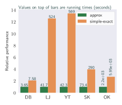
Figure 1: Relative performance of the approximate and simple-exact average-linkage algorithms on real-world graphs from the SNAP datasets, normalized to the fastest time per graph. The value on top of each bar is the running time in seconds.

5.1 Experiments

Approximate vs. Simple-Exact Algorithm. We start by evaluating the performance of our near-linear time approximation algorithm for average-linkage vs. a simple implementation of an exact average-linkage algorithm which updates the weights of all edges incident to a newly merged cluster. We ran this experiment on a collection of large real-world graphs from the SNAP datasets. Since these graphs are originally unweighted, we set the similarity of an edge $(u,v)$ to $\frac{1}{\log(d(u)+d(v))}$. We provide more details about our graph inputs in the appendix. Figure 1 shows the result of the experiment. Our approximate average-linkage algorithm (using $\epsilon=0.1$) achieves an average speedup of 6.9x over the exact average-linkage algorithm. We note that the dendrograms in the cases where the simple-exact algorithm performs reasonably well are shallower than in cases where the algorithm performs poorly (e.g., the DB dendrogram is 99x shallower than that of YT, although the number of vertices in DB is only 2.6x smaller). A simple upper-bound for the time-complexity of the simple-exact algorithm is $O(nD)$ where $D$ is the depth of the dendrogram. For other linkage measures, such as single-, complete-, and WPGMA-linkage, we achieve up to 730x speedup over the simple-exact algorithm that spends $O(d(u)+d(v))$ time to merge two clusters, and note that the dendrograms observed for these measures have very high depth.

Comparison with Metric Clustering. Next, we study the quality and scalability of our graph-based HAC algorithms compared to metric HAC algorithms. Given an input pointset, $P$, we first apply an approximate $k$-NN algorithm to $P$ to build an approximate $k$-NN graph. We use the state-of-the-art ScaNN $k$-NN library [22] for this graph-building step. We note that ScaNN internally uses multithreading, which we did not disable. We then symmetrize the $k$-NN graph and run our graph-based HAC implementation on it. We compare our results with those of the widely-used Scikit-learn (sklearn) package.

Quality. In the first set of experiments, we evaluate our algorithms and the four HAC variants supported by sklearn on the iris, wine, digits, and cancer, and faces classification datasets. We note that the heap-based and chain-based algorithms yielded the same dendrograms. To measure quality, we use the Adjusted Rand-Index (ARI) and Normalized Mutual Information (NMI) scores. The level of the tree with the highest score is used for evaluation.

We show the full quality scores in the appendix. Overall, our graph-based algorithms produce results that are comparable with, and sometimes superior to the results of the metric-based algorithms in sklearn. One exception is our complete-linkage algorithm, which is almost always worse than the sklearn algorithm, which is because the $k$-NN graph is missing large-distance edges which prevent cluster formation in the metric setting. We note that running our complete-linkage algorithm on the complete graph (with all distance edges) results in clustering results that match the quality of the sklearn algorithm. Our simple-exact and approximate average-linkage algorithm (using $\epsilon=0.1$) achieve essentially the same quality results as the exact sklearn algorithm (our algorithms achieve on average 1.8% better ARI and 0.5% better NMI). Furthermore, the approximate and simple-exact algorithms yield identical quality results for all but the digits dataset, where the simple-exact algorithm is less than 1% better for both quality measures.

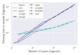
Figure 2: End-to-end running times of the sklearn and our graph-based algorithms on varying-size slices of the Fashion dataset.

Scalability. In the second set of experiments, we study whether our approach can yield end-to-end speedups over the sklearn algorithms on large pointsets. We use the Fashion-MNIST (764-dimensions), Last.fm (65 dimensions), and NYTimes (256 dimensions) datasets in these experiments. We run both the sklearn and our algorithms on slices of these datasets to understand how the running time scales as the number of points to cluster increases.

Our results for the Fashion-MNIST dataset (shown in Figure 2) show that after about 10000 points, the end-to-end time of using the graph-based approach is always faster than using the $O(n^{2})$ time metric-based algorithm. For the full Fashion-MNIST dataset, which contains 60,000 points, our approach yields an overall speedup of 20.7x.

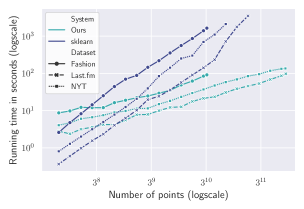
Figure 3: End-to-end running times of sklearn’s average-linkage and graph-based approximate average-linkage on varying-size slices of the Last.fm and NYTimes datasets.

In Figure 3 we show the results of the same experiment using the Last.fm and NYTimes datasets, but using only our approximate average-linkage algorithm to reduce clutter (this is the slowest algorithm out of all of our linkage-measures). We terminated algorithms that ran for longer than 1 hour, and were therefore unable to finish running the metric-based algorithm on the full Last.fm (292,385 points) and NYTimes (290,000 points) datasets. Our algorithms achieve up to 36.2x speedup on the NYTimes dataset and 76.5x speedup on the Last.fm dataset over the available datapoints for sklearn. Extrapolating from the trends of the sklearn implementations, a rough estimate suggests speedups of between 200x–500x for these datasets.

We note that we also ran the same experiments with the C++-based HAC implementations provided in SciPy [40] a nd Fastcluster [32]. We obtained running times that were within 10% of the running times of sklearn for all of our datasets and linkage functions, and thus only report the running times for sklearn in Figures 2 and 3.

Limits of our Approach. We observed that once we have generated a graph input, our algorithm’s performance scales almost linearly with the number of edges in the graph. Currently, the main bottleneck in our experiments for pointsets is the graph-building step which generates the $k$-NN graph using ScaNN and writes the $k$-NN graph to disk. Supplying the generated $k$-NN graph to our HAC algorithms without first writing it to disk will further accelerate our algorithms.

Ignoring the cost of the writing to disk, both the memory usage and running time of the graph-clustering step is lower than that of ScaNN. Specifically, the memory usage of our algorithms (excluding ScaNN) is approximately $56\cdot m+O(n)$ bytes (where the constant on the $n$ term is small). Therefore, our implementations can solve graphs with up to several billion vertices and 2–3 billion edges on a machine with 256GB of memory (obtainable from Google Cloud for a few dollars per hour). In terms of running time, we observed that our graph-based algorithms scale linearly with the number of edges in practice, and we could thus solve such a graph in between 12–24 hours.

6 Conclusion

In this paper we designed efficient HAC algorithms which run in near-linear time with respect to the number of input similarity pairs. We conducted a preliminary empirical evaluation, which shows that our algorithms achieve significant speedups while maintaining competitive clustering quality.

For future work, it would be very interesting to understand the parallel complexity of graph-based HAC, and to design efficient exact and approximate algorithms for these problems in a parallel or dynamic setting. From an experimental perspective, a significant challenge is to design HAC implementations that can be run on graphs with tens of billions of edges in a reasonable amount of time. Combining the ideas in this paper with an efficient dynamic graph processing system such as Aspen [15] may be a first step towards such a result. Finally, an interesting open question is to design a near-linear time exact HAC algorithm for the unweighted average-linkage measure.

Appendix A Algorithms and Definitions

For ease of reference, we restate a few keys definitions and algorithms that are used in the rest of the appendix.

A.1 Linkage Measures

Let the best-neighbor of a cluster $X$ be $\operatorname*{arg\,max}_{Y\in N(X)}\mathcal{W}(X,Y)$. We call the edge connecting $X$ and its best-neighbor $Y$ the best-edge of $X$. We say that a linkage measure is reducible [4], if for any three clusters $X,Y,Z$ where $X$ and $Y$ are mutual best-neighbors, it holds that $\mathcal{W}(X\cup Y,Z)\geq\max(\mathcal{W}(X,Z),\mathcal{W}(Y,Z))$. Our framework yields exact HAC algorithms for any reducible linkage measure that also satisfies the following property.

Definition A.1.

A linkage measure is called triangle-based if it satisfies the following property. Consider any step of the algorithm which merges clusters $B$ and $C$ into a cluster $B\cup C$. Let $A$ be a cluster distinct from $B$ and $C$. Then, if edge $(A,C)$ does not exist, $\mathcal{W}(A,B)=\mathcal{W}(A,B\cup C)$.

A.2 Algorithms

Most of our algorithms use the Merge routine to merge two clusters, which is given in Algorithm 1. We provide the two main HAC implementations in our framework, which are based on the classic nearest-neighbor chain and heap-based methods (Algorithm 2 and Algorithm 3 respectively).

Appendix B Neighbor-Heap Details

Augmented Heaps. A simple implementation of neighbor-heaps is to store the edges incident to a cluster using an augmented binary tree, or an augmented heap. Given a binary tree storing key-value entries, and a function $f$ taking an entry and yielding a real-valued priority, we can obtain a max-heap (min-heap) by setting the initial augmented value of each vertex to its priority calculated using $f$, and inductively setting the augmented values for internal vertices using $\max$ ($\min$) of their augmented value, and the augmented values of their two children. We refer to [39] for details on implementing augmented binary trees.

The BestEdge operation can be implemented by having the augmented value at each tree vertex (corresponding to an edge of the graph) be the edge weight, and the augmentation function to $\max$. Extracting the best-edge can then be done using a find-like function which finds a (key, value) pair in the tree that exhibits the overall augmented value of the tree. Another way is to set the augmented value to a pair of the edge weight and the neighbor id, and have the augmentation function to take a lexicographic maximum. The best-edge in this approach is simply the augmented value at the root of the tree. In our implementations, we use the former approach, since it is more space-efficient than the latter approach. Both implementations cost $O(\log n)$ work per BestEdge operation.

The Union operation can be implemented by using Union on the underlying augmented binary trees. The algorithm from [5] (which is implemented in the PAM library [39]) merges two trees of size $n,m$ with $n\leq m$ in $O(n\log(m/n+1))$ time, which is asymptotically optimal for comparison based algorithms [6].

Appendix C Deferred Proofs

Lemma C.1.

Single-linkage, complete-linkage, and WPGMA-linkage are all triangle-based linkages.

Proof.

It is well known that all of these linkage rules are reducible (e.g., see  [28]). To show that they also satisfy Definition A.1, observe that the weight of an edge $(A,B)$ can change after merging clusters $B$ and $C$ only when $A$ is also connected to $C$. For example, for single-linkage, it is easy to see that the edges that we take the $\max$ over when calculating $\mathcal{W}(A,B\cup C)=\max_{(x,y)\in E(A,B\cup C)}w(x,y)$ can affect the result only when $\mathcal{W}(A,C)>\mathcal{W}(A,B)$. Similar calculations show that complete-linkage and WPGMA-linkage are triangle-based linkages. ∎

C.1 Framework Analysis

Lemma C.2.

Let $m_{1},\ldots,m_{n-1}$ be the sequence of merge operations performed by an algorithm where $m_{i}=(u_{i},v_{i})$. Let $\mathsf{Cost}(m_{i})=\min(d(u_{i}),d(v_{i}))$, where $d(u_{i})$ and $d(v_{i})$ are the degrees of the clusters when they are merged. Then, the total cost $\sum_{i=1}^{n-1}\mathsf{Cost}(m_{i})=O(m\log n)$.

Proof.

The proof is by a charging argument. Following the definition of $\mathsf{Cost}$, assign a token to each edge in $N(\operatorname*{arg\,min}(d(u_{i}),d(v_{i})))$ for each $i$. We do not undercount the cost, since we assign $\mathsf{Cost}(m_{i})$ tokens at each step $i$ to the edges. We now bound the total cost by bounding the number of tokens that can be assigned to an edge.

We conceptually add an extra total-edges variable, $\mathcal{T}(u)$ to the data structures storing the vertex neighborhoods, $N(u)$. This variable simply stores the total number of edges that have been merged into this tree. At the start of the algorithm, $\mathcal{T}(u)=d(u)$. When two clusters $u$ and $v$ merge, if $v$ is the cluster remaining active after the merge, $\mathcal{T}(v)$ is incremented by $\mathcal{T}(u)$. Let $A$ be the set of active clusters. It is easy to check that $\sum_{c\in A}\mathcal{T}(c)=2m$ at all points in the algorithm.

Next, we bound the maximum number of tokens assigned to an edge by observing that each time an edge has a token assigned to it in some step $i$, the total-edges of the set containing it doubles. Since $\mathcal{T}(u)$ of a set $u$ can grow to at most $2m$, each edge can receive at most $O(\log m)=O(\log n)$ tokens, and thus the total cost is $O(m\log n)$. ∎

Theorem 5.

There are deterministic implementations of the chain-based and heap-based algorithms that run in $O(m\log^{2}n)$ time for any triangle-based linkage $\mathcal{L}$.

Proof.

We first bound the time-complexity for the merge steps that both algorithms have in common. Both algorithms perform $n-1$ merge operations, whose total cost is $O(m\log n)$ using Lemma C.2. To translate this cost measure back to time-complexity, we note that the total time taken for the $i$-th merge step using the deterministic neighbor-heap implementation is at most $O(\mathsf{Cost}(m_{i})\log(n/\mathsf{Cost}(m_{i})+1))=O(\mathsf{Cost}(m_{i})\log n)$, and thus the total time to perform all merges is $O(m\log^{2}n)$. We bound the time of the remaining algorithm-specific steps separately.

Chain-based Algorithm. We use a few well-known facts about this algorithm, namely that (i) each of the $2n-1$ clusters that appears in the dendrogram is pushed onto the stack exactly once, and (ii) the number of times BestEdge is called is $O(n)$. Therefore, the total time-complexity of these steps is $O(n\log n)$ and the overall time-complexity is $O(m\log^{2}n)$.

Heap-based Algorithm. The remaining steps involve extracting edges from the global heap $H$. We analyze two types of edges that can be extracted: (i) edges whose remaining endpoint is inactive and (ii) edges whose remaining endpoint is active. There are at most $n-1$ type (ii) edges, since each type (ii) edge results in a merge, and so the time spent processing these edges is $O(n\log n)$. Next, for the type (i) edges, observe that each such edge can be charged to the deactivated endpoint, $v$, and that the total number of charges for a cluster $v$ is at most its degree at the time it was deactivated. Thus, the total cost for these edges is $\sum_{i=1}^{n-1}\mathsf{Cost}(m_{i})=O(m\log n)$ (by Lemma C.2) and the time-complexity for these steps is $O(m\log^{2}n)$ since each inactive edge takes $O(\log n)$ time to extract the current best edge from its active endpoint, and to update $H$. Thus, the overall time-complexity is $O(m\log^{2}n)$. ∎

C.2 A Faster Randomized Chain-Based Algorithm

In this section we present a randomized implementation of our chain-based algorithm which runs in $O(m\log n)$ time.

Overview. There are two challenges posed by Algorithm 1 that we must implement more efficiently in order to achieve an $O(m\log n)$ time HAC algorithm.

1. The merge-cost from Lemma C.2 is $O(m\log n)$. Thus, in order to achieve $O(m\log n)$ time we must perform each merge operation in (amortized) $O(1)$ time per merged element.

2. The overall algorithm also performs $O(m\log n)$ neighbor-updates in Line 7 of Algorithm 1, which remove the id of a merged vertex from an active neighbor’s neighbor-heap and relabel it to the id of the new neighbor. Thus, we must either handle these updates lazily, or also handle them in (amortized) $O(1)$ time per operation.

Our approach to handle (1) is to use a faster randomized implementation of neighbor-heaps which we outline below. The high-level idea is to use an efficient meldable heap, such as a Fibonacci heap or Leftist heap in conjunction with hash tables. We deal with (2) by eagerly updating the hash tables of our neighbors when performing a merge, but lazily updating the IDs stored in the meldable heap, except when we identify an edge that is being merged. The overall cost of the hash table updates is $O(m\log n)$ time in expectation. Although the updates to the heaps cost $O(\log n)$ time each, since they require deleting two existing elements and reinserting a new merged element, each of these updates can be assigned uniquely to an edge in the original graph, and thus the overall time complexity for these updates is also $O(m\log n)$. We now provide a detailed description of our approach.

C.2.1 Neighbor-Heaps using Meldable Heaps and Hashing

We give an alternative implementation of neighbor-heaps, which is asymptotically faster than the augmented-heap based implementation at the cost of using randomization. The idea is to use a heap data structure that supports efficient melding, such as Fibonacci heaps [18], in combination with a hash table. The neighbor-heap representation for a cluster $v$ is a pair of a heap and a hash-table where the neighbors of $v$ are stored in both data structures. Let $\mathcal{H}(A)$ denote the heap and $\mathcal{Q}(A)$ denote the table for a cluster $A$. The elements in $\mathcal{H}(A)$ are pairs of a cluster-id, $C$, and the associated weight of this edge $\mathcal{W}(A,C)$. The priority of an element is just the weight. The elements in $\mathcal{Q}(A)$ are triples of a key (a cluster-id), $C$, the associated weight of this edge $\mathcal{W}(A,C)$, and a pointer to the location of the element for $C$ in $\mathcal{H}(A)$.

The Meld operation on two mergeable heaps $\mathcal{H}_{1},\mathcal{H}_{2}$ can be done in $O(1)$ time. Note that this operation does not detect elements in $\textsc{Keys}(\mathcal{H}_{1})\cap\textsc{Keys}(\mathcal{H}_{2})$, which is why we also store the elements in both heaps in a hash-table (which implements intersection efficiently).

We also define a T-Merge operation on two hash-tables in neighbor-heaps, $\mathcal{Q}(A)$, $\mathcal{Q}(B)$, which works as follows. Without loss of generality let $|\mathcal{Q}(A)|\leq|\mathcal{Q}(B)|$. We map over the elements in $\mathcal{Q}(A)$, and insert them into the larger size table. If an key $C$ appears in both tables, then we merge this edge using the linkage function $\mathcal{L}$. We also append $C$ and the locations of $C$ in both heaps to an array $O$ that collects all of the locations for $C\in\mathcal{Q}(A)\cap\mathcal{Q}(B)$. The T-Merge operation returns $O$ and $\mathcal{Q}(B)$. T-Merge on two tables $\mathcal{Q}(A)$, $\mathcal{Q}(B)$ runs in $O(\min(|\mathcal{Q}(A)|,|\mathcal{Q}(A)|))$ expected time.

C.2.2 Merging Clusters

Next, we present how two clusters are merged using the randomized neighbor-heap (Algorithm 6).

Algorithm 6 $\textsc{FastMerge}(A,B,\mathcal{L})$

1:Active clusters $A$ and $B$, triangle-based linkage $\mathcal{L}$.

2:Cluster id of the remaining active cluster.

3:$(A,B)=(\operatorname*{arg\,min}(d(A),d(B)),\operatorname*{arg\,max}(d(A),d(B)))$

4:Remove $B$ from $\mathcal{H}(A)$ and $\mathcal{Q}(A)$ (and vice versa).

5:$(O,\mathcal{Q}(B))=\textsc{T-Merge}(\mathcal{Q}(A),\mathcal{Q}(B))$ $\triangleright$ $O$ holds heap-locations for $C\in\mathcal{Q}(A)\cap\mathcal{Q}(B)$

6:for each $(C,L_{A},L_{B})\in O$ do

7:     Delete $C$ from $\mathcal{H}(A)$ and $\mathcal{H}(B)$ using $L_{A}$ and $L_{B}$ to find these elements.

8:     Insert $C$ into $\mathcal{H}(B)$ with the weight merged using $\mathcal{L}$. Let the pointer to this element be $L^{\prime}$.

9:     Update the location of $C$ in $\mathcal{Q}(B)$ to $L^{\prime}$.

10:$\mathcal{H}(B)=\textsc{Meld}(\mathcal{H}(A),\mathcal{H}(B))$. $\triangleright$ Before the meld, $\textsc{Keys}(\mathcal{H}(A))\cap\textsc{Keys}(\mathcal{H}(B))=\emptyset$.

11:for $C\in\textsc{Keys}(\mathcal{Q}(A))$ do

12:     Update cluster-id from $A$ to $B$ in $\mathcal{Q}(C)$ and $\mathcal{H}(C)$. If $B\in\mathcal{Q}(C)$, use $\mathcal{L}$ to merge the edge weights and update both $\mathcal{Q}(C)$ and $\mathcal{H}(C)$.

13:Mark cluster $A$ as inactive.

14:Return $B$.

Algorithm 6 is similar to our original Merge algorithm, Algorithm 1 with a few key differences. First, Line 4 removes the IDs of the merged clusters from both the heaps and hash-tables for each of the merging clusters. Next, on Line 5 the algorithm merges the hash-tables of both clusters using the T-Merge routine described above. The result is a sequence $O$ of triples containing the cluster-id, and two heap-locations of $C\in\textsc{Keys}(\mathcal{Q}(A))\cap\textsc{Keys}(\mathcal{Q}(B))$, and the newly merged table, $\mathcal{Q}(B)$. The algorithm then loops over these clusters $C$ with edges to both $A$ and $B$, and the location of these edges in $\mathcal{H}(A)$ and $\mathcal{H}(B)$ (Lines 6–9). For each such cluster, the algorithm first deletes $C$ from $\mathcal{H}(A)$ and $\mathcal{H}(B)$ using the given locations (Line 7). It then inserts $C$ into $\mathcal{H}(B)$ with the updated weight of this edge (Line 8). Note that at this point, $\textsc{Keys}(\mathcal{H}(A))\cap\textsc{Keys}(\mathcal{H}(A))=\emptyset$. After the loop, the algorithm first melds the two heaps (Line 10). The last step is to update the neighbor-heaps of neighbors of $A$ (the deactivated cluster). The algorithm iterates over all neighbors $C$ of $A$ on Line 11, and on Line 12, updates the id from $A$ to $B$ in $\mathcal{Q}(C)$ and $\mathcal{H}(C)$. Note that the location of $A$ in $\mathcal{H}(C)$ is stored $\mathcal{Q}(C)$. If $C$ also has an edge to $B$, it sets the weight of the $(C,B)$ edge to the updated weight in $\mathcal{Q}(C)$. It also deletes $A$ and $B$ from $\mathcal{H}(C)$ and reinserts $B$ into $\mathcal{H}(C)$ with the correct weight. Finally, it marks $A$ as inactive and returns the ID of the remaining active cluster, $B$.

C.2.3 Modifications to the Chain-Based Algorithm

Lastly, we discuss how to modify the chain-based algorithm to obtain an $O(m\log n)$ time HAC for triangle-based linkage. The algorithm is identical to Algorithm 2 with the only differences being the representation of the neighbor-heap data structures, and the merge routine. Specifically, the call to Merge on Line 11 uses the FastMerge algorithm (Algorithm 6). As Lemma C.3 shows, after a merge, the state of the neighbor-heap data structures corresponds to the state of the current graph induced by the active clusters, and thus we do not have to modify BestEdge.

Lemma C.3.

After a call to Algorithm 6, the adjacency information stored in the neighbor-heaps (both $\mathcal{H}(A)$ and $\mathcal{Q}(A)$) of all active clusters $A$ is correct.

Proof.

The proof is by induction. Consider the $k$-th merge between two vertices $A$ and $B$, and assume that the claim holds before this merge. Assume without loss of generality that $A$ is deactivated and $B$ remains active. The only clusters affected by the merge are $\{B\}\cup\{C\in N(A)\}$, since all neighbors in $N(B)\setminus N(A)$ have an edge to $B$ with the same weight as before the merge.

First, we show that Algorithm 6 correctly updates the edges incident to $B$. The only edges that experience weight change are those in $N(A)\cap N(B)$, which the algorithm detects when performing T-Merge on Line 5. For each neighbor $C$ in $N(A)\cap N(B)$, it deletes $C$ from both $\mathcal{H}(A)$ and $\mathcal{H}(B)$ (Line 7) and reinserts $C$ into $\mathcal{H}(B)$ with the correct weight. Finally, the location corresponding to $C$ is updated in $\mathcal{Q}(B)$. Note that T-Merge also sets the weight of $C$ correctly in $\mathcal{Q}(B)$. The remaining affected edges are new neighbors of $B$, which are correctly labeled and stored in $\mathcal{Q}(B)$ and $\mathcal{H}(B)$.

Second, we show that Algorithm 6 correctly updates the neighbor-heaps for $C\in N(A)$. It processes these neighbors in the for-loop on Line 11. If the neighbor $C$ is not in $N(A)\cap N(B)$, it just updates the cluster-id from $A$ to $B$ in $\mathcal{H}(C)$, and leaves the location in $\mathcal{Q}(C)$ unchanged. Otherwise, for $C\in N(A)\cap N(B)$, it deletes $A$ and $B$ from $\mathcal{H}(C)$, updates the weight of the edge using $\mathcal{L}$ and reinserts $B$ into $\mathcal{H}(C)$ (similarly for $\mathcal{Q}(C)$). Therefore, all of the neighbors $C\in N(A)$ reference $B$ after Algorithm 6 finishes. ∎

Using Lemma C.3 we have that the state of the neighbor-heap data structures correspond to the current state of the graph induced by the active clusters after performing a merge operation. Combining the fact that the neighbor-heap data is always correct after a merge with the existing proof for the correctness of the chain-based algorithm suffices to show that our randomized implementation is correct. Next, we show that our approach is also efficient.

Theorem 6.

There is a randomized implementation of the chain-based algorithm that runs in $O(m\log n)$ time in expectation for any triangle-based linkage $\mathcal{L}$.

Proof.

We follow the proof of Theorem 5 and separately account for the cost of the merge steps, and the cost of the remaining steps in the algorithm.

The algorithm performs $n-1$ merge operations, with a total merge-cost of $O(m\log n)$ using Lemma C.2. To translate this cost measure to the time-complexity measure, we examine the two types of operations done inside of the FastMerge algorithm (Algorithm 6).

The first type of updates are those done on the hash-tables, $\mathcal{Q}(C)$ for a cluster $C$. Over all merges, there are $O(m\log n)$ such operations, which each cost $O(1)$ time in expectation, and thus the overall cost of the hash-table updates are $O(m\log n)$ in expectation.

The second type of updates are done on the heaps. First, the cost of melding the two heaps is $O(1)$ amortized using lazy Fibonacci heaps and $O(\log n)$ using Leftist or eager Fibonacci heaps. In either case, the overall cost of the meld operations is at most $O(n\log n)$. The remaining heap operations can be broken up further into two categories of heap updates which update the cluster-ids and weights of edges in the heaps.

1. Updates that only affect the cluster-ids of an edge cost $O(1)$ time each in expectation, since they are done by looking up the location of the edge in the hash-table, and updating the id of this element in $O(1)$ time.

2. Updates that change the weights of edges in the heap are more costly since they require deleting and reinserting elements from the heap, and deleting an element costs $O(\log n)$ time. However, updating the weight of an edge is done only when two clusters $A,B$ merge and both $A,B$ have an edge to a neighbor cluster $C$. We observe that we can charge the cost of this step to one of the original edges in the graph, and that each original edge is charged at most once.

For heap updates of type (1), the cost is thus $O(m\log n)$ time in expectation. For heap updates of type (2), there are at most $O(m)$ of these updates, and each costs $O(\log n)$ time for a total cost of $O(m\log n)$ time.

Finally, the remaining steps in the algorithm outside of the merge steps are $O(n)$ BestEdge queries, which each cost $O(\log n)$ time for a total cost of $O(n\log n)$ time. Thus, the overall time-complexity of the algorithm is $O(m\log n)$ in expectation, as desired.

∎

C.3 Exact Unweighted Average-Linkage

First, we present again the two key subroutines that make up our exact unweighted average-linkage algorithm (Algorithms 7 and Algorithm 8).

Algorithm 7 $\textsc{FlipEdge}(A,B)$

1:Edge oriented from active clusters $A$ to $B$.

2:Edge oriented from $B$ to $A$.

3:$w=\mathcal{W}(A,B)$. [true weight of the edge]

4:Update the edge $(A,B,w)$ in $\textsc{Heap}(A)$.

Algorithm 8 $\textsc{UpdateOrientation}(A,B,\mathcal{EO})$

1:Active clusters $A$ and $B$, dynamic orientation structure $\mathcal{EO}$.

2:$(A,B)=(\operatorname*{arg\,min}(d(A),d(B)),\operatorname*{arg\,max}(d(A),d(B))$.

3:For each $C\in N(A)$, delete $(C,A)$ and insert $(C,B)$ into the orientation data structure. Edge flips are handled using FlipEdge [Algorithm 7]

4:for each edge $(B,C)$ oriented out of $B$ do

5:     $w=\mathcal{W}(B,C)$. [true weight of the edge]

6:     Update the edge $(B,C,w)$ in $\textsc{Heap}(C)$.

Let $\hat{G}$ denote the directed graph induced by the active clusters, with edges oriented according to the edge-orientation $\mathcal{EO}$. We start by proving a lemma that helps prove that our exact unweighted average-linkage algorithm is correct.

Lemma C.4.

After a call to Algorithm 1, for each active cluster $A$, the weights of all edges directed towards $A$ in $\hat{G}$ are set correctly in $\textsc{Heap}(A)$.

Proof.

The proof is by induction. Consider the $k$-th merge between two clusters $A$ and $B$, and assume that the claim holds before this merge. Assume without loss of generality that $A$ is deactivated by this merge, and $B$ remains active. Recall that the merge algorithm will also invoke Algorithm 8, which updates the orientation by remapping edges that are incident to the deactivated cluster from the maintained orientation $\mathcal{EO}$, and that Algorithm 7 is invoked each time the dynamic edge-orientation algorithm flips an edge.

For any edges that are flipped during the execution of Algorithm 8, the weights of these edges are correctly set in the heap of the cluster that the edge now points to (the head of this edge). The reason is that Algorithm 7 is invoked upon each edge flip and this algorithm computes the correct weight of the edge and updates the weight in the heap of the head of this edge. This accounts for all edges that are flipped by the orientation algorithm when deleting all $(A,C)$ (undirected) edges and reinserting them as $(B,C)$ edges.

The only remaining edges which may not have updated their out-neighbors are new edges incident to $B$ that are oriented out of $B$. Thus, Algorithm 8 maps over all edges oriented out of $B$ and sets the weight of these edges correctly in the heap of the head of this edge.

We have accounted for (i) all edges whose orientation flips due to the deletions and insertions in the merge and (ii) the new edges oriented out of $B$. Finally, by assumption, the remaining edges have their correct weights set in the heaps of the head of these edges, and thus all active clusters $A$ have the correct weights for edges that point to them. ∎

Theorem 7.

The exact average-linkage algorithm is correct and runs in $\tilde{O}(n\sqrt{m})$ time for arbitrary graphs.

Proof.

To show correctness, by Lemma C.4, we have that after the $i$-th merge, the state of each active cluster’s heap is correct for all but the $O(\alpha_{i})$ edges that are oriented out of this cluster. Since before performing a BestEdge computation, the algorithm maps over all $O(\alpha_{i})$ of these edges and updates the weight of these edges in its heap to the correct weight, all of the edges in its heap have the correct weight, and thus the cluster selects the best-edge incident to it. The correctness of the overall algorithm can now by obtained by combining this proof with the existing proof for the correctness of the nearest-neighbor chain algorithm.

Next, we analyze the time-complexity of our algorithm. We first bound the extra cost incurred by maintaining the dynamic graph-orientation data structure $\mathcal{EO}$ over the course of the algorithm. Using the dynamic graph-orientation data structure of Henzinger et al. [23], we obtain an amortized cost of $O(\log^{2}n)$ for each edge insertion and deletion. The dynamic graph-orientation data structure is only updated and used during the $\textsc{Merge}()$ and $\textsc{BestEdge}()$ operations. Consider the $i$-th such operation, and let $G_{i}$ be the graph induced by the current clustering at the time of this operation.

Using Lemma C.2, the total number of merge operations is at most $O(m\log n)$. For each of these operations, we have to perform an edge insertion and deletion, which could translate to a total $O(m\log^{3}n)$ edge flips. Each edge flip also requires $O(\log n)$ time to update the weight of the edge in the heap of the new head of this edge. Thus the total cost of the edge insertions, deletions, and flips is $O(m\log^{4}n)$ over the course of the entire algorithm.

The merge algorithm also processes the edges incident to the remaining active cluster, $B$. The cost for this step is $O(\alpha_{i}\log n)$, since there are $O(\alpha_{i})$ edges oriented out of $B$ and we pay $O(\log n)$ to perform a heap-update for each one. Since there are $n-1$ merges, the overall cost for this step is $O(\log n\sum_{i=1}^{n-1}\alpha_{i})$ over the course of the entire algorithm.

Lastly, the cost for performing the BestEdge operation is $O(\alpha^{*}_{i})$ where $\alpha^{*}_{i}$ is the current arboricity at the time of the $i$-th BestEdge operation. Note that there may be many BestEdge operations performed before a merge is performed. Since there are $2n-2$ BestEdge operations, the overall cost is $O(\sum_{i=1}^{2n-2}\alpha^{*}_{i})$.

By bounding each $\alpha_{i},1\leq i\leq n-1$ and $\alpha^{*}_{j},1\leq j\leq 2n-2$ above as $\alpha_{\max}\leq\sqrt{m}$, the maximum arboricity of the graph over the entire sequence of merges, the overall time-complexity of the algorithm is

$$O(m\log^{4}n+n\log n\cdot\alpha_{\max})=\tilde{O}(n\sqrt{m}).$$

∎

C.4 Approximate Unweighted Average-Linkage

We start by recalling the notion of approximation and the invariant used in our approximation algorithm. An $\epsilon$-close HAC algorithm is an algorithm which only merges edges that have similarity at least $(1-\epsilon)\cdot\mathcal{W}_{\max}$ where $\mathcal{W}_{\max}$ is the largest weight currently in the graph [29].

The idea of our algorithm is to maintain an extra counter for each cluster which stores the size the cluster had at the last time that the algorithm updated all of the incident edges of the cluster. Call this variable the staleness, $\mathcal{S}(A)$, of a given cluster $A$. Recall that the size of a cluster $|A|$ is defined to be the number of initial (singleton) clusters that it contains. Our algorithm maintains the following invariant:

Invariant 2.

For any active cluster $A$, $|A|<(1+\epsilon)\mathcal{S}(A)$.

Let the stored similarity of an edge $(u,v)$ in the neighborhood be denoted $W_{\mathcal{S}}(u,v)$ and the true similarity of this edge be $W_{\mathcal{T}}(u,v)$. The next lemma bounds the maximum error an algorithm maintaining Invariant 2 can observe for an edge incident to an active cluster.

Lemma C.5.

Let $e=(U,V)$ be an edge in the neighborhood of an active cluster $U$. Then, $(1+\epsilon)^{-2}W_{\mathcal{S}}(U,V)\leq W_{\mathcal{T}}(U,V).$

Proof.

There are two ways that the similarity of the $(U,V)$ edge can change as the algorithm merges clusters:

1. By a merge which adds parallel edges to $\mathsf{Cut}(U,V)$ (e.g., if $U$ merges with a cluster $Z$ which is also connected to $V$, thereby increasing the total similarity of edges crossing the cut).

2. By a merge to $|U|$ or $|V|$ that does not affect the total similarity of edges going across $\mathsf{Cut}(U,V)$ (e.g., if $U$ merges with a cluster $Z$ that is not connected to $V$).

If a Type 1 update occurs, then the similarity of this edge will be set to the true value upon this update, since the algorithm will update the similarities of every edge in the intersection of the merge. Therefore, we can ignore these updates when trying to bound the maximum drift between the true and stored similarities. On the other hand, we could have many Type 2 updates occur. In this case, the similarity of this edge will not be updated unless Invariant 2 becomes violated for either $U$ or $V$. Therefore, we have the following upper bounds on the maximum size of $U$ and $V$, namely that $|U|<(1+\epsilon)S(U)$ and $|V|<(1+\epsilon)S(V)$.

In the worst case, the stored similarity could have used $S(U)$ and $S(V)$ to normalize (since the similarity must have been updated when these stored similarities were set), and the true similarity could use $(1+\epsilon)S(U)$ and $(1+\epsilon)S(V)$. Since the sum term in the similarity equation doesn’t change (since there are no Type 1 updates), we have that

$$W_{\mathcal{S}}(U,V)\leq\frac{1}{S(U)\cdot S(V)}\cdot\sum_{(u,v)\in\mathsf{Cut}(U,V)}w(u,v)$$

and therefore

$$W_{\mathcal{T}}(U,V)\geq\frac{1}{(1+\epsilon)^{2}\cdot S(U)\cdot S(V)}\cdot\sum_{(u,v)\in\mathsf{Cut}(U,V)}$$

Therefore, the true similarity is at most a $(1+\epsilon)^{-2}$ factor smaller than the stored similarity. ∎

Theorem 8.

There is an $\epsilon$-close HAC algorithm for the average-linkage measure that runs in $O(m\log^{2}n)$ time.

Proof.

First we show that our algorithm is $\epsilon$-close. Let $\delta$ be the closeness parameter used internally in the algorithm, which we will set shortly. For each $(U,V)$ edge, since the simialrities in the algorithm only decrease, we have that $W_{\mathcal{T}}(U,V)\leq W_{\mathcal{S}}(U,V)$. Combining this fact with Lemma C.5, we have that

$$(1+\delta)^{-2}W_{\mathcal{S}}(U,V)\leq W_{\mathcal{T}}(U,V)\leq W_{\mathcal{S}}(U,V)$$

for all active edges $U,V$.

Next, consider a merge step in the algorithm which merges two clusters $A,B$. We have that $W_{\mathcal{S}}(A,B)$ is the largest stored similarity among any active cluster in the graph. We also have that $(1+\delta)^{-2}W_{\mathcal{S}}(A,B)\leq W_{\max}$ where $W_{\max}$ is the current maximum similarity in the graph, since otherwise the stored similarity corresponding to $W_{\max}$ would be larger than $W_{\mathcal{S}}(A,B)$ and thus $(A,B)$ would not be the edge selected from the global heap, $H$. Therefore our approach yields a $(1-(1+\delta)^{-2})$-close algorithm, and by setting $\delta=\sqrt{1/(1-\epsilon)}-1$ we obtain an $\epsilon$-close algorithm.

Lastly, we show that the algorithm runs in $O(m\log^{2}n)$ time for any given constant $\epsilon$. Other than the extra work done to update stale clusters, the algorithm is identical to the heap-based algorithm from our framework. To bound the work done for stale clusters, observe that each cluster can become stale at most $O(\log_{1+\delta}n)=O(\log_{1+\epsilon}n)$ times, and performs $O(\log n)$ work per incident edge each time it becomes stale. Since each of the original $m$ edges is associated with at most two active clusters at any point in the algorithm, the overall time-complexity of updating stale vertices is $O(m\log_{1+\epsilon}n\log n)=O(m\log^{2}n)$ for any constant $\epsilon$. Combining this with the time-complexity of the heap-based algorithm completes the proof. ∎

Appendix D Experimental Evaluation

Graph Data. We list information about graphs used in our experiments in Table 1. com-DBLP (DB) is a co-authorship network sourced from the DBLP computer science bibliography. YouTube (YT) is a social-network formed by user-defined groups on the YouTube site. Skitter (SK) is an internet topology graph generated from traceroutes. LiveJournal (LJ) is a directed graph of the social network. com-Orkut (OK) is an undirected graph of the Orkut social network. These graphs are sourced from the SNAP dataset [27].

Another family of graphs that we consider are generated from point datasets by using an approximate $k$-NN graph construction. All of the point datasets that we use can be found in the sklearn.datasets package. We note that the large real-world graphs that we study are not weighted, and so we set the similarity of an edge $(u,v)$ to $\frac{1}{\log(d(u)+d(v))}$. We symmetrized all directed graph inputs considered in this paper.

Table 1: Graph inputs, including vertices and edges.

Graph Dataset	Num. Vertices	Num. Edges
com-DBLP (DB)	425,957	2,099,732
YouTube-Sym (YT)	1,138,499	5,980,886
Skitter-Sym (SK)	1,696,415	22,190,596
LiveJournal-Sym (LJ)	4,847,571	85,702,474
com-Orkut (OK)	3,072,627	234,370,166

Table 2: Adjusted Rand-Index (ARI) and Normalized Mutual Information (NMI) scores of our graph-based HAC implementations (columns 2–5) versus the HAC implementations from sklearn (columns 6–9). The scores are calculated by evaluating the clustering generated by each cut of the generated dendrogram to the ground-truth labels for each dataset. Our graph-based implementations run over an approximate $k$-NN graph with $k=50$.

	Dataset	Single	Complete	WPGMA	Apx-Avg	Avg	Sk-Single	Sk-Complete	Sk-Avg	Sk-Ward
ARI	iris	0.702	0.462	0.605	0.759	0.759	0.714	0.642	0.759	0.731
	wine	0.297	0.286	0.317	0.331	0.331	0.297	0.370	0.351	0.368
	digits	0.661	0.133	0.500	0.876	0.880	0.661	0.478	0.689	0.812
	cancer	0.561	0.543	0.539	0.489	0.489	0.561	0.464	0.537	0.406
	faces	0.467	0.438	0.480	0.508	0.508	0.467	0.471	0.529	0.608
NMI	iris	0.733	0.641	0.733	0.805	0.805	0.761	0.722	0.805	0.770
	wine	0.410	0.388	0.387	0.427	0.427	0.417	0.463	0.448	0.448
	digits	0.772	0.572	0.713	0.900	0.902	0.778	0.729	0.838	0.868
	cancer	0.316	0.359	0.384	0.460	0.460	0.385	0.442	0.456	0.446
	faces	0.847	0.846	0.857	0.859	0.859	0.856	0.855	0.867	0.871

References

- [1] A. Abboud, V. Cohen-Addad, and H. Houdrouge. Subquadratic high-dimensional hierarchical clustering. In Advances in Neural Information Processing Systems (NeurIPS), pages 11580–11590, 2019.
- [2] M. Bateni, S. Behnezhad, M. Derakhshan, M. Hajiaghayi, R. Kiveris, S. Lattanzi, and V. Mirrokni. Affinity clustering: Hierarchical clustering at scale. In Advances in Neural Information Processing Systems (NeurIPS), pages 6864–6874, 2017.
- [3] D. Beeferman and A. L. Berger. Agglomerative clustering of a search engine query log. In ACM SIGKDD International Conference on Knowledge Discovery and Data Mining, pages 407–416, 2000.
- [4] J.-P. Benzécri. Construction d’une classification ascendante hiérarchique par la recherche en chaîne des voisins réciproques. Cahiers de l’analyse des données, 7(2):209–218, 1982.
- [5] G. E. Blelloch, D. Ferizovic, and Y. Sun. Just join for parallel ordered sets. In ACM Symposium on Parallelism in Algorithms and Architectures (SPAA), pages 253–264, 2016.
- [6] M. R. Brown and R. E. Tarjan. A fast merging algorithm. Journal of the ACM (JACM), 26(2):211–226, 1979.
- [7] M. Charikar and V. Chatziafratis. Approximate hierarchical clustering via sparsest cut and spreading metrics. In ACM-SIAM Symposium on Discrete Algorithms (SODA), page 841–854, USA, 2017.
- [8] M. Charikar, V. Chatziafratis, and R. Niazadeh. Hierarchical Clustering better than Average-Linkage, pages 2291–2304. 2019.
- [9] N. Chiba and T. Nishizeki. Arboricity and subgraph listing algorithms. SIAM Journal on Computing, 14(1):210–223, 1985.
- [10] M. Cochez and H. Mou. Twister tries: Approximate hierarchical agglomerative clustering for average distance in linear time. In ACM SIGMOD International Conference on Management of Data, pages 505–517, 2015.
- [11] V. Cohen-Addad, V. Kanade, and F. Mallmann-Trenn. Hierarchical clustering beyond the worst-case. In Advances in Neural Information Processing Systems (NeurIPS), volume 30, pages 6201–6209. Curran Associates, Inc., 2017.
- [12] V. Cohen-Addad, V. Kanade, F. Mallmann-Trenn, and C. Mathieu. Hierarchical clustering: Objective functions and algorithms. J. ACM, 66(4), 2019.
- [13] S. Dasgupta. A cost function for similarity-based hierarchical clustering. In ACM Symposium on Theory of Computing (STOC), page 118–127, New York, NY, USA, 2016. Association for Computing Machinery.
- [14] L. Dhulipala, G. E. Blelloch, and J. Shun. Theoretically efficient parallel graph algorithms can be fast and scalable. In ACM Symposium on Parallelism in Algorithms and Architectures (SPAA), pages 293–304, 2018.
- [15] L. Dhulipala, G. E. Blelloch, and J. Shun. Low-latency graph streaming using compressed purely-functional trees. In ACM SIGPLAN Conference on Programming Language Design and Implementation (PLDI), pages 918–934, 2019.
- [16] L. Dhulipala, J. Shi, T. Tseng, G. E. Blelloch, and J. Shun. The graph based benchmark suite (GBBS). In International Workshop on Graph Data Management Experiences and Systems (GRADES) and Network Data Analytics (NDA), pages 11:1–11:8, 2020.
- [17] P. Franti, O. Virmajoki, and V. Hautamaki. Fast agglomerative clustering using a k-nearest neighbor graph. IEEE Transactions on Pattern Analysis and Machine Intelligence, 28(11):1875–1881, 2006.
- [18] M. L. Fredman and R. E. Tarjan. Fibonacci heaps and their uses in improved network optimization algorithms. J. ACM, 34(3), 1987.
- [19] S. Gilpin, B. Qian, and I. Davidson. Efficient hierarchical clustering of large high dimensional datasets. In ACM International Conference on Information and Knowledge Management, pages 1371–1380, 2013.
- [20] Gorg Sissons. Gpu-accelerated R in the cloud with teraproc cluster-as-a-service, 2015. [Online; accessed 2-February-2021].
- [21] S. Guha, R. Rastogi, and K. Shim. Rock: A robust clustering algorithm for categorical attributes. In Proceedings of the International Conference on Data Engineering, page 512, USA, 1999.
- [22] R. Guo, P. Sun, E. Lindgren, Q. Geng, D. Simcha, F. Chern, and S. Kumar. Accelerating large-scale inference with anisotropic vector quantization. In International Conference on Machine Learning (ICML), pages 3887–3896, 2020.
- [23] M. Henzinger, S. Neumann, and A. Wiese. Explicit and implicit dynamic coloring of graphs with bounded arboricity. CoRR, abs/2002.10142, 2020.
- [24] G. Karypis, E.-H. S. Han, and V. Kumar. Chameleon: Hierarchical clustering using dynamic modeling. Computer, 32(8):68–75, Aug. 1999.
- [25] B. King. Step-wise clustering procedures. Journal of the American Statistical Association, 69:86–101, 1967.
- [26] G. N. Lance and W. T. Williams. A general theory of classificatory sorting strategies 1. Hierarchical systems. Computer Journal, 9(4):373–380, Feb. 1967.
- [27] J. Leskovec and A. Krevl. SNAP Datasets: Stanford large network dataset collection, 2014.
- [28] C. D. Manning, P. Raghavan, and H. Schütze. Introduction to Information Retrieval. Cambridge University Press, 2008.
- [29] B. Moseley, K. Lu, S. Lattanzi, and T. Lavastida. A framework for parallelizing hierarchical clustering methods. In ECML PKDD 2019, 2019.
- [30] B. Moseley and J. R. Wang. Approximation bounds for hierarchical clustering: Average linkage, bisecting k-means, and local search. In Advances in Neural Information Processing Systems (NeurIPS), pages 3094–3103, 2017.
- [31] F. Murtagh. A survey of recent advances in hierarchical clustering algorithms. The computer journal, 26(4):354–359, 1983.
- [32] D. Müllner. fastcluster: Fast hierarchical, agglomerative clustering routines for R and python. Journal of Statistical Software, Articles, 53(9):1–18, 2013.
- [33] N. Robertson and P. D. Seymour. Graph minors II. Algorithmic aspects of tree-width. J. Algorithms, 7(3):309–322, 1986.
- [34] A. Roy and S. Pokutta. Hierarchical clustering via spreading metrics. In Advances in Neural Information Processing Systems (NeurIPS), volume 29, pages 2316–2324. Curran Associates, Inc., 2016.
- [35] SAS Institute Inc. The CLUSTER procedure, 2020. [Online; accessed 2-February-2021].
- [36] J. Shao, S. W. Tanner, N. Thompson, and T. E. Cheatham. Clustering molecular dynamics trajectories: 1. characterizing the performance of different clustering algorithms. Journal of Chemical Theory and Computation, 3(6):2312–2334, 2007.
- [37] M. H. Smid. The well-separated pair decomposition and its applications., 2018.
- [38] P. H. Sneath and R. R. Sokal. Numerical Taxonomy: The Principles and Practice of Numerical Classification. W.H. Freeman, San Francisco, 1973.
- [39] Y. Sun, D. Ferizovic, and G. E. Blelloch. Pam: Parallel augmented maps. In ACM Symposium on Principles and Practice of Parallel Programming (PPoPP), 2018.
- [40] The SciPy community. scipy.cluster.hierarchy.linkage, 2020. [Online; accessed 2-February-2021].
- [41] J. H. Ward. Hierarchical grouping to optimize an objective function. Journal of the American Statistical Association, 58(301):236–244, 1963.
- [42] Wikipedia contributors. Hierarchical clustering — Wikipedia, the free encyclopedia, 2020. [Online; accessed 2-February-2021].