Thompson Sampling with a Mixture Prior
Joey Hong Branislav Kveton Manzil Zaheer
UC Berkeley∗ Amazon∗ Google DeepMind
Mohammad Ghavamzadeh Craig Boutilier
Google Research Google Research
Abstract
We study Thompson sampling (TS) in online decision making, where the uncertain environment is sampled from a mixture distribution. This is relevant in multi-task learning, where a learning agent faces different classes of problems. We incorporate this structure in a natural way by initializing TS with a mixture prior, and call the resulting algorithm . To analyze , we develop a novel and general proof technique for analyzing the concentration of mixture distributions. We use it to prove Bayes regret bounds for in both linear bandits and finite-horizon reinforcement learning. Our bounds capture the structure of the prior, depend on the number of mixture components and their widths. We also demonstrate the empirical effectiveness of in synthetic and real-world experiments.
1 INTRODUCTION
Thompson sampling (TS) (Agrawal and Goyal, 2012) is arguably the most popular and practical class of exploration algorithms for stochastic bandits (Lattimore and Szepesvári, 2019; Agrawal and Goyal, 2012) and reinforcement learning (RL) (Barto and Sutton, 2018; Osband et al., 2013). However, in both settings, TS is almost exclusively applied with a unimodal prior over model parameters (Agrawal and Goyal, 2012, 2013; Osband et al., 2013). This is extremely limiting in a variety of settings, for instance, in a multi-task setting where a learning agent faces one of classes of bandit problems, each with a different distribution of model parameters. If this prior knowledge was expressed by a single unimodal distribution, it would generally be \saywide (hence uninformative), which can dramatically slow convergence of TS.
In this work, we incorporate mixture models into TS for both stochastic bandits and RL. The idea behind mixture models is using latent variables to make a model more expressive (Bishop, 2006). In supervised learning, a more expressive model can better capture a complex population of sub-populations with similar features. For instance, Gaussian mixture models (GMMs) (Macqueen, 1967) are commonly used to cluster features in financial markets (Wang, 2001) and to identify classes of images (Bishop, 2006). Topic models (Blei et al., 2003), which are mixtures of categorical distributions, are often used to analyze text data. Similarly, in online learning, algorithms can be more expressive by conditioning on a latent state (Jordan and Jacobs, 1994). In multi-task learning, where an agent faces a collection of tasks related through latent structure, we believe that TS can be substantially improved by using a more expressive prior.
We study TS with a mixture prior, which is a joint probability distribution over an unobserved discrete latent state and model parameters. It is unclear a priori if efficient algorithms exist for this problem class. From the computational perspective, the posterior distribution may not have a closed form; and thus may be hard to update efficiently. This is one reason why existing TS implementations use simple priors. Apart from computational issues, we might hope to exploit the problem structure to derive tighter regret bounds. The challenge is that the learning agent never observes the latent state. We address both challenges.
We make the following contributions. First, we propose a general algorithm, mixture Thompson sampling (), for a mixture prior with discrete latent states. first samples a latent state from its posterior and then samples model parameters conditioned on that state. By explicitly modeling the latent state, the posterior can be efficiently maintained for common reward distributions, such as Bernoulli and Gaussian, using conjugacy. Second, we bound the -round Bayes regret of using a novel general analysis technique that accounts for jointly learning the model parameters and identifying the latent state; without ever observing it. We apply our technique in two settings: contextual linear bandit and finite-horizon RL. Finally, we evaluate empirically in synthetic bandit and RL tasks, and in a task based on image classification using the CIFAR-100 dataset (Krizhevsky, 2009).
The main theoretical contribution of this work are the first Bayes regret bounds for TS with a mixture prior that are (i) sublinear in the number of rounds and (ii) depend on how informative the prior is. Specifically, the bounds depend on the structure of the prior, the number of mixture components and their width. When the prior is unimodal, , our bounds match the regret bounds of classical TS (Agrawal and Goyal, 2012, 2013). On the other hand, when the mixture components have low width, the regret is determined by the cost of identifying the correct latent state (Hong et al., 2020). Hong et al. (2020) studied the same algorithm as in bandits, but proved a linear regret bound for non-zero mixture component widths. In RL, we are the first to consider and analyze a mixture prior.
2 SETTING
We consider an online decision-making problem where a learning agent interacts with an unknown environment sequentially over rounds. We start with a multi-armed bandit setting and extend it to RL in Section 5. We adopt the following notation. Random variables are capitalized. The -th entry of vector is ; if a vector is already indexed, then we denote its -th entry by . We use for the big O notation up to logarithmic factors.
Our setting is defined as follows. In round , the agent takes an action from an action set and observes reward . The reward is drawn i.i.d. from reward distribution . The distribution depends on the taken action and model parameters , where is a set of feasible model parameters. We denote by the mean reward of action under model , and assume that all rewards are -sub-Gaussian. We subscript the action set by as . This allows us to have changing action sets, which provides additional flexibility. Specifically, in contextual bandits, the context in round may influence which actions are possible, a dependence captured in .
We denote by the true model parameters. In this work, we assume that is sampled from a mixture prior . The mixture prior is represented using a finite set of latent states , where . Each latent state corresponds to a separate “hypothesis” for the parameter distribution. The model parameters are sampled as follows. First the true latent state is sampled as from the latent state prior, then the model parameters are sampled as from the model parameter prior. Formally, the distribution of is .
In multi-armed bandits, a typical goal is to maximize the expected -round reward, or equivalently minimize the expected -round regret
where is the true mean reward of action , is the optimal action in round , and the expectation is taken over both the randomness in the bandit algorithm and environment. Note that is fixed in . In this work, we focus on an average performance over multiple problems, each corresponding to different model parameters sampled from the prior. This is to capture the structure of the stochastic generative process in our analysis. By taking an expectation over and , we obtain the -round Bayes regret (Russo and Van Roy, 2013) .
3 ALGORITHM
Thompson sampling (Agrawal and Goyal, 2012; Russo and Van Roy, 2013) is an algorithm that takes actions proportionally to being optimal under the posterior. This is usually implemented by first sampling model parameters from the posterior, then taking action that maximizes the mean reward under . The posterior captures agent’s uncertainty over the true model parameters conditioned on history. We denote the observation history up to round by , and denote the respective conditional probability and expectation by and .
Now we describe how Thompson sampling with a mixture prior works. We first note that the posterior over model parameters at round can be obtained by marginalizing over the latent state as . Because of this structure, explicit modeling of the latent state allows for tractable sampling from and updates to the posterior. We denote the posterior by , where and . Sampling from the posterior is straightforward: first a latent state is sampled, then is sampled conditioned on . We show that each component of the posterior can be computed tractably.
The key insight is that each model parameter posterior has form , and thus has a closed form when is conjugate to the reward distribution. This holds in many settings, such as Bernoulli rewards with a beta prior, and Gaussian rewards with a Gaussian prior. Moreover, we note that the latent state posterior can be written as . The integral is the posterior predictive probability and can be computed efficiently when is conjugate to the reward distribution. The normalizing constant is the same for all latent states. Since is finite, we normalize by dividing it with .
Based on the above, TS with a mixture prior can be implemented efficiently for many problems of interest. The resulting algorithm, (Algorithm 1), uses incremental posterior updates. In the bandit setting, our algorithm is an instance of (Hong et al., 2020) for latent bandits. Since has a mixture prior, all model parameters live in the same parameter space, a key difference from Hong et al. (2020) that allows us to analyze the concentration of the mixture posterior. In addition, we extend to RL in Section 5.
4 BAYES REGRET ANALYSIS
In this section, we prove a Bayes regret bound with a mixture prior. In Section 4.1, we provide a general analysis outline for . We specialize it to contextual linear bandits in Section 4.2 and extend it to RL in Section 5.
Bandit algorithms with latent variables are rare, and often lack a regret bound. The key step in our analysis is a novel construction of confidence intervals around latent variables. This is challenging because the latent variables are unobserved. Our analysis outline can be applied to any model, simply by specifying the confidence intervals. This shows the modularity and generality of our approach.
4.1 General Analysis Outline
Recall that and are the true latent state and model parameters, and let . To simplify the sketch, we assume that ; but Theorem 1 does not assume this.
Let be the posterior mean reward of action under latent state , and be a high-probability confidence width for the model parameter posteriors , that is . At a high level, our Bayes regret bounds include two terms. The first is due to concentration of the model parameter posteriors, and is bounded by the sum of confidence widths . The second captures the identification of the latent state, and scales with .
Let be the optimal action in round . From Russo and Van Roy (2013), we can write the Bayes regret as
| (1) | ||||
where we use that is a deterministic function of history , and that and are i.i.d. given . To bound the Bayes regret, we can bound each term individually as follows.
Step 1. Bound the first term of (1). For round , let event
denote that the true mean is close to the posterior mean. Then
| (2) | ||||
where is by definition of . The first term of (2) can be bounded using the fact that event is unlikely conditioned on . The second term can be rewritten as , using that and are i.i.d. conditioned on . Finally, we sum over all rounds .
Step 2. We want to bound the second term of (1). To do so, we first need to define confidence sets over latent states. Formally, for each round , we construct such that holds with a high probability. Since the latent state is unobserved, we use a frequentist construction with a proxy statistic for how well the model parameter posterior of each latent state predicts the rewards. Let be the number of times was sampled from posterior up to round , and
be the total reward \sayexcess with respect to the posterior mean, where is a scaling factor. Let be the set of latent states with at most excess. We want to prove that lies in in round with a high probability,
The key idea in the proof is that each holds with a high probability conditioned on any history , since we subtract the reward from its lower confidence bound. Since is unknown, we substitute it with reward . We set in to correct for reward noise. Hong et al. (2020) consider a similar construction, but used prior means and widths. We achieve better regret bounds by using the posterior.
Step 3. Now, we are ready to bound the second term of (1). Since regret at any round is trivially bounded by , we have
Note that the first term can be bounded as
where we use that and are i.i.d. conditioned on for the first equality, and the bound derived in Step 2 for the second. Finally, we have
| (3) | ||||
where we use that . The first term of (3) is a sum of confidence widths, which decrease over time as the posterior concentrates. The second term of (3) can be bounded by the sum of the excesss , which is bounded by after we trivially bound the regret in the last round where each latent state is sampled. This is because in the last round where , it must be true that , and thus is bounded.
4.2 Linear Bandits
The above general analysis technique can be applied in various settings. Here we specialize it to a linear bandit with dimensions. In each round , a learning agent has a potentially changing action set and takes action . The agent observes reward , where is the unknown model parameter vector and is a Gaussian noise. We assume that for all rounds and .
The prior is a mixture with components, indexed by latent states . For each , the model parameter prior is a Gaussian , and we assume that is bounded as . This is a weaker assumption than in prior works, which typically assume that is bounded (Abbasi-yadkori et al., 2011; Russo and Van Roy, 2013). In round , samples and then . Here and are the posterior mean model parameter and its covariance, respectively, under latent state and are defined as
| (4) |
where and . The posterior mean reward of action and its confidence width are given by
We can bound the Bayes regret of in this setting using the technique in Section 4.1. The proof is in Appendix A and we state the bound below.
Theorem 1.
Let , where is the maximum eigenvalue of for latent state . Let hold in all rounds . Then the -round Bayes regret of is bounded as
| (5) |
where
and is poly-logarithmic in .
4.3 Discussion
The bound has two main components: the regret for learning model parameters (Term ) under the assumption that the latent state is known, and the regret for identifying the latent state (Term ). Term is and is of the same order as in linear TS (Russo and Van Roy, 2013). The key difference is a prior-dependent constant . Through , Term 1 is linear in the maximum component width of the mixture prior . Term is and is of the same order as identifying the true latent state among known models (Hong et al., 2020).
Our bound does not depend on the latent state prior . This is a shortcoming of our analysis, which constructs worst-case confidence sets for latent states, and is frequentist in this respect. We defer refinements of the analysis to future work. Another shortcoming is that we do not provide a matching lower bound. Although a Bayes regret lower bound exists for -armed bandits (Lai, 1987), it is unclear how to apply it to structured problems. Seminal works on Bayes regret minimization (Russo and Van Roy, 2013, 2016) also only derive upper bounds. We view deriving lower bounds as another avenue for future work.
Our analysis improves upon that of Hong et al. (2020) by analyzing concentration of the model parameter posteriors. We attain regret that is fully sublinear in . In contrast, Hong et al. (2020) have a regret bound , where is a constant proportional to the maximum component width . This is because their analysis is agnostic to posterior improvements and treats prior uncertainty as a penalty, resulting in a linear regret bound.
Another natural comparison is to TS without the mixture prior. Since Bayes regret bounds are proved under the assumption of a correct prior, there are no other comparable Bayes regret bounds. However, we can compare to frequentist worst-case regret bounds, which hold even when the prior is misspecified. A state-of-the-art regret bound for is (Abeille and Lazaric, 2017). In contrast, our bound is , where scales with the maximum component width of the mixture prior and denotes the number of latent states. With a sufficiently informative prior, ; and with a small number of mixture components, ; our bound improves over frequentist regret bounds for .
5 FINITE-HORIZON RL
Next we extend our results to reinforcement learning (RL) (Barto and Sutton, 2018) in finite-horizon Markov decision processes (MDPs) (Bellman, 1957). First, we formalize RL with a mixture prior. Then, in Section 5.1, we extend the general analysis outline from Section 4.1. Finally, in Section 5.2, we apply the outline to derive a Bayes regret bound for in a finite-horizon tabular MDP.
We have episodes indexed by . In each episode, a learning agent interacts with an MDP for steps. We refer to as the horizon. We denote a finite-horizon MDP by , where is the state space, is the action space, is the mean reward when selecting action in state , is the probability of transitioning to state if action is taken at state , is the horizon, and the initial state distribution. We consider the special case of tabular MDPs, where both and are finite sets. As a shorthand, let be a vector for all transitions.
A policy is a vector, one per step, where each maps states to actions. We define the value of policy in MDP as , where , , and . The value is the expected total reward of acting under in .
Let be the true MDP and be the optimal policy (Burnetas and Katehakis, 1997). We assume that is sampled hierarchically from a mixture prior : first a latent state is sampled, then the MDP . This generalizes prior work on TS in RL (Osband et al., 2013; Agrawal and Jia, 2017), where the mixture prior is not considered. Recently, Ayoub et al. (2020) studied MDPs whose mean rewards and transition probabilities are linear mixtures, but assume the mean rewards and probabilities per component are known. As a shorthand, we subscript by to denote statistics related to the true MDP , such as , and equivalently for and . The Bayes regret of an algorithm over episodes is given by , where is the policy chosen by the algorithm in episode , and the randomness is over MDP , policies selected by the learning agent, and observations. The history is given by , where are the state, action and reward for step of episode . The reward of an episode is .
5.1 General Analysis Outline
In finite-horizon RL, operates as Algorithm 1, but with MDP instead of parameters and policy instead of action . That is, in episode first samples latent state , then the MDP conditioned on the sampled latent state . Finally, the chosen policy in episode maximizes the value . This algorithm is a generalization of PSRL (Osband et al., 2013), where a mixture prior is used. While bandit analyses can be often adapted to RL, we make a notable deviation. Prior works construct confidence intervals for each state of an MDP (Osband et al., 2013; Lu and Van Roy, 2019). This cannot be done with latent variables, which are shared by all states. Therefore, we construct the intervals over entire MDP trajectories.
For episode , let be the expected value of policy conditioned on and . We have the following Bayes regret decomposition,
| (6) | ||||
where we use that are distributed identically to conditioned on .
The proof sketch is similar to the one in Section 4.1, but differs in two notable aspects. We list the main differences and defer the full sketch to Appendix B. First, the expected value of a policy under a latent state is used in place of the mean reward . Second, in order to construct a confidence interval around , we use the sum of confidence widths over steps of a trajectory. Specifically, for any policy , we have with high probability,
where we use the value difference lemma (Osband et al., 2013). Here, we define a high-probability confidence intervals around the mean reward and transition probabilities, and , respectively, for all state-action pairs . For as the posterior mean reward, we have . Similarly, for as the posterior mean transition probability to state , and as a vector of such probabilities over all states , we have . The sum over and is used in place of .
5.2 Finite-Horizon Tabular MDPs
We consider finite-horizon tabular MDPs with Bernoulli rewards. In particular, for step of episode , reward is sampled from a Bernoulli with mean .
Recall that MDP has both mean rewards and transition probabilities. Let and be their respective concatenations across all state-action pairs. For true MDP , which is unknown to the learning agent, let be these quantities. We consider the following generative process in sampling . First a latent state is sampled. Then, the mean reward for state-action follows a beta prior with for any latent state , and the transition probabilities follow a Dirichlet prior with . Here denotes the space of positive reals. Finally, uses these sampled quantities.
Recall that in episode , samples latent state , then MDP . Sampling consists of independently sampling, for each , mean rewards and transition probabilities . For latent state , we denote by the parameters of the respective Dirichlet posteriors. Specifically,
| (7) | ||||
are the posterior mean and confidence width for the mean reward under . Similarly, we have
| (8) | ||||
for the transition probabilities. We simply state the Bayes regret bound and defer a full proof to Appendix B.
Theorem 2.
Let
represent how concentrated the reward and transition priors are for latent state , where higher values correspond to lower prior widths. Let . Then the -episode Bayes regret of is bounded
where
and is poly-logarithmic in .
Similarly to Theorem 1, the above regret bound decomposes into the regret due to learning the MDP under the assumption that the latent state is known (Term ), and the regret due to identifying the correct latent state (Term ). Term is and matches classical TS bounds (Osband et al., 2013). The prior width is captured by in , which represents the minimum pseudo-counts in our beta and Dirichlet priors. Roughly speaking, the variance of beta and Dirichlet distributions is bounded by the reciprocal of these counts (Marchal and Arbel, 2017). So, when is large, the beta and Dirichlet priors over mean rewards and transitions have low widths. Through , Term goes to zero in this regime. Then the regret is dominated by Term , which is for identifying the correct latent state.
6 EXPERIMENTS
We evaluate in a synthetic and real-world problems. The goals of our experiments are the following: (1) assess the degree to which the Bayes regret bounds in Theorems 1 and 2 match the actual regret, (2) show that outperforms TS with a less-informative unimodal prior and other online model selection algorithms in a challenging real-world problem, and (3) show that still performs well when extended to RL settings.
6.1 Synthetic Linear Bandit
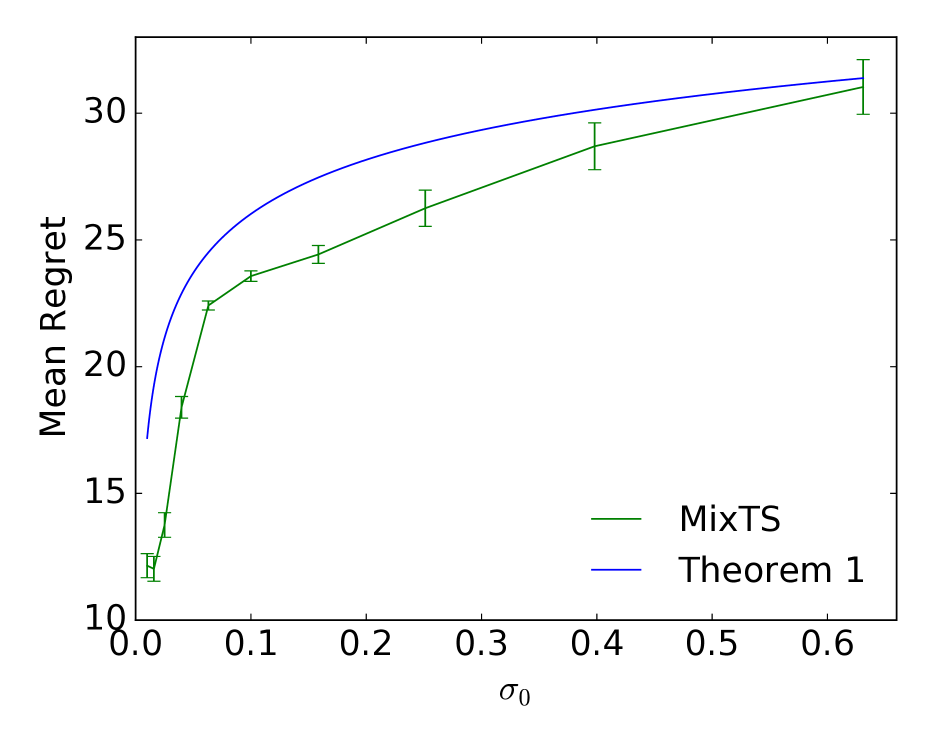
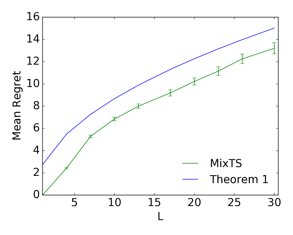
We begin with a synthetic -dimensional Gaussian linear bandit where . We consider up to latent states. The latent state prior is uniform, for each . The model parameter prior is an isotropic Gaussian . The -th entry of is when , and otherwise. The action set is constant over all rounds and consists of all -dimensional indicator vectors. The reward for action is sampled from a Gaussian with . The horizon is rounds. We run times, with and sampled from the prior at the beginning of each run. We vary two quantities in Theorem 1, the prior width and number of latent states , and assess their effect on regret.
For each and , we use the mean regret over multiple runs, where in each run, model parameters are drawn as , to approximate the Bayes regret. The regret is reported in Figure 1, together with the upper bound in Theorem 1. The upper bound is multiplied by , which changes the scale but preserves the shape. We observe that our bound correctly estimates the shape of the empirical regret as a function of . In a similar experiment, where is fixed and we vary the number of latent states , we again observe that our bound correctly estimates the shape of the empirical regret as a function of . We conclude that Theorem 1 scales correctly with the parameters of our problem class.
6.2 Image Classification
In our second experiment, we consider an image classification problem with a mixture of high-level tasks. We use the CIFAR-100 dataset (Krizhevsky, 2009), which consists of images of size . There are training and test images. Each image belongs to one of classes (image labels).
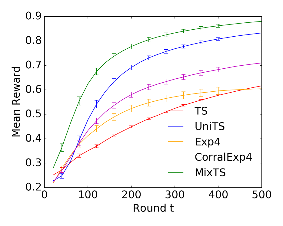
We treat each class as a task, so that images in class have high reward when the task is . At the beginning of each run, a class is sampled as , where for all . In round , the action set consists of randomly chosen images from the CIFAR-100 test set, where one image is guaranteed to be from class . The reward of an image from class is and for all other classes is . The horizon is rounds. For such short horizons, the effect of the prior is more noticeable. We cast this problem as a linear bandit with features from a state-of-the-art EfficientNet-L2 network Xie et al. (2020); Tan and Le (2019); Foret et al. (2021). This is a convolutional neural network pretrained on both ImageNet (Russakovsky et al., 2015) and unlabeled JFT-300M (Sun et al., 2017) with input resolution , and fine-tuned on the CIFAR-100 training set. Each action is a -dimensional feature vector, the embedding after applying the network.
The mixture prior is obtained by clustering similar tasks from the CIFAR-100 training set. This is done as follows. First, we sample random datasets of size from the training set. For each dataset, we randomly choose the class , and assign reward one to images from class and zero otherwise. Second, we fit a linear model to each dataset, where the image features are generated as above. Finally, we fit a GMM with components to the parameter vectors of the trained linear models, generating cluster means and covariances . The model parameter prior for is .
We compare to four baselines: , , (Auer et al., 2002), and . is Thompson sampling with an uninformative Gaussian prior over model parameters. is TS with a unimodal Gaussian prior fit to the same data as the GMM. This baseline shows the importance of using mixtures, as opposing to just using past data. uses the prior means as experts, where the action of expert is . The actions are a weighted vote of the experts, where better experts have higher weights. Finally, uses to track experts, but additionally adapts the parameters of each expert so that in round , the action of expert is , where is defined as in (4). is an instance of a corralling bandit algorithm (Maillard and Munos, 2011; Agarwal et al., 2017; Arora et al., 2021), where a master () switches between base algorithms (linear regressors). We measure the mean reward of each method, averaged over independent runs. Note that all TS algorithms are misspecified in this experiment, because the models are not linear and the reward noise is not Gaussian. We use since the rewards are in . As shown in Figure 1, greatly outperforms and , especially during the cold-start regime, due to using a strong mixture prior fitted to existing data. also outperforms and by explicitly leveraging the latent state posterior to switch between models. Although uses the same model updates, it switches between the models using an adversarial algorithm.
6.3 Synthetic MDP
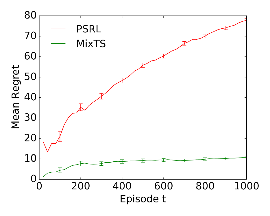
In our final experiment, we consider a synthetic finite-horizon MDP based on the RiverSwim environment (Osband et al., 2013). RiverSwim consists of states arranged in a chain. The agent starts at the state in the middle and at every time step, can choose to swim right or left, . The environment is parameterized by a latent state that denotes the direction of the current, which can be right or left, . At a high level, swimming with the current is always successful, but swimming against the current likely fails. If the current is to the left, the agent receives a small reward for swimming left at the leftmost state, but receives a much larger reward for swimming right at the rightmost state; if the current is to the right, the opposite holds. The optimal policy involves swimming against the current to receive the large reward. The prior mean MDP when the current is to the left is shown in Figure 2. The MDP when the current is to the right is symmetric.
In our experiments, we consider and horizon . The latent state prior is uniform, for as left or right. The MDP prior, conditioned on each latent state, consists of beta and Dirichlet priors for the mean reward and transition probabilities for each state-action pair , such that the mean MDP under the prior matches the values in Figure 2. The number of episodes is episodes, and we run times on independent samples of the MDP from the prior. In Figure 2, we compare the mean regret over the runs of against PSRL (Osband et al., 2013), which is a TS algorithm that uses a uniform prior over rewards and transitions. greatly outperforms PSRL because it identifies the correct latent state, or direction of the current, much more quickly than PSRL learns the reward and transitions from scratch.
7 RELATED WORK
Thompson sampling. Thompson sampling is known for its computational efficiency and strong empirical performance (Agrawal and Goyal, 2012; Chapelle and Li, 2012; Agrawal and Goyal, 2013). Russo and Van Roy (2013) derived first Bayes regret bounds for TS in bandits and RL (Osband et al., 2013). We build on these works by considering a mixture prior. By explicitly modeling a latent state, we can implement TS efficiently, as well as derive improved prior-dependent Bayes regret bounds. Alternatively, information theory has been used to derive Bayes regret bounds (Russo and Van Roy, 2016; Lu and Van Roy, 2019). These proofs rely on the entropy of posterior distributions, which do not have closed forms for mixtures. Recent works applied approximate TS to complex structured problems (Gopalan et al., 2014; Yu et al., 2020). Such algorithms are general, but can only be analyzed in limited settings with strong assumptions. We consider a special prior structure, and derive improved regret bounds for bandits and RL.
A related work on TS with mixture distributions is Urteaga and Wiggins (2018). The setting of this work is completely different because they study a mixture reward distribution. In comparison, we study a mixture of model parameters. To make this distinction clear, consider a linear bandit. Urteaga and Wiggins (2018) would have non-Gaussian rewards sampled from a Gaussian mixture model (GMM). We would have Gaussian rewards with model parameters sampled from a GMM. More recently, Urteaga and Wiggins (2021) proposed a non-parametric GMM over the rewards in the bandit setting. This is another instance of a mixture reward distribution.
Online model selection. Our work is also related to online model selection, as each latent state corresponds to a different hypothesis for the distribution of the environment. Identifying the true latent state is analogous to selecting the best-performing base model. (Auer et al., 2002) is one of the earliest algorithms for solving this problem in adversarial environments. Bayesian policy-reuse (BPR) (Rosman et al., 2016) could be used in stochastic environments but it does not have theoretical guarantees. More recently, in corralling bandits, a master algorithm learns the best-performing base bandit algorithm. Maillard and Munos (2011) proposed a modified version of as the master. Corralling algorithms have also been extended to the stochastic setting (Agarwal et al., 2017; Arora et al., 2021; J. Foster et al., 2019). In all above works, the base algorithm is updated only when selected by the master. In our work, because of the full Bayesian treatment, all mixture components are always updated, which increases statistical efficiency. As shown in Section 6, outperforms multiple online model selection baselines.
Latent bandits. Our setting is also an instance of latent bandits, where bandit instances are parameterized by a finite set of latent states, and each one corresponds to a different hypothesis over reward models (Maillard and Mannor, 2014; Zhou and Brunskill, 2016; Hong et al., 2020). In such structured environments, it is natural to consider a mixture prior that is learned from existing data, each component of the prior being a model distribution. However, most previous works only considered a single fixed model per latent state (Maillard and Mannor, 2014). The closest work is Hong et al. (2020), who proposed a TS algorithm . In a bandit, is an instance of where the conditional models are mixture components and share the same parameter space. This distinction is important, as we explicitly analyze the concentration of the mixture posterior to derive sublinear regret bounds. The regret bounds of Hong et al. (2020) are agnostic to posterior improvements and can be linear. We also apply to reinforcement learning, which in turn generalizes .
8 CONCLUSIONS
We propose Thompson sampling with a mixture prior () for online decision making. The mixture prior is parameterized by a discrete latent state, and yields a general and tractable algorithm that can be broadly analyzed, in both bandit and RL settings. Our regret bounds reflect the structure of the prior, the number of mixture components and their widths. We evaluate on both synthetic and an image classification problems, and demonstrate that it performs well.
This work is a step towards analyzing TS in realistic models with latent variables. Our regret bounds depend on the number and width of the prior mixture components, but not on the latent state prior, which leaves room for improvement. We also only consider a flat discrete latent state. More expressive latent structures are an interesting direction for future work.
References
- Abbasi-yadkori et al. (2011) Y. Abbasi-yadkori, D. Pál, and C. Szepesvári. Improved algorithms for linear stochastic bandits. NeurIPS, 2011.
- Abeille and Lazaric (2017) M. Abeille and A. Lazaric. Linear thompson sampling revisited. In AISTATS, 2017.
- Agarwal et al. (2017) A. Agarwal, H. Luo, B. Neyshabur, and R. E. Schapire. Corralling a band of bandit algorithms. In COLT, 2017.
- Agrawal and Goyal (2012) S. Agrawal and N. Goyal. Analysis of Thompson sampling for the multi-armed bandit problem. 2012.
- Agrawal and Goyal (2013) S. Agrawal and N. Goyal. Thompson sampling for contextual bandits with linear payoffs. ICML, 2013.
- Agrawal and Jia (2017) S. Agrawal and R. Jia. Posterior sampling for reinforcement learning: worst-case regret bounds. In NeurIPS, 2017.
- Arora et al. (2021) R. Arora, T. V. Marinov, and M. Mohri. Corralling stochastic bandit algorithms. In AISTATS, 2021.
- Auer et al. (2002) P. Auer, N. Cesa-Bianchi, Y. Freund, and R. E. Schapire. The nonstochastic multiarmed bandit problem. In SIAM Journal of Computing, 2002.
- Ayoub et al. (2020) A. Ayoub, Z. Jia, C. Szepesvári, M. Wang, and L. F. Yang. Model-based reinforcement learning with value-targeted regression. In ICML, 2020.
- Barto and Sutton (2018) A. Barto and R. S. Sutton. Reinforcement Learning: An Introduction. MIT Press, Cambridge, 2018.
- Bellman (1957) R. Bellman. A Markovian decision process. Indiana University Mathematics Journal, 6, 1957.
- Bishop (2006) C. Bishop. Pattern Recognition and Machine Learning. Springer New York, 2006.
- Blei et al. (2003) D. M. Blei, A. Y. Ng, and M. I. Jordan. Latent Dirichlet allocation. JMLR, 2003.
- Burnetas and Katehakis (1997) A. N. Burnetas and M. N. Katehakis. Optimal adaptive policies for Markov decision processes. Mathematics of Operations Research, 22, 1997.
- Chapelle and Li (2012) O. Chapelle and L. Li. An empirical evaluation of Thompson sampling. In Neural Information Processing Systems, pages 2249–2257, 2012.
- Foret et al. (2021) P. Foret, A. Kleiner, H. Mobahi, and B. Neyshabur. Sharpness-aware minimization for efficiently improving generalization. In ICLR, 2021.
- Gopalan et al. (2014) A. Gopalan, S. Mannor, and Y. Mansour. Thompson sampling for complex online problems. In ICML, 2014.
- Hong et al. (2020) J. Hong, B. Kveton, M. Zaheer, Y. Chow, A. Ahmed, and C. Boutilier. Latent bandits revisited. In NeurIPS, 2020.
- J. Foster et al. (2019) D. J. Foster, A. Krishnamurthy, and H. Luo. Model selection for contextual bandits. In NeurIPS, 2019.
- Jordan and Jacobs (1994) M. I. Jordan and R. A. Jacobs. Hierarchical mixtures of experts and the em algorithm. Neural Computation, 1994.
- Krizhevsky (2009) A. Krizhevsky. Learning multiple layers of features from tiny images. 2009.
- Lai (1987) T. L. Lai. Adaptive treatment allocation and the multi-armed bandit problem. The Annals of Statistics, 15(3):1091 – 1114, 1987.
- Lattimore and Szepesvári (2019) T. Lattimore and C. Szepesvári. Bandit Algorithms. Cambridge University Press, 2019. doi: 10.1017/9781108571401.
- Lu and Van Roy (2019) X. Lu and B. Van Roy. Information-theoretic confidence bounds for reinforcement learning. In NeurIPS, 2019.
- Macqueen (1967) J. Macqueen. Some methods for classification and analysis of multivariate observations. In Berkeley Symposium on Mathematical Statistics and Probability, 1967.
- Maillard and Mannor (2014) O.-A. Maillard and S. Mannor. Latent bandits. In ICML, 2014.
- Maillard and Munos (2011) O.-A. Maillard and R. Munos. Adaptive bandits: Towards the best history-dependent strategy. In AISTATS, 2011.
- Marchal and Arbel (2017) O. Marchal and J. Arbel. On the sub-Gaussianity of the Beta and Dirichlet distributions. CoRR, abs/1705.00048, 2017.
- Osband et al. (2013) I. Osband, B. Van Roy, and D. Russo. (More) efficient reinforcement learning via posterior sampling. In NeurIPS, 2013.
- Rosman et al. (2016) B. Rosman, M. Hawasly, and S. Ramamoorthy. Bayesian policy reuse. Machine Learning, 2016.
- Russakovsky et al. (2015) O. Russakovsky, J. Deng, H. Su, J. Krause, S. Satheesh, S. Ma, Z. Huang, A. Karpathy, A. Khosla, M. Bernstein, A. C. Berg, and L. Fei-Fei. ImageNet Large Scale Visual Recognition Challenge. International Journal of Computer Vision (IJCV), 115(3):211–252, 2015. doi: 10.1007/s11263-015-0816-y.
- Russo and Van Roy (2013) D. Russo and B. Van Roy. Learning to optimize via posterior sampling. CoRR, abs/1301.2609, 2013.
- Russo and Van Roy (2016) D. Russo and B. Van Roy. An information-theoretic analysis of thompson sampling. In Journal of Machine Learning Research, 2016.
- Sun et al. (2017) C. Sun, A. Shrivastava, S. Singh, and A. Gupta. Revisiting unreasonable effectiveness of data in deep learning era. In 2017 IEEE International Conference on Computer Vision (ICCV), pages 843–852, 2017. doi: 10.1109/ICCV.2017.97.
- Tan and Le (2019) M. Tan and Q. Le. EfficientNet: Rethinking model scaling for convolutional neural networks. In ICML, pages 6105–6114, 2019.
- Urteaga and Wiggins (2018) I. Urteaga and C. H. Wiggins. Variational inference for the multi-armed contextual bandit. In AISTATS, 2018.
- Urteaga and Wiggins (2021) I. Urteaga and C. H. Wiggins. Nonparametric Gaussian mixture models for the multi-armed contextual bandit. CoRR, abs/1808.02932, 2021.
- Wang (2001) J. Wang. Generating daily changes in market variables using a multivariate mixture of normal distributions. In Proceedings of the 33rd Winter Conference on Simulation, 2001.
- Xie et al. (2020) Q. Xie, M.-T. Luong, E. Hovy, and Q. V. Le. Self-training with noisy student improves imagenet classification. In Proceedings of the IEEE/CVF Conference on Computer Vision and Pattern Recognition (CVPR), June 2020.
- Yu et al. (2020) T. Yu, B. Kveton, Z. Wen, R. Zhang, and O. J. Mengshoel. Graphical models meet bandits: A variational Thompson sampling approach. In ICML, 2020.
- Zhou and Brunskill (2016) L. Zhou and E. Brunskill. Latent contextual bandits and their application to personalized recommendations for new users. In IJCAI, 2016.
Appendix A Linear Bandit Proofs
A.1 Useful Lemmas
Lemma 1.
Let be a random vector sampled from the multivariate Gaussian . For any , define event . Then,
Proof.
Using that , we can conclude that has independent Gaussian entries. We have
where we use that implies , and consider each entry of separately. ∎
Lemma 2.
For round and latent state , let be defined as in (4). If for all , then for any such that , then
Proof.
The proof is similar to that done for Lemma 11 of Abbasi-yadkori et al. (2011). Instead, we consider the norm with respect to posterior covariance rather than empirical covariance .
We have,
where we use the matrix determinant lemma, which says for matrix and vector . Note that
so if , then . Using that for , we get,
This yields
as desired. ∎
A.2 Proof of Theorem 1
In the outline, we were able to trivially bound the regret of each round by ; this is no longer the case since is a sample from a Gaussian. To handle this, we introduce event
which occurs when is not far from its prior mean. We can bound the regret by,
When occurs, the regret for a round can be arbitrarily large; to handle this, we factor in that is unlikely. Fix round . We bound the regret in round as
where we use the Cauchy-Schwartz inequality, and for any action and latent state . Since , we have and
where we apply Lemma 1 with . Hence, we can bound the Bayes regret as
When occurs, we have is an upper-bound on regret for a round. We use .
From here, we can follow the analysis outline in Section 4.1 using defined as
Using Equation 1, we can decompose the Bayes regret in a linear bandit as
| (9) |
We bound each term individually.
Step 1.
Let us first consider the first term of (9). Fix round . Let us define event
which occurs when is not far from the mean of conditional posterior . Note that from earlier. We can bound
where we use that when occurs, we have
Now, when occurs, we have
where we again use Cauchy-Schwartz and for any action and latent state .
Step 2.
We define as a high-probability set around latent states using the following construction:
where and
is the \sayover-estimation of the predicted rewards under a latent state and the realized reward. We show that holds with high probability for any round via the following lemma.
Lemma 3.
For any round , .
Proof.
We know that occurs if is not too large. On a high-level, our goal is to upper-bound by a martingale with respect to history, then bound the probability that is too large using Azuma’s inequality for concentration of martingales.
For , we know that . Let us define
as the event that is not too far from its posterior mean. Let be the event that this holds for all rounds up to round and be the complement. We know that
which implies that
| (10) |
We will bound each probability individually. For the first probability of (10), we simply have
where we use that for and round , we have is the sum of independent Gaussians. Then, we take an expectation over histories, and use a union bound over latent states and rounds.
Now, consider the second probability in (10). Fix , and let be the rounds where is sampled up to round . Also, let . Observe that , so that is a martingale difference sequence with respect to histories . We have
where we use Cauchy-Schwartz in the inequality. This implies that
For any round , and latent state , we have that is a random quantity. First, we fix where and yield the following due to Azuma’s inequality,
Finally, by the union bound, we have
Combining the two bounds completes the proof. ∎
Step 3.
Now, we consider the second term of (9). We have,
where we use that conditioned on , are i.i.d. to get From Lemma 3, the first term is . From the outline in Section 4.1, we have
The last term can be bounded as
where for latent state , and as the last round that a latent state is acted upon, we use that there is an upper-bound on by definition of . We trivially bound the regret by for the last round is acted upon.
Hence, we can bound the second term of (9) by
What remains is bounding the sum of confidence widths. We have
where we first use that for latent states differ among one another only through their prior, and then use Lemma 2 to bound the sum of norms. We use the determinant-trace inequality to bound,
where we use that
Combining the bounds across all steps yields
∎
Appendix B Tabular MDP Proofs
B.1 Useful Lemmas
Lemma 4 (Theorem 1 and 3 of Marchal and Arbel (2017)).
Let for . Then is -sub-Gaussian with . Similarly, let for . Then is -sub-Gaussian with .
Lemma 5 (Value difference lemma).
For any MDPs , , and policy ,
Lemma 6.
Proof.
The proof is similar to that done in Osband et al. (2013). However, we use prior-dependent definitions for the confidence width . First, we define as the number of times were sampled up to episode . We can decompose the sum as
where we trivially bound the regret in a step of an episode by . Therefore, the first term is bounded as .
For the second term, let us additionally define as the number of times were sampled up to step of episode . Now, if , then we know that . We consider of individually. We have
where for the last inequality, we use that for any ,
Similarly, we have
Combining the two bounds yields
∎
B.2 General Analysis Outline
Step 1.
Bound the Bayes regret due to the first term of (6). For episode , we introduce event
to denote when the sampled mean rewards and transitions are not far from their posterior means for all state-action pairs. Using Lemma 5, we know that
where . Here, we take an expectation over MDPs to apply Lemma 5, then condition on occurring. The second term can be bounded as a sum of confidence widths, and the remaining term can be bounded by using that conditioned on , is unlikely.
Step 2.
For each episode , construct such that with high probability. To do so, we define as the number of times was acted upon and
as the total over-estimation of observed returns by assuming that is the true latent state, where is a scaling factor. Here, we use the shorthand . Then we define as containing all latent states where . Note that we scale by an additional over the outline for bandits in Section 4.1 to account for taking the summation over a trajectory. We show that for any episode , . This means that with high probability, the true latent state lies in .
Step 4.
We can decompose the second term of (6) as
where we use that conditioned on , latent states are identically distributed. From Step 1 and 2, we know that the second term is bounded as . Finally, the remaining term can be bounded as
where we use that . The second can be bounded as the sum of confidence widths, which concentrate over time. The remaining term can be bounded by the sum of gaps , which we know is bounded by after trivially bounding the regret the last time each latent state is acted upon by .
B.3 Proof of Theorem 2
Recall from the proof sketch in Section 5.1 that is the expected value of a policy under state , marginalized over MDPs sampled from its conditional posterior for episode . We want to bound each term of the regret decomposition in (6) separately.
Step 1.
For episode , let
denote the event that the sampled mean rewards and transitions are not far from their posterior means for all state-action pairs. From the sketch in Section B.2, we rewrite the first term of (6) as
For each episode , we can use that to yield
where the second inequality uses that and the third uses the sub-Gaussian parameter given in Lemma 4. Similarly, since , we have
Now, using Lemma 4 for Dirichlet distributions, we have
So, we can bound the first term of (6) by
Step 2.
For each episode , we define as follows:
where is the number of times was sampled from the posterior and is defined as
We show that holds with high probability for any episode via the following lemma.
Lemma 7.
For any episode , .
Proof.
Fix . We know that occurs as long as is not too large. Let us define as the episodes where is sampled until episode . We want to upper-bound by a martingale with respect to history, then bound the probability that is too large using Azuma’s inequality for concentration of martingales.
Let us define
as the event that the mean reward and transition probabilities for episode of episode are not far from their posterior means. Let be the event that this holds for all episodes and steps and be the complement. We know that
where we use that we have and follow a Beta and Dirichlet distribution, respectively, which are sub-Gaussian from Lemma 4.
For episode , let . Observe that , so that is a martingale difference sequence with respect to histories . Also note that since the sum of Bernoulli random variables and is therefore -sub-Gaussian with . We know that conditioned on ,
where we use Lemma 5 to bound . This implies that conditioned on , we have
For any episode , we have that is a random quantity. First, we fix where and yield the following due to Azuma’s inequality,
Finally, by the union bound, we have
This completes the proof. ∎
Step 4.
Following the sketch of Section B.2, we can rewrite the second term of (6) as
From Step 1 and 2, the second term is bounded as . Finally, the remaining term can be bounded as
where we use that up until the last episode a latent state is sampled from the posterior, there is an upper-bound on its overestimation .
Let represent at least how concentrated the reward and transition priors are for latent state . Let be the minimum over latent states. What remains the bounding the sum of confidence widths, which is done in Lemma 6. Combining the regret due to both terms gives,
∎