1 Introduction

A well-known fact in finite group theory equates the sum of squares of dimensions of irreducible representations (irreps) to the order of the group $G$. Letting $R$ label the irreps and denoting the dimensions by $d_{R}$, we have

$$\displaystyle|G|=\sum_{R}d_{R}^{2}$$ (1.1)

where $|G|$ is the order of the group. Another well-known fact equates the number of irreps to the number of conjugacy classes. These are two properties of the set of irreps which can be constructed using the combinatorics of group elements and their group multiplication. It is natural to ask whether this combinatoric constructibility of properties of $d_{R}$ goes further to allow reconstruction of all the individual $d_{R}$. A remarkable fact about finite groups is that ${|G|\over d_{R}}$ is an integer for every $R$. The proof, which relies on properties of algebraic integers, involves the intersection of number theory and group theory (see for example [1] for the proof). In this paper, we will describe an algorithm for the construction of the integers $|G|^{2}/d_{R}^{2}$, and hence of $d_{R}$, from the combinatoric data of group multiplications. The multiplications are shaped according to the fundamental groups of two dimensional surfaces.

Many interesting results in representation theory have combinatoric constructions. For example the enumeration of representations of the symmetric group can be done by enumerating Young diagrams. The computation of dimensions $d_{R}$ for irreps of symmetric groups can be done by counting standard Young tableaux. The Littlewood-Richardson coefficient can be computed by a combinatoric rule for composing Young diagrams. These results are described in standard textbooks on representation theory, e.g. [2]. Further results along these lines are given in [3]. A number of open problems in representation theory revolve around finding combinatoric interpretations for representation theoretic quantities [4]. Such interpretations have implications for computational complexity theory [5, 6, 7, 8, 9]. In a recent paper [10], it was shown that stringy combinatoric structures, notably bipartite ribbon graphs, can be used to provide a lattice interpretation for Kronecker coefficients. The stringy nature of bipartite graphs reveals itself in a number of ways [11, 12, 13, 14, 15].

Here we turn to the question of whether string theory can provide an avenue for the constructibility of $d_{R}$ and ${|G|\over d_{R}}$. A number of developments in topological field theory and topological string theory, provide valuable hints in this direction. Our constructions will be based on the topological field theory of flat $G$-bundles on two dimensional surfaces, which has concrete realizations as lattice constructions [16, 17, 18, 19]. We will refer to this topological field theory based on $G$ as $G$-TQFT2. Recent work in connection with wormhole physics and baby universes [20, 21] has introduced sums over surfaces weighted by a string coupling $g_{st}$, where each surface supports a $G$-TQFT2, thus defining topological string theories based on $G$-TQFT2. We will refer to these string theories as combinatoric topological string theories or $G$-CTST. We will give a construction of $\left({|G|/d_{R}}\right)^{2}$ which involves collecting $G$-TQFT2 data from surfaces surfaces of different genera, so the construction may be naturally interpreted in terms of $G$-CTST. $G$-TQFT2 have been used as an alternative approach to proving the integrality of the ratios $|G|/d_{R}$ in the mathematics literature in [22].

While the paper starts with these motivations based on representation theoretic construction algorithms related to $G$-TQFT2/$G$-CTST, we then turn to physical questions related to these theories and it turns out that these ratios continue to play a key role. We describe transition probabilities constructed from $G$-TQFT2, from disjoint unions of circles to disjoint unions of circles, using the topological lattice formulation as a model for a two-dimensional path integral. As usual the probabilities are squares of amplitudes computed from the path integral. The algebraic structure of $G$-TQFT2 ensures that the amplitudes themselves are sums over sectors labelled by irreducible representations of $G$. The weights include the Plancherel distribution over irreps of finite groups [23] and various generalizations (depending on the choice of genus of the interpolating surfaces), which find a geometrical interpretation as amplitudes in $G$-TQFT2. The sums over sectors labelled by irreps are interpreted following [20] as sums over the $\alpha$-states, which were identified by Coleman [24] as part of a mechanism to restore quantum coherence in the context of wormhole physics. Using some of the algebraic structures of $G$-TQFT2 developed in the context of open-closed topological string theory [25], we find that regarding the centre of the group algebra of $G$, denoted ${\cal Z}(\mathbb{C}(G))\equiv{\cal H}$, as a quantum mechanical Hilbert space gives a useful way to think about the one-dimensional topological quantum mechanics underlying $G$-TQFT2 and its two-dimensional geometrical structures. The integer ratios ${|G|\over d_{R}}$ play a central role in this discussion. Denoting as $P_{R}$ the projector basis elements of ${\cal Z}(\mathbb{C}(G))$, there is a handle-creation operator

$$\displaystyle\Pi=\sum_{R}\left({|G|\over d_{R}}\right)^{2}P_{R}$$ (1.2)

which can also be expressed in terms of the structure constants of ${\cal Z}(\mathbb{C}(G))$ [26, 19].

Considering the sums of $G$-TQFT2 amplitudes over all genera which define $G$-CTST as in [20, 21] we investigate the stringy property of $S$-duality. We then study the finiteness properties of $G$-TQFT2/$G$-CTST and their physical implications. This leads to the definition of an inner product for a polynomial algebra of surfaces, where the null states capture the finiteness relations. This draws on the study of giant gravitons [27, 28, 29] in the context of AdS5/CFT4, notably features such as the departure from large $N$ factorization and their connection to finiteness and the holographic map for large operators [31, 30]. As we explain, $G$-TQFT2 amplitudes play a mathematical role analogous to trace-observables of CFT4. This leads to the consideration of a 2D/3D holographic duality involving $G$-TQFT2. The discussion gives a new perspective on the factorization puzzle associated with 3D wormholes in 2D/3D holography [32].

The paper is organized as follows. In Section 2 we explain how the integer ratios $({|G|\over d_{R}})^{2}$ are constructed from amplitudes of $G$-TQFT2. In section 3 we generalize the discussion to show how to construct the normalized characters of finite groups from boundary amplitudes of $G$-TQFT2. We explain the relation of this construction to existing algorithms for characters. The normalized characters are defined as ${\chi^{R}(g)|{\cal C}|\over d_{R}}$, where $\chi^{R}(g)$ is the character of a group element $g$ in the irrep $R$, $d_{R}$ is the dimension of the irrep, and $|{\cal C}|$ is the number of elements in the conjugacy class ${\cal C}$ containing $g$. In Section 4, we describe probability distributions associated with the interpretation of $G$-TQFT2 in terms of a 2D path integral, and the structure of the amplitudes as sums over irreps. In Section 5 we describe an $S$-duality transformation on closed string amplitudes of $G$-CTST. While the expansion of $G$-CTST at positive powers of the string coupling $g_{st}$ is given in terms of positive powers sums of ${|G|/d_{R}}$, the $S$-dual expansion is in terms of positive power sums of $d_{R}$. We give a geometrical interpretation of these positive power sums in terms of $G$-TQFT2 amplitudes for entangled disconnected surfaces, where the entanglement is defined using projectors $P_{R}$ for the irreps living in the centre ${\cal Z}(\mathbb{C}(G))$ of the group algebra of $G$. In this section we also describe the singularity structure of stringy partition functions of $G$-CTST amplitudes as a function of the string coupling, exhibiting an interesting link between poles and residues of the partition functions and representation theoretic data. Section 6 is a detailed discussion of the implications of the finiteness of $G$ for relations between string amplitudes at different genera. This discussion leads to the introduction of a coupling between TQFT2 for $G$ and TQFT2 for symmetric groups, which we refer to as $\mathbb{C}(G)\times(\mathbb{C}(S))_{\infty}$-TQFT2. Powers of the handle-creation operator $\Pi$ play an important role in this coupling. Section 7 discusses the possibility of a 3D holographic interpretation for $\mathbb{C}(G)\times(\mathbb{C}(S))_{\infty}$-TQFT2 and in that scenario discusses the factorization puzzle associated with wormholes in 2D/3D holography [32].

2 Constructing integer ratios $|G|/d_{R}$ from group products associated with surfaces

In general, group representation theory of a finite group $G$ over the complex numbers $\mathbb{C}$ is not a purely combinatoric subject. It can involve the solution of eigenvalue equations with roots that may not be integer. Many interesting aspects of irreducible representations nevertheless have integrality properties. As we mentioned in the introduction, a striking property is that the dimension of every irrep is a divisor of the order of the group. The group multiplication table is a discrete and finite object. It is natural to ask if there is a simple way to go from the group multiplication table to the integer ratios ${|G|\over d_{R}}$ for any group $G$ while working purely with integers. We show in this section that this is indeed possible and that it involves group multiplications chosen to be of forms determined by two dimensional surfaces, and that the ratios are reconstructed by collecting the amplitudes of $G$-CTST over different genera and performing integer operations on this data.

Take a group $G$. Let $R$ be a label for its irreps, $d_{R}$ the dimension of the irrep. We have the following well-known properties:

$$\displaystyle\hbox{ Number of irreps}=\sum_{R}d_{R}^{0}=\hbox{ Number of conjugacy classes, }$$ (2.1)

while the sum of squares of the dimensions is

$$\displaystyle\sum_{R}d_{R}^{2}=|G|$$ (2.2)

In $G$-TQFT2, defined in terms of a sum of equivalence classes of $G$-bundles, weighted with inverse automorphism, the following equality is known [16, 18, 19]

$$\sum_{R}\left({|G|\over d_{R}}\right)^{2h-2}$$ (2.3)

$$=\hbox{ Number of flat G-bundles on surface of genus $G$ counted with inverse automorphism }$$ (2.4)

$$={1\over|G|}\sum_{g_{1},g_{2},\cdots,g_{2h-1},g_{2h}\in G}\delta([g_{1},g_{2}][g_{3},g_{4}]\cdots[g_{2h-1},g_{2h}])$$ (2.5)

where $[g_{1},g_{2}]=g_{1}g_{2}g_{1}^{-1}g_{2}^{-1}$. This equation has also been studied in the mathematical literature on finite groups and the geometry of surfaces[33, 34].

This follows using Schur’s orthogonality relations for matrix elements in irreducible representations. For any finite group $G$, we have

$$\displaystyle\sum_{g_{1},g_{2}\in G}\sum_{b,c,d=1}^{d_{R}}D^{R}_{ab}(g_{1})D^{R}_{bc}(g_{2})D^{R}_{cd}(g_{1}^{-1})D^{R}_{de}(g_{2}^{-1})=\left({|G|\over d_{R}}\right)^{2}\delta_{ae}$$ (2.6)

Consequently

$$\displaystyle\sum_{g_{1},g_{2},\cdots,g_{2h}\in G}\chi_{R}([g_{1},g_{2}]\cdots[g_{2h-1},g_{2h}])=\left({|G|\over d_{R}}\right)^{2h}d_{R}$$ (2.7)

and hence

$$\displaystyle\sum_{g_{1},g_{2},\cdots,g_{2h}\in G}\delta([g_{1},g_{2}]\cdots[g_{2h-1},g_{2h}]) = {1\over|G|}\sum_{R}\sum_{g_{1},g_{2},\cdots,g_{2h}}d_{R}\chi_{R}([g_{1},g_{2}]\cdots[g_{2h-1},g_{2h}])$$ (2.8)

$$= |G|\sum_{R}\left({|G|\over d_{R}}\right)^{2h-2}$$ (2.9)

$Z_{h}$, the genus $h$ partition function, is then given by

$$Z_{h}={1\over|G|}\sum_{g_{1},g_{2},\cdots,g_{2h-1},g_{2h}\in G}\delta([g_{1},g_{2}][g_{3},g_{4}]\cdots[g_{2h-1},g_{2h}])$$ (2.10)

$$=\sum_{R}\left({|G|\over d_{R}}\right)^{2h-2}$$ (2.11)

This can also be written as

$$\displaystyle Z_{h}=\sum_{P}{1\over|{\rm Aut}(P)|}$$ (2.12)

where $P$ is a flat $G$-bundle which can be identified with an equivalence class of tuples $(g_{1},g_{2},g_{3},g_{4},\cdots,g_{2h-1},g_{2h})$ obeying the condition

$$\displaystyle g_{1}g_{2}g_{1}^{-1}g_{2}^{-1}\cdots g_{2h-1}g_{2h}g_{2h-1}^{-1}g_{2h}^{-1}=id.$$ (2.13)

using the equivalence relation

$$\displaystyle(g_{1},g_{2},\cdots,g_{2h-1},g_{2h})\sim(gg_{1}g^{-1},gg_{2}g^{-1},\cdots,gg_{2h-1}g^{-1},gg_{2h}g^{-1})~{}~{}\hbox{for all }~{}~{}g\in G$$ (2.14)

${\rm Aut}(P)$ is the subgroup which leaves the tuple fixed and is an automorphism of the flat $G$-bundle $P$, $|{\rm Aut}(P)|$ is the order of the group. For any group $G$, the ratio $|G|/d_{R}$ is known to be an integer. A proof based on properties of algebraic integers is given in [35]. This means that while each equivalence class of G-bundles contributes, in general, a rational number to the sum (2.12) the whole sum is an integer. This integrality is not obvious from a topological point of view. This is discussed in [36].

2.1 Combinatoric construction of ${|G|^{2}\over d_{R}^{2}}$

Many interesting integral quantities in representation theory have combinatoric constructions. Examples include the dimensions of symmetric group irreps and the Littlewood-Richardson coefficients. For a general discussion of such problems see [4, 3], For Kronecker coefficients of symmetric groups, a lattice construction based on ribbon graphs and integer matrices arising from permutation group multiplications was recently given [10]. Here we show that the partition functions of $G$-TQFT2 on genus $h$ surfaces also allow us to construct the integers ${|G|^{2}\over d_{R}^{2}}\equiv a_{R}^{2}$ by using

• Group multiplications of shape defined by the fundamental groups of surfaces.

• Searching among divisors of integers.

From (LABEL:Zhirrepflat), the genus one partition function, $Z_{1}$, is the number of conjugacy classes, which we will denote as $K$. The number of power sums we need to construct the set of all ${|G|\over d_{R}}$ is $K$. This means we need $Z_{2},Z_{3},\cdots,Z_{K+1}$. Using Newton’s identities, we get a polynomial of degree $Z_{1}=K$.

It is convenient to define a matrix $X$

$$\displaystyle X={\rm Diag}(a_{1}^{2},a_{2}^{2},\cdots,a_{K}^{2})$$ (2.15)

Using (LABEL:Zhirrepflat) we have

$$\sum_{R}a_{R}^{2}=Z_{2}={\rm tr}X$$ (2.16)

$$\sum_{R}a_{R}^{4}=Z_{3}={\rm tr}X^{2}$$ (2.17)

$$\vdots$$ (2.18)

$$\sum_{R}a_{R}^{2K}=Z_{K+1}={\rm tr}X^{K}$$ (2.19)

We use Newton’s identities to convert these to elementary symmetric functions. In language familiar from the AdS/CFT treatment of branes, consider

$$F(X,x)=\det(x-X)=(x-a_{1}^{2})(x-a_{2}^{2})\cdots(x-a_{K}^{2})$$ (2.20)

$$=x^{K}-({\rm tr}X)x^{K-1}+{1\over 2}(({\rm tr}X)^{2}-{\rm tr}X^{2})x^{n-2}+\cdots+(-1)^{K}(\det X)$$ (2.21)

$$=x^{K}-e_{1}(X)x^{K-1}+e_{2}(X)x^{K-2}+\cdots+(-1)^{K}e_{K}(X)$$ (2.22)

The elementary symmetric functions are

$$e_{0}(X)=1$$ (2.23)

$$e_{1}(X)=\sum_{i}X_{i}$$ (2.24)

$$e_{2}(X)=\sum_{1\leq i<j\leq K}X_{i}X_{j}$$ (2.25)

$$e_{l}(X)=\sum_{1\leq i_{1}<i_{2}<\cdots<i_{l}\leq K}X_{i_{1}}X_{i_{2}}\cdots X_{i_{l}}$$ (2.26)

It is also useful to define $E_{l}(X)=(-1)^{l}e_{l}(X)$ which leads to

$$\displaystyle F(X,x) =x^{n}+E_{1}(X)x^{n-1}+E_{2}(X)x^{n-2}+\cdots+E_{K-1}(X)x+E_{K}(X)$$ (2.28)

$$=\sum_{l=0}^{K}x^{K-l}E_{l}(X)$$

From (LABEL:tft2dat) the coefficients of the powers of $x$ are given in terms of $G$-TQFT2 partition functions. From (LABEL:defFXx) $a_{R}^{2}$ are the zeroes of $F(X,x)$, which is viewed as a polynomial in $x$ with coefficients constructed from $G$-TQFT2 partition functions as above. So to construct the $a_{R}$ from group theoretic combinatoric data, we need to solve the polynomial equation

$$\displaystyle F(X,x)=0$$ (2.29)

The elementary symmetric functions can be expressed in terms of traces of $X$ as

$$e_{k}(X)=\sum_{p\vdash k}{(-1)^{k-\sum_{i}p_{i}}\over\prod_{i}i^{p_{i}}p_{i}!}\prod_{i}({\rm tr}X^{i})^{p_{i}}$$ (2.30)

$$=\sum_{p\vdash k}{(-1)^{k-\sum_{i}p_{i}}\over\prod_{i}i^{p_{i}}p_{i}!}\prod_{i}(Z_{i+1})^{p_{i}}$$ (2.31)

Here $p$ is a partition of $k$, with $p_{i}$ parts of length $i$, so that $\sum_{i}ip_{i}=k$.

$$\displaystyle\det X =\sum_{p\vdash K}{(-1)^{K-\sum_{i}p_{i}}\over\prod_{i}i^{p_{i}}p_{i}!}\prod_{i}({\rm tr}X^{i})^{p_{i}}$$ (2.33)

$$=\sum_{p\vdash K}{(-1)^{K-\sum_{i}p_{i}}\over\prod_{i}i^{p_{i}}p_{i}!}\prod_{i}(Z_{i+1})^{p_{i}}$$

If we did not know that the $a_{1},a_{2},\cdots,a_{K}$ are integers, we would have to solve complicated polynomial factoring algorithms to find them. However, there are simpler algorithms using this integrality (discussed e.g. at [37]).

The numbers $(a_{1}^{2},a_{2}^{2},\cdots,a_{K}^{2})$ are divisors of $\det X$ since $F(X,x=0)=(-1)^{K}\det X$. Let

$$\displaystyle{\rm{Div}}_{0}=\hbox{ Set of divisors of }(-1)^{K}F(X,x=0)$$ (2.34)

Each of the $a_{R}^{2}$ is a divisor of $(-1)^{K}F(X,x=0)$, i.e. an element of ${\rm{Div}}_{0}$. Next note that $(-1)^{K}F(X,x=1)=\prod_{R}(a_{R}^{2}-1)$. Let $r_{i}$ be the roots of $F(X,x=1)$. The $a_{i}^{2}$ are among the $(r_{i}+1)$.

$$\displaystyle{\rm{Div}}_{1}=\hbox{ Set of divisors of }F(X,x=1)\hbox{ shifted up by}~{}1$$ (2.35)

In general

$$\displaystyle{\rm{Div}}_{l}=\hbox{ Set of divisors of }F(X,x=l)\hbox{ shifted up by}~{}l$$ (2.36)

Each element in the list $\{a_{1}^{2},a_{2}^{2},\cdots,a_{K}^{2}\}$ is in the intersection

$$\displaystyle{\rm{Div}}_{0}\cap{\rm{Div}}_{1}\cap{\rm{Div}}_{2}\cdots\cap{\rm{Div}}_{K-1}$$ (2.37)

and the list satisfies

$$\displaystyle\prod_{R}(a_{R}^{2}-l)=(-1)^{K-l}F(X,l)$$ (2.38)

for all $l\in\{0,1,\cdots,K-1\}$.

Claim We show that if we take $K$ of these Divisor sets, and impose the above conditions (2.38), we will uniquely determine the list of $a_{R}^{2}$.

Proof.

$$F(X,x)=\sum_{k=0}^{K}x^{K-k}E_{k}(X)$$

Note that

$$F(X,1)=1+E_{1}(X)+E_{2}(X)+\cdots+E_{K-1}(X)+E_{K}(X)$$ (2.40)

$$F(X,2)=2^{K}+2^{K-1}E_{1}(X)+2^{K-2}E_{2}(X)+\cdots+2E_{K-1}(X)+E_{K}(X)$$ (2.41)

$$F(X,3)=3^{K}+3^{K-1}E_{1}(X)+3^{K-2}E_{2}(X)+\cdots+3E_{K-1}(X)+E_{K}(X)$$ (2.42)

$$~{}~{}~{}~{}~{}~{}~{}~{}~{}\vdots$$ (2.43)

$$F(X,K-1)=(K-1)^{K}+(K-1)^{K-1}E_{1}(X)+\cdots+(K-1)E_{K-1}(X)+E_{K}(X)$$ (2.44)

Rewrite this as

$$F(X,1)-F(X,0)-1=E_{1}(X)+E_{2}(X)+\cdots+E_{K-1}(X)$$ (2.46)

$$F(X,2)-F(X,0)-2^{K}=2^{K-1}E_{1}(X)+2^{K-2}E_{2}(X)+\cdots+2E_{K-1}(X)$$ (2.47)

$$F(X,3)-F(X,0)-3^{K}=3^{K-1}E_{1}(X)+3^{K-2}E_{2}(X)+\cdots+3E_{K-1}(X)$$ (2.48)

$$~{}~{}~{}~{}~{}~{}~{}~{}~{}\vdots$$ (2.49)

$$F(X,K-1)-F(X,0)-(K-1)^{K}=(K-1)^{K-1}E_{1}(X)+\cdots+(K-1)E_{K-1}(X)$$ (2.50)

Note that

$$\displaystyle\begin{pmatrix}F(X,1)-F(X,0)-1\cr F(X,2)-F(X,0)-2^{K}\cr\vdots\cr F(X,K-1)-F(X,0)-(K-1)^{K}\end{pmatrix}=\begin{pmatrix}1&1&\cdots&1\cr 2^{K-1}&2^{K-2}&\cdots&2\cr\vdots\cr(K-1)^{K-1}&(K-1)^{K-2}&\cdots&(K-1)\end{pmatrix}\begin{pmatrix}E_{1}(X)\cr E_{2}(X)\cr\vdots\cr E_{K-1}(X)\end{pmatrix}$$ (2.52)

This is a linear system of equations giving the $F$’s in terms of the $E$’s. The transformation matrix is a non-singular Van der Monde matrix, which means that once we have chosen the $a$’s to reproduce the correct $F(X,0),F(X,1),\cdots,F(X,K-1)$, the $E_{1},\cdots,E_{K-1}(X)$ are also reproduced.

∎

This completes the construction of the ratios ${|G|\over d_{R}}$ from the combinatoric data of $G$-TQFT2 amplitudes. A further interesting question is whether equation (2.37) alone is sufficient (without using (2.38)) to determine the set of $a_{R}$. At the moment, as described above, one must determine the elements belonging to the intersection and then use (2.38) to check that they are correct. Below, we perform some numerical experiments for $G=S_{n}$ in which we study only the intersection of the sets of divisors to determine the optimal $l$ necessary to identify the correct $a_{R}$. For a given $n$, we construct $F(X,0)$. Then we factorize $F(X,0)$ into its prime factors. For example, for $n=3$, $F(X,0)=11664$, which factorizes into $2^{4}\times 3^{6}$. Then we use these prime factors, together with the corresponding exponents to build all possible divisors of $F(X,0)$. In the example above, $2^{e_{2}}\times 3^{e_{3}}$ with $e_{2}=\{0,1,2,3,4\},e_{3}=\{0,1,\cdots,6\}$ will generate all possible divisors. To find all possible divisors of $F(X,1)$, we subtract 1 from the number we build and check if it is a divisor of $F(X,1)$. We follow a similar process to check if the number we build is a divisor of $F(X,2),F(X,3)$ etc. We keep only the elements that are divisors of the set $\{F(X,0),F(X,1),\cdots,F(X,l)\}$. In this way we construct the intersection (2.37) but for arbitrary $l$. We then check if this generates the correct set of $a_{R}$. The smallest $l$ value for which this occurs is denoted by $l_{opt}$. We performed these calculations for $S_{n}$ for $n=3$ up to $n=10$. The results are shown in Table 1.

$n$	$K$	$l_{opt}$
3	3	6
4	5	6
5	7	7
6	11	9
7	15	7
8	22	36
9	30	36
10	42	25

Table 1: Table showing data for the optimal number of divisor sets to correctly determine the set of $a_{R}$ for $S_{n}$. The table shows results for $n=3$ up to $n=10$.

We note that for $S_{n}$ it is indeed possible to construct the $|G|/d_{R}$ at least for small values of $n$ just by studying the intersection of the divisor sets of the $F(X,l)$. We further note that, for the $n$ values considered, the optimal number of divisor sets $l$ is always less than $2K$.

Finally, we note that the power sums on the LHS of (LABEL:knownEq) have an interpretation in terms of string theory for a target space which is a disjoint union of points [38, 39, 40], which implies that the algorithm for converting the power sums to the integers $({|G|\over d_{R}})^{2}$ we have described has an interpretation as a construction of the string amplitudes for a target space point from a finite set of string amplitudes for the disjoint union .

3 Constructing normalized characters from group words and surfaces

Having shown how closed string amplitudes in $G$-TQFT2/$G$-CTST are used to construct the integer ratios $|G|/d_{R}$ and hence the $d_{R}$, we now consider the construction of characters $\chi^{R}(g)$. It turns out that the quantities appearing most directly from $G$-CTST amplitudes are an appropriately normalized form of the characters. Let ${\cal C}_{p}$ be a conjugacy class of $G$ and let $|{\cal C}_{p}|$ be the number of elements in the conjugacy class. We will denote by $T_{p}$ the sum of group elements, in the group algebra $\mathbb{C}(G)$

$$\displaystyle T_{p}=\sum_{g\in{\cal C}_{p}}g$$ (3.1)

$T_{p}$ is a central element of $\mathbb{C}(G)$, i.e. commutes with all elements in $\mathbb{C}(G)$. The normalized characters for ${\cal C}_{p}$ are, for $g\in{\cal C}_{p}$,

$$\displaystyle{|{\cal C}_{p}|\chi^{R}(g)\over d_{R}}={\chi^{R}(T_{p})\over d_{R}}$$ (3.2)

The set of $T_{p}$ for all conjugacy classes spans the centre ${\cal Z}(\mathbb{C}(G))$. Another basis for ${\cal Z}(\mathbb{C}(G))$ is given by the projectors labelled by irreducible representations $R$

$$\displaystyle P_{R}={d_{R}\over|G|}\sum_{g}\chi^{R}(g)g^{-1}$$ (3.3)

The relation between the two bases is a Fourier transformation and plays an important role in this section. We will start in Section 3.1 by giving the key formulae relating amplitudes of $G$-TQFT2 with boundaries to normalized characters, and then describe how these lead to a combinatoric construction of the characters. Since we restrict the discussion to combinatoric construction involving group multiplications and investigation of integer roots of polynomials, the output is the construction of the set of rational normalized characters (which are also integer as we will see) along with a polynomial with integer coefficients characterizing the non-rational characters which live in finite extensions of the rational numbers. In Section 3.2 we review a standard algorithm used for the construction of characters. In Section 3.3 we explain the link between the standard construction and the discussion of Section 3.1. The link originates from the fact that the higher genus amplitudes used in 3.1 come from gluing 3-holed spheres and makes use of the Fourier transform on ${\cal Z}(\mathbb{C}(G)$.

3.1 Construction of normalized characters from higher genus surfaces with boundary

A standard result in $G$-TQFT2 is that the amplitude for a genus $h$ surface with $r$ distinct boundaries, where the group element at the boundary is constrained to be in a conjugacy class ${\cal C}_{p}$ is

$$\sum_{R}\left({|G|\over d_{R}}\right)^{2h-2}\left({\chi_{R}(T_{p})\over d_{R}}\right)^{r}$$ (3.4)

$$={\rm tr}\left(X^{2h-2}X_{p}^{r}\right)$$ (3.5)

$$={1\over|G|}\sum_{s_{i},t_{i}}\sum_{\sigma_{1}.\cdots,\sigma_{r}\in{\cal C}_{p}}\delta\left((\prod_{i=1}^{h}s_{i}t_{i}s_{i}^{-1}t_{i}^{-1})\sigma_{1}\cdots\sigma_{r}\right)$$ (3.6)

$X$ is a diagonal matrix with diagonal entries equal to ${|G|\over d_{R}}$. We have defined $X_{p}$ to be the diagonal matrix with matrix entries $\left({\chi_{R}(T_{p})\over d_{R}}\right)$. Fixing $h=1$, we get power sums of the normalised character from combinatoric data.

$$\displaystyle{\rm tr}(X_{p}^{r}) = \sum_{R}\left({\chi_{R}(T_{p})\over d_{R}}\right)^{r}$$ (3.7)

$$= {1\over|G|}\sum_{s_{1},t_{1}}\sum_{\sigma_{1}.\cdots,\sigma_{r}\in{\cal C}_{p}}\delta(s_{1}t_{1}s_{1}^{-1}t_{1}^{-1}\sigma_{1}\cdots\sigma_{r})$$ (3.8)

This gives the combinatoric data reproducing ${\rm tr}(X_{p}^{r})$. It is the counting of $G$ bundles on genus one surfaces with $r$ punctures where the monodromy around each puncture has the specified conjugacy class. In this way we can construct the characters of all conjugacy classes, using the same algorithm as in section 2. The problem reduces to solving the polynomial equation

$$\displaystyle F(X_{p},x)=\det(X_{p}-x)=0$$ (3.9)

As in Section 2.1, we can find integer solutions by considering the integer factors of $F(X_{p},x=0),F(X_{p},x=1),\cdots$. By factoring out the integer factors from $F(X_{p},x)$ we are left with a polynomial $P_{{\cal C}_{p}}(x)$ for every conjugacy class of a group $G$. For every group we can define a polynomial $P_{G}(x)$ which is obtained by taking the product over all the conjugacy classes

$$\displaystyle\prod_{p}P_{{\cal C}_{p}}(x)$$ (3.10)

and clearing all multiplicities, i.e. replacing any factor $p(x)^{m}$ for $m>1$ by $p(x)$. This polynomial $P_{G}(x)$ is tabulated for non-Abelian groups with order up to $60$ in Appendix B. We have produced these polynomials from known character tables but they are in principle constructible using group multiplications shaped by surfaces with boundaries using (3.7). Note that for symmetric groups, these polynomials are always one. This is due to the fact that the normalized characters for symmetric groups are all integers, a fact which was useful in the ribbon graph lattice algorithm for Kronecker coefficients given recently in [10].

The normalized characters ${\chi^{R}(T_{p})\over d_{R}}$ are algebraic integers, i.e. roots of a polynomial of the form $x^{n}+a_{1}x^{n-1}+\cdots+a_{n}$, where the leading coefficient $1$ and the other coefficients $a_{i}$ are integers. This is a consequence of the fact that they are eigenvalues of an integer matrix $(C_{p})_{q}^{~{}~{}r}=C_{pq}^{~{}~{}r}$ of structure constants of multiplication $T_{p}T_{q}=C_{pq}^{~{}~{}r}T_{r}$. This implies that the traces ${\rm tr}X_{p}^{r}$, which are power sums of the normalized characters are integers. Note that the RHS of (LABEL:bdyamps) and (3.7) can be expressed as a sum over equivalence classes of tuples of group elements satisfying the delta function condition. Each equivalence class is a flat $G$-bundle and has an automorphism group, consisting of group elements $g$ which fix the tuple, when acting by conjugation. In the sum, these equivalence classes are weighted by the inverse order of the automorphism group, so these are in general rational numbers. Nevertheless, the sums in (LABEL:bdyamps) and (3.7) are integer due to the integrality of ${\rm tr}X_{p}^{r}$. This seems to be an interesting, not a priori obvious, property of $G$-bundles.

It is useful to note that there are known general finite algorithms [41] which produce all the matrix elements of irreducible representations over $\mathbb{C}$. They work by going over to the cyclotomic field $Q_{e}$, where $e$ is the exponent of the group, i.e. the smallest positive integer such that $g^{e}$ is the identity for all the group elements. Our discussion above works for each fixed conjugacy class and produces the integer normalized characters along with a polynomial ${\cal P}_{{\cal C}_{p}}(x)$ which defines an algebraic extension of the rational numbers containing the non-integer normalized characters for that conjugacy class. The non-integer roots will also live in the field $Q_{e_{p}}$ where $e_{p}$ is the smallest positive integer with the property that $g^{e_{p}}$ is the identity for $g$ in the conjugacy class ${\cal C}_{p}$. Typically $e_{p}$ will be much smaller than $e$.

For the symmetric group, the exponent is

$$\displaystyle\prod_{p\leq n}p^{\lfloor\ln(n)/\ln(p)\rfloor}$$ (3.11)

For a short proof, see [42]. However it is known that the normalized characters are rational, for example by the Murnaghan-Nakayama construction [2]. It is a useful fact that if a normalized character is rational, it must be integer. The algorithm for normalized characters we have described will determine all characters that can be expressed without field extensions of the rationals. For a general group, once we the integer characters are determined, we are left with the characters which require an extension of the rationals. It is worth emphasizing that our discussion in this paper is not focused on finding alternative efficient computations of characters to known methods, but to describe combinatoric algorithms that go from group multiplications, of forms determined by two-dimensional surfaces, equivalently from amplitudes of combinatoric topological string theory, to the characters. By this route, we get to all the integer characters for any group and to polynomials ${\cal P}_{{\cal C}_{p}},{\cal P}_{G}$, which have leading term $1$ and integer coefficients, and which characterise the non-integer characters. It would be interesting to consider efficient algorithms and general theoretical characterisation of these polynomials for different choices of $G,{\cal C}_{p}$.

The discussion above has focused on $h=1$. If we use $h=0$, we have instead

$$\sum_{R}{d_{R}^{2}\over|G|^{2}}\left({\chi_{R}(T_{p})\over d_{R}}\right)^{r}={\rm tr}\left(X^{-2}X_{p}^{r}\right)={1\over|G|}\sum_{\sigma_{1}.\cdots,\sigma_{r}\in T_{p}}\delta(\sigma_{1}\cdots\sigma_{r})$$ (3.12)

An interesting problem is to devise algorithms which take these weighted power sums of $\left({\chi_{R}(T_{p})\over d_{R}}\right)$ and produce, as output, the normalized characters. It is intriguing that the $h=1$ data seems to lend itself to known algorithms we have used above, while the $h=0$ case seems less obvious.

3.2 Link to Burnside’s construction

Consider the sum

$$\displaystyle{1\over|G|}\sum_{s,t\in G}\sum_{\sigma\in T_{p}}\,\delta(sts^{-1}t^{-1}\sigma)$$ (3.13)

The geometric interpretation of this sum is that it gives the number of flat $G$-bundles on a torus with a single hole, counted with inverse automorphism. The hole is in state $T_{p}$. Recall that $T_{p}$ is the sum of all elements in conjugacy class ${\cal C}_{p}$ of $G$.We can replace the sum over $s$ by a sum over conjugacy classes ${\cal C}_{q}$. The sum over $s$ above replaces $t$ with $T_{q}$ where $t\in{\cal C}_{q}$. There is also a factor of $|G|/|T_{q}|\equiv|{\rm Sym}({\cal C}_{q})|$ : $\hbox{Sym}({\cal C}_{q})$ is the subgroup of $G$ which commutes with $g\in{\cal C}_{q}$, and $|\hbox{Sym}({\cal C}_{q})|$ is the order of this subgroup. The sum over $t$ then replaces $t^{-1}$ with $T_{q^{\prime}}$ where $t^{-1}\in{\cal C}_{q^{\prime}}$ and the sum over $\sigma$ replaces $\sigma$ with $T_{p}$, so that

$$\displaystyle{1\over|G|}\sum_{s,t\in G}\sum_{\sigma\in T_{p}}\,\delta(sts^{-1}t^{-1}\sigma)=\sum_{q}{1\over|{T}_{q}|}\delta(T_{q}T_{q^{\prime}}T_{p})$$ (3.14)

The right hand side of the last line above has an intuitive geometrical interpretation: it is the partition function of a three holed sphere with the hole in state $T_{q}$ glued to the hole in state $T_{q^{\prime}}$. The third hole is in state $T_{p}$. The delta function is only non-zero when the product of the class functions $T_{q}$, $T_{q^{\prime}}$ and $T_{p}$ multiply to give the identity, with some multiplicity. The identity always sits in a conjugacy class of its own.

As we have discussed in detail above, the sum (3.13) produces a sum over the normalized characters. The last equality above demonstrates that the sums defined by the TQFT are naturally related to the class algebra. This connection has a natural counterpart in constructions of characters starting from the class algebra [43, 44, 45]. Since these known mathematical algorithms are clearly closely related to the construction of characters from TQFT, it is worth reviewing them.

The normalized characters of the conjugacy classes

$$\displaystyle\omega_{Rp}={\chi_{R}(T_{p})\over d_{R}}$$ (3.15)

obey an interesting algebra

$$\displaystyle\omega_{Rp}\omega_{Rq}=\sum_{r}n_{pqr}\omega_{Rr}$$ (3.16)

The fusion coefficients $n_{pqr}$ are integers. The algorithm of Burnside [43] constructs the characters using only algebra, assuming that the fusion coefficients $n_{pqr}$ are known. In practice the calculation of the $n_{pqr}$ can be carried out by multiplication in the group algebra. The algorithm uses the class matrix $N_{p}$ defined by

$$\displaystyle(N_{p})_{qr}=n_{pqr}$$ (3.17)

The class algebra (3.16) implies that $\omega_{Rr}$ is an eigenvector of the class matrix. Setting the identity class to be $r=1$, we see that

$$\displaystyle\omega_{R1}={\chi_{R}(1)\over d_{R}}=1$$ (3.18)

so that if we normalize the eigenvectors of the class matrix so that their first entry is 1, then the $p$th component of the eigenvector is $\omega_{Rp}$. To obtain the characters, we now need the dimensions $d_{R}=\chi_{R}(1)$ of each irrep. By using character orthogonality it is easy to verify that the dimensions are fixed by the sum

$$\displaystyle\sum_{r}{\omega_{Rr}\omega_{Sr}\over|T_{r}|}={\delta_{RS}|G|\over\chi_{R}(1)\chi_{S}(1)}$$ (3.19)

To summarize, Burnside’s algorithm is

• Determine the conjugacy classes of $G$.

• Compute $n_{rst}$ and hence the class matrices $N_{r}$.

• Compute the eigenvalues of each $N_{r}$ normalized so that their first entry is 1. This determines the $\omega_{Rp}$.

• Determine the dimensions $d_{R}$ of the irreps using (3.19).

• Compute $\chi_{R}(T_{p})=\omega_{Rp}d_{R}$.

Subsequent improvements of Burnside’s algorithm were concerned with reducing the computational cost of step 3. See [44, 45] for further details.

3.3 Construction of characters and Fourier transform on the centre of $\mathbb{C}(G)$

The centre of the group algebra ${\cal Z}(\mathbb{C}(G))$ has two natural bases, related by a Fourier transform. The first basis $\{T_{p}\}$ corresponds to conjugacy classes. The second basis set $\{P_{R}\}$ is labelled by irreps. The projectors satisfy

$$\displaystyle P_{R}P_{S}=\delta_{RS}P_{S}$$ (3.20)

A useful property is

$$\displaystyle T_{p}P_{R}={\chi^{R}(T_{p})\over d_{R}}P_{R}$$ (3.21)

The delta function on the group extends to $G$ and gives an inner product on ${\cal Z}(\mathbb{C}(G))$

$$\delta(T_{p}T_{q})=|T_{q}|\delta_{pq^{\prime}}=|T_{q^{\prime}}|\delta_{pq^{\prime}}$$ (3.22)

(3.23)

$$={|G|\over|\hbox{Sym}({\cal C}_{q})|}\delta_{pq^{\prime}}={|G|\over|\hbox{Sym}({\cal C}_{q^{\prime}})|}\delta_{pq^{\prime}}$$ (3.24)

${\cal C}_{q^{\prime}}$ is the conjugacy class which contains the inverses of the group elements in the conjugacy class ${\cal C}_{q}$. The inner product for the projectors is

$$\displaystyle\delta(P_{R}P_{S})=\delta_{RS}{d_{R}^{2}\over|G|}$$ (3.25)

The product in ${\cal Z}(\mathbb{C}(G))$ in the $T_{p}$ basis is

$$\displaystyle T_{p}T_{q}=\sum_{r}C_{pq}^{~{}~{}r}T_{r}=\sum_{r}{\delta(T_{p}T_{q}T_{r^{\prime}})\over|T_{r}|}$$ (3.26)

Consider the identity

$$\displaystyle\sum_{q}{\delta(T_{q}T_{p}^{r}T_{q^{\prime}})\over|T_{q}|}=\sum_{R}{|G|\delta(P_{R}T_{p}^{r}P_{R})\over d_{R}^{2}}$$ (3.27)

which follows from taking the trace of $T_{p}^{r}$ in the two bases. We also have

$$\displaystyle\sum_{q}{T_{q}T_{q^{\prime}}\over|T_{q}|}={1\over|G|}\sum_{g_{1},g_{2}}g_{1}g_{2}g_{1}^{-1}g_{2}^{-1}$$ (3.28)

and

$$\displaystyle\sum_{R}{|G|\delta(P_{R}T_{p}^{r}P_{R})\over d_{R}^{2}}=\sum_{R}{\chi_{R}(T_{p}^{r})\over d_{R}}=\sum_{R}\left({\chi_{R}(T_{p})\over d_{R}}\right)^{r}$$ (3.29)

This leads to

$$\displaystyle{1\over|G|}\sum_{g_{1},g_{2}\in G}\delta(g_{1}g_{2}g_{1}^{-1}g_{2}^{-1}T_{p}^{r})=\sum_{R}\left({\chi_{R}(T_{p})\over d_{R}}\right)^{r}={\rm Tr}(X_{p}^{r})$$ (3.30)

We have thus recovered the identity (3.7) by taking the trace of $T_{p}^{r}$ in the two bases for ${\cal Z}(\mathbb{C}(G)$. The diagram in (3.32) illustrates the geometrical nature of the calculation for $r=2$ :

$$\displaystyle\begin{gathered}\includegraphics[width=32.52017pt]{forcharacter}\end{gathered}\longrightarrow\sum_{q}\delta(T_{q^{\prime}}T_{p}^{2}T_{q}){1\over|T_{q}|}=\sum_{R}\delta(P_{R}T_{p}^{2}P_{R}){1\over\left({d_{R}^{2}\over|G|}\right)}$$ (3.32)

Note that

$$\displaystyle\sum_{q}\delta(T_{q^{\prime}}T_{p}^{2}T_{q}){1\over|T_{q}|} = \sum_{q,r^{\prime}}\delta(T_{q^{\prime}}T_{p}C^{~{}~{}r_{1}}_{pq}T_{r_{1}}){1\over|T_{q}|}$$ (3.33)

$$= \sum_{q,r_{1},r_{2}}C^{~{}~{}r_{1}}_{pq}C_{pr_{1}}^{~{}~{}r_{2}}\delta(T_{q_{1}}T_{r_{2}}){1\over|T_{q}|}$$ (3.34)

$$= \sum_{q,r_{1}}(C_{p})_{q}{}^{r_{1}}(C_{p})_{r_{1}}{}^{r}$$ (3.35)

$$= {\rm Tr}(\tilde{X}_{p}^{2})$$ (3.36)

where $(\tilde{X}_{p})_{q}^{r}=C_{pq}{}^{r}$. From (3.21) we see that the eigenvalues of $\tilde{X}_{p}$ are nothing but the entries of the diagonal matrix $X_{p}$ we defined in Section (3.1).

The connection to Burnside’s algorithm is that the coefficients $C_{pq}^{~{}~{}r}$ are equal to the $n_{pqr}$ appearing in the product of the normalized characters (3.16). The calculation of the eigenvalues of $(N_{p})_{qr}=n_{pqr}=(\tilde{X}_{p})_{q}^{r}$ involves the calculation of

$$\displaystyle\det(\tilde{X}_{p}-\lambda)$$ (3.37)

The coefficients of the powers of $\lambda$ are elementary symmetric polynomials expressible in terms of power sums ${\rm tr}\tilde{X}_{p}^{r}={\rm tr}X_{p}^{r}$. These powers appear in

$$\displaystyle\det(\tilde{X}_{p}-\lambda)=\det(X_{p}-\lambda)$$ (3.38)

Our discussion in Section 3.1 introduced the polynomial $\det(X_{p}-\lambda)$ as a tool to extract the diagonal entries of the matrix $X_{p}$ from the power sums of these entries (a tool which we also used in Section 2 to construct $|G|/d_{R}$), whereas $\det(\tilde{X}_{p}-\lambda)$ arises in Burnside’s construction from the diagonalization of the matrix of structre constants $(N_{p})_{qr}=C_{pq}{}^{r}$.

4 Probability distributions from $G$-TQFT2 and $G$-CTST

The formulation of $G$-TQFT2 as a topological lattice gauge theory with plaquette weight enforcing the flatness condition can be viewed as a discrete path integral in a two-dimensional theory, and realizes the axiomatic formulation of TQFT by Atiyah [46]. This approach to $G$-TQFT2 is a finite group version of [17] which is known to be equivalent to the formulation in [19]. The state space associated with a circle boundary is the centre ${\cal Z}(\mathbb{C}(G))$ of the group algebra $\mathbb{C}(G)$ of $G$. Using the path integral interpretation, it is natural to use the partition function for a $2$-manifold with for $n$ incoming circle boundaries and $m$ outgoing circle boundaries to define probabilities for transitions between ${\cal H}^{\otimes n}$ to ${\cal H}^{\otimes m}$. As we will see the amplitudes are invariant under exchange of the states in the tensor factors, so we have transitions from the symmetrised product $S^{n}({\cal H})$ to $S^{m}({\cal H})$. We will write explicit formulae for the probabilities of such transitions within $G$-TQFT2 and by summing over different genuses with weight $g_{st}^{2h-2}$ we will get analogous transition probabilities for $G$-CTST. The transition probabilities are squares of amplitudes. These amplitudes in turn have an interesting structure, containing a sum over a label $R$ for irreducible representations which contribute according to some positive weights. These positive weights themselves define probability distributions over the irrep labels. These probability distributions include the Plancherel distribution for finite groups [23] and generalizations thereof. Following [20] the sum over $R$ formulae for the amplitudes have an interpretation in terms of a classical ensemble and the irrep labels $R$ provide an example of Coleman’s $\alpha$-eigenstates which were used to explain quantum coherence in the context of wormholes [24, 47]. Building on known structures of $G$-TQFT2 [25], we will review how the sum over irrep sectors arises from the gluing relations of $G$-TQFT2. These are based on the properties of the algebra ${\cal Z}(\mathbb{C}(G))={\cal H}$. The existence of two bases for ${\cal H}$, one labelled by conjugacy classes and one labelled by irreps plays a key role in understanding the sectors. To accommodate the in-out states of the general transition amplitudes between circles, and take advantage to the gluing relations, it is useful to consider quantum mechanics based on the state space

$$\displaystyle\bigoplus_{n=0}^{\infty}S^{n}({\cal H})$$ (4.1)

built from the algebra ${\cal H}$. This may be viewed as a one-dimensional quantum system underlying the sum over $\alpha$-states arising in the amplitudes of $G$-TQFT2.

4.1 Plancherel distribution for $G$ and geometrical generalizations in $G$-TQFT2

The Plancherel distribution makes a natural appearance in the sphere partition function, which is given by the sum

$$\displaystyle Z_{S^{2}}=\sum_{R}\left({d_{R}^{2}\over|G|^{2}}\right)={1\over|G|}$$ (4.2)

The algorithms in Section 3 allow us to use the genus one and higher partition functions to construct the ratios ${|G|\over d_{R}}$. Using these ratios and the formula above, we can add up to recover $Z_{S^{2}}$. In this sense the higher genus partition functions allow us to reconstruct the genus zero partition function.

By multiplying with $|G|$ we have

$$\displaystyle|G|Z_{S^{2}}=\sum_{R}\left({d_{R}^{2}\over|G|}\right)=1$$ (4.3)

The summands are positive numbers which define the Plancherel distribution. We can give an interpretation of each probability in terms of disc partition functions. The disc partition function with boundary condition $g\in G$ is proportional to the delta function on the group

$$\displaystyle|G|Z_{D^{2}}(g)=\delta(g)=\sum_{R}{d_{R}\chi^{R}(g)\over|G|}$$ (4.4)

The disc partition function is defined for group algebra elements $\sum_{g}c_{g}g\in\mathbb{C}(G)$ as

$$\displaystyle Z_{D^{2}}(\sum_{g}c_{g})=\sum_{g}c_{g}Z_{D^{2}}(g)$$ (4.5)

Consider the projector element in $\mathbb{C}(G)$ associated with an irrep $R$

$$\displaystyle P_{R}={d_{R}\over|G|}\sum_{g}\chi_{R}(g)g^{-1}$$ (4.6)

where $\chi_{R}(g)$ is the character of $g\in G$ in irrep $R$.

$$\displaystyle Z_{D^{2}}(P_{R})=\sum_{g}{d_{R}\chi^{R}(g)\over|G|}Z_{D^{2}}(g^{-1})$$ (4.7)

Using (4.4) we find

$$\displaystyle|G|Z_{D^{2}}(P_{R})={d_{R}^{2}\over|G|}$$ (4.8)

This reproduces the probabilities of the Plancherel distribution for a finite group, directly from a disc partition function.

The $G$-TQFT2 perspective on the Plancherel distribution shows that it has a number of generalizations with a geometric interpretation. These generalizations are motivated by considering partition functions for surfaces with $h$ handles and $b$ boundaries. The partition function is

$$\displaystyle Z_{h,b;T_{p_{1}},\cdots,T_{p_{b}}} = \sum_{R}\left({d_{R}\over|G|}\right)^{2-2h-b}\chi^{R}(T_{p_{1}})\cdots\chi^{R}(T_{p_{b}})$$ (4.9)

$$= {1\over|G|}\delta(\Pi^{h-1}T_{p_{1}}\cdots T_{p_{b}})$$ (4.10)

where $\Pi$ is the handle-creation operator

$$\displaystyle\Pi = \sum_{R}\left({|G|\over d_{R}}\right)^{2}P_{R}$$ (4.11)

$$= \sum_{g_{1},g_{2}\in G}g_{1}g_{2}g_{1}^{-1}g_{2}^{-1}=\sum_{p}T_{p}T_{p^{\prime}}~{}|\hbox{Sym}({\cal C}_{p})|$$ (4.12)

This partition function is normalized so that it is consistent with natural geometrical gluing relations as we now explain. Gluing is performed using the inverse cylinder and the boundary in state $T_{p}=\sum_{g\in{\cal C}_{p}}g$ is glued to a boundary in state $T_{p}^{\prime}=\sum_{g\in{\cal C}_{p}}g^{-1}$, and summing the label $p$ over all the conjugacy classes of $G$. We can absorb the factors associated to the inverse of the cylinder in the definition

$$\displaystyle T_{p}^{*}={T_{p^{\prime}}\over|T_{p}|\,|G|}$$ (4.13)

A basic identity that can be used to perform any gluing is

$$\displaystyle\sum_{p}\chi_{R}(AT_{p})\chi_{S}(T_{p}^{*}B)=\sum_{p}{\chi_{R}(AT_{p})\chi_{S}(T_{p^{\prime}}B)\over|T_{p}|\,|G|}=\delta_{RS}\chi_{R}(AB)$$ (4.14)

where $A$ and $B$ to belong to $\mathbb{C}(G)$ and at least one is in the centre ${\cal Z}(\mathbb{C}(G))$. It is also useful to have the gluing equation in terms of projectors :

$$\displaystyle\delta(AB)=\sum_{R}\delta(AP_{R})\delta(P_{R}B){|G|\over d_{R}}$$ (4.15)

where we also require $A$ and $B$ to belong to $\mathbb{C}(G)$ and at least one is in the centre ${\cal Z}(\mathbb{C}(G))$. As an example of some gluing relations, gluing a disc to a $b$ holed sphere gives a sphere with $b-1$ holes

$$\displaystyle\sum_{p}Z_{D^{2}}(T_{p})Z_{h,b;T_{p_{1}},\cdots,T_{p_{b-1}}T_{p}^{*}}=Z_{h,b;T_{p_{1}},\cdots,T_{p_{b-1}}}$$ (4.16)

and gluing two holes increases the number of handles by 1 and decreases the number of boundaries by 2

$$\displaystyle\sum_{p}Z_{h,b;T_{p_{1}},\cdots,T_{p_{b-2}}T_{p}T_{p}^{*}}=Z_{h+1,b-2;T_{p_{1}},\cdots,T_{p_{b-2}}}$$ (4.17)

As mentioned above, the Plancherel distribution admits a number of interesting generalizations.

We can consider a $G$-TFT2 map from $n$ holes to $m$ holes. Associate $T_{p_{1}}\cdots T_{p_{n}}$ to the initial holes and $T_{q_{1}^{\prime}}\cdots T_{q_{m}^{\prime}}$ to the final holes. The relevant partition function, for a surface with $h$ handles, is given by

$$\displaystyle Z_{h,m+n,T_{p_{1}}\cdots T_{p_{n}}T_{q_{1}}^{*}\cdots T_{q_{m}}^{*}} = \sum_{R}\left({d_{R}\over|G|}\right)^{2-2h-m-n}\chi^{R}(T_{p_{1}})\cdots\chi^{R}(T_{p_{n}})\chi^{R}(T_{q_{1}}^{*})\cdots\chi^{R}(T_{q_{m}}^{*})$$ (4.18)

$$= \begin{gathered}\includegraphics[scale={0.4}]{FigNorm1.jpg}\end{gathered}$$ (4.22)

This amplitude naturally defines a probability for a state of $n$ circles with boundary conditions $T_{p_{1}},T_{p_{2}},\cdots,T_{p_{n}}$ to evolve to a state of $m$ circles with boundary conditions $T_{q_{1}}^{*},T_{q_{2}}^{*},\cdots T_{q_{m}}^{*}$. The associated probability is

$$\displaystyle p(h,m+n,T_{p_{1}}\cdots T_{p_{n}}T_{q_{1}}^{*}\cdots T_{q_{m}}^{*})={Z_{h,m+n,T_{p_{1}}\cdots T_{p_{m}}T_{q_{1}}^{*}\cdots T_{q_{m}}^{*}}Z_{h,m+n,T_{q_{1}}\cdots T_{q_{m}}T_{p_{1}}^{*}\cdots T_{p_{n}}^{*}}\over N_{h,m,T_{p_{1}}\cdots T_{p_{n}}}}$$ (4.23)

These are indeed positive and correctly normalized as we explain, allowing a probability interpretation. This follows because $\chi_{R}(g^{-1})$ is the complex conjugate of $\chi^{R}(g)$ for finite groups (where any representation can be made unitary): consequently $\chi_{R}(T_{p}^{*})={\overline{\chi_{R}(T_{p})}\over|G||T_{p}|}$ where the normalization is determined by

$$\displaystyle N_{h,m,T_{p_{1}}\cdots T_{p_{n}}}^{2} = \begin{gathered}\includegraphics[scale={0.4}]{FigNorm2.jpg}\end{gathered}$$ (4.25)

$$= \begin{gathered}\includegraphics[scale={0.4}]{FigNorm3.jpg}\end{gathered}$$ (4.28)

$$= \sum_{n}\sum_{q_{1},q_{2},\cdots q_{m}}Z_{h,m+n,T_{p_{1}}\cdots T_{p_{n}}T_{q_{1}}^{*}\cdots T_{q_{m}}^{*}}Z_{h,m+n,T_{q_{1}}\cdots T_{q_{m}}T_{p_{1}*}\cdots T_{p_{n}*}}$$ (4.30)

We find that

$$\displaystyle N_{h,m,T_{p_{1}}\cdots T_{p_{n}}}^{2}=Z_{2h+m-1,2n;T_{p_{1}},\cdots,T_{p_{n}};T_{p_{1}}^{*},\cdots,T_{p_{n}}^{*}}$$ (4.32)

This follows by using

$$\displaystyle\sum_{q}\chi_{R}(T_{q})\chi_{S}(T_{q}^{*})=\delta_{RS}$$ (4.33)

The construction of normalizing probabilities using higher genus partition functions has been employed in a conformal field theory context in [48] in connection with giant gravitons. $G$-TQFT2 provide a simpler realisation of the same concept.

4.2 $G$-TQFT2 partition functions, baby-universe operators and quantum mechanical state space

We have considered how partition functions for surfaces with boundary define amplitudes and probabilities for transitions between conjugacy class observables. These amplitudes come from a sum over irreps $R$. The weights for these different $R$ can themselves be interpreted as defining a probability distribution. Following the discussion in [20], the different $R$ can be identified with the $\alpha$-states of Coleman [24].

Consider the partition function, on a surface of genus $h$, with $n$ insertions of the form

$$\displaystyle{\chi_{R}(T_{p_{i}})\over d_{R}}\qquad\qquad i=1,2,\cdots,n$$ (4.34)

and $m$ insertions of the form

$$\displaystyle{\chi_{R}(T_{q_{i}}^{*})\over d_{R}}\qquad\qquad i=1,2,\cdots,m$$ (4.35)

The partition function is given by

$$\displaystyle Z_{\Sigma_{h,T_{p_{1}}\cdots T_{p_{n}}T_{q_{1}}^{*}\cdots T_{q_{m}}^{*}}}=\sum_{R}\left({|G|^{2}\over d_{R}^{2}}\right)^{h-1}{\chi_{R}(T_{p_{1}})\over d_{R}}\cdots{\chi_{R}(T_{p_{n}})\over d_{R}}{\chi_{R}(T_{q_{1}}^{*})\over d_{R}}\cdots{\chi_{R}(T_{q_{m}^{*}})\over d_{R}}$$ (4.36)

This partition function can be represented as the path integral on the surface shown in Figure 1.

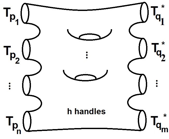
Figure 1: Genus $h-1$ surface with insertions of elements of the class algebra. A surface with $h=2$ is shown.

By cutting the path integral open, we can get two states. For example, the ket vector

$$\displaystyle|T_{p_{1}},T_{p_{2}},\cdots,T_{p_{n}}\rangle=\begin{gathered}\includegraphics[width=78.04842pt]{ket}\end{gathered}$$ (4.38)

belongs to $\hbox{Sym}^{k}({\cal H})$, the symmetric product of $k$ copies of ${\cal H}$. The ket vector is invariant under swapping the $T_{i}$s so that for example

$$\displaystyle|T_{p_{1}},T_{p_{2}},T_{p_{3}},\cdots,T_{p_{n}}\rangle=|T_{p_{2}},T_{p_{1}},T_{p_{3}},\cdots,T_{p_{n}}\rangle$$ (4.39)

This follows directly from the starting point (4.36). We can also define the bra vector

$$\displaystyle\langle T_{q_{1}}^{*},T_{q_{2}}^{*},\cdots,T_{q_{m}}^{*}|=\begin{gathered}\includegraphics[width=78.04842pt]{bra}\end{gathered}$$ (4.41)

which enjoys the same symmetry

$$\displaystyle\langle T_{q_{1}}^{*},T_{q_{2}}^{*},T_{q_{3}}^{*},\cdots,T_{q_{n}}^{*}|=\langle T_{q_{2}}^{*},T_{q_{1}}^{*},T_{q_{3}}^{*},\cdots,T_{q_{m}}^{*}|$$ (4.42)

The inner product of this bra and ket corresponds to the partition function

$$\displaystyle\langle T_{q_{1}}^{*},T_{q_{2}}^{*},\cdots,T_{q_{m}}^{*}|T_{p_{1}},T_{p_{2}},\cdots,T_{p_{n}}\rangle=Z_{\Sigma_{h,T_{p_{1}}\cdots T_{p_{n}}T_{q_{1}}^{*}\cdots T_{q_{m}}^{*}}}$$ (4.43)

We can define a set of commuting operators, which act as follows

$$\displaystyle\hat{T}_{a}|T_{p_{1}},T_{p_{2}},\cdots,T_{p_{n}}\rangle=|T_{p_{1}},T_{p_{2}},\cdots,T_{p_{n}},T_{a}\rangle$$ (4.44)

These operators commute thanks to the symmetry (4.39). These are the baby universe creation operators in this model [20, 24]. Any state in the Hilbert space can be obtained by acting on the “vacuum state” $|0\rangle$, which corresponds to the surface without any boundary circles. So, for example

$$\displaystyle|T_{p_{1}},T_{p_{2}},\cdots,T_{p_{k}}\rangle=\hat{T}_{p_{1}}\,\hat{T}_{p_{2}}\,\cdots\,\hat{T}_{p_{k}}|0\rangle$$ (4.45)

We also have

$$\displaystyle\langle T_{l_{1}}^{*},T_{l_{2}}^{*},\cdots,T_{l_{k}}^{*}|=\langle 0|\hat{T}_{l_{1}}^{\dagger}\,\hat{T}^{\dagger}_{l_{2}}\,\cdots\,\hat{T}^{\dagger}_{l_{k}}$$ (4.46)

The $T_{i}$s and the $T_{i}^{\dagger}$s commute, which is again a direct consequence of (4.36). This means that we can simultaneously diagonalize all of these operators. The simultaneous eigenkets are $R$ states $|R\rangle$ which obey

$$\displaystyle\hat{T}_{p}|R\rangle={\chi_{R}(T_{p})\over d_{R}}|R\rangle$$ (4.47)

i.e. the eigenvalues of the $\hat{T}_{p}$ operators are the normalized characters. These states are the analog of the $\alpha$-eigenstates introduced in [24]. Similarly

$$\displaystyle\langle R|\hat{T}^{\dagger}_{p}={\chi_{R}(T_{p}^{*})\over d_{R}}\langle R|$$ (4.48)

We will now show that the $G$-TQFT2 partition function can be interpreted as a sum over a classical ensemble of theories. The norm of the vacuum state is given by

$$\displaystyle\langle 0|0\rangle=Z_{\Sigma_{h}}=\sum_{R}\left({|G|^{2}\over d_{R}^{2}}\right)^{h-1}\equiv\mathfrak{z}$$ (4.49)

To get a correctly normalized distribution we should divide by the norm of the vacuum state. The partition function is

$$\displaystyle Z_{\Sigma_{h,T_{p_{1}}\cdots T_{p_{k}}T^{*}_{q_{1}}\cdots T^{*}_{q_{l}}}} = \langle\hat{T}^{\dagger}_{q_{1}}\cdots\hat{T}^{\dagger}_{q_{l}}\hat{T}_{p_{1}}\cdots\hat{T}_{p_{k}}\rangle$$ (4.50)

$$= \sum_{R}\left({|G|^{2}\over d_{R}^{2}}\right)^{h-1}{\chi_{R}(T_{p_{1}})\over d_{R}}\cdots{\chi_{R}(T_{p_{k}})\over d_{R}}{\chi_{R}(T_{q_{1}}^{*})\over d_{R}}\cdots{\chi_{R}(T_{q_{l}}^{*})\over d_{R}}$$ (4.51)

$$\equiv \mathfrak{z}\sum_{R}p_{R}{\chi_{R}(T_{p_{1}})\over d_{R}}\cdots{\chi_{R}(T_{p_{k}})\over d_{R}}{\chi_{R}(T_{q_{1}}^{*})\over d_{R}}\cdots{\chi_{R}(T_{q_{l}}^{*})\over d_{R}}$$ (4.52)

where in the last line we pulled out the normalization of the vacuum state and we have introduced the notation

$$\displaystyle p_{R}(h)={\left({|G|^{2}\over d_{R}^{2}}\right)^{h-1}\over\sum_{T}\left({|G|^{2}\over d_{T}^{2}}\right)^{h-1}}$$ (4.53)

It is obvious that

$$\displaystyle\sum_{R}p_{R}(h)=1$$ (4.54)

If we set $h=0$ we find that

$$\displaystyle p_{R}(h=0)={d_{R}^{2}\over|G|}$$ (4.55)

which is the Plancherel measure.

Notice that we can write the partition function (4.50) as follows

$$\displaystyle\sum_{R}p_{R}{\cal O}_{p_{1},p_{2},\cdots,p_{l};q_{1},\cdots,q_{l}}(R)$$ (4.56)

which illustrates the fact that we can interpret the partition function as computing observables in a classical ensemble of theories. This interpretation has been discussed in [20].

From the point of view discussed above the weight $p_{R}(h=0)$ is the normalized version of the weight $({|G|^{2}\over d_{R}^{2}})^{h-1}$ for the normalized characters in (4.50). We observed earlier that the Plancherel distribution can be understood in terms of the amplitude for transition from the vacumm to disc (4.8). Generalizing this observation, the partition function for genus $h$ with one boundary and with insertion of the central element $P_{R}$ at the boundary is given by

$$\displaystyle Z_{h,1,P_{R}}={1\over|G|}\delta(\Pi^{h}P_{R})=\left({|G|^{2}\over d_{R}^{2}}\right)^{h-1}$$ (4.57)

We can use the gluing relation (4.15) to write the partition function as a sum over $R$-sectors

$$Z_{\Sigma_{h,T_{p_{1}}\cdots T_{p_{k}}T^{*}_{q_{1}}\cdots T^{*}_{q_{l}}}}={1\over|G|}\delta(\Pi^{h}T_{p_{1}}\cdots T_{p_{k}}T_{q_{1}}^{*}\cdots T_{q_{l}}^{*})$$ (4.58)

$$=\sum_{R}\delta(\Pi^{h}P_{R}){|G|\over d_{R}^{2}}\delta(P_{R}T_{p_{1}}\cdots T_{p_{k}}T_{q_{1}}^{*}\cdots T_{q_{l}}^{*})$$ (4.59)

$$=\sum_{R}\left({1\over|G|}\delta(\Pi^{h}P_{R})\right){|G|^{2}\over d_{R}^{2}}\delta(P_{R}T_{p_{1}}\cdots T_{p_{k}}T_{q_{1}}^{*}\cdots T_{q_{l}}^{*})$$ (4.60)

This shows that the sum over $R$-sectors in (4.50) can be interpreted geometrically by cutting the genus $h$ transition surface from the in and out circles, along a circle which separates the handles from the in-out states. On this circle we insert a complete set of projectors $P_{R}$ which span ${\cal H}={\cal Z}(\mathbb{C}(G))$. The equality (LABEL:RexpGeom) is illustrated below :

$$\displaystyle\begin{gathered}\includegraphics[width=78.04842pt]{SummingPr1}\end{gathered}=\sum_{R}\,\,\,\begin{gathered}\includegraphics[width=112.73882pt]{SummingPr2}\end{gathered}$$ (4.63)

It is useful to note that a central role is played in the above discussion by the algebra ${\cal Z}(\mathbb{C}(G))$. We can define a topological quantum mechanics by taking as state space ${\cal H}={\cal Z}(\mathbb{C}(G))$. This state space is a complex vector space, but equipped with additional structures. It has an associative product. There is a map $\delta:{\cal H}\rightarrow\mathbb{C}$ which is defined by using the delta function on the group and extending to the group algebra (and its centre) by linearity. We can define an inner product

$$\displaystyle g(\sum_{g_{1}}a_{g_{1}}g_{1},\sum_{g_{2}}b_{g_{2}}g_{2})=\sum_{g_{1},g_{2}}(a_{g_{1}})^{*}b_{g_{2}}\delta(g_{1}g_{2}^{-1})$$ (4.64)

On the projector basis the inner product is

$$\displaystyle g(P_{R},P_{S})=\delta_{RS}{d_{R}^{2}\over|G|}$$ (4.65)

Thus the inner product is non-degenerate and ${\cal H}$ is indeed a Hilbert space. The transition probabilities considered earlier in this section are maps from

$$\displaystyle S^{n}({\cal H})\rightarrow S^{m}({\cal H})$$ (4.66)

defined using the algebra multiplication in ${\cal H}$ and the delta function map $\delta:{\cal H}\rightarrow{\cal H}$. The state spaces ${\cal H}$ and

$$\displaystyle\bigoplus_{n=0}^{\infty}S^{n}({\cal H})\equiv S^{\infty}({\cal H})$$ (4.67)

provide the complete framework for computing the amplitudes and probabilities considered and may be usefully thought of as defining a one-dimensional topological quantum mechanical system encoding amplitudes of $G$-TQFT2/$G$-CTST and holographically dual to the two-dimensional theory. The topological nature is reflected in the fact that we have not chosen a non-vanishing Hamiltonian to define a time evolution, and all the interesting amplitudes, probabilities and their inter-relations are encoded in the overlaps involving the interesting elements of ${\cal H}$ such as the conjugacy class observables $T_{p}$, the projectors $P_{R}$ and the handle creation operator $\Pi$. The baby-universe creation operators (4.44) are operators on $S^{\infty}({\cal H})$.

4.3 Probabilities in $G$-CTST

In $G$-CTST it is natural to consider the partition function that results if we sum over all possible $h$ values. The resulting partition function continues to have an interpretation as an ensemble average. If we sum over genera, then the norm of the ground state is

$$\displaystyle\langle 0|0\rangle=\sum_{h=0}^{\infty}Z_{\Sigma_{h}}g_{st}^{2h-2}=\sum_{h=0}^{\infty}\sum_{R}\left({|G|^{2}\over d_{R}^{2}}\right)^{h-1}g_{st}^{2h-2}$$ (4.68)

where $g_{st}$ is the string coupling. There is a sum over $h$ for each $R$, each of which looks like a geometric progression, with radius

$$\displaystyle r={|G|^{2}g_{st}^{2}\over d_{R}^{2}}$$ (4.69)

The sum over $h$ converges as long as

$$\displaystyle g_{st}^{2}<{d_{R}^{2}\over|G|^{2}}$$ (4.70)

Performing the geometric sum, we find

$$\displaystyle\langle 0|0\rangle=\sum_{R}{{d_{R}^{2}\over|G|^{2}g_{st}^{2}}\over 1-{|G|^{2}g_{st}^{2}\over d_{R}^{2}}}=\sum_{R}{d_{R}^{4}\over g_{st}^{2}|G|^{2}(d_{R}^{2}-|G|^{2}g_{st}^{2})}$$ (4.71)

Notice that the condition ensuring that the geometric sum converges also ensures that the norm of $\langle 0|0\rangle$ is positive.

The partition function is

$$\displaystyle Z_{\Sigma_{T_{p_{1}}\cdots T_{p_{n}}T_{q_{1}}^{*}\cdots T_{q_{m}}^{*}}} = \langle\hat{T}^{\dagger}_{q_{1}}\cdots\hat{T}^{\dagger}_{q_{m}}\hat{T}_{p_{1}}\cdots\hat{T}_{p_{n}}\rangle$$ (4.72)

$$= \sum_{R}\sum_{h=0}^{\infty}\left({|G|^{2}\over d_{R}^{2}}\right)^{h-1}{\chi_{R}(T_{p_{1}})\over d_{R}}\cdots{\chi_{R}(T_{p_{n}})\over d_{R}}{\chi_{R}(T_{q_{1}}^{*})\over d_{R}}\cdots{\chi_{R}(T_{q_{m}}^{*})\over d_{R}}$$ (4.73)

$$\equiv \mathfrak{z}\sum_{R}\sum_{h=0}^{\infty}p_{R}{\chi_{R}(T_{p_{1}})\over d_{R}}\cdots{\chi_{R}(T_{p_{n}})\over d_{R}}{\chi_{R}(T_{q_{1}}^{*})\over d_{R}}\cdots{\chi_{R}(T_{q_{m}}^{*})\over d_{R}}$$ (4.74)

where

$$\displaystyle p_{R}=\left(\sum_{T}{d_{T}^{4}\over g_{st}^{2}|G|^{2}(d_{T}^{2}-|G|^{2}g_{st}^{2})}\right)^{-1}{d_{R}^{4}\over g_{st}^{2}|G|^{2}(d_{R}^{2}-|G|^{2}g_{st}^{2})}$$ (4.75)

It is obvious that

$$\displaystyle\sum_{R}p_{R}=1$$ (4.76)

Again, we can write the partition function as

$$\displaystyle{Z_{\Sigma_{T_{p_{1}}\cdots T_{p_{k}}T_{q_{1}}^{*}\cdots T_{q_{l}}^{*}}}\over\langle 0|0\rangle}=\sum_{R}p_{R}\langle 0|\hat{T}^{\dagger}_{q_{1}}\cdots\hat{T}^{\dagger}_{q_{l}}\hat{T}_{p_{1}}\cdots\hat{T}_{p_{k}}|0\rangle$$ (4.77)

which illustrates the fact that we can interpret the partition function as computing observables in a classical ensemble of theories. As in section 4.2 the amplitudes and probabilities considered and their inter-relations can expressed within a topological quantum mechanics based on ${\cal H}$ and $S^{\infty}({\cal H})$.

5 S-duality for $G$-CTST

The calculations performed in sections 2 and 3 have established that $G$-CTST provides a construction of the dimensions $d_{R}$ and the characters of the irreducible representations of any finite group. These constructions are examples of Fourier transforms, valid for general groups, between representation theory data and group-combinatoric data. In this section we will show that the same methods can be used to give an interpretation for sums of positive powers of the dimensions of irreducible representations, including for example

$$\displaystyle\sum_{R}d_{R}^{4}$$ (5.1)

in terms of $G$-TQFT2 with defects, for any finite group $G$. Further, we will argue that this construction is intimately related to the S-duality transformation of $G$-CTST.

The group algebra $\mathbb{C}(G)$ has an inner product

$$\displaystyle\langle g_{1}|g_{2}\rangle=\delta(g_{1}g_{2}^{-1})$$ (5.2)

Consider the algebra

$$\displaystyle\mathbb{C}(G)\otimes\mathbb{C}(G)$$ (5.3)

There is an operator $X$ acting on the algebra as a projector, whose image has dimension $\sum_{R}d_{R}^{4}$. The projector $X$ is defined by

$$\displaystyle X=\sum_{R}P_{R}\otimes P_{R}\qquad P_{R}={d_{R}\over|G|}\sum_{g\in G}\chi_{R}(g)g^{-1}$$ (5.4)

Indeed, a straight forward computation gives

$$\displaystyle{\rm Tr}(X) = \sum_{g_{1},g_{2}\in G}\langle g_{1},g_{2}|X|g_{1},g_{2}\rangle$$ (5.5)

$$= \sum_{R}\sum_{g_{1},g_{2}}\delta(g_{1}^{-1}P_{R}g_{1})\delta(g_{2}^{-1}P_{R}g_{2})$$ (5.6)

$$= \sum_{R}|G|^{2}\delta(P_{R})\delta(P_{R})$$ (5.7)

$$= \sum_{R}d_{R}^{2}\sum_{g_{1}\in G}\chi_{R}(g_{1})\delta(g_{1}^{-1})\sum_{g_{2}\in G}\chi_{R}(g_{2})\delta(g_{2}^{-1})$$ (5.8)

$$= \sum_{R}d_{R}^{4}$$ (5.9)

providing a construction of the sum (5.1). This is a partition function on a product of two tori, each of which has a single boundary. To see this, note that the geometrical interpretation of the delta functions is as follows

$$\displaystyle\begin{gathered}\includegraphics[scale={0.4}]{deltadelta.jpg}\end{gathered}=\delta(g_{1}^{-1}P_{R}g_{1})\delta(g_{2}^{-1}P_{R}g_{2})$$ (5.11)

Summing over $g_{1}$ and $g_{2}$ closes the cylinders into tori

$$\sum_{R}\begin{gathered}\includegraphics[scale={0.4}]{torustorus.jpg}\end{gathered}=\sum_{R}\sum_{g_{1}}\delta(g_{1}^{-1}P_{R}g_{1})\sum_{g_{2}}\delta(g_{2}^{-1}P_{R}g_{2})=\sum_{R}d_{R}^{4}$$

A simple extension of the logic above can be used to give a formula for $\sum_{R}d_{R}^{2k}$ for any positive integer $k$. In this case the operator playing the role of $X$ is given by

$$\displaystyle\sum_{R}P_{R}\otimes P_{R}\otimes\cdots\otimes P_{R}$$ (5.12)

where there are $k$ factors in the tensor product.

There is an alternative description for $X$, which does not explicitly use the projectors $P_{R}$. We will give a description of this for the case where $G$ is symmetric group $S_{n}$, where known facts about the centre of ${\cal Z}(\mathbb{C}(S_{n}))$ allow a concrete discussion. We will make use of $T_{k}\in{\cal Z}(\mathbb{C}(S_{n}))$ given by summing all permutations with a single non-trivial cycle of length $k$. This alternative description follows by exploiting the fact that conjugacy classes labelled by partitions of $n$ provide a basis for the centre of the group algebra $\mathbb{C}(S_{n})$, denoted as ${\cal Z}(\mathbb{C}(S_{n}))$[50]. It turns out that a subset of these basis elements, those given by $T_{k}$ with $k\leq k_{*}(n)$, will generate ${\cal Z}(\mathbb{C}(S_{n}))$[50]. $k_{*}(n)$ is a (not explicitly known) function of $n$ whose form is determined by the degeneracies in the characters of $S_{n}$. The projectors $P_{R}$ associated with irreducible representations of $S_{n}$ also generate ${\cal Z}(\mathbb{C}(S_{n}))$, so it is not surprising that these two possibilities exist. The alternative formula for $X$ follows by noting that the null space of $H$

$$\displaystyle H=\sum_{k=1}^{k_{*}(n)}(T_{k}\otimes 1-1\otimes T_{k})$$ (5.13)

is the image of $X$. To see why this is the case, note that $T_{k}$ is in ${\cal Z}(\mathbb{C}(S_{n}))$, so that any state belonging to an irreducible representation $R$ is an eigenstate of $T_{k}$ with eigenvalue determined by $R$. If two states have the same eigenvalue for each $T_{k}$ with $k\leq k_{*}(n)$, they must belong to the same irrep. Thus, states in the null space of $H$ are sums of tensor products of states, where each term tensors pairs of states that belong to the same irrep. This is clearly equal to the image of $X$. In order to apply this construction of $X$ to general $G$-TQFT2, we need to develop the results analogous to those of [50] for other $G$, i.e. identify sets of generating conjugacy class sums for the centre ${\cal Z}(\mathbb{C}(G))$. These generating sets can be chosen to be appropriate sets of conjugacy bbc news classes with small sizes.

This completes the discussion of the construction problem for positive power sums of $d_{R}$. We now explain the relevance of these constructions to the S-dual of $G$-CTST. Consider the sum of genus $h$ $G$-TQFT2 partition functions weighted by powers of the string coupling, which defines the partition function $Z(g_{st})$ of $G$-CTST

$$Z(g_{st})=\sum_{h=0}^{\infty}g_{st}^{2h-2}Z_{\Sigma_{h}}=\sum_{h=0}^{\infty}g_{st}^{2h-2}\sum_{R}\left({|G|\over d_{R}}\right)^{2h-2}$$ (5.14)

$$=\sum_{R}{d_{R}^{2}\over|G|^{2}g_{st}^{2}}{1\over(1-g_{st}^{2}|G|^{2}/d_{R}^{2})}$$ (5.15)

Defining the dual string coupling $\tilde{g}_{st}=g_{st}^{-1}$ we have

$$\displaystyle Z(\tilde{g}_{st})=\sum_{R}{d_{R}^{4}\tilde{g}_{st}^{4}\over|G|^{2}(\tilde{g}_{st}^{2}d_{R}^{2}-|G|^{2})}$$ (5.16)

Studying this expression for small values of the dual coupling, defines a new $S$-dual expansion

$$\displaystyle Z(\tilde{g}_{st})=-\sum_{R}\sum_{n=0}^{\infty}\tilde{g}_{st}^{2+2n}{d_{R}^{4+2n}\over|G|^{4+2n}}\equiv\sum_{h}c_{h}\tilde{g}_{st}^{2h-2}$$ (5.17)

We see immediately that the dual partition function is written in terms of positive power sums of $d_{R}$ and that the genus of the surfaces being summed is

$$\displaystyle h=2+2n$$ (5.18)

For example, the term with $n=0$ is precisely the product of two tori described above.

5.1 Singularities of the partition function $G$-CTST as a function of string coupling

It is instructive to consider the analytic structure of $Z(g_{st}^{2})$ in the general complex $g_{st}^{2}$ plane and identify how group theoretic data appears in the singularity structure, i.e. the poles and residues of $Z(g_{st})$. To describe the simplest connections, it is convenient to consider the sum over genuses from $h=1$ to infinity, which we denoted as $Z_{1^{+}}(g_{st}^{2})$ We will find that this partition function has poles at $g_{st}^{2}=a_{R}^{-2}$ with $a_{R}\equiv{|G|\over d_{R}}$. It is possible for two distinct irreps to have the same dimension, so that we can have $a_{R}=a_{R^{\prime}}$, even when $R\neq R^{\prime}$. Denote the distinct values of $a_{R}^{-2}$ by $v_{i}$. The multiplicity $m_{v_{i}}$, of $v_{i}$ is given by the residue of the pole at $v_{i}$. These assertions are easily established with a simple computation

$$\displaystyle Z_{1^{+}}(g_{st}^{2}) = \sum_{h=1}^{\infty}g_{s}^{2h-2}Z_{h}=\sum_{h=1}^{\infty}\sum_{R}\left({|G|\over d_{R}}\right)^{2h-2}g_{s}^{2h-2}$$ (5.22)

$$=\sum_{R}{1\over(1-a_{R}^{2}g_{s}^{2})}$$

$$=\sum_{R}{a_{R}^{-2}\over(a_{R}^{-2}-g_{s}^{2})}$$

$$=\sum_{i=1}^{i_{*}}{-v_{i}^{2}m_{v_{i}}\over(g_{s}^{2}-v_{i}^{2})}$$

where there are a total of $i_{*}$ distinct $v_{i}$ values. Given the exact analytic form of the partition function, it is possible to generate a number of expansions, valid for different values of the coupling. The expansion shown on the first line of (5.22) above is for weak coupling, when the string coupling is smaller than all of the $v_{i}$. Notice that dimensions of irreps are raised to negative powers. The strong coupling expansion is valid when the string coupling is larger than all of the $v_{i}$. In this case, the expansion is

$$\displaystyle Z_{1^{+}}(g_{st}^{2}) = -\sum_{i=1}^{i_{*}}{v_{i}^{2}m_{v_{i}}\over(g_{s}^{2}-v_{i}^{2})}$$ (5.23)

$$= -\sum_{i=1}^{i_{*}}{v_{i}^{2}m_{v_{i}}\over g_{s}^{2}}\sum_{n=0}^{\infty}\left({v_{i}^{2}\over g_{s}^{2}}\right)^{n}$$ (5.25)

$$=-\sum_{R}{d_{R}^{2}\over|G|^{2}g_{s}^{2}}\sum_{n=0}^{\infty}\left({d_{R}^{2}\over|G|^{2}g_{s}^{2}}\right)^{n}$$

Notice that dimensions of irreps are now raised to positive powers.

There are other possibilities that generalize the weak coupling and strong coupling expansions. Choose the index $i$ so that the $v_{i}^{2}$ are ordered, i.e. $v_{1}^{2}<v_{2}^{2}<\cdots<v_{i_{*}}^{2}$. The more general expansions we could consider are obtained by choosing a value of the string coupling $g_{s}^{2}$ which is greater than $v_{1}^{2}$ but smaller than $v_{i_{*}}^{2}$. These more general expansions can not be written as power expansions in either $g_{s}^{2}$ or its inverse, but rather they are Laurent expansions in $g_{s}^{2}$. To develop these expansions, introduce the two sets $i_{<}$ and $i_{>}$ defined by

$$\displaystyle i_{<}=\{i|v_{i}^{2}<g_{s}^{2}\}\qquad i_{>}=\{i|v_{i}^{2}>g_{s}^{2}\}$$ (5.26)

The most general expansion of the partition function can now be written as

$$\displaystyle Z_{1^{+}}(g_{st}^{2})=\sum_{h=1}^{\infty}\sum_{i\in i_{<}}m_{v_{i}}v_{i}^{2-2h}g_{s}^{2h-2}-\sum_{h=1}^{\infty}\sum_{i\in i_{>}}m_{v_{i}}v_{i}^{2+2h}g_{s}^{-2-2h}$$ (5.27)

Note that when $i_{<}$ is empty we reproduce the strong coupling expansion of Section 5 and when $i_{>}$ is empty we reproduce the weak coupling expansion.

6 Finiteness relations in $G$-TQFT2

In this section, we describe relations between amplitudes in $G$-TQFT2/$G$-CTST due to the finiteness of $G$. The relations we describe are focused on amplitudes for closed surfaces and surfaces with boundary. They depend on the dimension of the centre ${\cal Z}(\mathbb{C}(G))$ which we denote as $K$. We have seen the key role played by matrices of size $K$ in the Sections 2 and 3 on the construction of representation theoretic data from group multiplication combinatorics shaped by the amplitudes. The algebra ${\cal Z}(\mathbb{C}(G))$ has also been prominent in the description of probability distributions associated with $G$-TQFT2 and $G$-CTST in section 4. In this section, we describe universal finite $K$ relations. We draw on some mathematical analogies between $G$-TQFT2 and the BPS sectors of $AdS_{5}/CFT_{4}$, based on the fact that the partition functions of $G$-TQFT2 are expressible in terms of traces of powers of a matrix. This allows us to define a simple inner product, such that the finite $K$ relations appear as null states in the inner product. The inner product contains a large $K$ factorization which fails when $1/K$ corrections are taken into account. The failure of factorization has a geometrical interpretation in terms of a mixing between surfaces with different numbers of connected components. We give a 2D topological field theory formulation of the inner product by coupling $G$-TQFT2 to TQFT2 based on symmetric group algebras. We describe this coupled toplogical field theory as $\mathbb{C}(G)\times(\mathbb{C}(S))_{\infty}$ TQFT2.

6.1 Finite $K$ relations from null states of an inner product

Pick a finite group $G$ and let $K$ be the number of conjugacy classes. It determines a matrix $X={\rm{Diag}}(|G|^{2}/d_{R}^{2})$ of size $K$. $G-TQFT2$ associates to a surface of genus $h$ the partition function

$$\displaystyle Z_{\Sigma_{h}}={\rm tr}X^{h-1}\equiv Z_{h}$$ (6.1)

A disconnected surface has a partition function which is a product over the connected components, e.g. with two components we

$$\displaystyle Z(\Sigma_{h_{1}}\times\Sigma_{h_{2}})={\rm tr}X^{h_{1}-1}{\rm tr}X^{h_{2}-1}$$ (6.2)

This can be computed by lattice TQFT2 on the two surfaces [17, 19].

The finite $K$ relations ensure that higher genus connected partition functions can be written in terms of linear combinations of partition functions for disconnected surfaces. This is a consequence of the Cayley Hamilton relations, which state that any matrix $X$ obeys its own eigenvalue equation. We have, using the elementary symmetric polynomials $e_{k}(X)$ described in section 2

$$\displaystyle X^{K}+\sum_{k=1}^{K}(-1)^{k}e_{k}(X)X^{K-k}=0$$ (6.3)

Multiply this with $X^{l}$ for any positive integer $l$

$$\displaystyle X^{K+l}+\sum_{k=1}^{K}(-1)^{k}e_{k}(X)X^{K-k+l}=0$$ (6.4)

Taking a trace on both sides, we have

$$\displaystyle{\rm tr}(X^{K+l})+\sum_{k=1}^{K}(-1)^{k}e_{k}(X){\rm tr}(X^{K-k+l})=0\,.$$ (6.5)

For $l=1$, this gives ${\rm tr}X^{K+1}$ as a linear combination of products of traces of lower powers of $X$ than the $K$’th power. Writing the elementary symmetric functions $e_{k}(X)$ in terms of traces of $X$ using (LABEL:ekformula), we obtain the trace relation

$$\displaystyle{\rm tr}X^{K+1}=\sum_{k=1}^{K}{\rm tr}X^{K-k+1}\sum_{p\vdash k}{(-1)^{1+\sum_{i}p_{i}}\over\prod_{i}i^{p_{i}}p_{i}!}\prod_{i}({\rm tr}X^{i})^{p_{i}}$$ (6.6)

For example if $K=3$ we have

$$\displaystyle{\rm tr}X^{4}={\rm tr}X{\rm tr}X^{3}-{1\over 2}({\rm tr}X^{2}+({\rm tr}X)^{2}){\rm tr}X^{2}+{1\over 6}(2{\rm tr}X^{3}+3{\rm tr}X^{2}{\rm tr}X+({\rm tr}X)^{3}){\rm tr}X$$ (6.7)

The relation (6.75) implies that the genus $K+2$ partition function $Z_{K+2}={\rm tr}(X^{K+1})$ can be expressed in terms of products of smaller genus partition functions

$$\displaystyle Z_{K+2}=\sum_{k=1}^{K}Z_{K-k+2}\sum_{p\vdash k}{(-1)^{1+\sum_{i}p_{i}}\over\prod_{i}i^{p_{i}}p_{i}!}\prod_{i}(Z_{i+1})^{p_{i}}$$ (6.8)

To obtain this result we have used the expression for the partition functions in terms of traces.

These equations raise the interesting question of how to describe the finite $K$ relations among $G$-TQFT2 amplitudes in generality. The matrix form of the partition function $Z_{h}={\rm tr}(X^{h-1})$ relates this question to the description of finite $N$ effects in the AdS/CFT correspondence [51, 53, 52], specifically the half-BPS sector of string theory in $AdS_{5}\times S^{5}$ which corresponds to ${\cal N}=4$ super-Yang-Mills theory with $U(N)$ gauge group. Such finite $N$ effects are associated with the very rich physics of the stringy exclusion principle and giant gravitons [54, 27]. The half-BPS states of ${\cal N}=4$ SYM for $U(N)$ gauge group correspond (by the operator-state correspondence of CFT) to multi-traces of a complex matrix $Z$. An orthogonal basis for these states using the free field inner product in the $U(N)$ theory is labelled by Young diagrams [30]. If we consider gauge invariant states (multi-traces) of dimension $n$, i.e. containing $n$ copies of $Z$, in the range $n>N$, there is subspace of the vector space of these trace operators which vanishes due to finite $N$ relations (Cayley-Hamilton relations discussed above). A linear basis for these vanishing states is labelled by Young diagrams $R$ with first column of length greater than $N$. These are null states for the $N$-dependent inner product for multi-trace structures which comes from free field $U(N)$ theory.

In order to answer the question of a systematic description of finite $K$ relations for a group $G$ with $K$ conjugacy classes, using the above technical perspectives from the mathematics of the stringy exclusion principle in AdS/CFT, it is convenient to introduce an abstract polynomial algebra ${\cal P}(\omega_{1},\omega_{2},\cdots)$. This is a vector space over $\mathbb{C}$. $\omega_{k}$ corresponds to a topological surface of genus $k+1$. We have a generator $\omega_{1}$ for a surface of genus $2$, a generator $\omega_{2}$ for a surface of genus $3$ etc. A monomial $\omega_{1}^{k_{1}}\omega_{2}^{k_{2}}\cdots\omega_{l}^{k_{l}}$ corresponds to a disjoint union of $k_{1}$ genus two surfaces, $k_{2}$ genus $3$ surfaces, up to $k_{l}$ genus $l+1$ surfaces. These finite monomials form a basis for the vector space ${\cal P}(\omega_{1},\omega_{2},\cdots)$. The vector space ${\cal P}(\omega_{i})$ is endowed with a product defined as the product of these monomials. $G$-TQFT2 associates to the monomial

$$\hbox{ $G$-TQFT2 }:\omega_{1}^{k_{1}}\omega_{2}^{k_{2}}\cdots\omega_{l}^{k_{l}}\rightarrow\Sigma_{2}^{\times k_{1}}\times\Sigma_{3}^{\times k_{2}}\cdots\Sigma_{l+1}^{k_{l}}\rightarrow({\rm tr}X)^{k_{1}}({\rm tr}X^{2})^{k_{2}}\cdots({\rm tr}X^{l})^{k_{l}}$$ (6.9)

where $X$ is a $K\times K$ diagonal matrix, with entries labelled by irreps $R$ of $G$, and taking values ${|G|\over d_{R}}$. $AdS_{5}/CFT_{4}$ associates to the same monomials half-BPS states corresponding to matrix traces

$$\displaystyle\hbox{AdS${}_{5}$/CFT${}_{4}$ }:\omega_{1}^{k_{1}}\omega_{2}^{k_{2}}\cdots\omega_{l}^{k_{l}}\rightarrow({\rm tr}Z)^{k_{1}}({\rm tr}Z^{2})^{k_{2}}\cdots({\rm tr}Z^{l})^{k_{l}}$$ (6.11)

where $Z=X_{1}+iX_{2}$ and $X_{1},X_{2}$ are two of the $6$ hermitian matrices of $U(N)$ ${\cal N}=4$ SYM. The parameter $N$ in the AdS5/CFT4 context is analogous to $K$ in the case of $G$-TQFT2.

The computation of 2-point functions of general holomorphic trace of dimension $n$ in ${\cal N}=4$ SYM with another general anti-homolomorphic trace defines an inner product on the space of traces. The outcome of the computation can be expressed using permutations in the symmetric group $S_{n}$. Consider the 2-point function

$$\displaystyle\langle({\rm tr}Z)^{p_{1}}({\rm tr}Z^{2})^{p_{2}}\cdots({\rm tr}Z^{l})^{p_{l}}({\rm tr}Z^{\dagger})^{q_{1}}({\rm tr}(Z^{\dagger})^{2})^{q_{2}}\cdots({\rm tr}(Z^{\dagger})^{l})^{q_{m}}\rangle$$ (6.12)

where the holomorphic operator has a trace structure specified by the exponents $(p_{1},p_{2},\cdots p_{l})\equiv p$, and the anti-holomorphic operator has a trace structure specified by $(q_{1},q_{2},\cdots,q_{m})\equiv q$. For fixed dimension $n$, we have $n=\sum_{i}ip_{i}=\sum_{i}iq_{i}$. $p$ and $q$ are partitions of $n$, which also correspond to conjugacy classes of $S_{n}$. The 2-point function determines the inner product [30]

$$\langle({\rm tr}Z)^{p_{1}}({\rm tr}Z^{2})^{p_{2}}\cdots({\rm tr}Z^{l})^{p_{l}}({\rm tr}Z^{\dagger})^{q_{1}}({\rm tr}(Z^{\dagger})^{2})^{q_{2}}\cdots({\rm tr}(Z^{\dagger})^{l})^{q_{m}}\rangle$$ (6.13)

$$={n!\over|{\cal C}_{p}||{\cal C}_{q}|}\sum_{\sigma_{1}\in{\cal C}_{p}}\sum_{\sigma_{2}\in{\cal C}_{q}}\sum_{\sigma_{3}\in S_{n}}\delta(\sigma_{1}\sigma_{2}\sigma_{3})N^{C_{\sigma_{3}}}$$ (6.14)

where $C_{\sigma_{3}}$ is the umber of cycles in $\sigma_{3}$. The Schur-basis of gauge invariant operators are labelled by Young diagrams $Y$ with $n$ boxes

$$\displaystyle\chi^{Y}(Z)={1\over n!}\sum_{\sigma\in S_{n}}\chi^{Y}(\sigma){\cal O}_{\sigma}(Z)$$ (6.15)

where

$$\displaystyle{\cal O}_{\sigma}(Z)=Z^{i_{1}}_{i_{\sigma(1)}}\cdots Z^{i_{n}}_{\sigma(n)}$$ (6.16)

The two point function in the Schur basis is given by

$$\displaystyle\langle\chi^{Y_{1}}(Z)\chi^{Y_{2}}(Z^{\dagger})\rangle=\delta^{Y_{1},Y_{2}}f_{Y_{1}}$$ (6.17)

The normalization factor $f_{Y}$ for a Young diagram is a polynomial in $N$ equal to

$$\displaystyle f_{Y}=\prod_{(i,j)}(N-i+j)$$ (6.18)

where $(i,j)$ are row and column labels of the boxes in the Young diagram $Y$. The norm of all Young diagram states with $Y$ having more than $N$ rows vanishes and in fact the polynomials $\chi^{Y}(Z)$ are identically zero for $Z$ of size $N$. Thus the inner product (LABEL:HBPSIP) for trace structures encodes finite $N$ relations on traces in the form of null states for an inner product.

We give the algebra ${\cal P}(\omega_{i})$ an inner product depending on a parameter $K$ of the form familiar from the matrix combinatorics (LABEL:HBPSIP) of the half-BPS sector in AdS5/CFT4:

$$\displaystyle\langle\omega_{1}^{p_{1}}\omega_{2}^{p_{2}}\cdots|\omega_{1}^{q_{1}}\omega_{2}^{q_{2}}\cdots\rangle={n!\over|{\cal C}_{p}||{\cal C}_{q}|}\sum_{\sigma_{1}\in{\cal C}_{p}}\sum_{\sigma_{2}\in{\cal C}_{q}}\sum_{\sigma_{3}\in S_{n}}\delta(\sigma_{1}\sigma_{2}\sigma_{3})K^{C_{\sigma_{3}}}$$ (6.19)

With this inner product, all the finite $K$ relations are null states and can be expressed in terms of Schur Polynomials of $X$. Using the $G$-TQFT2 map, this corresponds to an inner product between surfaces $\prod_{i}\Sigma_{i+1}^{\times p_{i}}$ and $\prod_{i}\Sigma_{i+1}^{q_{i}}$, with $n=\sum_{i}ip_{i}=\sum_{i}iq_{i}$. The Schur basis for algebra ${\cal P}(\omega_{i})$ is obtained by replacing

$$\displaystyle\chi^{Y}(X)={1\over n!}\sum_{p\vdash n}{1\over|{\cal C}_{p}|}\chi^{Y}(T_{p})\prod_{i}{\rm tr}(X^{i})^{p_{i}}\rightarrow\chi^{Y}(\omega)={1\over n!}\sum_{p\vdash n}{1\over|{\cal C}_{p}|}\chi^{Y}(T_{p})\prod_{i}(\omega^{i})^{p_{i}}$$ (6.20)

The inner product in the Schur basis is

$$\displaystyle\langle\chi^{Y_{1}}(\omega)|\chi^{Y_{2}}(\omega)\rangle=f_{Y_{1}}\delta^{Y_{1}Y_{2}}$$ (6.21)

Factorization and $1/K$ corrections to factorization: The inner product (6.19) factorizes in the leading large $K$ limit. In this limit the dominant term comes from the case where $\sigma_{3}$ has the maximum number of cycles, i.e. $C_{\sigma_{3}}=n$ and $\sigma_{3}$ is the identity permutation. In this case, ${\cal C}_{p}={\cal C}_{q}$ and the inner product is non-zero only when $p$ and $q$ describe the same trace structure. At subleading orders in $K$, other permutations $\sigma_{3}$ contribute and the precise departures from $p=q$ are encoded in permutation products. In the $G$-TQFT2 interpretation of the inner product, the factorization means that different monomials in $\omega_{i}$, which correspond to surfaces with different numbers of connected components, are orthogonal at large $K$ and there are corrections to this factorization at sub-leading orders in $1/K$. In the context of AdS5/CFT4, the departures from factorization formed an important argument in guiding the identification of CFT operators for giant gravitons [31, 30].

The inner product we have considered is not the unique inner product that is compatible with the finite K relations. Other possible inner products are determined by Casimirs as follows

$$\displaystyle\langle\omega_{1}^{p_{1}}\omega_{2}^{p_{2}}\cdots|\omega_{1}^{q_{1}}\omega_{2}^{q_{2}}\cdots\rangle={n!\over|{\cal C}_{p}||{\cal C}_{q}|}\sum_{\sigma_{1}\in{\cal C}_{p}}\sum_{\sigma_{2}\in{\cal C}_{q}}\sum_{\sigma_{3}\in S_{n}}\delta(\sigma_{1}\sigma_{2}\sigma_{3}C)K^{C_{\sigma_{3}}}$$ (6.22)

We have inserted a Casimir element $C$ for $U(K)$ - expressed in terms of the group algebra of $S_{n}$. The existence of this map relies on Schur-Weyl duality and plays an important role in the string theory of 2D Yang Mills theory [56, 57, 58] as well as AdS5/CFT4 [49, 50].

This will still be diagonal in the Schur basis and would give a different normalisation of the 2-point function, modified by presence of the Casimir. The 2-point function in the Schur basis is now

$$\displaystyle\langle\chi^{Y_{1}}(\omega)|\chi^{Y_{2}}(\omega)\rangle=f_{Y_{1}}{\chi^{Y_{1}}(C)\over d_{Y_{1}}}$$ (6.23)

6.2 Finiteness relations and $\mathbb{C}(G)\times(\mathbb{C}(S))_{\infty}$ two dimensional topological field theory

In the above discussion, we have found it useful to introduce a simple inner product for a polynomial algebra of Riemann surfaces, which captures the finite $K$ relations $G$-TQFT2. The simplest inner product coincides with an inner product we have seen in the half-BPS sector of $N=4$ SYM, but variations of the inner product which also capture the finite $K$ relations are also described. A natural question is: how do we interpret these inner products as a construction within Dijkgraaf-Witten theory? Closely related to Dijkgraaf-Witten theory is the open-closed topological field theory developed by Moore and Segal [25]. In [25] the amplitudes of Dijkgraaf-Witten theory for closed surfaces and surfaces with boundary are interpreted in terms of the centre of the associative algebra $\mathbb{C}(G)$ which is equipped with a trace map which is the trace in the regular representation. There is also an extension to open strings which uses $\mathbb{C}(G)$ and not just its centre, but we will not make extensive use of the open string sector in this paper.

Consider the central element $\widehat{Y}_{h}\in{\cal Z}(\mathbb{C}(G))$

$$\displaystyle\widehat{Y}_{h}=\Pi^{h}$$ (6.24)

where

$$\displaystyle\Pi=\sum_{g_{1},g_{2}\in G}g_{1}g_{2}g_{1}^{-1}g_{2}^{-1}=\sum_{R}{|G|^{2}\over d_{R}^{2}}P_{R}$$ (6.25)

As discussed in section 4 $\Pi$ can be viewed as a handle-creation operator. In terms of the handle creation operator, the partition function for genus $h$ is

$$\displaystyle Z_{\Sigma_{h}}={1\over|G|}\delta(\widehat{Y}_{h})$$ (6.26)

This partition function also has an expansion, in terms of Young diagrams, as

$$\displaystyle Z_{\Sigma_{h}}=\sum_{R}\left({|G|\over d_{R}}\right)^{2(h-1)}={\rm tr}X^{h-1}$$ (6.27)

where

$$\displaystyle X={\rm{Diag}}\left({|G|^{2}\over d_{R}^{2}}\right)$$ (6.28)

The handle creation operator $\widehat{Y}_{h}$ has an expansion in terms of central class elements $T_{\mu}$ as follows

$$\displaystyle\widehat{Y}_{h} =\sum_{p}\delta(\widehat{Y}_{h}T_{p}){T_{p}^{\prime}\over{|{\cal C}_{p}|}}$$ (6.30)

$$=\sum_{p}\left({1\over|G|}\delta(Y_{h}T_{p})\right)~{}T_{p}^{\prime}~{}|{\hbox{Sym}~{}{\cal C}_{p}}|$$

An important consequence of this expansion is that it can be used to develop an instructive geometrical interpretation. The delta function is proportional to the partition function on a genus $h$ surface with a disc removed, $\Sigma_{h,1}$, with

$$\displaystyle Z_{\Sigma_{h,1};T_{p}}={1\over|G|}\delta(\hat{Y}_{h}T_{p})$$ (6.31)

The cylinder partition function defines an inner product

$$\displaystyle Z_{cyl}(T_{p},T_{q})={1\over|G|}\delta(T_{p}T_{q})=\delta_{{\cal C}_{p},{\cal C}_{q^{\prime}}}{|\hbox{Sym}({\cal C}_{p})|\over|G|}=\delta_{{\cal C}_{p},{\cal C}_{q^{\prime}}}{1\over|{\cal C}_{p}|}$$ (6.32)

Given the expansion (6.30), we can interpret $\widehat{Y}_{h}$, as a state in the Hilbert space ${\cal Z}(\mathbb{C}(G))$ corresponding to the genus $h$ surface with one boundary. Recalling that

$$\displaystyle{1\over|G|}\delta(\cdot)$$ (6.33)

is the function on ${\cal Z}(\mathbb{C}(G))$ given by disc partition function, we can interpret (6.26) as the gluing of the disc to the genus $h$ surface minus a hole, as illustrated below

$$\qquad\Pi=\sum_{g_{1},g_{2}\in G}g_{1}g_{2}g_{1}^{-1}g_{2}^{-1}$$ (6.34)

$$\begin{gathered}\includegraphics[width=130.08731pt]{hhandles1}\end{gathered}\qquad \rightarrow \qquad\widehat{Y}_{h}=\Pi^{h}\in{\cal Z}(\mathbb{C}(G))$$ (6.36)

$$\left({\cal Z}(\mathbb{C}(G))\right)^{*}\ni{1\over|G|}\delta(\cdot)\qquad \leftarrow \qquad\begin{gathered}\includegraphics[width=15.17828pt]{hhandles2}\end{gathered}$$ (6.38)

$$\begin{gathered}\includegraphics[width=130.08731pt]{hhandles3}\end{gathered}\qquad \rightarrow \qquad\begin{gathered}\includegraphics[width=130.08731pt]{hhandles4}\end{gathered}$$ (6.41)

$${1\over|G|}\delta(\widehat{Y}_{h})\qquad = \qquad Z(\Sigma_{h})$$ (6.42)

Developing the above discussion for a disconnected surface $\Sigma_{h_{1}}\times\Sigma_{h_{2}}\times\cdots\Sigma_{h_{L}}$ we find

$$\displaystyle Z_{\Sigma_{h_{1}}\times\Sigma_{h_{2}}\times\cdots\times\Sigma_{h_{L}}} = Z_{\Sigma_{h_{1}}}Z_{\Sigma_{h_{2}}}\cdots Z_{\Sigma_{h_{L}}}$$ (6.43)

$$= \left({1\over|G|}\delta\otimes{1\over|G|}\delta\otimes\cdots\otimes{1\over|G|}\delta\right)\left(\widehat{Y}_{h_{1}}\otimes\cdots\otimes\widehat{Y}_{h_{L}}\right)$$ (6.44)

This has the interpretation of gluing $k$ discs to $k$ surfaces of genera $h_{1},h_{2},\cdots,h_{k}$, each with a disc removed. The cut-and-paste operation produces the partition function from an element of $({\cal Z}(\mathbb{C}(G)))^{\otimes L}$ corresponding to an element of $({\cal Z}(\mathbb{C}(G)))^{*\otimes L}$. Diagrammatically, (6.44) can be represented as

$$\displaystyle\begin{array}[]{cccc}\begin{gathered}\includegraphics[width=13.00806pt]{hhandles}\end{gathered}&\begin{gathered}\includegraphics[width=130.08731pt]{h1handles}\end{gathered}&&\begin{gathered}\includegraphics[width=130.08731pt]{hh1handles}\end{gathered}\\ \begin{gathered}\includegraphics[width=13.00806pt]{hhandles}\end{gathered}&\begin{gathered}\includegraphics[width=130.08731pt]{h2handles}\end{gathered}&\longrightarrow&\begin{gathered}\includegraphics[width=130.08731pt]{hh2handles}\end{gathered}\\ \vdots&\vdots&\vdots&\vdots\\ \begin{gathered}\includegraphics[width=13.00806pt]{hhandles}\end{gathered}&\begin{gathered}\includegraphics[width=130.08731pt]{hkhandles}\end{gathered}&&\begin{gathered}\includegraphics[width=130.08731pt]{hhkhandles}\end{gathered}\\ {1\over|G|}\delta\otimes{1\over|G|}\delta\cdots\otimes{1\over|G|}\delta&\Pi^{h_{1}}\otimes\Pi^{h_{2}}\cdots\otimes\Pi^{h_{k}}&\longrightarrow&{1\over|G|^{k}}\delta(\Pi^{h_{1}})\cdots\delta(\Pi^{h_{1}})\end{array}$$ (6.59)

We have described an inner product for disconnected surfaces which accounts for the finite $K$ relations. This used symmetric groups $S_{n}$ for varying $n$, which is equal to the number of connected components in the surface being considered. Note that the formula for the inner product is itself given in terms of a delta function on the group algebra $\mathbb{C}(S_{n})$, which is suggestive of a permutation-TQFT2 interpretation of the inner product. The link between the combinatorics and correlators of $U(N)$ gauge theories, as well as theories involving products of $U(N_{a})$, with symmetric group TQFT2 has been studied systematically in [55, 59]. Building on these results, we show here how the inner product (6.19) for $G$-TQFT2 amplitudes can be given a geometrical interpretation by coupling the ${\cal Z}(\mathbb{C}(G))$ theory to a theory based on the algebra

$$\displaystyle\bigoplus_{n=0}^{\infty}(\mathbb{C}(S_{n}))$$ (6.60)

We will call this algebra $(\mathbb{C}S)_{\infty}$. The construction we describe is based on TQFT2 for the algebra

$$\displaystyle{\cal Z}(\mathbb{C}(G))\otimes(\mathbb{C}S)_{\infty}$$ (6.61)

The first important ingredient in the construction of this theory is a cylinder which maps central elements in ${\cal Z}(\mathbb{C}(G))$ to permutations $\Pi^{h}\rightarrow(1,...,h-1)$.

Consider the composition

$$\displaystyle\begin{gathered}\includegraphics[width=130.08731pt]{cylindertransition}\end{gathered}$$ (6.63)

The cylinder is a transition amplitude that takes in $\Pi^{h_{1}}$ and produces a permutation

$$\displaystyle\begin{gathered}\includegraphics[width=130.08731pt]{cylinder}\end{gathered}$$ (6.65)

This defines a transition between $\Pi^{h_{1}}\in{\cal Z}(\mathbb{C}(G))$ and a permutation. Thus, the cylinder is something that is defined in ${\cal Z}(\mathbb{C}(G))\otimes(\mathbb{C}S)_{\infty}$.

The formulae developed above can be used to given a diagrammatic interpretation to the inner product

$$\langle{\rm tr}(X^{h_{1}-1}){\rm tr}(X^{h_{2}-1})\cdots{\rm tr}(X^{h_{k}-1}){\rm tr}(X^{h_{1}^{\prime}-1}){\rm tr}(X^{h_{2}^{\prime}-1})\cdots{\rm tr}(X^{h_{l}^{\prime}-1})\rangle$$ (6.66)

$$={n!\over|C_{h_{1},\cdots,h_{k}}||C_{h_{1}^{\prime},\cdots,h_{l}^{\prime}}|}\sum_{\sigma_{1}\in C_{h_{1}h_{2}\cdots h_{k}}}\sum_{\sigma_{2}\in C_{h_{1}^{\prime}h_{2}^{\prime}\cdots h_{l}^{\prime}}}\sum_{\sigma_{3}\in S_{\sum_{i}h_{i}}}\delta(\sigma_{1}\sigma_{2}\sigma_{3})K^{C_{\sigma_{3}}}$$ (6.67)

On the RHS above the notation $C_{a_{1}a_{2}\cdots a_{l}}$ stands for the conjugacy class of permutations with cycle lengths given by $a_{1}-1,a_{2}-1,\cdots,a_{l}-1$. The above inner product is non-zero if and only if $\sum_{i}(h_{i}-1)=\sum_{i}(h_{i}^{\prime}-1)$. The partition function of the three holed sphere in $S_{n}$ TQFT2 of flat bundles, with boundary permutations $\sigma_{1},\sigma_{2},\sigma_{3}$ is

$$\displaystyle\begin{gathered}\includegraphics[width=86.72267pt]{threeholesphere.jpg}\end{gathered}=\sum_{\gamma_{1},\gamma_{2}}\delta(\gamma_{1}\sigma_{1}\gamma_{1}^{-1}\gamma_{2}\sigma_{2}\gamma_{2}^{-1}\sigma_{3}^{-1})$$ (6.70)

ensures that $\sigma_{3}$ lies in the product of the conjugacy class of $[\sigma_{1}]$ and the conjugacy class $[\sigma_{2}]$. By introducing a unit defect as in [55] we have

$$\displaystyle\begin{gathered}\includegraphics[width=86.72267pt]{threeholespheredefect.jpg}\end{gathered}=\delta(\sigma_{1}\sigma_{2}\sigma_{3}^{-1})$$ (6.72)

we set $\sigma_{3}=\sigma_{1}\sigma_{2}$. The inner product (6.67) can now be expressed in terms of diagrams.

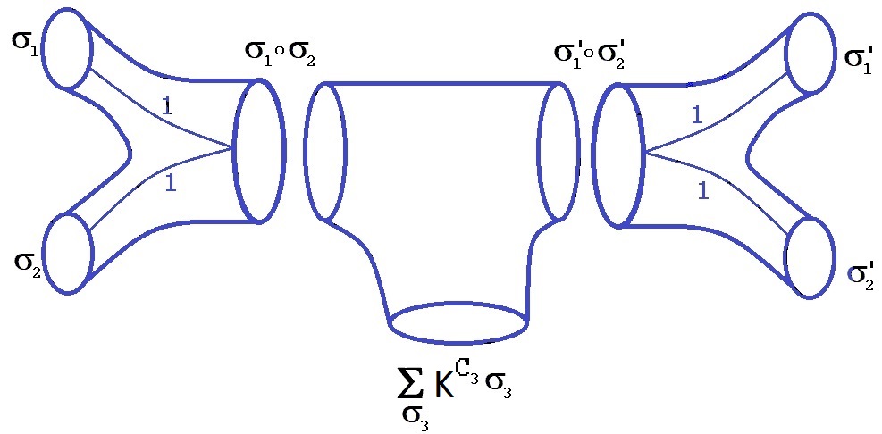
Figure 2: The interpretation of the inner product (6.74) in terms of diagrams. Here $\sigma_{1}=(1,2,\cdots,h_{1}-1)$, $\sigma_{2}=(h_{1},h_{1}+1,\cdots,h_{2}-2)$ and $\sigma_{1}\circ\sigma_{2}=(1,2,\cdots,h_{1}-1)(h_{1},h_{1}+1,\cdots,h_{2}-2)$. There are similar formulas for the primed permutations. The unit defect ensures that $\sigma_{1}\circ\sigma_{2}$ is a specific permutation and not a sum over a conjugacy class. $C_{3}$ is the number of cycles in $\sigma_{3}$ and $\sigma\circ\psi$ is the outer products of permutations $\sigma$ and $\psi$.

For clarity and because the generalization is immediate, consider the simpler formula

$$\displaystyle\langle{\rm tr}(X^{h_{1}-1}){\rm tr}(X^{h_{2}-1}){\rm tr}(X^{h_{1}^{\prime}-1}){\rm tr}(X^{h_{2}^{\prime}-1}))\rangle={n!\over|C_{h_{1},h_{2}}||C_{h_{1}^{\prime},h_{2}^{\prime}}|}\sum_{\sigma_{1}\in C_{h_{1}h_{2}}}\sum_{\sigma_{2}\in C_{h_{1}^{\prime}h_{2}^{\prime}}}\sum_{\sigma_{3}\in S_{\sum_{i}(h_{i}-1)}}\delta(\sigma_{1}\sigma_{2}\sigma_{3})K^{C_{\sigma_{3}}}$$ (6.73)

(6.74)

In terms of diagrams the formula (6.74) is displayed in Figure 2. The inner product is non-vanishing if and only if $h_{1}+h_{2}=h_{1}^{\prime}+h_{2}^{\prime}$. An more complete picture incuding the coupling between the $G$-TQFT2 and the symmetric group sector ( using the cylinder (6.65)) to write the inner product in terms of the TFT of the $(\mathbb{C}S)_{\infty}\otimes{\cal Z}(\mathbb{C}(G))$ algebra. This provides an interpretation for the inner product as an amplitude on a 2-complex, as given in Figure 3.

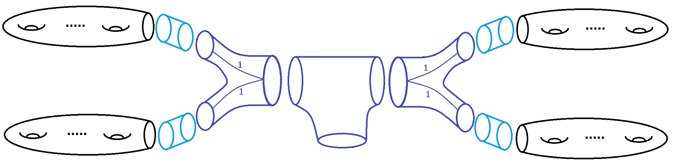
Figure 3: The interpretation of the inner product (6.74) in terms of diagrams.

6.3 Extensions of the finiteness discussion for closed surfaces

The discussion of the last subsection has related high genus surfaces without boundaries to disjoint unions of lower genus surfaces, again without boundaries. In this section we generalize this discussion first to surfaces with boundaries but fixed genus $h=1$, which involves the matrix $X_{p}$, and then to surfaces that have both multiple boundaries and any genus, which involves the pair $X,X_{p}$.

6.3.1 One-matrix finite $K$ relations for $X_{p}$

By using the matrix $X$ above, we have described relations between high genus surfaces and disjoint unions of lower genus surfaces. Similar relations hold for $X_{p}$, where $p$ is a conjugacy class. This will relate $trX_{p}^{K+1}$ with products of lower traces. Recalling (3.7) in Section 3 the LHS is the partition function of a surface of one with $K+1$ holes each carrying the conjugacy class $p$. The RHS is for disjoint unions of genus one but with fewer boundaries. The trace relation (6.75), expressed in terms of the matrix $X_{p}$ of normalized characters for a conjugacy class $p$, is

$$\displaystyle{\rm tr}X_{p}^{K+1}=\sum_{k=1}^{K}{\rm tr}X_{p}^{K-k+1}\sum_{p\vdash k}{(-1)^{1+\sum_{i}p_{i}}\over\prod_{i}i^{p_{i}}p_{i}!}\prod_{i}({\rm tr}X_{p}^{i})^{p_{i}}$$ (6.75)

Since these traces are partition functions for surfaces with boundary conditions labelled by $p$, we have a relation

$$\displaystyle Z(\Sigma_{h=1;{\cal C}_{p}^{\times(K+1)}})=\sum_{k=1}^{K}Z(\Sigma_{h=1;{\cal C}_{p}^{\times(K-k+1)}})\sum_{p\vdash k}{(-1)^{1+\sum_{i}p_{i}}\over\prod_{i}i^{p_{i}}p_{i}!}\prod_{i}(Z(\Sigma_{h=1;{\cal C}_{p}^{\times(i)}}))^{p_{i}}$$ (6.76)

6.3.2 2-Matrix finite $K$ relations

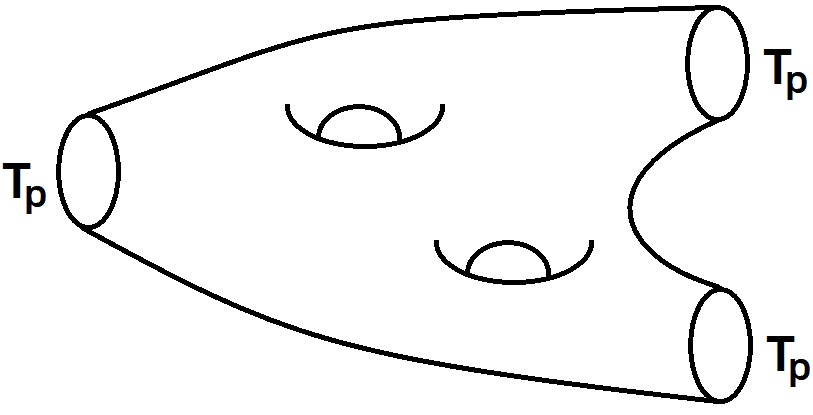
Figure 4: The surface shown has genus $h=2$ with $k=3$ boundaries.

The partition function for a genus $h$ surface, with $k$ one-dimensional boundaries, each having the boundary condition that the holonomy around the boundary circle is in the conjugacy class ${\cal C}_{p}$ is given by

$$\displaystyle Z(\Sigma_{h;{\cal C}_{p},\cdots,{\cal C}_{p}})=Z(\Sigma_{h;{\cal C}_{p}^{\times k}})={\rm tr}(X^{h-1}X_{p}^{k})$$ (6.77)

where $X$ and $X_{p}$ are commuting diagonal matrices, with diagonal entries labelled by irreducible representations $R$ of $G$

$$X={\rm{Diag}}\left({|G|\over d_{R}}\right)$$ (6.78)

$$X_{p}={\rm{Diag}}\left({\chi^{R}(T_{p})\over d_{R}}\right)$$ (6.79)

The finiteness of $K$ means that partition functions at high $h$ and high $k$ are expressible in terms of products of traces of lower powers. For example consider

$$\displaystyle Z(\Sigma_{h=K+1;{\cal C}_{p}^{\times K+1}})={\rm tr}((XX_{p})^{K+1})$$ (6.80)

The equation (6.75) with $X_{p}\rightarrow XX_{p}$ implies a finite $K$ relation relating this boundary partition function to lower boundary partition functions as follows

$$\displaystyle Z(\Sigma_{h=K+1;{\cal C}_{p}^{\times(K+1)}})=\sum_{k=1}^{K}Z(\Sigma_{h=K-k+1;{\cal C}_{p}^{\times(K-k+1)}})\sum_{p\vdash k}{(-1)^{1+\sum_{i}p_{i}}\over\prod_{i}i^{p_{i}}p_{i}!}\prod_{i}Z(\Sigma_{h=i;{\cal C}_{p}^{\times i}})^{p_{i}}$$ (6.81)

The systematic finite $K$ relations can be obtained using multi-symmetric functions. For ease of notation, we will write $X_{p}=Y$, so we are dealing with traces of two commuting matrices $X,Y$. There is a trace basis of functions of these two diagonal matrices, which is labelled by a sequence $[{\bf q}]\equiv[(q_{11},q_{12}),(q_{21},q_{22}),\cdots,(q_{M1},q_{M2})]$ with $q_{i1},q_{i2}\in\mathbb{N}_{0}$ where $\mathbb{N}_{0}$ is the set of natural numbers extended to include $0$: $(\mathbb{N})_{0}=\{0,1,2,\cdots\}$. When

$$\sum_{i}q_{1i}=q_{1}$$ (6.82)

$$\sum_{i}q_{2i}=q_{2}$$ (6.83)

${\bf{q}}$ is said to be a vector partition of $(q_{1},q_{2})$. In the first instance, it is useful to consider $K\gg M,q_{i1},q_{i2}$ so that all these sequences give a linearly independent set of multi-symmetric functions

$$\displaystyle T_{[{\bf q}]}={\rm tr}(X^{q_{11}}Y^{q_{12}}){\rm tr}(X^{q_{21}}Y^{q_{22}})\cdots{\rm tr}(X^{q_{M1}}Y^{q_{M2}})$$ (6.84)

We will now introduce a second basis, which has an interpretation using coherent states in many-boson systems [60]. For our purposes, this second basis is particularly useful as it clarifies the origin of the finite $K$ relations. Since $X$ and $Y$ commute, they can be simultaneously diagonalized. Denote their eigenvalues as $x_{i}$ and $y_{i}$ $i=1,\cdots,K$ respectively. In terms of these eigenvalues we motivate the second basis as follows. Consider

$$\displaystyle T_{[(1,0),(0,1)]} = {\rm Tr}(X){\rm Tr}(Y)=\sum_{i=1}^{K}\sum_{j=1}^{K}x_{i}y_{j}$$ (6.85)

$$= \sum_{i\neq j=1}^{K}x_{i}y_{j}+\sum_{i=1}^{K}x_{i}y_{i}$$ (6.86)

$$= M_{[(1,0),(0,1)]}+M_{[(1,1)]}$$ (6.87)

Notice that there are two sums in the first term above, and the indices for the two do not collide. It is natural to interpret the first term above as a two particle state, with one of the particles having an “$x$” excitation and the second a “$y$” excitation. The second term is a single particle state, which has both “$x$” and “$y$” excited. See the original article [60], where this interpretation is developed in detail, for more background. In general we have

$$\displaystyle M_{[{\bf q}]}=\sum_{\sigma\in S_{K}}x_{\sigma(1)}^{q_{11}}y_{\sigma(1)}^{q_{21}}x_{\sigma(2)}^{q_{12}}y_{\sigma(2)}^{q_{22}}\cdots x_{\sigma(M)}^{q_{1M}}y_{\sigma(M)}^{q_{2M}}$$ (6.88)

An important feature of this formula, is that there are now $M$ sums on the RHS and their indices never collide. There is a linear transformation from the functions $T_{[{\bf q}]}$ to the polynomials $M_{[{\bf q}]}$ [60]

$$\displaystyle T_{[{\bf{q}}]}=C_{{\bf{q}}}^{~{}{\bf{r}}}M_{[{\bf{r}}]}$$ (6.89)

There is also an inverse transformation

$$\displaystyle M_{[{\bf{q}}]}=\tilde{C}_{{\bf{q}}}^{~{}{\bf{r}}}T_{[{\bf{r}}]}$$ (6.90)

There is a connection between the matrices $C$, the inverse matrices $\tilde{C}$ and set partitions. The inversion of $C$ uses general theorems about set partitions that form a partially ordered set, as explained in Section 4.3 of [60]. For the present discussion it suffices to use the fact that the inverse exists and the matrices $C,\tilde{C}$ are independent of $K$. This is analogous to the fact that the transformation between Schur polynomials and traces in the 1-matrix case is independent of matrix size and only depends of $n$, the degree of the traces being considered.

To illustrate the above discussion we consider two examples. For the first example, we consider the setting introduced in (6.87) above, corresponding to operators $T_{[{\bf{q}}]}$ constructed using a single $X$ and a single $Y$. There are two possible vector partitions

$$\displaystyle[{\bf q_{1}}]=[(0,1),(1,0)]\qquad[{\bf q_{2}}]=[(1,1)]$$ (6.91)

The matrices $C$ and $\tilde{C}$ are given by

$$\displaystyle C=\left[\begin{array}[]{cc}1&1\\ 0&1\end{array}\right]\qquad\tilde{C}=\left[\begin{array}[]{cc}1&-1\\ 0&1\end{array}\right]$$ (6.96)

The matrix $C$ is easily read from (6.87) and it should be clear that $C$ is always upper triangular. For a more interesting example, consider operators constructed using two $X$’s and a single $Y$. In this case there are a total of four possible vector partitions

$$\displaystyle[{\bf q_{1}}] = [(0,1),(1,0),(1,0)]$$ (6.97)

$$[{\bf q_{2}}] = [(0,1),(2,0)]$$ (6.98)

$$[{\bf q_{3}}] = [(1,0),(1,1)]$$ (6.99)

$$[{\bf q_{4}}] = [(2,1)]$$ (6.100)

and the matrices $C$ and $\tilde{C}$ are

$$\displaystyle C=\left[\begin{array}[]{cccc}1&1&1&1\\ 0&1&0&1\\ 0&0&1&2\\ 0&0&0&1\end{array}\right]\qquad\tilde{C}=\left[\begin{array}[]{cccc}1&-1&-1&2\\ 0&1&0&-1\\ 0&0&1&-2\\ 0&0&0&1\end{array}\right]$$ (6.109)

Using the second $M_{[{\bf{q}}]}$ basis the finite $K$ cutoff is easily appreciated. The key idea is that as soon as we have more than $K$ sums, since $X$ and $Y$ are $K\times K$ matrices, there is no way to avoid repeating indices in the sums and hence the corresponding $M_{[{\bf{q}}]}$ vanishes. The linear combinations of traces which vanish at finite $K$ are obtained by setting to zero the $M_{[{\bf{q}}]}$ corresponding to vector partitions ${\bf{q}}$ with $M>K$ parts.

The finite $K$ relations that we have described above are universal in the sense that they will be present for any group $G$. It is also possible that there are additional relations that rely on specific properties of the group $G$ being considered. A simple example to illustrates the point arises for the case of an Abelian group $G$. In this case every irreducible representation is one dimensional so that matrix $X$ in (6.79) is proportional to the identity matrix. This implies new relations including, for example

$$\displaystyle{\rm Tr}(X)^{2}=K{\rm Tr}(X^{2})$$ (6.110)

We can introduce an inner product on the traces which is the projector for the $M_{[{\bf{q}}]}$ within the bound. It is expressible in terms of the matrices $C\tilde{C}$. We will leave a discussion of the general inner product on diagonal matrices compatible with the cut-off to the future.

7 2D/3D holography and factorization puzzle.

Following the formulation of the stringy exclusion principle [54], the integrality and finiteness of parameters, such as $N$ in $S^{N}(X)$ symmetric group orbifold CFTs or $N$ in $U(N)$ ${\cal N}=4$ SYM have played an important role in understanding aspects of the holographic duality map. In this paper, we have studied in detail the relations between amplitudes of $G$-TQFT2 which follow from the finiteness of the dimension of the centre (denoted $K$) of the group algebra of $G$. Since the closed string amplitudes for connected and disconnected surfaces are expressible in terms of powers of traces of a matrix $X$ of size $K$, there are universal relations depending on $K$ which follow from properties of multi-traces of finite matrices much as in $AdS_{5}/CFT_{4}$. The trace structures of multi-traces can be encoded in permutations: these arise from permutations of matrix indices which result in the traces. Permutation combinatorics plays a central role in the mapping from gauge invariant operators to giant gravitons in the half-BPS sector [30] and beyond [62, 63, 64, 65, 66, 67, 69, 60, 70] (for a review see [71]). As explained in section 6.1 the finite $K$ relations in $G$-TQFT2 can be expressed as null states in inner products defined using permutations. This naturally leads to a formulation of these inner products in terms of a $\mathbb{C}(G)\times(\mathbb{C}(S))_{\infty}$ TQFT2 (section 6.2). Here we discuss the possibility that this $\mathbb{C}(G)\times(\mathbb{C}(S))_{\infty}$-TQFT2 has a 3D holographic dual and in this scenario consider the factorization puzzle around the interpretation of 2D/3D holography in the presence of wormholes [32]. The puzzle concerns 3D holographic quantum gravitational theories which have a disconnected boundary consisting of multiple surfaces. If there is an AdS/CFT set-up, the expectation is that the CFT partition function factorizes while from the bulk it is expected that the existence of a common bulk leads to a non-factorizing partition function. Recent discussions of the puzzle include [72, 73, 74, 75]. Here we give a different perspective on the puzzle based on the constructions in this paper which does not rely on ensembles or randomness but rather on the distinction between different types of observables within a hypothetical holographic dual of the constructions given earlier in the paper.

We consider the scenario where the $\mathbb{C}(G)\times(\mathbb{C}(S))_{\infty}$-TQFT2 theory, as used in the finiteness Section 6, has a 3D holographic dual. The theory contains probabilities for multiple circles going to multiple cirlces as in section 4 : the transitions can proceed via fixed genus surfaces in $G$-TQFT2. Cutting the surfaces to excise a disc and inserting projectors $P_{R}$ calculates the probabilities for the $R$-sectors which weight the boundary conditions on the circles. By considering observables involving the $(\mathbb{C}(S))_{\infty}$ sector (see Figure 3), we construct the inner products between in- and out- closed surface states. These inner products have a factorization property at large $K$ but there are $1/K$ corrections which cause mixing between surfaces. This is a $G$-TQFT2 analog of the failure of large $N$ factorization of traces which was observed to have important implications for the AdS/CFT map for large operators [31].

The scenario of $\mathbb{C}(G)\times(\mathbb{C}(S))_{\infty}$-TQFT2 having a holographic dual which includes wormholes is one where ensembles are not necessary to accommodate the existence of wormholes, but rather different choices of observables within a single quantum theory lead to amplitudes which factorize or not. Observables involving just the $T_{p}$ observables associated to conjugacy classes ${\cal C}_{p}$ (as used in section 4) do factorize, since the $T_{p}$ observables can be inserted on disjoint surfaces and the independent boundary partition functions computed for example using the lattice formulation of $G$-TQFT2. By realising $G$ as monodromy groups of covering spaces as in [34] the $T_{p}$ observables can be interpreted in terms of winding string sectors along the lines of [56]. Observables involving the handle creation operators $\Pi$ in ${\cal Z}(\mathbb{C}(G))$ (6.25) which typically involve many different conjugacy classes, coupled to the $(\mathbb{C}(S))_{\infty}$ sector ( as in section 6.2) capture transition amplitudes between surfaces, which factorize at large $K$ but have $1/K$ corrections to factorization. The distinction between the $T_{p}$ observables associated with fixed conjugacy classes and the observables such as the projectors $P_{R}$ which are sums over all conjugacy classes weighted by characters has played an important role in $AdS_{5}/CFT_{4}$ where the $T_{p}$ for symmetric groups can be associated to perturbative graviton states or low order multipole moments of the gravity field [76] while the $P_{R}$ can be associated to giant gravitons [30]. This is used in [76] to formulate a model of information loss in the simplified set-up of half-BPS states of ${\cal N}=4$ SYM and their gravitational duals [77]. The ability of the $T_{p}$ to distinguish the different $P_{R}$ has led to a detailed study of the centre of the symmetric group algebra [50] and associated Hamiltonians play a role in constructing Kronecker coefficients using ribbon graphs [10]. Here we are adding to the class of interesting large operators relevant to holographic discussions the operators $\Pi$ which create handles in $G$-TQFT2 or $G$-CTST. In fact this raises the interesting question of the interpretation in terms of LLM geometries in AdS5/CFT4 of the $\Pi$ operators for symmetric groups. The characterisation of small operators accessible to effective field theory and larger operators that can for example create black holes or access long-time evolution in black hole evaporation is important for holographic discussions of the black hole information paradox (see e.g. [78]).

To summarise we are addressing the puzzle [32], subject to the assumption that there is a gravitational 3D holographic dual for TQFT2 based on $\mathbb{C}(G)\times(\mathbb{C}(S))_{\infty}$ of the kind we have described, which accounts for universal finiteness relations of $G$-TQFT2 as null states in an inner product. Assuming such a dual exists, it is plausible that the intricate map between observables and topological interpretations in the $\mathbb{C}(G)\times(\mathbb{C}(S))_{\infty}$, allowing both factorizing and non-factorizing amplitudes, would have an analog in the bulk.

$G$-TQFT2 on a surface $\Sigma$ has close relations to 3D topological theory on $\Sigma\times S^{1}$ based on lattice constructions for quantizing Chern Simons theory [79, 80, 81]. A general discussion of lattice topological field theory with Hopf algebras extending these works has been given [83, 82], which also encompasses the Kitaev model developed for applications in quantum computing [84]. An interesting question is whether these constructions can be used to gain insights on a possible holographic dual of TQFT2 based on $\mathbb{C}(G)\times(\mathbb{C}(S))_{\infty}$ and its implications for the factorization puzzle.

8 Summary and outlook

In this paper, we have developed links between group theoretic computational algorithms for dimensions and characters of finite groups $G$ and $G$-TQFT2. We observed, in particular, that the integer ratios $(|G|/d_{R})^{2}$, where $d_{R}$ is the dimension of irreducible rep $R$ can be constructed by combinatoric algorithms which take as input the amplitudes of $G$-TQFT2 on surfaces. These ratios enter the expansion of the handle creation operator in the basis of projection operators for the centre of the group algebra, ${\cal Z}(\mathbb{C}(G))$. The relation between the projector basis and the conjugacy class basis of ${\cal Z}(\mathbb{C}(G))$ plays a key role in the algorithms as well as the geometrical gluing properties that define $G$-TQFT2. Summing the amplitudes of $G$-TQFT2 weighted by a string coupling defines combinatoric topological string theory [20, 21], which we call $G$-CTST. We studied $S$-duality and the analytic structure of $G$-CTST as a function of the string coupling, connecting these to group theoretic combinatoric data.

The two-dimensional path integral interpretation of $G$-TQFT2, which is evident in its topological lattice formulation and is also central to its understanding as an example realizing Atiyah’s axioms of TQFT, leads to the definition of a number of probability distributions. We described these and their inter-relations. This discussion included the Plancherel distribution for finite groups in mathematics [23] and made contact, by regarding the 2D theory as a model for 2D wormholes along the lines of [20], with Coleman’s $\alpha$-states of wormhole physics [24]. We explained that the Hilbert space structure of ${\cal Z}(\mathbb{C}(G))={\cal H}$ and the associated tower of symmetrised tensor products

$$\displaystyle S^{\infty}({\cal H})=\bigoplus_{n=0}^{\infty}S^{n}({\cal H})$$ (8.1)

can be viewed as a topological quantum mechanics underlying these probability distributions.

We have encoded the finite $K$ relations in $G$-TQFT2/$G$-CTST using an inner product (one of a family of possible inner products) on a polynomial algebra of surfaces. The definition of this inner product draws on the fact that $G$-TQFT2 amplitudes can be expressed in terms of traces of powers of matrices of size $K$, which is equal to the dimension of ${\cal Z}(\mathbb{C}(G))$. This allows us to exploit the mathematics of finite $N$ effects in AdS5/CFT4 involving $U(N)$ gauge theory, which inform the physics of giant gravitons. These finite $N$ effects are encoded in inner products based on symmetric group combinatorics, which arises since permutations are used to contract indices of matrices to build $U(N)$ gauge invariants. This led to a geometrical interpretation of the inner product by coupling $G$-TQFT2 to TQFT for a tower of symmetric group algebras

$$\displaystyle(\mathbb{C}(S))_{\infty}\equiv\bigoplus_{n=0}^{\infty}\mathbb{C}(S_{n})$$ (8.2)

We have considered the scenario where all the observables of the coupled TQFT2 theory of involving $\mathbb{C}(G)\times(\mathbb{C}(S))_{\infty}$ have a 3D holographic dual. In this scenario we discussed the factorization puzzle of [32]. The coupled TQFT2 contains both factorising and non-factorising amplitudes for products of surfaces, depending on the choice of observables. Assuming it has a 3D holographic dual, there would be both types of amplitudes in the bulk theory, with appropriate (possibly subtle) choice of boundary conditions.

The physical and mathematical aspects of our discussion should admit generalizations based on enlarging the considerations from the centre ${\cal Z}(\mathbb{C}(G))$ to the full group algebra $\mathbb{C}(G)$, and considering the full open-closed theory [25]. Using the links to group-theoretic algorithms of the kind we have developed (which each come with their computational complexity characteristics), it will be interesting to investigate to what extent the interplay between wormholes, computational complexity and hierarchies of Hilbert spaces which played a role in this paper generalizes to higher dimensional wormhole physics. In particular, it will be very interesting to make contact with discussions of complexity and black holes [85].

The reconstruction of representation theoretic quantities from group multiplication data which formed the focus of the first part of the paper is closely related to the concept of representation theory as a tool for non-Abelian Fourier transforms for groups. Combinatoric Toplogical String Theory ($G$-CTST) seems to be an interesting toolkit for geometrical constructive algorithms realising Fourier transforms in group theory. It raises the question of whether physical string theories could be interpreted in an analogous manner as providing the data for the construction of appropriate transforms, yet to be described.

Acknowledgements

SR is supported by the STFC consolidated grant ST/P000754/1 “ String Theory, Gauge Theory & Duality” and a Visiting Professorship at the University of the Witwatersrand, funded by a Simons Foundation grant (509116) awarded to the Mandelstam Institute for Theoretical Physics. RdMK is supported by the Science and Technology Program of Guangzhou (No. 2019050001 and No. 2020A1515010388), by the National Natural Science Foundation of China under Grant No. 12022512 and No. 12035007, by a Simons Foundation Grant Award ID 509116 and by the South African Research Chairs initiative of the Department of Science and Technology and the National Research Foundation. We thank George Barnes, Joseph Ben Geloun, Adrian Padellaro and Eric Sharpe for useful discussions on the subject of this paper.

Appendix A Normalized Characters

The algorithm outlined in section 2.1 can also be used to construct normalized characters of $T_{p}$, where $p$ labels the conjugacy class $\mathcal{C}_{p}$ of group $G$. By knowing the quantities $\mathrm{tr}(X^{r}_{p})$, which are sums over the group irreps of powers of the normalized characters, the algorithm describes how to construct the individual normalized characters by looking for the intersection of the sets of divisors of the polynomials $F(X_{p},x=0),F(X_{p},x=1)$ and so on. In this appendix we generate sequences for the normalized characters of $T_{p}$, where $p$ labels the conjugacy classes of the symmetric group $S_{n}$, summed over the irreps of $S_{n}$ for $n=1,2,3,\cdots,20$. Table 2 shows the sums over normalized characters for $T_{(3)}$, $T_{(2,2)}$ $T_{(5)}$, and $T_{(n)}$.

$n$	$\sum_{R}\frac{\chi_{R}(T_{(3)})}{d_{R}}$	$\sum_{R}\frac{\chi_{R}(T_{(2,2)})}{d_{R}}$	$\sum_{R}\frac{\chi_{R}(T_{(5)})}{d_{R}}$	$\sum_{R}\frac{\chi_{R}(T_{(n)})}{d_{R}}$
1	0	0	0	0
2	0	0	0	0
3	3	0	0	3
4	12	7	0	0
5	42	31	40	40
6	99	118	265	0
7	231	309	1080	1260
8	462	772	3270	0
9	882	1642	8900	72576
10	1596	3391	20600	0
11	2772	6348	45360	6652800
12	4620	11779	91440	0
13	7524	20317	177540	889574400
14	11949	34849	325475	0
15	18480	56923	581380	163459296000
16	28182	92314	997670	0
17	42108	144178	1676000	39520825344000
18	62139	224425	2733785	0
19	90216	338611	4384100	12164510040883200
20	129690	509153	6875830	0

Table 2: Table listing the sequences of sums of normalized characters of $T_{p}$, where $p$ label conjugacy classes of the symmetric group $S_{n}$. We consider the conjugacy classes $p=(3),(2,2),(5)$ and $(n)$ for $n=1$ up to $n=20$. The final column shows the normalized character for $T_{(3)}$ for $n=3$, the normalized character for $T_{(5)}$ for $n=5$ and so on. These quantities for even $n$ are all zero.

Appendix B Non-Abelian groups up to size 60

Group	Size	$P$
S3	6	$1$
D8	8	$1$
Q8	8	$1$
D10	10	$x^{2}+x-1$
C3 : C4	12	$x^{2}+9$
A4	12	$x^{2}+4x+16$
D12	12	$1$
D14	14	$x^{3}+x^{2}-2x-1$
(C4 x C2) : C2	16	$x^{2}+4$
C4 : C4	16	$x^{2}+4$
C8 : C2	16	$\left(x^{2}+1\right)\left(x^{2}+4\right)$
D16	16	$x^{2}-2$
QD16	16	$x^{2}+2$
Q16	16	$x^{2}-2$
C2 x D8	16	$1$
C2 x Q8	16	$1$
(C4 x C2) : C2	16	$x^{2}+1$
D18	18	$x^{3}-3x+1$
C3 x S3	18	$\left(x^{2}-3x+9\right)\left(x^{2}-x+1\right)\left(x^{2}+x+1\right)\left(x^{2}+2x+4\right)\left(x^{2}+3x+9\right)$
(C3 x C3) : C2	18	$1$
C5 : C4	20	$\left(x^{2}+25\right)\left(x^{2}-x-1\right)\left(x^{2}+x-1\right)$
C5 : C4	20	$x^{2}+25$
D20	20	$\left(x^{2}-x-1\right)\left(x^{2}+x-1\right)$
C7 : C3	21	$\left(x^{2}+x+2\right)\left(x^{2}+7x+49\right)$
D22	22	$x^{5}+x^{4}-4x^{3}-3x^{2}+3x+1$
C3 : C8	24	$\left(x^{2}+1\right)\left(x^{2}+4\right)\left(x^{2}+9\right)\left(x^{4}+81\right)$
SL(2,3)	24	$\left(x^{2}-2x+4\right)\left(x^{2}+2x+4\right)\left(x^{2}+4x+16\right)$
C3 : Q8	24	$x^{2}-3$
C4 x S3	24	$\left(x^{2}+1\right)\left(x^{2}+4\right)\left(x^{2}+9\right)$
D24	24	$x^{2}-3$
C2 x (C3 : C4)	24	$x^{2}+9$
(C6 x C2) : C2	24	$x^{2}+3$
C3 x D8	24	$\left(x^{2}-2x+4\right)\left(x^{2}-x+1\right)\left(x^{2}+x+1\right)\left(x^{2}+2x+4\right)$
C3 x Q8	24	$\left(x^{2}-2x+4\right)\left(x^{2}-x+1\right)\left(x^{2}+x+1\right)\left(x^{2}+2x+4\right)$
S4	24	$1$
C2 x A4	24	$\left(x^{2}-4x+16\right)\left(x^{2}+4x+16\right)$
C2 x C2 x S3	24	$1$
D26	26	$x^{6}+x^{5}-5x^{4}-4x^{3}+6x^{2}+3x-1$
(C3 x C3) : C3	27	$\left(x^{2}+x+1\right)\left(x^{2}+3x+9\right)$
C9 : C3	27	$\left(x^{2}+x+1\right)\left(x^{2}+3x+9\right)$
C7 : C4	28	$\left(x^{2}+49\right)\left(x^{3}-x^{2}-2x+1\right)\left(x^{3}+x^{2}-2x-1\right)$
D28	28	$\left(x^{3}-x^{2}-2x+1\right)\left(x^{3}+x^{2}-2x-1\right)$
C5 x S3	30	$\left(x^{4}-3x^{3}+9x^{2}-27x+81\right)\left(x^{4}-x^{3}+x^{2}-x+1\right)\left(x^{4}+x^{3}+x^{2}+x+1\right)$
		$\qquad\times\left(x^{4}+2x^{3}+4x^{2}+8x+16\right)\left(x^{4}+3x^{3}+9x^{2}+27x+81\right)$
C3 x D10	30	$\left(x^{2}-5x+25\right)\left(x^{2}+x-1\right)\left(x^{2}+x+1\right)\left(x^{2}+2x+4\right)\left(x^{2}+5x+25\right)\left(x^{4}-x^{3}+2x^{2}+x+1\right)$
D30	30	$\left(x^{2}+x-1\right)\left(x^{4}-x^{3}-4x^{2}+4x+1\right)$
(C4 x C2) : C4	32	$x^{2}+4$
C8 : C4	32	$\left(x^{2}+1\right)\left(x^{2}+4\right)$
(C8 x C2) : C2	32	$\left(x^{2}+1\right)\left(x^{2}+4\right)\left(x^{4}+16\right)$
(C2 x C2 x C2) : C4	32	$x^{2}+16$
(C8 : C2) : C2	32	$x^{2}+16$
C2 . ((C4 x C2) : C2)	32	$x^{2}+16$
(C8 x C2) : C2	32	$\left(x^{2}-2\right)\left(x^{2}+2\right)\left(x^{2}+4\right)\left(x^{2}+16\right)$
Q8 : C4	32	$\left(x^{2}-2\right)\left(x^{2}+2\right)\left(x^{2}+4\right)\left(x^{2}+16\right)$
(C4 x C4) : C2	32	$\left(x^{2}+1\right)\left(x^{2}+4\right)\left(x^{2}+16\right)\left(x^{2}-2x+2\right)\left(x^{2}+2x+2\right)$
C4 : C8	32	$\left(x^{2}+1\right)\left(x^{2}+4\right)\left(x^{4}+16\right)$
C8 : C4	32	$\left(x^{2}+2\right)\left(x^{2}+16\right)$
C8 : C4	32	$\left(x^{2}-2\right)\left(x^{2}+16\right)$
C4 . D8 = C4 . (C4 x C2)	32	$\left(x^{2}-2\right)\left(x^{2}+1\right)\left(x^{2}+2\right)\left(x^{2}+16\right)$
C16 : C2	32	$\left(x^{2}+1\right)\left(x^{2}+4\right)\left(x^{4}+1\right)\left(x^{4}+16\right)$
D32	32	$\left(x^{2}-2\right)\left(x^{4}-4x^{2}+2\right)$
QD32	32	$\left(x^{2}-2\right)\left(x^{4}+4x^{2}+2\right)$
Q32	32	$\left(x^{2}-2\right)\left(x^{4}-4x^{2}+2\right)$
C2 x ((C4 x C2) : C2)	32	$x^{2}+4$
C2 x (C4 : C4)	32	$x^{2}+4$
(C4 x C4) : C2	32	$\left(x^{2}+1\right)\left(x^{2}+4\right)$
C4 x D8	32	$\left(x^{2}+1\right)\left(x^{2}+4\right)$
C4 x Q8	32	$\left(x^{2}+1\right)\left(x^{2}+4\right)$
(C2 x C2 x C2 x C2) : C2	32	$1$
(C4 x C2 x C2) : C2	32	$x^{2}+4$
(C2 x Q8) : C2	32	$x^{2}+4$
(C4 x C2 x C2) : C2	32	$x^{2}+4$
(C4 x C4) : C2	32	$x^{2}+4$
(C2 x C2) . (C2 x C2 x C2)	32	$x^{2}+4$
(C4 x C4) : C2	32	$x^{2}+4$
(C4 x C4) : C2	32	$1$
C4 : Q8	32	$1$
C2 x (C8 : C2)	32	$\left(x^{2}+1\right)\left(x^{2}+4\right)$
(C8 x C2) : C2	32	$\left(x^{2}+1\right)\left(x^{2}+4\right)\left(x^{4}+1\right)$
C2 x D16	32	$x^{2}-2$
C2 x QD16	32	$x^{2}+2$
C2 x Q16	32	$x^{2}-2$
(C8 x C2) : C2	32	$\left(x^{2}-2\right)\left(x^{2}+1\right)\left(x^{2}+2\right)$
C8 : (C2 x C2)	32	$1$
(C2 x Q8) : C2	32	$1$
C2 x C2 x D8	32	$1$
C2 x C2 x Q8	32	$1$
C2 x ((C4 x C2) : C2)	32	$x^{2}+1$
(C2 x C2 x C2) : (C2 x C2)	32	$1$
(C2 x Q8) : C2	32	$1$
D34	34	$x^{8}+x^{7}-7x^{6}-6x^{5}+15x^{4}+10x^{3}-10x^{2}-4x+1$
C9 : C4	36	$\left(x^{2}+81\right)\left(x^{3}-3x-1\right)\left(x^{3}-3x+1\right)$
(C2 x C2) : C9	36	$\left(x^{2}-x+1\right)\left(x^{2}+x+1\right)\left(x^{2}+3x+9\right)\left(x^{2}+4x+16\right)\left(x^{6}+64x^{3}+4096\right)$
D36	36	$\left(x^{3}-3x-1\right)\left(x^{3}-3x+1\right)$
C3 x (C3 : C4)	36	$\left(x^{2}+9\right)\left(x^{2}-3x+9\right)\left(x^{2}-2x+4\right)\left(x^{2}-x+1\right)\left(x^{2}+x+1\right)\left(x^{2}+2x+4\right)$
		$\qquad\times\left(x^{2}+3x+9\right)\left(x^{4}-9x^{2}+81\right)$
(C3 x C3) : C4	36	$x^{2}+81$
(C3 x C3) : C4	36	$x^{2}+81$
S3 x S3	36	$1$
C3 x A4	36	$\left(x^{2}-x+1\right)\left(x^{2}+x+1\right)\left(x^{2}+3x+9\right)\left(x^{2}+4x+16\right)$
C6 x S3	36	$\left(x^{2}-3x+9\right)\left(x^{2}-2x+4\right)\left(x^{2}-x+1\right)\left(x^{2}+x+1\right)\left(x^{2}+2x+4\right)\left(x^{2}+3x+9\right)$
C2 x ((C3 x C3) : C2)	36	$1$
D38	38	$x^{9}+x^{8}-8x^{7}-7x^{6}+21x^{5}+15x^{4}-20x^{3}-10x^{2}+5x+1$
C13 : C3	39	$\left(x^{2}+13x+169\right)\left(x^{4}+x^{3}+2x^{2}-4x+3\right)$
C5 : C8	40	$\left(x^{2}+1\right)\left(x^{2}+4\right)\left(x^{2}+25\right)\left(x^{2}-x-1\right)\left(x^{2}+x-1\right)\left(x^{4}+625\right)\left(x^{4}+3x^{2}+1\right)$
C5 : C8	40	$\left(x^{2}+25\right)\left(x^{4}+625\right)$
C5 : Q8	40	$\left(x^{2}-x-1\right)\left(x^{2}+x-1\right)\left(x^{4}-5x^{2}+5\right)$
C4 x D10	40	$\left(x^{2}+1\right)\left(x^{2}+4\right)\left(x^{2}+25\right)\left(x^{2}-x-1\right)\left(x^{2}+x-1\right)\left(x^{4}+3x^{2}+1\right)$
D40	40	$\left(x^{2}-x-1\right)\left(x^{2}+x-1\right)\left(x^{4}-5x^{2}+5\right)$
C2 x (C5 : C4)	40	$\left(x^{2}+25\right)\left(x^{2}-x-1\right)\left(x^{2}+x-1\right)$
(C10 x C2) : C2	40	$\left(x^{2}-x-1\right)\left(x^{2}+x-1\right)\left(x^{4}+5x^{2}+5\right)$
C5 x D8	40	$\left(x^{4}-2x^{3}+4x^{2}-8x+16\right)\left(x^{4}-x^{3}+x^{2}-x+1\right)\left(x^{4}+x^{3}+x^{2}+x+1\right)$
		$\qquad\times\left(x^{4}+2x^{3}+4x^{2}+8x+16\right)$
C5 x Q8	40	$\left(x^{4}-2x^{3}+4x^{2}-8x+16\right)\left(x^{4}-x^{3}+x^{2}-x+1\right)\left(x^{4}+x^{3}+x^{2}+x+1\right)$
		$\qquad\times\left(x^{4}+2x^{3}+4x^{2}+8x+16\right)$
C2 x (C5 : C4)	40	$x^{2}+25$
C2 x C2 x D10	40	$\left(x^{2}-x-1\right)\left(x^{2}+x-1\right)$
C7 : C6	42	$\left(x^{2}-7x+49\right)\left(x^{2}+7x+49\right)$
C2 x (C7 : C3)	42	$\left(x^{2}-7x+49\right)\left(x^{2}-x+2\right)\left(x^{2}+x+2\right)\left(x^{2}+7x+49\right)$
C7 x S3	42	$\left(x^{6}-3x^{5}+9x^{4}-27x^{3}+81x^{2}-243x+729\right)\left(x^{6}-x^{5}+x^{4}-x^{3}+x^{2}-x+1\right)$
		$\qquad\times\left(x^{6}+x^{5}+x^{4}+x^{3}+x^{2}+x+1\right)\left(x^{6}+2x^{5}+4x^{4}+8x^{3}+16x^{2}+32x+64\right)$
		$\qquad\times\left(x^{6}+3x^{5}+9x^{4}+27x^{3}+81x^{2}+243x+729\right)$
C3 x D14	42	$\left(x^{2}-7x+49\right)\left(x^{2}+x+1\right)\left(x^{2}+2x+4\right)\left(x^{2}+7x+49\right)\left(x^{3}+x^{2}-2x-1\right)$
		$\qquad\times\left(x^{6}-x^{5}+3x^{4}+5x^{2}-2x+1\right)$
D42	42	$\left(x^{3}+x^{2}-2x-1\right)\left(x^{6}-x^{5}-6x^{4}+6x^{3}+8x^{2}-8x+1\right)$
C11 : C4	44	$\left(x^{2}+121\right)\left(x^{5}-x^{4}-4x^{3}+3x^{2}+3x-1\right)\left(x^{5}+x^{4}-4x^{3}-3x^{2}+3x+1\right)$
D44	44	$\left(x^{5}-x^{4}-4x^{3}+3x^{2}+3x-1\right)\left(x^{5}+x^{4}-4x^{3}-3x^{2}+3x+1\right)$
D46	46	$x^{11}+x^{10}-10x^{9}-9x^{8}+36x^{7}+28x^{6}-56x^{5}-35x^{4}+35x^{3}+15x^{2}-6x-1$
C3 : C16	48	$\left(x^{2}+1\right)\left(x^{2}+4\right)\left(x^{2}+9\right)\left(x^{4}+1\right)\left(x^{4}+16\right)\left(x^{4}+81\right)\left(x^{8}+6561\right)$
(C4 x C4) : C3	48	$\left(x^{2}+2x+5\right)\left(x^{2}+16x+256\right)$
C8 x S3	48	$\left(x^{2}+1\right)\left(x^{2}+4\right)\left(x^{2}+9\right)\left(x^{4}+1\right)\left(x^{4}+16\right)\left(x^{4}+81\right)$
C24 : C2	48	$\left(x^{2}+1\right)\left(x^{2}+4\right)\left(x^{2}+36\right)\left(x^{4}+9\right)$
C24 : C2	48	$\left(x^{2}-3\right)\left(x^{2}+2\right)\left(x^{4}+4x^{2}+1\right)$
D48	48	$\left(x^{2}-3\right)\left(x^{2}-2\right)\left(x^{4}-4x^{2}+1\right)$
C3 : Q16	48	$\left(x^{2}-3\right)\left(x^{2}-2\right)\left(x^{4}-4x^{2}+1\right)$
C2 x (C3 : C8)	48	$\left(x^{2}+1\right)\left(x^{2}+4\right)\left(x^{2}+9\right)\left(x^{4}+81\right)$
(C3 : C8) : C2	48	$\left(x^{2}-3\right)\left(x^{2}+1\right)\left(x^{2}+3\right)\left(x^{2}+4\right)\left(x^{2}+36\right)$
C4 x (C3 : C4)	48	$\left(x^{2}+1\right)\left(x^{2}+4\right)\left(x^{2}+9\right)$
(C3 : C4) : C4	48	$\left(x^{2}-3\right)\left(x^{2}+1\right)\left(x^{2}+3\right)\left(x^{2}+4\right)\left(x^{2}+36\right)$
C12 : C4	48	$\left(x^{2}-3\right)\left(x^{2}+36\right)$
(C12 x C2) : C2	48	$\left(x^{2}-3\right)\left(x^{2}+1\right)\left(x^{2}+3\right)\left(x^{2}+4\right)\left(x^{2}+36\right)$
(C3 x D8) : C2	48	$\left(x^{2}-18\right)\left(x^{2}+12\right)$
(C3 : Q8) : C2	48	$\left(x^{2}+12\right)\left(x^{2}+18\right)$
(C3 x Q8) : C2	48	$\left(x^{2}+12\right)\left(x^{2}+18\right)$
C3 : Q16	48	$\left(x^{2}-18\right)\left(x^{2}+12\right)$
(C6 x C2) : C4	48	$\left(x^{2}+3\right)\left(x^{2}+36\right)$
C3 x ((C4 x C2) : C2)	48	$\left(x^{2}+4\right)\left(x^{2}-2x+4\right)\left(x^{2}-x+1\right)\left(x^{2}+x+1\right)\left(x^{2}+2x+4\right)\left(x^{4}-4x^{2}+16\right)$
C3 x (C4 : C4)	48	$\left(x^{2}+4\right)\left(x^{2}-2x+4\right)\left(x^{2}-x+1\right)\left(x^{2}+x+1\right)\left(x^{2}+2x+4\right)\left(x^{4}-4x^{2}+16\right)$
C3 x (C8 : C2)	48	$\left(x^{2}+1\right)\left(x^{2}+4\right)\left(x^{2}-2x+4\right)\left(x^{2}-x+1\right)\left(x^{2}+x+1\right)\left(x^{2}+2x+4\right)\left(x^{4}-4x^{2}+16\right)$
		$\qquad\times\left(x^{4}-x^{2}+1\right)$
C3 x D16	48	$\left(x^{2}-2\right)\left(x^{2}-4x+16\right)\left(x^{2}-2x+4\right)\left(x^{2}-x+1\right)\left(x^{2}+x+1\right)\left(x^{2}+2x+4\right)$
		$\qquad\times\left(x^{2}+4x+16\right)\left(x^{4}+2x^{2}+4\right)$
C3 x QD16	48	$\left(x^{2}+2\right)\left(x^{2}-4x+16\right)\left(x^{2}-2x+4\right)\left(x^{2}-x+1\right)\left(x^{2}+x+1\right)\left(x^{2}+2x+4\right)$
		$\qquad\times\left(x^{2}+4x+16\right)\left(x^{4}-2x^{2}+4\right)$
C3 x Q16	48	$\left(x^{2}-2\right)\left(x^{2}-4x+16\right)\left(x^{2}-2x+4\right)\left(x^{2}-x+1\right)\left(x^{2}+x+1\right)\left(x^{2}+2x+4\right)$
		$\qquad\times\left(x^{2}+4x+16\right)\left(x^{4}+2x^{2}+4\right)$
C2 . S4 = SL(2,3) . C2	48	$x^{2}-18$
GL(2,3)	48	$x^{2}+18$
A4 : C4	48	$\left(x^{2}+4\right)\left(x^{2}+36\right)$
C4 x A4	48	$\left(x^{2}+1\right)\left(x^{2}+9\right)\left(x^{2}+16\right)\left(x^{2}-4x+16\right)\left(x^{2}+4x+16\right)\left(x^{4}-16x^{2}+256\right)$
C2 x SL(2,3)	48	$\left(x^{2}-4x+16\right)\left(x^{2}-2x+4\right)\left(x^{2}+2x+4\right)\left(x^{2}+4x+16\right)$
((C4 x C2) : C2) : C3	48	$\left(x^{2}+1\right)\left(x^{2}+4\right)\left(x^{2}-4x+16\right)\left(x^{2}-2x+4\right)\left(x^{2}+2x+4\right)\left(x^{2}+4x+16\right)\left(x^{4}-4x^{2}+16\right)$
C2 x (C3 : Q8)	48	$x^{2}-3$
C2 x C4 x S3	48	$\left(x^{2}+1\right)\left(x^{2}+4\right)\left(x^{2}+9\right)$
C2 x D24	48	$x^{2}-3$
(C12 x C2) : C2	48	$\left(x^{2}-3\right)\left(x^{2}+1\right)\left(x^{2}+3\right)\left(x^{2}+4\right)$
D8 x S3	48	$1$
(C4 x S3) : C2	48	$x^{2}+9$
Q8 x S3	48	$1$
(C4 x S3) : C2	48	$x^{2}+9$
C2 x C2 x (C3 : C4)	48	$x^{2}+9$
C2 x ((C6 x C2) : C2)	48	$x^{2}+3$
C6 x D8	48	$\left(x^{2}-2x+4\right)\left(x^{2}-x+1\right)\left(x^{2}+x+1\right)\left(x^{2}+2x+4\right)$
C6 x Q8	48	$\left(x^{2}-2x+4\right)\left(x^{2}-x+1\right)\left(x^{2}+x+1\right)\left(x^{2}+2x+4\right)$
C3 x ((C4 x C2) : C2)	48	$\left(x^{2}+1\right)\left(x^{2}-2x+4\right)\left(x^{2}-x+1\right)\left(x^{2}+x+1\right)\left(x^{2}+2x+4\right)\left(x^{4}-x^{2}+1\right)$
C2 x S4	48	$1$
C2 x C2 x A4	48	$\left(x^{2}-4x+16\right)\left(x^{2}+4x+16\right)$
(C2 x C2 x C2 x C2) : C3	48	$x^{2}+16x+256$
C2 x C2 x C2 x S3	48	$1$
D50	50	$\left(x^{2}+x-1\right)\left(x^{10}-10x^{8}+35x^{6}+x^{5}-50x^{4}-5x^{3}+25x^{2}+5x-1\right)$
C5 x D10	50	$\left(x^{2}+x-1\right)\left(x^{4}-5x^{3}+25x^{2}-125x+625\right)\left(x^{4}-3x^{3}+4x^{2}-2x+1\right)\left(x^{4}+x^{3}+x^{2}+x+1\right)$
		$\qquad\times\left(x^{4}+2x^{3}+4x^{2}+3x+1\right)\left(x^{4}+2x^{3}+4x^{2}+8x+16\right)\left(x^{4}+5x^{3}+25x^{2}+125x+625\right)$
(C5 x C5) : C2	50	$x^{2}+x-1$
C13 : C4	52	$\left(x^{2}+169\right)\left(x^{6}-x^{5}-5x^{4}+4x^{3}+6x^{2}-3x-1\right)\left(x^{6}+x^{5}-5x^{4}-4x^{3}+6x^{2}+3x-1\right)$
C13 : C4	52	$\left(x^{2}+169\right)\left(x^{3}+x^{2}-4x+1\right)$
D52	52	$\left(x^{6}-x^{5}-5x^{4}+4x^{3}+6x^{2}-3x-1\right)\left(x^{6}+x^{5}-5x^{4}-4x^{3}+6x^{2}+3x-1\right)$
D54	54	$\left(x^{3}-3x+1\right)\left(x^{9}-9x^{7}+27x^{5}-30x^{3}+9x+1\right)$
C3 x D18	54	$\left(x^{2}-9x+81\right)\left(x^{2}-x+1\right)\left(x^{2}+x+1\right)\left(x^{2}+2x+4\right)\left(x^{2}+9x+81\right)\left(x^{3}-3x+1\right)$
		$\qquad\times\left(x^{6}+3x^{4}+2x^{3}+9x^{2}+3x+1\right)$
C9 x S3	54	$\left(x^{2}-3x+9\right)\left(x^{2}-x+1\right)\left(x^{2}+x+1\right)\left(x^{2}+2x+4\right)\left(x^{2}+3x+9\right)\left(x^{6}-27x^{3}+729\right)$
		$\qquad\times\left(x^{6}-x^{3}+1\right)\left(x^{6}+x^{3}+1\right)\left(x^{6}+8x^{3}+64\right)\left(x^{6}+27x^{3}+729\right)$
(C3 x C3) : C6	54	$\left(x^{2}-9x+81\right)\left(x^{2}-3x+9\right)\left(x^{2}+3x+9\right)\left(x^{2}+6x+36\right)\left(x^{2}+9x+81\right)$
C9 : C6	54	$\left(x^{2}-9x+81\right)\left(x^{2}-3x+9\right)\left(x^{2}+3x+9\right)\left(x^{2}+6x+36\right)\left(x^{2}+9x+81\right)$
(C9 x C3) : C2	54	$x^{3}-3x+1$
((C3 x C3) : C3) : C2	54	$\left(x^{2}-3x+9\right)\left(x^{2}+x+1\right)\left(x^{2}+3x+9\right)$
C2 x ((C3 x C3) : C3)	54	$\left(x^{2}-3x+9\right)\left(x^{2}-x+1\right)\left(x^{2}+x+1\right)\left(x^{2}+3x+9\right)$
C2 x (C9 : C3)	54	$\left(x^{2}-3x+9\right)\left(x^{2}-x+1\right)\left(x^{2}+x+1\right)\left(x^{2}+3x+9\right)$
C3 x C3 x S3	54	$\left(x^{2}-3x+9\right)\left(x^{2}-x+1\right)\left(x^{2}+x+1\right)\left(x^{2}+2x+4\right)\left(x^{2}+3x+9\right)$
C3 x ((C3 x C3) : C2)	54	$\left(x^{2}-9x+81\right)\left(x^{2}-x+1\right)\left(x^{2}+x+1\right)\left(x^{2}+2x+4\right)\left(x^{2}+9x+81\right)$
(C3 x C3 x C3) : C2	54	$1$
C11 : C5	55	$\left(x^{2}+x+3\right)\left(x^{4}+11x^{3}+121x^{2}+1331x+14641\right)$
C7 : C8	56	$\left(x^{2}+1\right)\left(x^{2}+4\right)\left(x^{2}+49\right)\left(x^{3}-x^{2}-2x+1\right)\left(x^{3}+x^{2}-2x-1\right)\left(x^{4}+2401\right)\left(x^{6}+5x^{4}+6x^{2}+1\right)$
C7 : Q8	56	$\left(x^{3}-x^{2}-2x+1\right)\left(x^{3}+x^{2}-2x-1\right)\left(x^{6}-7x^{4}+14x^{2}-7\right)$
C4 x D14	56	$\left(x^{2}+1\right)\left(x^{2}+4\right)\left(x^{2}+49\right)\left(x^{3}-x^{2}-2x+1\right)\left(x^{3}+x^{2}-2x-1\right)\left(x^{6}+5x^{4}+6x^{2}+1\right)$
D56	56	$\left(x^{3}-x^{2}-2x+1\right)\left(x^{3}+x^{2}-2x-1\right)\left(x^{6}-7x^{4}+14x^{2}-7\right)$
C2 x (C7 : C4)	56	$\left(x^{2}+49\right)\left(x^{3}-x^{2}-2x+1\right)\left(x^{3}+x^{2}-2x-1\right)$
(C14 x C2) : C2	56	$\left(x^{3}-x^{2}-2x+1\right)\left(x^{3}+x^{2}-2x-1\right)\left(x^{6}+7x^{4}+14x^{2}+7\right)$
C7 x D8	56	$\left(x^{6}-2x^{5}+4x^{4}-8x^{3}+16x^{2}-32x+64\right)\left(x^{6}-x^{5}+x^{4}-x^{3}+x^{2}-x+1\right)$
		$\qquad\times\left(x^{6}+x^{5}+x^{4}+x^{3}+x^{2}+x+1\right)\left(x^{6}+2x^{5}+4x^{4}+8x^{3}+16x^{2}+32x+64\right)$
C7 x Q8	56	$\left(x^{6}-2x^{5}+4x^{4}-8x^{3}+16x^{2}-32x+64\right)\left(x^{6}-x^{5}+x^{4}-x^{3}+x^{2}-x+1\right)$
		$\qquad\times\left(x^{6}+x^{5}+x^{4}+x^{3}+x^{2}+x+1\right)\left(x^{6}+2x^{5}+4x^{4}+8x^{3}+16x^{2}+32x+64\right)$
(C2 x C2 x C2) : C7	56	$x^{6}+8x^{5}+64x^{4}+512x^{3}+4096x^{2}+32768x+262144$
C2 x C2 x D14	56	$\left(x^{3}-x^{2}-2x+1\right)\left(x^{3}+x^{2}-2x-1\right)$
C19 : C3	57	$\left(x^{2}+19x+361\right)\left(x^{6}+x^{5}+2x^{4}-8x^{3}-x^{2}+5x+7\right)$
D58	58	$x^{14}+x^{13}-13x^{12}-12x^{11}+66x^{10}+55x^{9}-165x^{8}-120x^{7}+210x^{6}+126x^{5}-126x^{4}$
		$\qquad-56x^{3}+28x^{2}+7x-1$
C5 x (C3 : C4)	60	$\left(x^{2}+9\right)\left(x^{4}-3x^{3}+9x^{2}-27x+81\right)\left(x^{4}-2x^{3}+4x^{2}-8x+16\right)\left(x^{4}-x^{3}+x^{2}-x+1\right)$
		$\qquad\times\left(x^{4}+x^{3}+x^{2}+x+1\right)\left(x^{4}+2x^{3}+4x^{2}+8x+16\right)\left(x^{4}+3x^{3}+9x^{2}+27x+81\right)$
		$\qquad\times\left(x^{8}-9x^{6}+81x^{4}-729x^{2}+6561\right)$
C3 x (C5 : C4)	60	$\left(x^{2}+25\right)\left(x^{2}-5x+25\right)\left(x^{2}-2x+4\right)\left(x^{2}-x-1\right)\left(x^{2}-x+1\right)\left(x^{2}+x-1\right)\left(x^{2}+x+1\right)$
		$\qquad\times\left(x^{2}+2x+4\right)\left(x^{2}+5x+25\right)\left(x^{4}-25x^{2}+625\right)\left(x^{4}-x^{3}+2x^{2}+x+1\right)$
		$\qquad\times\left(x^{4}+x^{3}+2x^{2}-x+1\right)$
C15 : C4	60	$\left(x^{2}+225\right)\left(x^{2}-x-1\right)\left(x^{2}+x-1\right)\left(x^{4}-x^{3}-4x^{2}+4x+1\right)\left(x^{4}+x^{3}-4x^{2}-4x+1\right)$
A5	60	$x^{2}-4x-16$
C3 x (C5 : C4)	60	$\left(x^{2}+25\right)\left(x^{2}-5x+25\right)\left(x^{2}-x+1\right)\left(x^{2}+x+1\right)\left(x^{2}+4x+16\right)\left(x^{2}+5x+25\right)\left(x^{4}-25x^{2}+625\right)$
C15 : C4	60	$\left(x^{2}+225\right)\left(x^{2}-x+4\right)$
S3 x D10	60	$\left(x^{2}-3x-9\right)\left(x^{2}-x-1\right)\left(x^{2}+x-1\right)\left(x^{2}+2x-4\right)\left(x^{2}+3x-9\right)$
C5 x A4	60	$\left(x^{2}+4x+16\right)\left(x^{4}-x^{3}+x^{2}-x+1\right)\left(x^{4}+x^{3}+x^{2}+x+1\right)\left(x^{4}+3x^{3}+9x^{2}+27x+81\right)$
		$\qquad\times\left(x^{4}+4x^{3}+16x^{2}+64x+256\right)\left(x^{8}-4x^{7}+64x^{5}-256x^{4}+1024x^{3}-16384x+65536\right)$
C6 x D10	60	$\left(x^{2}-5x+25\right)\left(x^{2}-2x+4\right)\left(x^{2}-x-1\right)\left(x^{2}-x+1\right)\left(x^{2}+x-1\right)\left(x^{2}+x+1\right)\left(x^{2}+2x+4\right)$
		$\qquad\times\left(x^{2}+5x+25\right)\left(x^{4}-x^{3}+2x^{2}+x+1\right)\left(x^{4}+x^{3}+2x^{2}-x+1\right)$
C10 x S3	60	$\left(x^{4}-3x^{3}+9x^{2}-27x+81\right)\left(x^{4}-2x^{3}+4x^{2}-8x+16\right)\left(x^{4}-x^{3}+x^{2}-x+1\right)$
		$\qquad\times\left(x^{4}+x^{3}+x^{2}+x+1\right)\left(x^{4}+2x^{3}+4x^{2}+8x+16\right)\left(x^{4}+3x^{3}+9x^{2}+27x+81\right)$
D60	60	$\left(x^{2}-x-1\right)\left(x^{2}+x-1\right)\left(x^{4}-x^{3}-4x^{2}+4x+1\right)\left(x^{4}+x^{3}-4x^{2}-4x+1\right)$

Appendix C Mathieu Groups

Having presented the polynomials for first 60 non-Abelian groups, it is illustrative to attempt the other extreme of very large, non-trivial groups. Naturally, the Sporadics come to mind; these have become very much studied recently in the context of partition functions in quantum field theories. Whilst the sizes of these groups could become astronomical, the number of conjugacy classes is very tame. For instance, the Monster, with size $\sim 10^{54}$, has only 194 classes.

Thus, extracting our polynomials for all 26 Sporadics is relatively easy. Of course, the one for the Monster is still a bit too long to present. Nevertheless, for the two most famous Sporadics in physics, viz, Mathieu 24 and 23, we have

$$\begin{array}[]{rcl}P_{M_{24}}&=&\left(x^{2}-388608x+302032355328\right)\left(x^{2}-11264x+253755392\right)\left(x^{2}+5888x+69337088\right)\\ &&\left(x^{2}+11264x+253755392\right)\left(x^{2}+11776x+277348352\right)\left(x^{2}+13824x+1146617856\right)\\ &&\left(x^{2}+17664x+624033792\right)\left(x^{2}+70656x+19969081344\right)\left(x^{2}+129536x+33559150592\right)\\ &&\left(x^{2}+259072x+134236602368\right)\\ P_{M_{23}}&=&\left(x^{2}-16192x+524361728\right)\left(x^{2}+576x+1990656\right)\left(x^{2}+736x+1083392\right)\\ &&\left(x^{2}+1035x+3213675\right)\left(x^{2}+2944x+34668544\right)\left(x^{2}+16192x+524361728\right)\ .\end{array}$$ (C.1)

References

• [1] B. Simon, “Representations of Finite and Compact Groups,” Graduate studies in Mathematics, Volume 10, 1996.
• [2] W. Fulton and J. arris, “Representation theory: a first course” Springer, 1991.
• [3] H. Barcelo and A. Ram, “Combinatorial representation theory,” arxiv.org/abs/math/9707221.
• [4] R. Stanley, “Positivity problems and conjectures,” 1999, MIT Lecture, available at http://citeseerx.ist.psu.edu/viewdoc/summary?doi=10.1.1.14.5286.
• [5] D. Mulmuley and M. Sohoni, “Geometric Complexity Theory I: An Approach to the P vs. NP and Related Problems,” SIAM J. Comput. 31, (2001 )496–526.
• [6] P. Burgisser, C. Ikenmeyer, “The complexity of computing Kronecker coefficients,” DMTCS proc. AJ, 2008, 357–368.
• [7] P. Burgisser, M. Christandl, C. Ikenmeyer, “Nonvanishing of Kronecker coefficients for rectangular shapes,” Advances in Mathematics 227, (2011) 2082-2091.
• [8] C. Ikenmeyer, K.D. Mulmuley, K and M. Walter, “On vanishing of Kronecker coefficients”, Comput. Complex. 26, (2017) 949–992.
• [9] I. Pak, G. Panova, D. Yeliussizov, “On the largest Kronecker and Littlewood–Richardson coefficients,” Journal of Combinatorial Theory, Series A, 165 (2019) 44-77.
• [10] J. Ben Geloun and S. Ramgoolam, “Quantum mechanics of bipartite ribbon graphs: Integrality, Lattices and Kronecker coefficients,” [arXiv:2010.04054 [hep-th]].
• [11] R. de Mello Koch and S. Ramgoolam, “From Matrix Models and Quantum Fields to Hurwitz Space and the absolute Galois Group,” [arXiv:1002.1634 [hep-th]].
• [12] V. Jejjala, S. Ramgoolam and D. Rodriguez-Gomez, “Toric CFTs, Permutation Triples and Belyi Pairs,” JHEP 03 (2011), 065 doi:10.1007/JHEP03(2011)065 [arXiv:1012.2351 [hep-th]].
• [13] A. Hanany, Y. H. He, V. Jejjala, J. Pasukonis, S. Ramgoolam and D. Rodriguez-Gomez, “The Beta Ansatz: A Tale of Two Complex Structures,” JHEP 06 (2011), 056 doi:10.1007/JHEP06(2011)056 [arXiv:1104.5490 [hep-th]].
• [14] Y. H. He and J. Read, “Hecke Groups, Dessins d’Enfants and the Archimedean Solids,” Front. in Phys. 3 (2015), 91 doi:10.3389/fphy.2015.00091 [arXiv:1309.2326 [math.AG]].
• [15] Y. H. He, E. Hirst and T. Peterken, “Machine-Learning Dessins d’Enfants: Explorations via Modular and Seiberg-Witten Curves,” doi:10.1088/1751-8121/abbc4f [arXiv:2004.05218 [hep-th]].
• [16] R. Dijkgraaf and E. Witten, “Topological Gauge Theories and Group Cohomology,” Commun. Math. Phys. 129 (1990), 393
• [17] E. Witten, “On quantum gauge theories in two-dimensions,” Commun. Math. Phys. 141 (1991), 153-209 doi:10.1007/BF02100009
• [18] D.S. Freed and F. Quinn, “Chern-Simons theory with finite gauge group,” Commun. Math. Phys. 156 (1993) 435 [hep-th/9111004].
• [19] M. Fukuma, S. Hosono and H. Kawai, “Lattice topological field theory in two-dimensions,” Commun. Math. Phys. 161 (1994), 157-176 [arXiv:hep-th/9212154 [hep-th]].
• [20] D. Marolf and H. Maxfield, “Transcending the ensemble: baby universes, spacetime wormholes, and the order and disorder of black hole information,” JHEP 08 (2020), 044 [arXiv:2002.08950 [hep-th]].
• [21] J. G. Gardiner and S. Megas, “2d TQFT and baby universes,” [arXiv:2011.06137 [hep-th]].
• [22] G. S. Kopp, J. D. Wiltshire-Gordon, “Word-induced measures on compact groups,” arXiv:1102.4353v1 [math.GR]
• [23] A. Borodin, A. Okounkov and G. Olshanski, “Asymptotics of Plancherel measures for symmetric groups,” Journal of the American Mathematical Society, 13(3), pp.481-515.
• [24] S. R. Coleman, “Black Holes as Red Herrings: Topological Fluctuations and the Loss of Quantum Coherence,” Nucl. Phys. B 307, 867-882 (1988) doi:10.1016/0550-3213(88)90110-1
• [25] G.W. Moore, and G. Segal, “D-branes and K-theory in 2D topological field theory,” arXiv preprint hep-th/0609042.
• [26] S. Elitzur, A. Forge and E. Rabinovici, “On effective theories of topological strings,” Nucl. Phys. B 388 (1992), 131-155 doi:10.1016/0550-3213(92)90548-P
• [27] J. McGreevy, L. Susskind and N. Toumbas, “Invasion of the giant gravitons from Anti-de Sitter space,” JHEP 06 (2000), 008 doi:10.1088/1126-6708/2000/06/008 [arXiv:hep-th/0003075 [hep-th]].
• [28] M. T. Grisaru, R. C. Myers and O. Tafjord, “SUSY and goliath,” JHEP 08 (2000), 040 doi:10.1088/1126-6708/2000/08/040 [arXiv:hep-th/0008015 [hep-th]].
• [29] A. Hashimoto, S. Hirano and N. Itzhaki, “Large branes in AdS and their field theory dual,” JHEP 08 (2000), 051 doi:10.1088/1126-6708/2000/08/051 [arXiv:hep-th/0008016 [hep-th]].
• [30] S. Corley, A. Jevicki and S. Ramgoolam, “Exact correlators of giant gravitons from dual N=4 SYM theory,” Adv. Theor. Math. Phys. 5, 809-839 (2002) doi:10.4310/ATMP.2001.v5.n4.a6 [arXiv:hep-th/0111222 [hep-th]].
• [31] V. Balasubramanian, M. Berkooz, A. Naqvi and M. J. Strassler, “Giant gravitons in conformal field theory,” JHEP 04 (2002), 034 doi:10.1088/1126-6708/2002/04/034 [arXiv:hep-th/0107119 [hep-th]].
• [32] J. M. Maldacena and L. Maoz, “Wormholes in AdS,” JHEP 02, 053 (2004) doi:10.1088/1126-6708/2004/02/053 [arXiv:hep-th/0401024 [hep-th]].
• [33] G.A. Jones, “Characters and surfaces: a survey, in The Atlas of Finite Groups - Ten Years On,” R.T. Curtis and R.A. Wilson, eds., London Mathematical Society Lecture Note Series, p. 90-118, Cambridge University Press (1998), DOI.
• [34] A.D. Mednykh, “Nonequivalent coverings of Riemann surfaces with a prescribed ramication type,” Siberian Mathematical Journal 25 (1984) 606.
• [35] B. Simon, “Representations of Finite and Compact Groups,” Graduate Studies in Mathematics, Volume 10, AMS.
• [36] V. G. Turaev, “Dijkgraaf-Witten invariants of surfaces and projective representations of groups,” arXiv:0706.0160v2 [math.GT], Journal of Geometry and Physics, Volume 57, Issue 11, October 2007, Pages 2419-2430
• [37] https://www.mathemania.com/lesson/integer-solutions-polynomial-function/
• [38] S. Hellerman, A. Henriques, T. Pantev, E. Sharpe and M. Ando, “Cluster decomposition, T-duality, and gerby CFT’s,” Adv. Theor. Math. Phys. 11 (2007) no.5, 751-818 [arXiv:hep-th/0606034 [hep-th]].
• [39] E. Sharpe, “Categorical Equivalence and the Renormalization Group,” Fortsch. Phys. 67 (2019) no.8-9, 1910019 [arXiv:1903.02880 [hep-th]].
• [40] D. G. Robbins, E. Sharpe and T. Vandermeulen, “A generalization of decomposition in orbifolds,” [arXiv:2101.11619 [hep-th]].
• [41] L. Babai and L. Ronyai, “Computing irreducible representations of finite groups,” mathematics of computation volume 55, number 192 october 1990,p ages 705-722
• [42] https://math.stackexchange.com/questions/1576417/general-formula-to-compute-the-exponent-of-the-symmetric-group-s-n
• [43] W. Burnside, “Theory of Groups,” 2nd e. (1911), Dover, New York, 1955.
• [44] J.D. Dixon, “High speed computation of group characters,” Numerische Mathematik 10, no. 5 (1967): 446-450.
• [45] G.J.A. Schneider, “Dixon’s character table algorithm revisited,” Journal of symbolic computation 9, no. 5-6 (1990): 601-606.
• [46] M. F. Atiyah, “Topological quantum field theory,” Publications mathématiques de l’I.H.É.S., tome 68 (1988), p. 175-186
• [47] S. B. Giddings and A. Strominger, “Loss of Incoherence and Determination of Coupling Constants in Quantum Gravity,” Nucl. Phys. B 307, 854-866 (1988) doi:10.1016/0550-3213(88)90109-5
• [48] T. W. Brown, R. de Mello Koch, S. Ramgoolam and N. Toumbas, “Correlators, Probabilities and Topologies in N=4 SYM,” JHEP 03 (2007), 072 doi:10.1088/1126-6708/2007/03/072 [arXiv:hep-th/0611290 [hep-th]].
• [49] Y. Kimura and S. Ramgoolam, “Enhanced symmetries of gauge theory and resolving the spectrum of local operators,” Phys. Rev. D 78 (2008), 126003 doi:10.1103/PhysRevD.78.126003 [arXiv:0807.3696 [hep-th]].
• [50] G. Kemp and S. Ramgoolam, “BPS states, conserved charges and centres of symmetric group algebras,” JHEP 01 (2020), 146 doi:10.1007/JHEP01(2020)146 [arXiv:1911.11649 [hep-th]].
• [51] J. M. Maldacena, “The Large N limit of superconformal field theories and supergravity,” Adv. Theor. Math. Phys.  2 (1998) 231 [Int. J. Theor. Phys.  38 (1999) 1113] [hep-th/9711200].
• [52] S. S. Gubser, I. R. Klebanov and A. M. Polyakov, “Gauge theory correlators from noncritical string theory,” Phys. Lett. B 428 (1998) 105 doi:10.1016/S0370-2693(98)00377-3 [hep-th/9802109].
• [53] E. Witten, “Anti-de Sitter space and holography,” Adv. Theor. Math. Phys.  2 (1998) 253 doi:10.4310/ATMP.1998.v2.n2.a2 [hep-th/9802150].
• [54] J. M. Maldacena and A. Strominger, “AdS(3) black holes and a stringy exclusion principle,” JHEP 12 (1998), 005 doi:10.1088/1126-6708/1998/12/005 [arXiv:hep-th/9804085 [hep-th]].
• [55] J. Pasukonis and S. Ramgoolam, “Quivers as Calculators: Counting, Correlators and Riemann Surfaces,” JHEP 04 (2013), 094 doi:10.1007/JHEP04(2013)094 [arXiv:1301.1980 [hep-th]].
• [56] D. J. Gross and W. Taylor, “Two-dimensional QCD is a string theory,” Nucl. Phys. B 400 (1993), 181-208 doi:10.1016/0550-3213(93)90403-C [arXiv:hep-th/9301068 [hep-th]].
• [57] S. Cordes, G. W. Moore and S. Ramgoolam, “Lectures on 2-d Yang-Mills theory, equivariant cohomology and topological field theories,” Nucl. Phys. B Proc. Suppl. 41 (1995), 184-244 doi:10.1016/0920-5632(95)00434-B [arXiv:hep-th/9411210 [hep-th]].
• [58] O. Ganor, J. Sonnenschein and S. Yankielowicz, “The String theory approach to generalized 2-D Yang-Mills theory,” Nucl. Phys. B 434 (1995), 139-178 doi:10.1016/0550-3213(94)00397-W [arXiv:hep-th/9407114 [hep-th]].
• [59] Y. Kimura, “Multi-matrix models and Noncommutative Frobenius algebras obtained from symmetric groups and Brauer algebras,” Commun. Math. Phys. 337 (2015) no.1, 1-40 doi:10.1007/s00220-014-2231-6 [arXiv:1403.6572 [hep-th]].
• [60] C. Lewis-Brown and S. Ramgoolam, “Quarter-BPS states, multi-symmetric functions and set partitions,” JHEP 03 (2021), 153 doi:10.1007/JHEP03(2021)153 [arXiv:2007.01734 [hep-th]].
• [61] S. Corley and S. Ramgoolam, “Finite factorization equations and sum rules for BPS correlators in N=4 SYM theory,” Nucl. Phys. B 641 (2002), 131-187 doi:10.1016/S0550-3213(02)00573-4 [arXiv:hep-th/0205221 [hep-th]].
• [62] Y. Kimura and S. Ramgoolam, “Branes, anti-branes and brauer algebras in gauge-gravity duality,” JHEP 11, 078 (2007) doi:10.1088/1126-6708/2007/11/078 [arXiv:0709.2158 [hep-th]].
• [63] T. W. Brown, P. J. Heslop and S. Ramgoolam, “Diagonal multi-matrix correlators and BPS operators in N=4 SYM,” JHEP 02, 030 (2008) doi:10.1088/1126-6708/2008/02/030 [arXiv:0711.0176 [hep-th]].
• [64] T. W. Brown, P. J. Heslop and S. Ramgoolam, “Diagonal free field matrix correlators, global symmetries and giant gravitons,” JHEP 04, 089 (2009) doi:10.1088/1126-6708/2009/04/089 [arXiv:0806.1911 [hep-th]].
• [65] R. Bhattacharyya, S. Collins and R. de Mello Koch, “Exact Multi-Matrix Correlators,” JHEP 03, 044 (2008) doi:10.1088/1126-6708/2008/03/044 [arXiv:0801.2061 [hep-th]].
• [66] R. Bhattacharyya, R. de Mello Koch and M. Stephanou, “Exact Multi-Restricted Schur Polynomial Correlators,” JHEP 06, 101 (2008) doi:10.1088/1126-6708/2008/06/101 [arXiv:0805.3025 [hep-th]].
• [67] R. Suzuki, “Oscillating Multiple Giants,” JHEP 04, 293 (2021) doi:10.1007/JHEP04(2021)293 [arXiv:2101.05310 [hep-th]].
• [68] M. x. Huang, “Note on S-channel factorization in multitrace Berenstein-Maldacena-Nastase correlators,” Phys. Rev. D 101, no.2, 026013 (2020) doi:10.1103/PhysRevD.101.026013 [arXiv:1909.06995 [hep-th]].
• [69] R. de Mello Koch, E. Gandote and A. L. Mahu, “Scrambling in Yang-Mills,” JHEP 01, 058 (2021) doi:10.1007/JHEP01(2021)058 [arXiv:2008.12409 [hep-th]].
• [70] F. Aprile, J. M. Drummond, P. Heslop, H. Paul, F. Sanfilippo, M. Santagata and A. Stewart, “Single particle operators and their correlators in free $\mathcal{N}$ = 4 SYM,” JHEP 11, 072 (2020) doi:10.1007/JHEP11(2020)072 [arXiv:2007.09395 [hep-th]].
• [71] S. Ramgoolam, “Schur-Weyl duality as an instrument of Gauge-String duality,” AIP Conf. Proc. 1031, no.1, 255-265 (2008) doi:10.1063/1.2972012 [arXiv:0804.2764 [hep-th]].
• [72] P. Saad, S. H. Shenker and D. Stanford, “JT gravity as a matrix integral,” [arXiv:1903.11115 [hep-th]].
• [73] A. Belin and J. de Boer, “Random Statistics of OPE Coefficients and Euclidean Wormholes,” [arXiv:2006.05499 [hep-th]].
• [74] A. Altland and J. Sonner, “Late time physics of holographic quantum chaos,” [arXiv:2008.02271 [hep-th]].
• [75] P. Saad, S. H. Shenker, D. Stanford and S. Yao, “Wormholes without averaging,” [arXiv:2103.16754 [hep-th]].
• [76] V. Balasubramanian, B. Czech, K. Larjo and J. Simon, “Integrability versus information loss: A Simple example,” JHEP 11, 001 (2006) [arXiv:hep-th/0602263 [hep-th]].
• [77] H. Lin, O. Lunin and J. M. Maldacena, “Bubbling AdS space and 1/2 BPS geometries,” JHEP 10 (2004), 025 doi:10.1088/1126-6708/2004/10/025 [arXiv:hep-th/0409174 [hep-th]].
• [78] K. Papadodimas and S. Raju, “An Infalling Observer in AdS/CFT,” JHEP 10 (2013), 212 doi:10.1007/JHEP10(2013)212 [arXiv:1211.6767 [hep-th]].
• [79] A. Y. Alekseev, H. Grosse and V. Schomerus, “Combinatorial quantization of the Hamiltonian Chern-Simons theory,” Commun. Math. Phys. 172 (1995), 317-358 doi:10.1007/BF02099431 [arXiv:hep-th/9403066 [hep-th]].
• [80] A. Y. Alekseev, H. Grosse and V. Schomerus, “Combinatorial quantization of the Hamiltonian Chern-Simons theory 2.,” Commun. Math. Phys. 174 (1995), 561-604 doi:10.1007/BF02101528 [arXiv:hep-th/9408097 [hep-th]].
• [81] E. Buffenoir and P. Roche, “Two-dimensional lattice gauge theory based on a quantum group,” Commun. Math. Phys. 170 (1995), 669-698 doi:10.1007/BF02099153 [arXiv:hep-th/9405126 [hep-th]].
• [82] C.  Meusberger, “Kitaev Lattice models as Hopf algebra gauge theory,” arXiv:1607.01144 [math.QA], Comm. Math. Phys. (2017) 353:413
• [83] C. Meusburger and D. K. Wise, “Hopf algebra gauge theory on a ribbon graph,” doi:10.1142/S0129055X21500161 [arXiv:1512.03966 [math.QA]], Reviews in Mathematical Physics, 2021
• [84] A. Y. Kitaev, “Fault tolerant quantum computation by anyons,” Annals Phys. 303 (2003), 2-30 doi:10.1016/S0003-4916(02)00018-0 [arXiv:quant-ph/9707021 [quant-ph]].
• [85] L. Susskind, “Computational Complexity and Black Hole Horizons,” Fortsch. Phys. 64 (2016), 24-43 doi:10.1002/prop.201500092 [arXiv:1403.5695 [hep-th]].