1
Dynamical Mechanism of Sampling-Based Probabilistic Inference Under Probabilistic Population Codes
Kohei Ichikawa1,2
Asaki Kataoka1,2
1Graduate School of Arts and Sciences, The University of Tokyo.
2ACES, Inc.
Keywords: Probabilistic population codes, Neural Dynamics, Sampling-based inference
Abstract
Animals make efficient probabilistic inferences based on uncertain and noisy information from the outside environment. It is known that probabilistic population codes, which have been proposed as a neural basis for encoding probability distributions, allow general neural networks (NNs) to perform near-optimal point estimation. However, the mechanism of sampling-based probabilistic inference has not been clarified. In this study, we trained two types of artificial NNs, feedforward NN (FFNN) and recurrent NN (RNN), to perform sampling-based probabilistic inference. Then, we analyzed and compared their mechanisms of sampling. As a result, it was found that sampling in RNN was performed by a mechanism that efficiently uses the properties of dynamical systems, unlike FFNN. In addition, it was found that sampling in RNNs acted as an inductive bias, enabling a more accurate estimation than in maximum a posteriori estimation. These results will provide important arguments for discussing the relationship between dynamical systems and information processing in NNs.
1 Introduction
Given ambiguous information from external environments, humans and other intelligent species can perform efficient probabilistic inference (Knill and Pouget, 2004; Angelaki et al., 2009; Haefner et al., 2016; Ernst and Banks, 2002; Merfeld et al., 1999; Doya et al., 2007), which may be achieved by estimating posterior distributions over the cause of the input. One neural basis for such an estimation is probabilistic population codes (PPC), proposed by Ma et al. (2006); Beck et al. (2008); Ma et al. (2008); Orhan and Ma (2017). In PPC, neural populations manipulate Poisson-like variability to represent the probability distributions about the external environment. Some studies have suggested that PPC is used for inference in the actual brain(Walker et al., 2020; Tanabe, 2013).
Previous studies have shown that given input signals under PPC, generic neural networks (NNs) can efficiently perform probabilistic inference on the posterior distribution of the stimuli(Orhan and Ma, 2017). Although they investigated only point estimations, such as maximum a posteriori (MAP), as probabilistic inference, some scholars claim that sampling-based inference in which outcomes are sampled from the posterior distribution is more biologically realistic than point estimation(Haefner et al., 2016; Bányai et al., 2019; Orbán et al., 2016). As for sampling, (Moreno-Bote et al., 2011) showed that Bayesian sampling from a categorical distribution can be achieved by attractor NNs; however, the case of continuous distribution was not investigated. Hence, the mechanism of sampling from a continuous distribution in generic NNs and the relationships to PPC remain elusive.
Therefore, in this study, we trained feedforward NNs (FFNNs) and recurrent NNs (RNNs) to perform sampling-based inference from the posterior distribution on cue-combination task(van Beers et al., 1999; Ernst and Banks, 2002), which is a common psychophysical experiment. As a result, we found that both NNs could efficiently perform sampling-based probabilistic inferences with PPC, and RNNs are more accurate. Then, we investigated the dynamical mechanisms of sampling-based inference in the two types of artificial NNs (ANNs) and showed their different mechanisms. Finally, we trained them for a point estimation task and compared their performance on it with sampling-based inference. We found that they were more successful in sampling-based inference than point estimation and revealed the reason by analyzing both geometrical and dynamical features of their neural activities. These results suggest that the training on sampling-based inference plays the role of an inductive bias. The results also clarify the mechanism of sampling-based inference and indicate its significance; further, they are essential for bridging the gap between dynamics (Maheswaranathan et al., 2019; Sussillo and Barak, 2013; Vyas et al., 2020) and geometry (Chung et al., 2018; Cohen et al., 2020) in NNs.
2 Methodology
2.1 Task
We adopt a cue-combination task in which two ambiguous cues and representing information about the same environmental status are integrated to compute the posterior distribution of . For instance, this task can be considered a simple task for a situation where the location of a bird (corresponds to ) is estimated from its faintly visible sound (corresponds to ) and audible chirping (corresponds to ) in a forest. Notably, the mechanism of solving this cue-combination task using PPC as MAP estimation has been investigated(Ma et al., 2006; Orhan and Ma, 2017).
We assume that the likelihood of two cues and are Gaussian with respect to and their means and standard deviations are and , respectively. Assuming that the prior distribution is uniform, the posterior calculated by Bayes’ rule also has a Gaussian distribution with
| (1) | ||||
| (2) |
Now, we consider two signals and encoding and , respectively, by PPC defined as follows. The signals are random variables whose arbitrary element, which corresponds to a firing rate of a single neuron, takes a value larger than , and it follows a Poisson variability given by Eq. (3,4).
| (3) |
| (4) |
is a tuning function of the -th neuron, which has a bell-shaped tuning curve, and one can write it down using the neuron’s preferred stimulus as
. preferred stimuli have uniform intervals in the range of – as .
Gain represents the reliability of the input signal(Tolhurst et al., 1983).
The gain is related to the variability of the input signal as follows: .
One trial lasts for , where is a unit time.
See Appendix A for specific examples of the input signals.
2.2 Neural Networks(NNs)
: We trained two different types of ANNs on the cue-combination task above: FFNN (Svozil et al., 1997) and RNN (Barak, 2017). See Fig. 1 for schematic illustrations of the ANNs.
2.2.1 FFNN
We employed a 3-layer FFNN comprising input, hidden, and output layers. The nonlinear activation function in the hidden layer is rectified linear unit (ReLU) (Nair and Hinton, 2010). Given an input signal , the hidden and output layer activations, and , respectively, are deterministically computed as follows:
| (5) | ||||
| (6) |
where
| (7) |
2.2.2 RNN
The emerging dynamics of in the hidden layer of RNN is defined as follows:
| (8) |
where we set . The output layer activation is the same as Eq. (6).
2.3 Training
As a loss function in the training phase, we use the Kullback–Leibler divergence (KLD) (Qamar et al., 2013) defined for two probability distributions and sampled from the output . For simplicity, we discretized the range of possible values of , , into 200 bins and calculated the KLD for the discrete probability distribution.
| (9) |
where is defined as follows:
| (10) |
is an indicator that is in the -th bin.
| (11) |
As we intend to train NNs using the gradient descent scheme (LeCun et al., 2015), the loss function should be differentiable. However, is not differentiated because of Eq. (11). Therefore, we defined a “soft” distribution , which is differentiable and an approximation of :
| (12) |
where , and . Then, we calculate KLD for and as a loss function.
| (13) |
We trained the NNs using Adam (Kingma and Ba, 2014) as a specific optimization algorithm. The batch size and value of weight decay were set to 50 and 0.001, respectively, and the training was performed for 6,000 iterations. The source codes of the simulations in this article are available at https://github.com/tripdancer0916/probabilistic-inference-rnn.
| Attribute | Value |
|---|---|
| Range of | |
| Range of | |
| Length of | |
| 5 | |
| Lasting time of | |
| #Neurons in the hidden layer | 300 |
| 0.25 | |
| Batch size | 50 |
| Optimization algorithm | Adam |
| Learning rate | 0.001 |
| Iteration | 6000 |
| Weight decay | 0.0001 |
3 Results
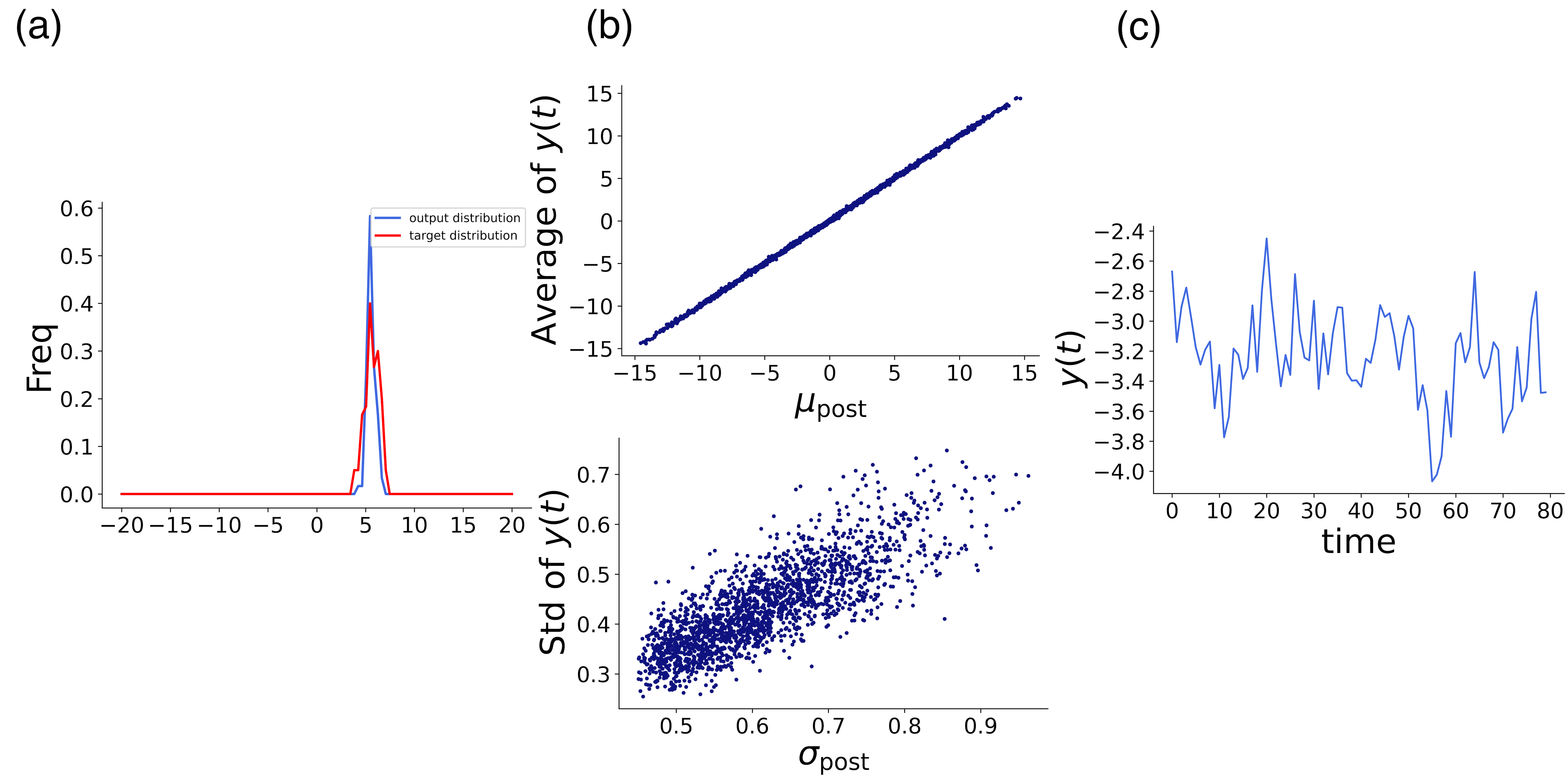
As a result of training, the distribution of the network output for both FFNN and RNN approached the posterior distribution [Fig. 2(a)]. The mean and variance of were similar to those obtained from Eqs. (1, 2) (Fig. 2(b)). In addition, Fig. 2(c) shows the output timeseries is stochastically generated, not periodically. These results suggest that the ANNs successfully learned to perform sampling-based inference from the posterior distribution in the cue-combination task. We also confirmed that these ANNs could learn to perform sampling-based probabilistic inference in another cognitive task (see Appendix B).
Here, accuracy computed by comparing the mean and the variance of the outputs of Eqs. (1) and (2) in terms of mean squared error (MSE) were higher in the RNN than in the FFNN, especially in the variance, suggesting that the RNN performed sampling-based inference more efficiently (Fig.3). We also found that the FFNN and RNN could perform efficient information processing from the perspective of information theory and confirm that RNN can more efficiently process input information than FFNN(See Appendix C).
In this section, the analyses of the mechanism of sampling behavior in the FFNN and RNN are described.
3.1 Sampling mechanism in the FFNN
To accurately perform sampling from the posterior distribution, the NN needs to manipulate the output variability using stochastic perturbations of the input signals. Here, as shown in Eqs. (3, 4), the input signals have Poisson-like variability, and their mean and variance increase linearly with the gain . However, as the gain corresponds to the input signals’ reliability, the variance of the posterior distribution decreases as increases. It means that the network should have an internal mechanism to reverse the magnitude of variances of the input and output. Here, we clarify the mechanism that transforms the input signal variance to output variance in FFNN. First, there are two possible candidates for where the variance transformation occurs: the input layer to the hidden layer and the hidden layer to the output layer. As the magnitude of the fluctuation of the hidden layer activity strictly correlates to the standard deviation of the posterior distribution [Fig. 4(a)], this variance transformation is supposed to occur when the signal is transformed from the input layer to the hidden layer. In the following, we reveal the mechanism of this variance transformation by focusing on the transformation of signals from the input layer to the hidden layer.
Focusing on a single neuron in the hidden layer, we investigated how differences in the gain of the input signal affect the neuronal activity in that hidden layer. For simplicity, we set . Comparing the results for and , we found that the distribution of the amount of activity obtained by the linear transformation from the input layer widened and shifted to the left as increased [Fig. 4(b)]. Indeed, this tendency is supported by the statistics of the input matrix and the bias ; the mean values of and , respectively, satisfy and . Here, considering nonlinearity, the variance of the hidden layer is affected only by hidden neurons with activities greater than , from which a negative correlation between and can be derived.
Assuming that the above mechanism is in the FFNN, the number of hidden neurons with values greater than decreases, i.e., the hidden layer gets sparser. In fact, an analysis shows that a sparsity-based coding is present [Fig. 4(c)]. This sparsity-based coding is similar to the coding in MAP estimation by FFNN (Orhan and Ma, 2017).
3.2 Sampling mechanism in the RNN
Now, we discuss the sampling mechanism in the RNN. In the RNN, the relationship between the fluctuation of the hidden layer firing rate and the standard deviation of the posterior distribution is nonmonotonic, which differs from the result in the FFNN [(Fig.5(a)]. Here, the variation of and the standard deviation are negatively correlated in the region where is small, whereas they are positively correlated in the region where is large.
First, we found that when the input signals were stationary, the dynamics of the hidden layer converged to certain fixed points. Each of these fixed points corresponds to a pair of mean and standard deviation of the posterior distribution . Hence, we can decompose the dynamics of the hidden layer to fixed-point neural states and the fluctuation around them. Assuming that the fluctuation is sufficiently small, we can linearize the dynamics around a fixed point (Sussillo and Barak, 2013), and it yields
| (14) |
where
and
The term represents a Jacobian matrix near the corresponding fixed point , which determines the characteristics of the landscape of neural dynamics (Maheswaranathan et al., 2019). Meanwhile, the term corresponds to the fluctuation of the input signal. It is conceivable that the mechanism underlying sampling-based inference in the RNN is a combination of effects from these two terms.
Hence, we investigated the relationships among the largest eigenvalues of the Jacobian matrix near each fixed point, the fluctuation of the hidden layer activities, and the standard deviation [Fig. 5(b, c)].
Comparing this result with the relationship between the fluctuation of the hidden layer firing rate and standard deviation [Fig. 5(a)], in the region where is small, the trend is similar to the change in [Fig. 5(b)], whereas, in the region where is large, the trend is similar to the change in the largest eigenvalues of the Jacobian matrix [Fig. 5(c)].
In the following, we discuss the mechanism of controlling the variance of the output in each of the two areas: small- and large-variance areas.
3.2.1 Small-variance area
When the standard deviation of the posterior distribution is small, different from the FFNN case, the posterior deviation and the fluctuation of in RNN positively correlate. It may naively seem that the variance is incontrollable. However, as the output signal is determined as an inner product of the hidden activity and readout vector , the direction of the fluctuation of also needs to be considered, and it can explain the mechanism. Let us consider a matrix given by temporally ordered hidden activities and perform eigenvalue decomposition of a covariance matrix as follows:
| (15) |
where . Each eigenvector corresponds to a principal component (PC) of (Jolliffe and Cadima, 2016).
We elucidate how each PC affects the variance of the output . As shown in Fig. 6(a), the first and second components are nearly orthogonal to , which implies they slightly affect the variance of the output. Meanwhile, the third to fifth PCs significantly affect the output variance via solid correlation from the sum of inner products with to (fig. 6(b)). Further, quantifying the fluctuation directions of the internal dynamics as angles between and eigenvectors of these (from the third to fifth) PCs shows that these directions negatively correlate with the posterior variance in the area where is small. Although the effect on the output is determined by the magnitude of the fluctuations of and their directions, the results show that when is relatively small, the output variance is controlled by the directions of the fluctuations [Fig. 6(c)].
3.2.2 Large-variance area
In the area with large posterior variance, the correlation between the variance and angles of PCs and the readout vector is weak, which implies that, in the large-variance area, the output variance is simply controlled by the magnitude of the fluctuation of the internal dynamics . In fact, Fig. 5(a) shows a positive correlation between and fluctuation of in the large-variance area. However, the input variance does not correlate with , which means that the landscape of the internal dynamics controls the output fluctuation. The largest eigenvalue of the Jacobian matrix represents stability against noise around fixed point ; under a constant amplitude of noise, the larger this value is, the larger the fluctuation of the internal dynamics. Fig. 5 shows the correlation between the largest eigenvalues and posterior variance , suggesting that they control the fluctuations of .
Summarizing the above results, two attributes contribute to the control of sampling in RNNs (Fig.7):
-
•
Small-variance area: The magnitude of the fluctuations of the internal dynamics is predominantly determined by the fluctuations of the input signal, and the variance of the output signal is controlled by the “direction” of the fluctuations of the internal dynamics.
-
•
Large-variance area: The magnitude of the fluctuations of the internal dynamics is predominantly determined by the landscape of dynamics around the fixed point, and the variance of the output signal is controlled by the “magnitude” of the fluctuations of the internal dynamics.
RNNs can reasonably perform more accurate inferences than FFNNs in which only input fluctuation contributes to controlling sampling.
Since RNNs have a larger number of parameters than FFNNs when the numbers of neurons are fixed, we also tested their accuracy under a fixed number of parameters. The results still indicated the superiority of the RNN, implying that the superiority is not simply caused by the richness of parameters (see Appendix D).
3.3 Sampling as inductive bias
This subsection shows the results of a comparison of sampling-based probabilistic inference with point estimation. Here, we used MAP estimation as an example of point estimation and trained NNs to output . Notably, Eq. (1) claims MAP estimation still requires NNs to consider standard deviations . The loss function for MAP estimation is defined as mean squared error(MSE):
| (16) |
This setting has already been studied and shown to be possible to learn for ANNs (Orhan and Ma, 2017). In this study, we also confirmed the performance of NNs on the point estimation task (fig. 8(a)).
To compare sampling-based and MAP probabilistic inferences, we evaluated accuracies in terms of MSE between time-averaged outputs and mean value of the posterior distribution given various inputs as follows:
| (17) |
Remarkably, the results showed the RNN is more accurate in the sampling-based task than in the MAP task (fig.8(c)). In other words, the sampling-based probabilistic inference on the posterior distribution works as an inductive bias in the estimation of the posterior mean. Notably, this difference in accuracy between MAP estimation and sampling is subtle in the FFNN [Fig. 8(b)].
In the RNN trained to perform point estimation, each pair of the mean and standard deviations corresponds to a fixed point similar to the sampling-based task. Since it is implied that the geometry of these fixed points affects the accuracy of the output (Cohen et al., 2020), we analyzed it.
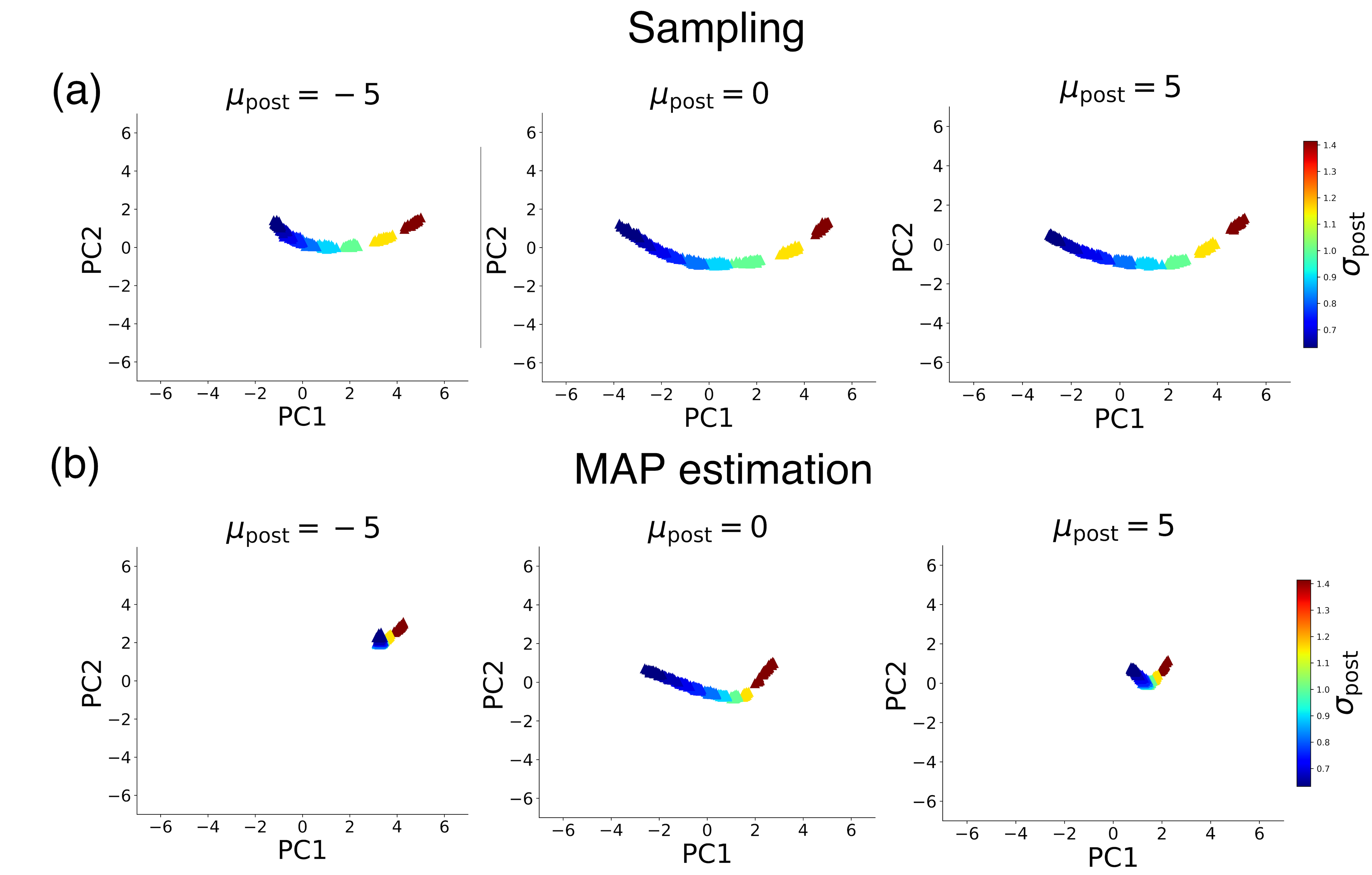
Fig. 9 shows that takes different positions when varies, even if is constant. By contrast, the output is required to be fixed when is fixed, regardless of the changes in . To fulfill this requirement, the NNs need readout vector to be aligned orthogonal to the direction in which fixed points move depending on . Since this condition should be satisfied for every , changes in are expected to be small when is fixed and is variable.
Assuming that is sufficiently low-dimensional, the varying direction of is characterized by PCs. Hence, for a detailed characterization, we projected a set (manifold) of fixed points given onto the first and second PCs computed under . If the direction along which the fixed points move for different does not change when varies, the projection of the manifold must also look invariant. As shown in Fig.9, the NN trained on the sampling-based task satisfies these conditions while the geometry of the fixed-point manifold in the point estimation NN is apparently variant to .
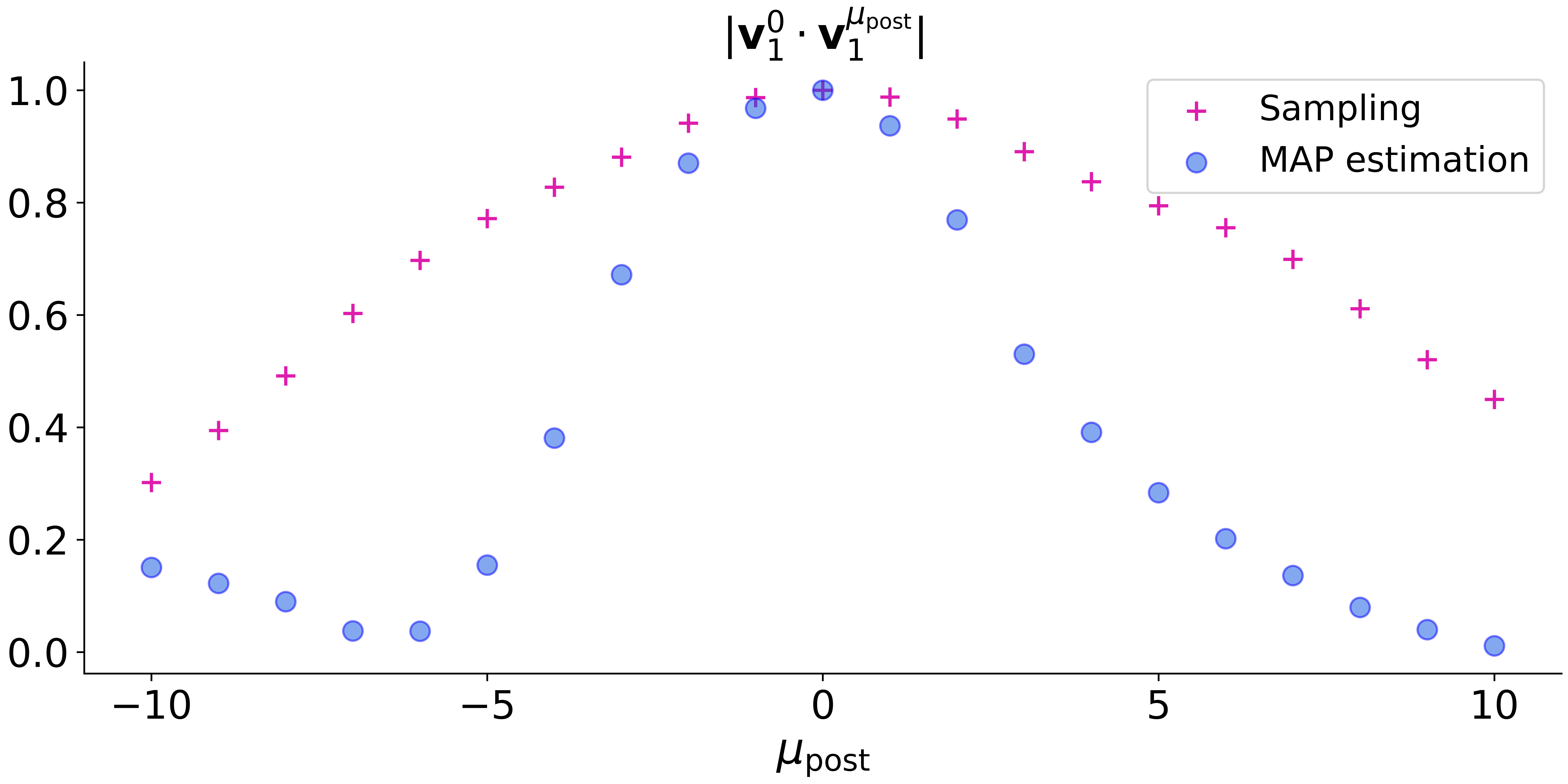
Quantitatively, these geometric characteristics can be investigated in terms of absolute inner product of fixed point given a posterior mean and as . takes values within the range ; the larger this value is, the more parallel manifolds for different posterior means are aligned. This quantity takes larger values in the NN trained on sampling-based inference (fig. 10), which means that the manifolds are more nearly parallel to each other than in the NN for point estimation. This characteristic implies a mechanism wherein the NN can output proper values depending only on , independent of , by choosing the readout vector appropriately, and this mechanism underlies the superiority of the RNN trained on sampling to the one trained on MAP estimation.
These geometric characteristics in sampling might be due to the learning strategy that explicitly includes effects of in the output . In summary, this is an example of inductive bias (Baxter, 2000; Whigham, 1995; Helmbold and Long, 2015; Haussler, 1988) in which a constraint leads to better accuracy in estimating .
4 Discussion
In this study, we trained two types of ANNs, the FFNN and the RNN, on the cue-combination task to investigate their dynamical mechanisms and characteristics of performing sampling-based probabilistic inferences. To achieve this, we made input signals encoding external cues by PPC and trained the ANNs to generate the output as a sampling of posterior probability distribution using the gradient descent scheme.
First, the results showed that training was successful for both ANNs. Hence, sampling-based probabilistic inferences are possible using the ANNs. However, the mechanisms underlying the sampling in FFNN and RNN differ: the FFNN adjusts amplitudes of the fluctuation of the input signals appropriately when they are feed-forwarded into the hidden layer to realize a sampling from the posterior distribution; whereas, in the RNN, dynamics in the hidden layer, which can be decomposed into fixed points and perturbations around them, play a crucial role in the sampling. Moreover, it was revealed that the RNN employs two different mechanisms depending on the posterior variance. When the posterior variance was small, the angle of the fluctuation of the internal state was considered, whereas the landscape of the system near fixed points was manipulated when the posterior variance was large. It is also suggested that this difference in the sampling mechanisms leads to the superiority of the RNN in terms of accuracy.
Further, we trained the FFNN and RNN on a similar cue-combination task but in a MAP estimation setting, not sampling-based, to compare the sampling-based probabilistic inference with point estimation. The results showed that, in the RNN, the accuracy of estimating mean values of the posterior distribution via sampling was higher than that via point estimation, which could be explained by differences in geometric characteristics, and that might be an example of the roles of the sampling as an inductive bias. The changes in the fixed-point manifolds constructed by varying posterior variance for different were more parallel to each other in the NN trained to perform the sampling than in that trained for point estimation, leading to ease for the readout vector alignment to be invariant to changes in the posterior variance , which accurizes the NN (Susman et al., 2021). This characteristic can be thought to be obtained under constraints in which the NN needs to constantly behave for different .
In this study, we first clarified the utility of sampling in information processes. In addition, it is suggested that the sampling can contribute to good performance in estimating important statistics, such as the MAP inference, not only in the estimation of ambiguities of information. If the sampling mechanisms in this study are equipped in the brain, a comparison of the accuracy between point estimation and sampling-based inference would also show a similar result.
We also highlighted differences between FFNNs and RNNs. In a previous study (Orhan and Ma, 2017), FFNN was mainly trained on the point estimation setting, and differences with RNNs were not discussed. However, considering the sampling, there were clear differences between them in terms of accuracy and mechanism. These results can provide arguments on the significance of recurrent connections among neurons in the brain from another perspective. Particularly, this study suggested important results to investigate what roles dynamical characteristics in the information process play (Orhan and Ma, 2019).
As we would like to investigate the relationships between the sampling mechanism and PPC for the first step, we did not add the internal noise in neural dynamics. However, internal noise is universally present in the brain, and it probably contributes to implementing probabilistic inference. Indeed, previous studies have investigated the sampling inference of RNN driven by the internal noise(Echeveste et al., 2020; Aitchison and Lengyel, 2016). Hence, how internal noise and noise due to PPC each affect sampling needs to be investigated in more detail. In addition, for simplicity, we adopted a model that assumes that PPC is uncorrelated between input neurons. However, since a large body of work shows that neurons can be correlated (Averbeck et al., 2006; Moreno-Bote et al., 2014), it is important to examine PPC that correlates among input neurons.
The model we used for our research is an idealized model, and there are differences in the way the brain actually works. For instance, The models employed in this study were trained using the back-propagation algorithm (Werbos, 1990), and the loss function was KLD, which is an artificial setting. Although it is still a matter of debate as to what kind of training algorithm is equipped in the actual brain (Lillicrap et al., 2020; Whittington and Bogacz, 2019), many reports are claiming that the behaviors of ANNs trained using the back-propagation algorithm are often similar to activities in the brain (Richards et al., 2019; Yang and Wang, 2020; Mante et al., 2013), even though it is said to be physiologically implausible (Bengio et al., 2015; Lillicrap et al., 2016). Therefore, we expect that the results from this study agree with the dynamical features of the brain known from previous physiological studies or those that will be revealed in future studies.
Acknowledgments
The authors would like to express their gratitude to Kunihiko Kaneko and Tetsuhiro S. Hatakeyama for their comments and discussions.
Appendix A: Input signals
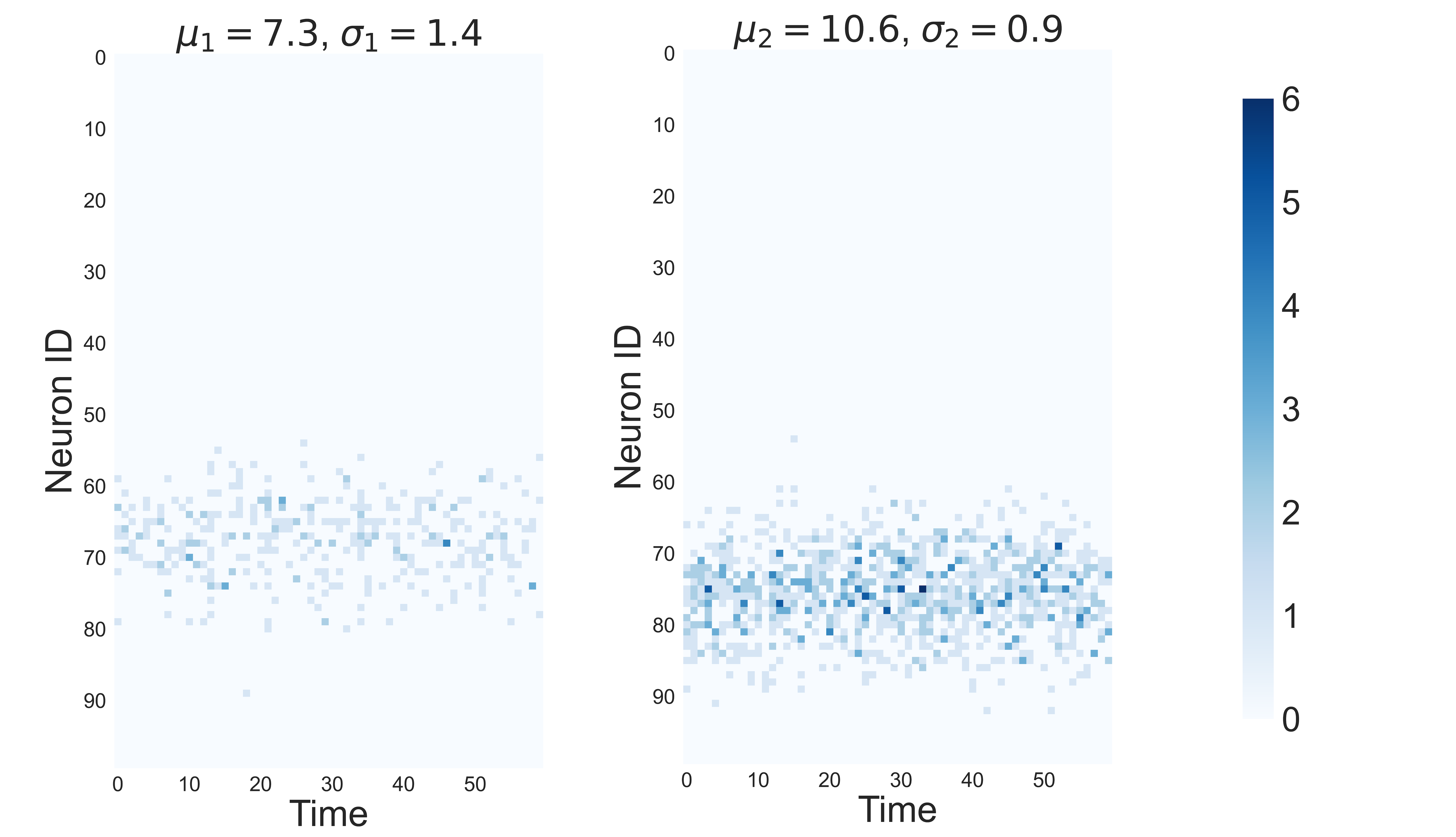
The input signal is generated stochastically according to Eqs. (3), (4), as shown in Fig.11. The two signals and shown in the figure encode the input information with different mean and standard deviation , respectively. The signal of has a smaller and greater certainty of information. fires more strongly than because is larger than .
Appendix B: Coordinate Transformation Task
To verify that sampling-based inference is possible for other tasks, we trained the coordinate transformation task introduced in (Beck et al., 2011). This task considers the same setting as the cue-combination task, where signals following two gaussian distributions are input, but the posterior distribution to be inferred is given by a gaussian distribution with the following mean and variance:
| (18) | ||||
| (19) |
When this task was trained, the distribution of the output became closer to the posterior distribution through learning(Fig.14(a)), and the mean and the standard deviation of the output had values close to the mean and the standard deviation of the posterior distribution(Fig.14(b)). It was also confirmed that the output behaved stochastically, as shown in Fig.14(c). From these results, it was found that NNs could learn sampling-based inference in the coordinate transformation task setting as well as the cue-combination task.
Appendix C: Information efficiency in the NNs
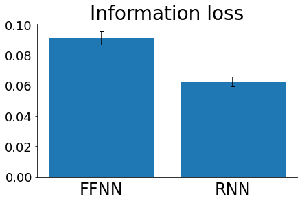
To see how efficient the information processing performed by the networks is, we computed information losses of the FFNN and RNN. Information loss is computed as KLD from the optimal posterior distribution to the histogram of outputs of a network, normalized by mutual information between input cue and label data (Qamar et al., 2013):
The results show that in both of the FFNN and the RNN, the computed information losses are low, which suggest these networks can perform efficient information processing. By comparing the information loss between the two networks, one can see that it is lower in the RNN. This comparison can also be a support for the claim that the RNN performs more efficient sampling-based probabilistic inference.
Appendix D: Effect of the size of NNs
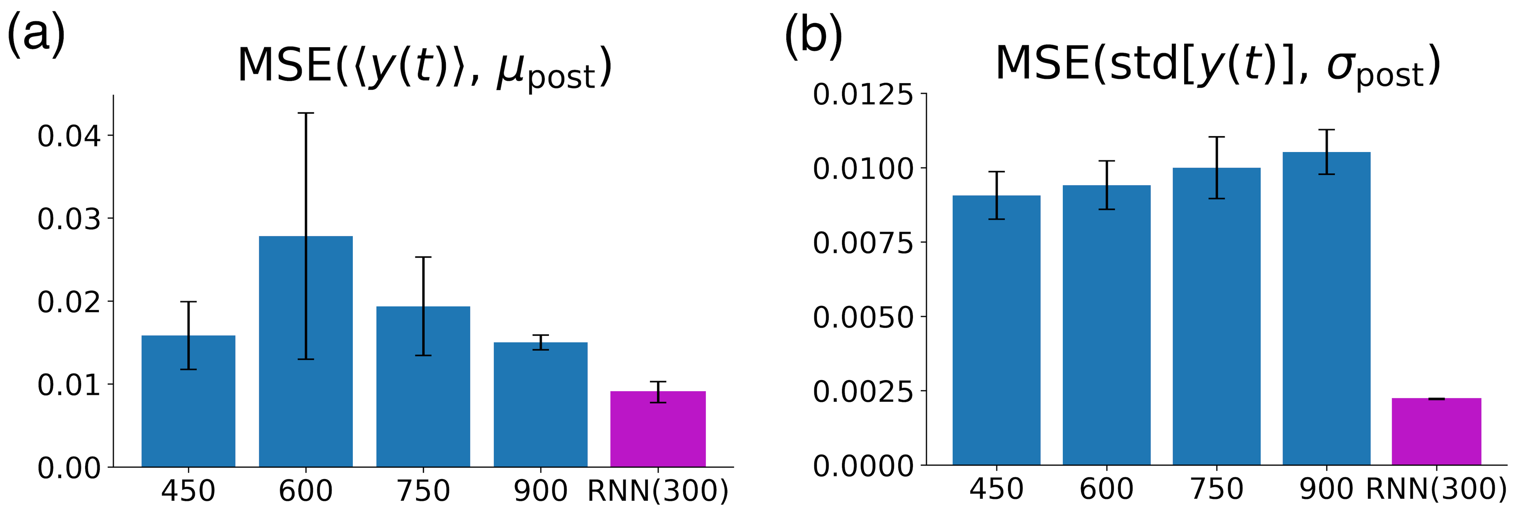
To confirm that the difference in accuracy between FFNN and RNN is fundamental one, we trained the cue-combination task in FFNN with different size of NNs and compared the accuracy. The FFNN with 750 internal neurons and the RNN with 300 internal neurons have similar number of parameters.
Although the accuracies are different depending on the size, the difference between FFNN and RNN, especially the accuracy on standard deviation, is remarkable(Fig.12). The result shows that there is a fundamental difference in accuracy between FFNN and RNN as discussed in the main part.
References
- Aitchison and Lengyel (2016) Aitchison, L. and Lengyel, M. (2016). The hamiltonian brain: Efficient probabilistic inference with excitatory-inhibitory neural circuit dynamics. PLOS Computational Biology, 12(12):1–24.
- Angelaki et al. (2009) Angelaki, D. E., Gu, Y., and DeAngelis, G. C. (2009). Multisensory integration: psychophysics, neurophysiology, and computation. Current Opinion in Neurobiology, 19(4):452–458. Sensory systems.
- Averbeck et al. (2006) Averbeck, B. B., Latham, P. E., and Pouget, A. (2006). Neural correlations, population coding and computation. Nature Reviews Neuroscience, 7(5):358–366.
- Bányai et al. (2019) Bányai, M., Lazar, A., Klein, L., Klon-Lipok, J., Stippinger, M., Singer, W., and Orbán, G. (2019). Stimulus complexity shapes response correlations in primary visual cortex. PNAS, 116(7):2723–2732.
- Barak (2017) Barak, O. (2017). Recurrent neural networks as versatile tools of neuroscience research. Current Opinion in Neurobiology, 46:1–6. Computational Neuroscience.
- Baxter (2000) Baxter, J. (2000). A model of inductive bias learning. J. Artif. Int. Res., 12(1):149–198.
- Beck et al. (2011) Beck, J. M., Latham, P. E., and Pouget, A. (2011). Marginalization in neural circuits with divisive normalization. Journal of Neuroscience, 31(43):15310–15319.
- Beck et al. (2008) Beck, J. M., Ma, W. J., Kiani, R., Hanks, T., Churchland, A. K., Roitman, J., Shadlen, M. N., Latham, P. E., and Pouget, A. (2008). Probabilistic population codes for bayesian decision making. Neuron, 60(6):1142–1152.
- Bengio et al. (2015) Bengio, Y., Lee, D., Bornschein, J., and Lin, Z. (2015). Towards biologically plausible deep learning. ArXiv, abs/1502.04156.
- Chung et al. (2018) Chung, S., Lee, D. D., and Sompolinsky, H. (2018). Classification and geometry of general perceptual manifolds. Phys. Rev. X, 8:031003.
- Cohen et al. (2020) Cohen, U., Chung, S., Lee, D. D., and Sompolinsky, H. (2020). Separability and geometry of object manifolds in deep neural networks. Nature Communications, 11(1):746.
- Doya et al. (2007) Doya, K., Ishii, S., Pouget, A., and Rao, R. P. N. (2007). Bayesian Brain: Probabilistic Approaches to Neural Coding. MIT Press.
- Echeveste et al. (2020) Echeveste, R., Aitchison, L., Hennequin, G., and Lengyel, M. (2020). Cortical-like dynamics in recurrent circuits optimized for sampling-based probabilistic inference. Nature Neuroscience, 23(9):1138–1149.
- Ernst and Banks (2002) Ernst, M. O. and Banks, M. S. (2002). Humans integrate visual and haptic information in a statistically optimal fashion. Nature, 415(6870):429–433.
- Haefner et al. (2016) Haefner, R. M., Berkes, P., and Fiser, J. (2016). Perceptual decision-making as probabilistic inference by neural sampling. Neuron, 90(3):649–660.
- Haussler (1988) Haussler, D. (1988). Quantifying inductive bias: Ai learning algorithms and valiant’s learning framework. Artificial Intelligence, 36(2):177–221.
- Helmbold and Long (2015) Helmbold, D. P. and Long, P. M. (2015). On the inductive bias of dropout. Journal of Machine Learning Research, 16(105):3403–3454.
- Jolliffe and Cadima (2016) Jolliffe, I. T. and Cadima, J. (2016). Principal component analysis: a review and recent developments. Philosophical Transactions of the Royal Society A: Mathematical, Physical and Engineering Sciences, 374(2065):20150202.
- Kingma and Ba (2014) Kingma, D. P. and Ba, J. (2014). Adam: A method for stochastic optimization.
- Knill and Pouget (2004) Knill, D. C. and Pouget, A. (2004). The bayesian brain: the role of uncertainty in neural coding and computation. Trends in Neurosciences, 27(12):712–719.
- LeCun et al. (2015) LeCun, Y., Bengio, Y., and Hinton, G. (2015). Deep learning. Nature, 521:436–444.
- Lillicrap et al. (2016) Lillicrap, T. P., Cownden, D., Tweed, D. B., and Akerman, C. J. (2016). Random synaptic feedback weights support error backpropagation for deep learning. Nature Communications, 7(1):13276.
- Lillicrap et al. (2020) Lillicrap, T. P., Santoro, A., Marris, L., Akerman, C. J., and Hinton, G. (2020). Backpropagation and the brain. Nature Reviews Neuroscience, 21(6):335–346.
- Ma et al. (2006) Ma, W. J., Beck, J. M., Latham, P. E., and Pouget, A. (2006). Bayesian inference with probabilistic population codes. Nature Neuroscience, 9(11):1432–1438.
- Ma et al. (2008) Ma, W. J., Beck, J. M., and Pouget, A. (2008). Spiking networks for bayesian inference and choice. Current Opinion in Neurobiology, 18(2):217–222. Cognitive neuroscience.
- Maheswaranathan et al. (2019) Maheswaranathan, N., Williams, A., Golub, M., Ganguli, S., and Sussillo, D. (2019). Universality and individuality in neural dynamics across large populations of recurrent networks. In Wallach, H., Larochelle, H., Beygelzimer, A., d'Alché-Buc, F., Fox, E., and Garnett, R., editors, Advances in Neural Information Processing Systems, volume 32. Curran Associates, Inc.
- Mante et al. (2013) Mante, V., Sussillo, D., Shenoy, K. V., and Newsome, W. T. (2013). Context-dependent computation by recurrent dynamics in prefrontal cortex. Nature, 503(7474):78–84.
- Merfeld et al. (1999) Merfeld, D. M., Zupan, L., and Peterka, R. J. (1999). Humans use internal models to estimate gravity and linear acceleration. Nature, 398(6728):615–618.
- Moreno-Bote et al. (2014) Moreno-Bote, R., Beck, J., Kanitscheider, I., Pitkow, X., Latham, P., and Pouget, A. (2014). Information-limiting correlations. Nature Neuroscience, 17(10):1410–1417.
- Moreno-Bote et al. (2011) Moreno-Bote, R., Knill, D. C., and Pouget, A. (2011). Bayesian sampling in visual perception. Proceedings of the National Academy of Sciences, 108(30):12491–12496.
- Nair and Hinton (2010) Nair, V. and Hinton, G. E. (2010). Rectified linear units improve restricted boltzmann machines. In Fürnkranz, J. and Joachims, T., editors, ICML, pages 807–814. Omnipress.
- Orbán et al. (2016) Orbán, G., Berkes, P., Fiser, J., and Lengyel, M. (2016). Neural variability and sampling-based probabilistic representations in the visual cortex. Neuron, 92(2):530–543.
- Orhan and Ma (2017) Orhan, A. E. and Ma, W. J. (2017). Efficient probabilistic inference in generic neural networks trained with non-probabilistic feedback. Nature Communications, 8(1):138.
- Orhan and Ma (2019) Orhan, A. E. and Ma, W. J. (2019). A diverse range of factors affect the nature of neural representations underlying short-term memory. Nature Neuroscience, 22(2):275–283.
- Qamar et al. (2013) Qamar, A. T., Cotton, R. J., George, R. G., Beck, J. M., Prezhdo, E., Laudano, A., Tolias, A. S., and Ma, W. J. (2013). Trial-to-trial, uncertainty-based adjustment of decision boundaries in visual categorization. Proceedings of the National Academy of Sciences, 110(50):20332–20337.
- Richards et al. (2019) Richards, B. A., Lillicrap, T. P., Beaudoin, P., Bengio, Y., Bogacz, R., Christensen, A., Clopath, C., Costa, R. P., de Berker, A., Ganguli, S., Gillon, C. J., Hafner, D., Kepecs, A., Kriegeskorte, N., Latham, P., Lindsay, G. W., Miller, K. D., Naud, R., Pack, C. C., Poirazi, P., Roelfsema, P., Sacramento, J., Saxe, A., Scellier, B., Schapiro, A. C., Senn, W., Wayne, G., Yamins, D., Zenke, F., Zylberberg, J., Therien, D., and Kording, K. P. (2019). A deep learning framework for neuroscience. Nature Neuroscience, 22(11):1761–1770.
- Susman et al. (2021) Susman, L., Mastrogiuseppe, F., Brenner, N., and Barak, O. (2021). Quality of internal representation shapes learning performance in feedback neural networks. Phys. Rev. Research, 3:013176.
- Sussillo and Barak (2013) Sussillo, D. and Barak, O. (2013). Opening the Black Box: Low-Dimensional Dynamics in High-Dimensional Recurrent Neural Networks. Neural Computation, 25(3):626–649.
- Svozil et al. (1997) Svozil, D., Kvasnicka, V., and Pospichal, J. (1997). Introduction to multi-layer feed-forward neural networks. Chemometrics and Intelligent Laboratory Systems, 39(1):43–62.
- Tanabe (2013) Tanabe, S. (2013). Population codes in the visual cortex. Neuroscience research, 76(3):101–105.
- Tolhurst et al. (1983) Tolhurst, D., Movshon, J., and Dean, A. (1983). The statistical reliability of signals in single neurons in cat and monkey visual cortex. Vision Research, 23(8):775–785.
- van Beers et al. (1999) van Beers, R. J., Sittig, A. C., and Gon, J. J. D. v. d. (1999). Integration of proprioceptive and visual position-information: An experimentally supported model. Journal of Neurophysiology, 81(3):1355–1364. PMID: 10085361.
- Vyas et al. (2020) Vyas, S., Golub, M. D., Sussillo, D., and Shenoy, K. V. (2020). Computation through neural population dynamics. Annu. Rev. Neurosci., 43:249–275.
- Walker et al. (2020) Walker, E. Y., Cotton, R. J., Ma, W. J., and Tolias, A. S. (2020). A neural basis of probabilistic computation in visual cortex. Nature Neuroscience, 23(1):122–129.
- Werbos (1990) Werbos, P. J. (1990). Backpropagation through time: what it does and how to do it. Proceedings of the IEEE, 78(10):1550–1560.
- Whigham (1995) Whigham, P. (1995). Inductive bias and genetic programming. IET Conference Proceedings, pages 461–466(5).
- Whittington and Bogacz (2019) Whittington, J. C. and Bogacz, R. (2019). Theories of error back-propagation in the brain. Trends in Cognitive Sciences, 23(3):235–250.
- Yang and Wang (2020) Yang, G. R. and Wang, X.-J. (2020). Artificial neural networks for neuroscientists: A primer. Neuron, 107(6):1048–1070.