Abstract

Bayesian neural networks that incorporate data augmentation implicitly use a “randomly perturbed log-likelihood [which] does not have a clean interpretation as a valid likelihood function” (Izmailov et al. 2021). Here, we provide several approaches to developing principled Bayesian neural networks incorporating data augmentation. We introduce a “finite orbit” setting which allows likelihoods to be computed exactly, and give tight multi-sample bounds in the more usual “full orbit” setting. These models cast light on the origin of the cold posterior effect. In particular, we find that the cold posterior effect persists even in these principled models incorporating data augmentation. This suggests that the cold posterior effect cannot be dismissed as an artifact of data augmentation using incorrect likelihoods.

 

Data augmentation in Bayesian neural networks
and the cold posterior effect

 

Seth Nabarro*                        Stoil Ganev*                        Adrià Garriga-Alonso

Department of Computing Imperial College London London, SW7 2BX, UK seth.nabarro09@imperial.ac.uk                        Department of Computer Science University of Bristol Bristol, BS8 1UB, UK                        Department of Engineering University of Cambridge Cambridge, CB2 1PZ, UK ag919@cam.ac.uk

Vincent Fortuin                        Mark van der Wilk†                        Laurence Aitchison† Department of Computer Science, ETH Zürich, Zürich, Switzerland                        Department of Computing Imperial College London London, SW7 2BX, UK m.vdwilk@imperial.ac.uk                        Department of Computer Science University of Bristol Bristol, BS8 1UB, UK laurence.aitchison@gmail.com

1 INTRODUCTION

The cold posterior effect (CPE; Wenzel et al.,, 2020) is the surprising observation that performance in neural networks is not optimal when we use the usual Bayesian posterior (Kolmogorov,, 1950; Savage,, 1954; Jaynes,, 2003),

$$\operatorname{P}\left(\mathbf{w}\middle|\mathbf{y},\mathbf{X}\right)\propto\operatorname{P}\left(\mathbf{w}\right)\operatorname{P}\left(\mathbf{y}\middle|\mathbf{w},\mathbf{X}\right)$$ (1)

where $\mathbf{w}$ are the neural network weights, $\mathbf{X}$ is all inputs (typically images), and $\mathbf{y}$ is all outputs (typically class labels). Instead, we get better performance when using a “cold” posterior, i.e. the posterior taken to the power of $1/T$ where $T<1$,

$$\operatorname{Q}\left(\mathbf{w}\right) \propto\left(\operatorname{P}\left(\mathbf{w}\right)\operatorname{P}\left(\mathbf{y}\middle|\mathbf{w},\mathbf{x}\right)\right)^{1/T}.$$ (2)

The origin of the CPE is by now highly contentious, with three leading potential explanations (Noci et al.,, 2021). The first hypothesis is that the process of data curation for popular datasets such as CIFAR-10 and ImageNet (Krizhevsky et al.,, 2009; Deng et al.,, 2009) involves multiple annotators agreeing upon the label for each image. In that case, there are in effect multiple labels for each image, which inflates the likelihood (but not the prior) term in the cold posterior (Adlam et al.,, 2020; Aitchison,, 2020). Second, the prior is always misspecified, and prior misspecification is known to induce cold posterior-like effects in specific (non-neural network) models (Grünwald,, 2012; Grünwald et al.,, 2017), which might give an explanation for the CPE in neural networks (Wenzel et al.,, 2020; Fortuin et al., 2021b, ). However, Fortuin et al., 2021b showed that better priors do not always reduce the size of the CPE, but can actually increase it. In particular, they found that incorporating spatial correlations in convolutional filters improved the performance of a ResNet trained on CIFAR-10, but also increased the magnitude of the CPE. Third, there is the possibility that the CPE is an artifact of data augmentation (DA; Wenzel et al.,, 2020; Izmailov et al.,, 2021), as DA gives a “randomly perturbed log-likelihood [which] does not have a clean interpretation as a valid likelihood function” (Izmailov et al.,, 2021). This is supported by observations in which the CPE only exists with DA, and disappears without DA (Wenzel et al.,, 2020; Fortuin et al., 2021b, ; Izmailov et al.,, 2021). Of course it is quite possible that practical CPEs arise from a complex combination of these causes (Aitchison,, 2020; Noci et al.,, 2021).

In spite of this controversy, recent work on the CPE agrees that it is important to investigate integrating DA with Bayesian neural networks (BNNs), and to examine the interaction with the CPE. From Noci et al., (2021): “It remains an interesting open problem how to properly account for data augmentation in a Bayesian sense.” And from Izmailov et al., (2021): “Data augmentation cannot be naively incorporated in the Bayesian neural network model.” And “We leave incorporating data augmentation … as an exciting direction of future work.”

Perhaps the most common understanding of the interaction between the CPE and DA in BNNs is that DA increases the effective dataset size. From Izmailov et al., (2021): “intuitively, data augmentation increases the amount of data observed by the model, and should lead to higher posterior contraction”. From Osawa et al., (2019): “DA increases the effective sample size”. From, Noci et al., (2021): “while data augmentation may increase the amount of data seen by the model, that increase is certainly not equal to the number of times each data point is augmented (after all, augmented data is not independent from the original data).”

In this paper, we first give a formal argument that the notion that DA increases the effective dataset size is flawed. Second, we consider issues with the current training objectives for Bayesian generative models which incorporate DA (van der Wilk et al.,, 2018; Wenzel et al.,, 2020). In particular, Wenzel et al., (2020) proposed a single-sample training objective that Izmailov et al., (2021) regarded as a “randomly perturbed log-likelihood [which] does not have a clean interpretation as a valid likelihood function”, and van der Wilk et al., (2018) proposed a training objective that only works for quadratic log-likelihoods (i.e. Gaussians or Pólya-Gamma approximations). We show that multi-sample estimators which average network logits or probabilities form lower bounds on the intractable log-likelihoods of principled Bayesian models. These bounds are tighter than the single-sample estimators used previously in the Bayesian setting (e.g. Wenzel et al.,, 2020) and can be applied to a broad class of likelihood functions (unlike van der Wilk et al.,, 2018). Third, we introduce a “finite orbit” setting with a small number of admissible augmentations which allows us to compute exact log-likelihoods. Fourth, we give the natural generalizations beyond classification to arbitrary outputs (Appendix D). Fifth, we show that the CPE persists even when using these principled DA likelihoods (it certainly is the case that the CPE could have been an artifact of loose bounds arising from previous single-sample estimators). Finally, we consider the consequences for explanations of the CPE. In particular, we can no longer conclude that the CPE is an artifact resulting from DA giving an invalid likelihood function (Izmailov et al.,, 2021), as we have a principled Bayesian model incorporating DA. In the finite orbit setting, we can compute the exact likelihood, while in the usual setting there is in principle a deterministic likelihood with a clean interpretation as a valid likelihood function, but as this is difficult to evaluate in practice we use a tight multi-sample lower bound.

Note that in the remainder of the paper, we will follow Izmailov et al., (2021) in regarding models with loose, single-sample bounds as “unprincipled” (from Izmailov et al., (2021), the “randomly perturbed log-likelihood does not have a clean interpretation as a valid likelihood function”). In contrast, we term models using our exact log-likelihoods or our tight multi-sample bounds as being “principled”.

2 BACKGROUND

2.1 Data augmentation

In supervised learning, we are interested in learning some unknown functional relationship from example input-output pairs $(\mathbf{x}_{i},y_{i}),i=1,\ldots,N$. Usually, we have information about some form of invariance, i.e. the knowledge that the function does not change its output for certain transformations of the input. These might occasionally be true invariances, such as the identity of a molecule being invariant to rotations. But in most settings, these are so-called “soft” invariances or “insensitivities” (van der Wilk et al.,, 2018). For instance the class label for an image should not change due to small translations/crops of that image (but might change if we radically alter the image). The most basic form of data augmentation takes advantage of this information by transforming, or augmenting, the inputs and copying the output value, to create additional input-output pairs which are then included in training. Often, the amount of additional “augmented data” can be unbounded, for example when allowable transformations are specified in a continuous range, e.g. rotations. This simple procedure has been very successful in improving performance in a wide variety of machine learning methods (Loosli et al.,, 2007; Krizhevsky et al.,, 2012; Bishop,, 2006), and recent work has analysed the effect of data augmentation on invariances in the learned functions (Dao et al.,, 2019; Chen et al.,, 2020; Lyle et al.,, 2020).

2.2 Bayesian inference

Bayesian inference allows us to infer a distribution over neural network weights, which incorporates uncertainty induced by having finite data. Bayes prescribes a strict procedure for updating beliefs about unknown quantities in light of observed data. The model is specified by a prior on the weights $\operatorname{P}(\mathbf{w})$ and a log-likelihood, $\sum_{i=1}^{N}\mathcal{L}^{i}(y_{i};\mathbf{w})$. Thus, the log-posterior is given by

$$\log\operatorname{P}\left(\mathbf{w}\middle|\mathbf{X},\mathbf{y}\right) =\log\operatorname{P}\left(\mathbf{w}\right)+\sum_{i=1}^{N}\mathcal{L}^{i}(\mathbf{w})+\operatorname{const}.$$ (3)

Without augmentation, the multi-class classification log-likelihood is given by

$$\mathcal{L}_{\text{noaug}}^{i}(y_{i};\mathbf{w}) =\log\operatorname{P}_{\text{noaug}}\left(y_{i}\middle|\mathbf{w},\mathbf{x}_{i}\right)$$

$$=\log\operatorname{softmax}_{y_{i}}\mathbf{f}(\mathbf{x}_{i};\mathbf{w}),$$ (4)

where $\mathbf{f}(\mathbf{x}_{i};\mathbf{w})$ is the neural network outputs, which are treated as the logits for a categorical distribution.

3 METHODS

3.1 Arguments against previous approaches to DA and the CPE

One idea noted in Sec. 1 is that each augmented image can be understood as its own datapoint, in which case DA increases the effective dataset size. Taking $A$ augmented images, $\mathbf{x}^{\prime}_{i;a}$, we can write the resulting log-likelihood for a single underlying image as,

$$\mathcal{L}_{\text{add}}^{i}(y_{i};\mathbf{w})=\sum_{a=1}^{A}\log\operatorname{softmax}_{y_{i}}\mathbf{f}(\mathbf{x}^{\prime}_{i;a};\mathbf{w}).$$ (5)

The first issue with this approach is that the “correct” number of augmentations can be very difficult to define. Indeed, in the case of e.g. rotations, there are an uncountably infinite number of possible augmentations even within a narrow range, perhaps implying that we should take $A=\infty$, which is clearly pathological as it results in ignoring the prior. This issue is really hinting at a deeper problem: in treating each augmented image as a separate datapoint, we have implicitly assumed that the labels for each augmented image are independent. This could be achieved if we took each augmentation of the same underlying image and presented them to a different human annotator. However, that is not what happens in practice. Usually it is only the underlying unaugmented image, $\mathbf{x}_{i}$, that is labelled by a human, and that single label is assumed to apply to all augmented images, $\mathbf{x}^{\prime}_{i;a}$. As such, the labels for different augmentations of the same underlying input are not independent, and an approach (such as this one) which assumes they are cannot be valid.

Perhaps the most standard practical approach to using DA in BNNs is to take a pre-existing algorithm, and replace the underlying non-augmented image, $\mathbf{x}_{i}$, with a randomly augmented image, $\mathbf{x}_{i}^{\prime}$. However, if we consider $\log\operatorname{softmax}_{y_{i}}\mathbf{f}(\mathbf{x}^{\prime}_{i};\mathbf{w})$ to be the log-likelihood, then randomness in the augmented image, $\mathbf{x}^{\prime}_{i}$ gives a “randomly perturbed log-likelihood [which] does not have a clean interpretation as a valid likelihood function” (Izmailov et al.,, 2021). Perhaps a more fundamental issue is that ultimately, the resulting algorithms target the averaged (negative) loss (Appendix A),

$$\mathcal{L}_{\text{loss}}^{i}\left(y_{i};\mathbf{w}\right) =\operatorname{\mathbb{E}}\left[\log\operatorname{softmax}_{y_{i}}\mathbf{f}(\mathbf{x}^{\prime}_{i};\mathbf{w})\right].$$ (6)

This approach is convenient, as a single sample from the augmentation distribution can provide an unbiased estimate $\hat{\mathcal{L}}_{\text{loss}}=\log\operatorname{softmax}_{y_{i}}\mathbf{f}(\mathbf{x}^{\prime}_{i};\mathbf{w})$, so it is used explicitly in some settings (e.g. Benton et al.,, 2020). Importantly though, a valid likelihood should arise from a valid distribution over labels, and should therefore normalize if we sum over labels. For instance, without augmentation,

$$1 ={\textstyle\sum}_{y_{i}=1}^{Y}\exp\mathcal{L}_{\text{noaug}}^{i}(y_{i};\mathbf{w}).$$ (7)

In practice, a likelihood which normalizes to a constant other than one is sufficient when doing inference with e.g. MCMC. However, the normalization constant for $\mathcal{L}_{\text{loss}}(\cdot;\mathbf{w})$ may vary with input location: ${{\textstyle\sum}}_{y_{i}=1}^{Y}\exp\mathcal{L}_{\text{loss}}^{i}(y_{i};\mathbf{w})=Z(\mathbf{x}_{i})$, and thus $\mathcal{L}_{\text{loss}}^{i}(y_{i};\mathbf{w})$ is not a valid log-likelihood.

3.2 Tight lower bounds on the log-likelihood of principled DA models

To obtain a principled log-likelihood incorporating DA, we cannot take the standard approach of just using augmented data in a pre-existing algorithm. Instead, we need to build DA into the probabilistic generative model for labels. To do this, we take inspiration from previous work which builds functional invariance into Gaussian process (GP) priors (van der Wilk et al.,, 2018; Kondor,, 2008; Ginsbourger et al.,, 2012, 2013). The approach constructs an (exactly) invariant function $h(\cdot;\mathbf{w})$ by averaging a non-invariant function $g(\cdot;\mathbf{w})$ over the distribution of interest, in this case the distribution over augmentations given input $\operatorname{P}\left(\mathbf{x}^{\prime}\middle|\mathbf{x}\right)$

$$h(\mathbf{x}_{i};\mathbf{w})=\int g(\mathbf{x}_{i}^{\prime};\mathbf{w})\operatorname{P}\left(\mathbf{x}_{i}^{\prime}\middle|\mathbf{x}_{i}\right)d\mathbf{x}_{i}^{\prime}.$$ (8)

We thus consider models in which the output class label is given by averaging the (non-invariant) neural network over a distribution of all possible augmentations for each input. This simultaneously ensures that the likelihood normalizes (Eq. 7), the averaged output is invariant to the augmentation transformations and circumvents the need to find the “true” number of augmentations. Note that (Eq. 8) implies the algorithm used in much non-Bayesian work, which averages the neural network output over multiple augmentation of each input (e.g. Krizhevsky et al.,, 2012; He et al.,, 2015; Szegedy et al.,, 2015; Simonyan and Zisserman,, 2014; Foster et al.,, 2020).

In a classification setting, we have a choice as to which quantity we average: logits (equal to the neural network outputs) or predictive probabilities,

$$\mathbf{p}_{\text{inv}}(\mathbf{x}_{i};\mathbf{w}) =\operatorname{\mathbb{E}}\left[\operatorname{softmax}\mathbf{f}(\mathbf{x}_{i}^{\prime};\mathbf{w})\right],$$ (9)

$$\mathbf{f}_{\text{inv}}(\mathbf{x}_{i};\mathbf{w}) =\operatorname{\mathbb{E}}\left[\mathbf{f}(\mathbf{x}_{i}^{\prime};\mathbf{w})\right].$$ (10)

where we take expectations over $\operatorname{P}(\mathbf{x}_{i}^{\prime}|\mathbf{x}_{i})$. Remember that $\mathbf{f}(\mathbf{x}_{i}^{\prime};\mathbf{w})$ is the (vector-valued) neural network output for an augmented input, which is used as the logits in classification, so $\mathbf{f}_{\text{inv}}(\mathbf{x}_{i};\mathbf{w})$ is the outputs averaged over all augmentations of the same underlying image. Likewise, $\mathbf{p}_{\text{inv}}(\mathbf{x}_{i};\mathbf{w})$ is the vector of probabilities given by averaging the predicted probabilities over augmentations. These quantities, $\mathbf{f}_{\text{inv}}(\mathbf{x}_{i};\mathbf{w})$ and $\mathbf{p}_{\text{inv}}(\mathbf{x}_{i};\mathbf{w})$ are subscripted “inv” to denote that averaging over augmentations can give invariances in $\mathbf{f}_{\text{inv}}(\mathbf{x}_{i};\mathbf{w})$ and $\mathbf{p}_{\text{inv}}(\mathbf{x}_{i};\mathbf{w})$ that are not present in the underlying neural network, $\mathbf{f}(\mathbf{x}_{i};\mathbf{w})$.

The exact but intractable log-likelihoods, for averaging logits and averaging probabilities are

$$\mathcal{L}_{\text{prob}}^{i}\left(y_{i};\mathbf{w}\right) =\log\operatorname{P}_{\text{prob}}\left(y_{i}\middle|\mathbf{x}_{i},\mathbf{w}\right)$$

$$=\log\operatorname{\mathbb{E}}\left[\operatorname{softmax}_{y_{i}}\mathbf{f}(\mathbf{x}^{\prime}_{i};\mathbf{w})\right],$$ (11)

$$\mathcal{L}_{\text{logits}}^{i}\left(y_{i};\mathbf{w}\right) =\log\operatorname{P}_{\text{logits}}\left(y_{i}\middle|\mathbf{x}_{i},\mathbf{w}\right)$$

$$=\log\operatorname{softmax}_{y_{i}}\operatorname{\mathbb{E}}\left[\mathbf{f}(\mathbf{x}^{\prime}_{i};\mathbf{w})\right].$$ (12)

We can form lower bounds on these quantities using $K$-sample estimators analogous to those in Burda et al., (2015)

$$\hat{\mathcal{L}}_{\text{prob},K}^{i}\left(y_{i};\mathbf{w}\right) =\log\left[\tfrac{1}{K}{\textstyle\sum}_{k=1}^{K}\operatorname{softmax}_{y_{i}}\mathbf{f}(\mathbf{x}^{\prime}_{i;k};\mathbf{w})\right],$$ (13)

$$\hat{\mathcal{L}}_{\text{logits},K}^{i}\left(y_{i};\mathbf{w}\right) =\log\operatorname{softmax}_{y_{i}}\left[\tfrac{1}{K}{\textstyle\sum}_{k=1}^{K}\mathbf{f}(\mathbf{x}^{\prime}_{i;k};\mathbf{w})\right].$$ (14)

To prove the lower bound for averaging probabilities, we first rewrite the expectation inside the logarithm of (Eq. 11) as the expectation of its average, over $K$ identically distributed random variables, $\mathbf{x}^{\prime}_{i;k}$. We then take an approach familiar from variational inference (Jordan et al.,, 1999) by applying Jensen’s inequality to the (concave) logarithm function.

$$\mathcal{L}_{\text{prob}}^{i}\left(y_{i};\mathbf{w}\right) =\log\operatorname{\mathbb{E}}\left[\tfrac{1}{K}{\textstyle\sum}_{k=1}^{K}\operatorname{softmax}_{y_{i}}\mathbf{f}(\mathbf{x}^{\prime}_{i;k};\mathbf{w})\right]$$

$$\geq\operatorname{\mathbb{E}}\left[\log\tfrac{1}{K}{\textstyle\sum}_{k=1}^{K}\operatorname{softmax}_{y_{i}}\mathbf{f}(\mathbf{x}^{\prime}_{i;k};\mathbf{w})\right]$$

$$=\operatorname{\mathbb{E}}\left[\hat{\mathcal{L}}_{\text{prob},K}^{i}\left(y_{i};\mathbf{w}\right)\right].$$ (15)

For averaging logits, we follow a similar method, noting that $$\log\operatorname{softmax}_{y_{i}} y_{i}$$ is a concave function (Boyd et al.,, 2004) taking a vector of logits and returning a scalar log-probability for class . As such, we can again apply Jensen’s inequality,

$$\mathcal{L}_{\text{logits}}^{i}\left(y_{i};\mathbf{w}\right) =\log\operatorname{softmax}_{y_{i}}\operatorname{\mathbb{E}}\left[\tfrac{1}{K}{\textstyle\sum}_{k=1}^{K}\mathbf{f}(\mathbf{x}^{\prime}_{i;k};\mathbf{w})\right]$$

$$\geq\operatorname{\mathbb{E}}\left[\log\operatorname{softmax}_{y_{i}}\tfrac{1}{K}{\textstyle\sum}_{k=1}^{K}\mathbf{f}(\mathbf{x}^{\prime}_{i;k};\mathbf{w})\right]$$

$$=\operatorname{\mathbb{E}}\left[\hat{\mathcal{L}}_{\text{logits},K}^{i}\left(y_{i};\mathbf{w}\right)\right].$$ (16)

Note that Wenzel et al., (2020) gave the single-sample averaging probabilities bound, but did not generalize it to tighter multi-sample bounds. We use “multi-sample” to describe bounds such as $\log\frac{1}{K}{\textstyle\sum}_{k}L(x_{k})$ as in Burda et al., (2015). They are not to be confused with evaluating a single-sample bound with more Monte Carlo samples, $\frac{1}{K}{\textstyle\sum}_{k}\log L(x_{k})$.

These bounds have a free parameter, $K$, raising the question of which values for $K$ are likely to be sensible. We know that the bounds become tighter as $K$ increases (e.g. Burda et al.,, 2015), and eventually become exact as $K$ approaches infinity, suggesting that larger values of $K$ will better. Remarkably, in variational inference (VI), practitioners frequently use a single-sample bound. However, VI incorporates a highly effective variance reduction strategy that is absent in our setting: an optimized variational approximate posterior (see Appendix B). In principle, similar variance reduction strategies exist in our setting, but would involve learning a separate variance-reducing augmentation distribution for each image, which is clearly impractical. Indeed, in our setting, $K=1$ represents such a crude approximation that it collapses the differences between averaging probabilities, logits, and losses,

$$\hat{\mathcal{L}}_{\text{logits};1}^{i}\left(y_{i};\mathbf{w}\right) =\hat{\mathcal{L}}_{\text{prob};1}^{i}\left(y_{i};\mathbf{w}\right)=\hat{\mathcal{L}}_{\text{loss}}^{i}\left(y_{i};\mathbf{w}\right)$$ (17)

which are all equal to $\log\operatorname{softmax}_{y_{i}}\mathbf{f}(\mathbf{x}^{\prime}_{i;1};\mathbf{w})$. In contrast, we show empirically that $\hat{\mathcal{L}}_{\text{prob},K}$, $\hat{\mathcal{L}}_{\text{logits},K}$ and $\hat{\mathcal{L}}_{\text{loss}}$ have significant performance differences when $K>1$ (Figs. 1 and 3). Note that we are free to use different numbers of samples at test and training time, $K_{\text{test}}$ and $K_{\text{train}}$ respectively.

Finally, all of the above is for the usual “full orbit” setting, where there is a distribution over a very large, or even infinite number of possible augmentations. The full orbit setting necessitates the use of the bounds in (Eq. 15) and (Eq. 16). Remarkably, if we consider an alternative “finite orbit” setting where only a small number of augmentations are available, we can exactly evaluate the log-likelihood. In the finite orbit setting, the distribution over augmented images, $\mathbf{x}_{i}^{\prime}$, conditioned on the underlying unaugmented image, $\mathbf{x}_{i}$, can be written as,

$$\operatorname{P}\left(\mathbf{x}_{i}^{\prime}\middle|\mathbf{x}_{i}\right) =\tfrac{1}{K}{\textstyle\sum}_{k=1}^{K}\delta\left(\mathbf{x}_{i}^{\prime}-a_{k}(\mathbf{x}_{i})\right),$$ (18)

where $\delta$ is the Dirac-delta, and $a_{k}$ is a function that applies the $k$th fixed augmentation. In this setting, it is possible to exactly compute $\mathcal{L}_{\text{logits}}$ and $\mathcal{L}_{\text{prob}}$ by summing over the $K$ augmentations. In practice, we choose the $K$ fixed augmentations by sampling them before training. The finite orbit setting uses the same augmentations, and therefore the same number of augmentations, at test and train time: $K_{\text{train}}=K_{\text{test}}=K$.

4 RESULTS

4.1 Principled DA in non-Bayesian networks

We begin by comparing averaging logits and averaging probabilities in a non-Bayesian setting: SGD. Critically, higher values of $K_{\text{train}}$ imply a larger computational cost per epoch, as each image is replicated and augmented $K_{\text{train}}$ times before going through the network. When assessing the benefit of averaging probabilities/logits for SGD training, we must therefore control for computational cost. We do this by training for $200/K_{\text{train}}$ epochs. Note that $K_{\text{train}}=1$ with no test-time augmentation (i.e. green and blue in Fig. 1) corresponds to the standard DA approach for both averaging logits and averaging probabilities (Eq. 17). In this experiment, we consider only full orbit, which unlike finite orbit allows us to decouple $K_{\text{train}}$ and $K_{\text{test}}$.

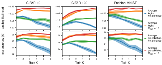
Figure 1: Comparison of averaging logits and probabilities for different values of $K_{\text{train}}$, and using $K_{\text{test}}=10$ vs. using no test-time augmentations. Here, we use ResNet18 with SGD (i.e. no Bayesian inference). We use only full orbit to decouple $K_{\text{train}}$ from $K_{\text{test}}$.

We trained ResNet18 on CIFAR-10, CIFAR-100 (Krizhevsky et al.,, 2009) and FashionMNIST (Xiao et al.,, 2017) with a learning rate of 0.1, decayed to 0.01 three quarters of the way through training. We apply two augmentation transformations: 1. a random crop with padding of four pixels, on all borders and 2. a random horizontal flip with probability 0.5. The training runs took around 12 GPU-days on Nvidia 2080s.

In agreement with past work (Lyle et al.,, 2020), we found that averaging over augmentations at test-time (red and orange) is better than using the test image without augmentation (green and blue), with $K_{\text{train}}=1$ corresponding to the standard DA procedure. In addition, we show that improved performance with multiple test-time augmentations continues to hold for larger values of $K_{\text{train}}$. Thus, if sufficient compute is available at test-time, averaging across augmentations gives an easy method to improve the performance of a pre-trained network.

Importantly, we see some performance gains with higher values of $K_{\text{train}}$ if we focus on the case with test augmentations, though they are somewhat inconsistent across datasets. We see strong improvements for the hardest dataset (CIFAR-100), and smaller improvements that saturate at $K_{\text{train}}=2$ for CIFAR-10. For FashionMNIST, the picture is more mixed. We suspect this is because we used a DA strategy tuned for CIFAR-10 and CIFAR-100, rather than FashionMNIST.

In addition, averaging probabilities seems to give somewhat better performance than averaging logits: compare averaging probabilities vs. logits both with test-time augmentation (red vs. orange) and without test-time augmentation (green vs. blue). The performance differences are consistent in both comparisons, though smaller when test-time augmentation is applied.

Indeed, performance falls quite dramatically as $K_{\text{train}}$ increases for averaging logits without test-time augmentation (blue). This is an indication that averaging probabilities and logits might actually behave quite differently. To understand how these differences might arise, consider the effect of averaging on the NN function itself. Both schemes can be justified by using averaging to increase invariance to the augmentation transformations (Sec. 3.2). Averaging probabilities, however, also forces the NN function itself to become invariant. If different augmentations produce different predictions, then the resulting averaged prediction will be more uncertain, which is penalized by the likelihood on the training points. This effect is much weaker when averaging logits. Consider an extreme example, as illustrated in Fig. 2. It is a two-class classification problem with two augmentations, $\mathbf{x}^{\prime}_{1}$ and $\mathbf{x}^{\prime}_{2}$, of the same image with logits, $\mathbf{f}(\mathbf{x}^{\prime}_{1})=(10,-10)$ and $\mathbf{f}(\mathbf{x}^{\prime}_{2})=(-1,1)$. Averaging logits gives us $\operatorname{\mathbb{E}}\left[\mathbf{f}(\mathbf{x}^{\prime})\right]=(4.5,-4.5)$, and applying the softmax, we very confidently predict the first class. In contrast, if we use averaging probabilities, then the first augmentation almost certainly predicts the first class $p(\mathbf{x}^{\prime}_{1})\approx(1,0)$ and the second augmentation almost certainly predicts the second class, $p(\mathbf{x}^{\prime}_{2})\approx(0,1)$, so when we average them we obtain $\operatorname{\mathbb{E}}\left[p(\mathbf{x}^{\prime})\right]\approx(0.5,0.5)$, which indicates a high degree of uncertainty.

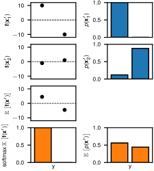
Figure 2: Example effect of averaging logits against averaging probabilities. $\mathbf{x}^{\prime}_{1}$ and $\mathbf{x}^{\prime}_{2}$ are two augmentations of the same image, $\mathbf{f}(\mathbf{x}^{\prime}_{1})$ and $\mathbf{f}(\mathbf{x}^{\prime}_{2})$ are logits outputted by a NN, and $p(\mathbf{x}^{\prime}_{1})$ and $p(\mathbf{x}^{\prime}_{2})$ are the probabilities corresponding to these logits. The prediction derived from the averaged logits is much more certain than the average of the individual probabilities.

4.2 Bayesian neural networks and the cold posterior effect

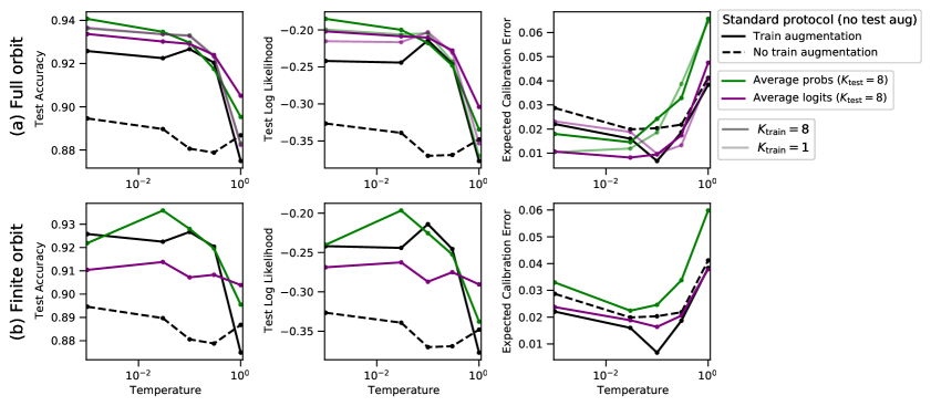
Figure 3: The cold posterior effect for different DA setups when running GGMC with ResNet20 on CIFAR-10. Without DA, there is a minimal CPE. Most other configurations show significant improvement for $T<1$, with the exception of averaging the logits over a finite orbit. Averages computed with $K_{\text{train}}=8$ and $K_{\text{test}}=8$.

Next, we ask a very different question: how is the CPE influenced when DA is incorporated into the model in a principled way? To this end, we use a different experimental setup. In particular, we take the code and networks from Fortuin et al., 2021b ; Fortuin et al., 2021a and mirror their experimental setup as closely as possible. This code combines a cyclical learning rate schedule (Zhang et al.,, 2019), a gradient-guided Monte Carlo (GGMC) scheme (Garriga-Alonso and Fortuin,, 2021), and the preconditioning and convergence diagnostics from Wenzel et al., (2020). The DA transformations are the same as those described in Sec. 4.1. Following Fortuin et al., 2021b , we ran 60 cycles with 50 epochs in each cycle. We recorded one sample at the end of each of the last five epochs of a cycle, giving 300 samples total. Importantly, to allow for running many sampling epochs in these experiments, we follow Fortuin et al., 2021b in using the ResNet20 architecture from Wenzel et al., (2020), which has far fewer channels than the ResNet18 used in Sec. 4.1 (i.e. 32 channels for the first block up to 128 in the last block compared to 64 channels up to 512 (He et al., 2016a, )). As such, SGD in this network performs poorly compared with that in Sec. 4.1 ($\sim 92\%$ (Wenzel et al.,, 2020) vs. $\sim 95\%$ (He et al., 2016b, )). The experiments took around 60 GPU-days on Nvidia RTX6000s.

The results are presented in Fig. 3. We replicate the finding that the CPE is largely absent without DA (dashed black line), and is present in the standard setup with DA at training time ($K_{\text{train}}=1$) but without augmentation at test time (solid black). Further, we show that the CPE persists with principled DA likelihoods: averaging logits with full orbit (purple, top row), and averaging probabilities with finite and full orbits (green). The best method overall appears to be averaging probabilities with a full orbit (dark green line, top row) at $T=0.001$, though averaging logits (dark purple lines) is better at $T=1$.

Surprisingly, the CPE is absent in one particular setting: averaging logits with a finite orbit (dashed purple line). However, the relevance of this is unclear, as it is clearly the worst performing of all our approaches by quite some margin. Indeed, remember that the arguments for the optimality of Bayesian inference apply only in the case that the model is well-specified (Kolmogorov,, 1950; Savage,, 1954; Jaynes,, 2003). However, the poor performance of averaging logits with a finite orbit indicates that it is likely to be the wrong model, while other settings are likely to be closer to the true model. In that case, the presence or absence of the CPE in the wrong model (averaging logits with a finite orbit) is immaterial to our understanding of the CPE in the right model. See also Sec. 6; note that this argument could not be made if there was a model without the CPE with performance equal to or better than the other models.

The CPE was originally discovered in Wenzel et al., (2020) when assessing test accuracy and log-likelihood — they did not consider other measures of distribution calibration like ECE. Indeed, later work on the cold posterior effect found that measures such as ECE are far more complex and usually do not agree with test accuracy and log-likelihood (Fortuin et al., 2021a, ). It is therefore difficult to interpret the differences between test log-likelihod and ECE, especially if we remember that test log-likelihood is itself a proper scoring rule (Gneiting and Raftery,, 2007), and therefore it does capture one possible notion of calibration. In particular, test log-likelihood heavily penalizes an event assessed as low probability actually happening, e.g. if our classifier predicts a probability of $0.001\%$, while the actually happens even $0.1\%$ of the time. In contrast, ECE considers the absolute difference in probability, so it far more heavily penalises e.g. a predicted probability of $40\%$ while the event actually happens $60\%$ of the time. Needless to say, the most appropriate measure of calibration will depend heavily on the domain, with log-likelihood being appropriate for low-probability but high risk events: in the example considered here of $0.001\%$ vs $0.1\%$, the factor of 100 error in the estimated probability could be catastrophic, despite representing a tiny absolute error of only $0.1\%-0.001\%=0.099\%$.

The usefulness of these results is contingent on understanding whether we are indeed accurately approximating the posterior. To check this, we computed the kinetic temperature (Leimkuhler and Matthews,, 2015), which estimates the temperature of a given parameter in the Langevin dynamics simulation from the norm of its momentum. In expectation, the kinetic temperature estimator should be equal to the desired temperature, $T$. The results (Appendix C) indicate that all the samplers run at their desired temperature, a result that is consistent with accurate posterior sampling.

As discussed in Sec. 3, increasing $K$ tightens our log-likelihood bounds. However, increasing $K$ also incurs greater computational cost. It is natural to question which value of $K$ is a good trade-off. To answer this, we explore how the log-likelihood of test data under a trained model varies with $K_{\text{test}}$. As expected, the results (Fig. 4) show the log-likelihood increases with $K_{\text{test}}$, with even $K=2$ being a significant improvement over $K=1$ (standard DA). Further, the curve plateaus, suggesting that for CIFAR-10, there is little benefit of using $K>8$.

5 RELATED WORK

Past work introduced generative models which average probabilities (Wenzel et al.,, 2020). However, this work did not consider the tight multi-sample bounds developed here, or the finite orbit setting which allows us to evaluate the exact likelihood. This left open the possibility raised by Izmailov et al., (2021) that the CPE was an artifact of standard DA resulting in an invalid likelihood. In contrast, we considered exact likelihoods in the finite orbit setting, and tight multi-sample lower bounds in the full orbit setting. As the CPE persists when using our exact likelihoods or tight lower bounds, we can exclude the possibility that the CPE is an artifact of DA giving a “randomly perturbed log-likelihood”. Other work has introduced a log-likelihood estimator for averaging GP logits (van der Wilk et al.,, 2018). However, the method only works for a quadratic log-likelihood and thus necessitates Pólya-Gamma approximations for classification. Further, the work did not consider BNNs or the connection to the CPE.

There is a small but growing body of work that considers averaging over multiple augmentations at training time (Hoffer et al.,, 2019; Berman et al.,, 2019; Choi et al.,, 2019; Benton et al.,, 2020; Lyle et al.,, 2020; Touvron et al.,, 2021). The issue is still highly topical, with important contemporaneous work (Fort et al.,, 2021). However, this work was not done within a Bayesian framework (e.g. by using stochastic gradient Langevin dynamics (SGLD) or a similar inference algorithm), did not show that averaging across multiple training augmentations gives a tight multi-sample bound on the log-likelihood of a principled model, did not consider the finite-orbit setting where the log-likelihood can be computed exactly, and did not consider the interaction with the CPE. In addition, much of this work uses averaging losses (Benton et al.,, 2020; Touvron et al.,, 2021; Fort et al.,, 2021) which is equivalent to using a loose single-sample bound on the log-likelihoods. Finally, the idea of averaging at test-time is more common and has been practiced for longer (e.g. Krizhevsky et al.,, 2012; Simonyan and Zisserman,, 2014; He et al.,, 2015; Szegedy et al.,, 2015; Foster et al.,, 2020).

A considerable body of past work on BNNs uses DA, both with variational inference (Blundell et al.,, 2015) and SGLD (e.g. Zhang et al.,, 2018, 2019; Osawa et al.,, 2019; Fortuin et al., 2021b, ; Immer et al.,, 2021). However, as discussed in Sec. 2 (Background), these methods simply substitute non-augmented for augmented data and thus do not use a valid log-likelihood. In contrast, we incorporated DA into the probabilistic generative model, and thus are able to give valid log-likelihoods based on averaging logits or averaging probabilities.

Figure 4: The effect of $K_{\text{test}}$ on the log-likelihood bound for a test batch (size 512) of CIFAR-10. Values shown for ResNet20 BNN trained and tested with $\hat{\mathcal{L}}_{\text{prob},K}$ ($K_{\text{train}}=8$ and $T=0.001$). Error bars cover two standard errors above/below mean for DA sampling with different seeds. Sixty seeds used for $K_{\text{test}}=\{1,2\}$, thirty for $K_{\text{test}}=4$ and five for all other $K_{\text{test}}$.

6 IMPLICATIONS FOR THE CPE

We have shown that the CPE persists even when using models incorporating principled DA, and in agreement with past work (Wenzel et al.,, 2020; Fortuin et al., 2021b, ; Izmailov et al.,, 2021), we show that the CPE disappears without DA.

What do these results imply for the origin of the CPE? First, our models in principle have a clean log-likelihood which can be evaluated exactly in the finite orbit setting, or which we estimate using tight multi-sample bounds in the full orbit setting. Thus, we can no longer dismiss the CPE as an artifact arising from DA giving a “randomly perturbed log-likelihood [which] does not have a clean interpretation as a valid likelihood function”.

Indeed, it is worth stepping back and considering the original motivation for studying the CPE, namely that if we have the correct model, then Bayesian inference with T=1 should give optimal performance (Kolmogorov,, 1950; Savage,, 1954; Jaynes,, 2003; Wenzel et al.,, 2020). Critically, we need the right model for us to expect optimal performance at T=1. We now have two classes of model, with DA and without DA, so which is right(er)? Given the significant and widely recognised performance benefits of DA, it seems very likely that the “right” model would include some form of DA. If the model with DA is right(er), and that model displays the CPE, then the CPE still demands an explanation, and the presence or absence of the CPE in the wrong model without DA is immaterial. As such, the presence of the CPE in models with DA remains an important problem, and is likely to be caused by one of the two other explanations discussed in Sec. 1 (Introduction): either data curation (Aitchison,, 2020) or prior misspecification (Wenzel et al.,, 2020; Fortuin et al., 2021b, ). Indeed, we would tentatively suggest the opposite of Izmailov et al., (2021): that it is in reality the lack of a CPE without DA that is an artifact of using the wrong model (i.e. without DA).

Finally, note that the CPE is not always observed, e.g. in language modelling (Izmailov et al.,, 2021). This is absolutely expected as the data-curation explanation of Aitchison, (2020) only implies CPE in fairly restricted settings; i.e. only in the case of reasonably accurate approximate posterior inference, such as SGLD, in a BNN where the data has been curated by excluding datapoints with an ambiguous class-label. Thus, Aitchison, (2020) does not lead us to expect the CPE e.g. in latent variable models, in regression settings (where you typically do not curate data), or in hybrid models where we perform Bayesian inference over only a small subset of parameters.

 

Supplementary material for data augmentation in Bayesian neural networks and the cold posterior effect

 

Appendix A AVERAGING LOSSES EMERGES WHEN USING DA IN VI AND SGLD

There are two particularly important algorithms for doing Bayesian inference in neural networks: stochastic gradient Langevin dynamics (SGLD; Welling and Teh,, 2011) and variational inference (VI; Blundell et al.,, 2015). In SGLD without DA, we draw samples from the posterior over weights by following gradient of the log-probability with added noise,

$$\left(\Delta\mathbf{w}\right)_{\text{noaug}}=\frac{\epsilon}{2}\nabla_{\mathbf{w}}\Bigg{[}\log\operatorname{P}\left(\mathbf{w}\right)+\sum_{i=1}^{N}\log\operatorname{P}_{\text{noaug}}\left(y_{i}\middle|\mathbf{x}_{i},\mathbf{w}\right)\Bigg{]}+\sqrt{\epsilon}\;\boldsymbol{\eta}$$ (19)

where $\boldsymbol{\eta}$ is standard Gaussian IID noise, and for simplicity we give the expression for full-batch Langevin dynamics rather than minibatched SGLD (they do not differ for the purposes of reasoning about DA). Likewise the variational inference objective is,

$$\text{ELBO}_{\text{noaug}}=\operatorname{\mathbb{E}}_{\operatorname{Q}\left(\mathbf{w}\right)}\Bigg{[}\log\operatorname{P}\left(\mathbf{w}\right)+\sum_{i=1}^{N}\log\operatorname{P}_{\text{noaug}}\left(y_{i}\middle|\mathbf{x}_{i},\mathbf{w}\right)-\log\operatorname{Q}\left(\mathbf{w}\right)\Bigg{]}$$ (20)

where $\operatorname{Q}\left(\mathbf{w}\right)$ is the variational approximate posterior learned by optimizing this objective. To understand the overall effect of this approach to DA, we replace $\log\operatorname{P}_{\text{noaug}}\left(y_{i}\middle|\mathbf{x}_{i},\mathbf{w}\right)$ with the log-softmax using (Eq. 4). Then, we consider the expected update to the weights, averaging over the augmented images, $\mathbf{x}_{i}^{\prime}$ conditioned on the underlying unaugmented images, $\mathbf{x}_{i}$,

$$\operatorname{\mathbb{E}}\left[\left(\Delta\mathbf{w}\right)_{\text{aug}}\right] =\frac{\epsilon}{2}\nabla_{\mathbf{w}}\Bigg{[}\log\operatorname{P}\left(\mathbf{w}\right)+\sum_{i=1}^{N}\mathcal{L}_{\text{loss}}^{i}\left(y_{i};\mathbf{w}\right)\Bigg{]}+\sqrt{\epsilon}\;\boldsymbol{\eta},$$ (21)

$$\text{ELBO}_{\text{aug}} =\operatorname{\mathbb{E}}_{\operatorname{Q}\left(\mathbf{w}\right)}\Bigg{[}\log\operatorname{P}\left(\mathbf{w}\right)+\sum_{i=1}^{N}\mathcal{L}_{\text{loss}}^{i}\left(y_{i};\mathbf{w}\right)-\log\operatorname{Q}\left(\mathbf{w}\right)\Bigg{]}.$$ (22)

In both cases, this ultimately replaces $\log\operatorname{P}_{\text{noaug}}\left(y_{i}\middle|\mathbf{x}_{i},\mathbf{w}\right)$ with $\mathcal{L}_{\text{loss}}^{i}\left(y_{i};\mathbf{w}\right)$, which as discussed in Sec. 3 is not a valid log-likelihood.

Appendix B THE APPROXIMATE POSTERIOR IN VI REDUCES VARIANCE

Here, we derive the ELBO using Jensen’s inequality; we take $x$ to be the data and $z$ to be a latent variable. Our goal is to compute the model evidence, $\operatorname{P}\left(x\right)$, by integrating out $z$,

$$\operatorname{P}\left(x\right) =\int dz\operatorname{P}\left(x\middle|z\right)\operatorname{P}\left(z\right)=\int dz\operatorname{P}\left(x,z\right)$$ (23)

where $\operatorname{P}\left(z\right)$ is the prior, $\operatorname{P}\left(x\middle|z\right)$ is the likelihood and $\operatorname{P}\left(x,z\right)$ is the joint. We introduce an approximate posterior, $\operatorname{Q}\left(z\right)$, and rewrite the integral as an expectation over that approximate posterior and apply Jensen’s inequality,

$$\log\operatorname{P}\left(x\right) =\log\int dz\operatorname{Q}\left(z\right)\frac{\operatorname{P}\left(x,z\right)}{\operatorname{Q}\left(z\right)}$$ (24)

$$=\log\operatorname{\mathbb{E}}_{\operatorname{Q}\left(z\right)}\left[\frac{\operatorname{P}\left(x,z\right)}{\operatorname{Q}\left(z\right)}\right]\geq\operatorname{\mathbb{E}}_{\operatorname{Q}\left(z\right)}\left[\log\frac{\operatorname{P}\left(x,z\right)}{\operatorname{Q}\left(z\right)}\right].$$ (25)

Now it is evident that the tightness of the bound is controlled by the variance of $\operatorname{P}\left(x,z\right)/\operatorname{Q}\left(z\right)$. Critically, if $\operatorname{Q}\left(z\right)$ matches the true posterior,

$$\operatorname{Q}\left(z\right) =\operatorname{P}\left(z\middle|x\right)\propto\operatorname{P}\left(x,z\right)$$ (26)

then $\operatorname{P}\left(x,z\right)/\operatorname{Q}\left(z\right)$ is constant (zero variance) and the bound is tight.

Appendix C KINETIC TEMPERATURE DIAGNOSTIC RESULTS

Figure 5: The evolution of the kinetic temperature diagnostic (Leimkuhler and Matthews,, 2015) throughout inference. Good agreement between the diagnostic temperature and intended temperature (in legend) suggests accurate inference.

Appendix D GENERALIZATION OUTSIDE OF CLASSIFICATION

We may be interested in generalizing the averaging logits and averaging probabilities ideas outside classification. For averaging probabilities, we use,

$$\operatorname{P}\left(y_{i}|\mathbf{x}_{i}\right) =\int d\mathbf{x}^{\prime}_{i}\operatorname{P}\left(y_{i}|\mathbf{x}_{i}^{\prime}\right)\operatorname{P}\left(\mathbf{x}_{i}^{\prime}|\mathbf{x}_{i}\right)=\operatorname{\mathbb{E}}\left[\operatorname{P}\left(y_{i}|\mathbf{x}_{i}^{\prime}\right)\right]$$ (27)

Intuitively, each augmentation forms one component of a (potentially infinite) mixture model over the outputs, $y_{i}$. Importantly, this expression makes no assumption about the support of distributions over $y_{i}$, so $y_{i}$ could be a finite set (classification), real-valued (regression), or anything else (a string, a graph, etc.) Note that directly applying a multi-sample estimator to (the logarithm of) (Eq. 27) gives us a log-likelihood lower bound as in (Eq. 15).

To generalize averaging logits, consider a situation where a distribution over an arbitrary $y_{i}$ is parameterized by a vector, $\mathbf{f}_{i}$ output by a neural network,

$$\operatorname{P}\left(y_{i}|\mathbf{x}\right) =\pi\left(y_{i};\mathbf{f}_{i}\right).$$ (28)

In the standard case with no augmentation, we would take $\mathbf{f}_{i}=\mathbf{f}(\mathbf{x}_{i};\mathbf{w})$, (where we take $\mathbf{f}_{i}$ as the specific vector for input $i$, and $\mathbf{f}(\cdot;\cdot)$ as a function represented by a neural network, that takes an image and weights and returns a vector). In the case with augmentation, we can average neural network outputs across different augmentations,

$$\mathbf{f}_{i} =\int d\mathbf{x}^{\prime}_{i}\operatorname{P}\left(\mathbf{x}_{i}^{\prime}|\mathbf{x}_{i}\right)\mathbf{f}(\mathbf{x}_{i}^{\prime};\mathbf{w})=\operatorname{\mathbb{E}}\left[\mathbf{f}(\mathbf{x}_{i}^{\prime};\mathbf{w})\right].$$ (29)

Note that in this case we need additional conditions for the multi-sample estimator to form a lower bound. In particular, we need $\log\pi\left(y_{i};\mathbf{f}_{i}\right)$ to be concave when treated as a function of $\mathbf{f}_{i}$ for a fixed $y_{i}$.

Appendix E PERSPECTIVES OF PROBABILISTIC DATA AUGMENTATION

Here we explore in depth the two general approaches to probabilistic data augmentation (Eq. 27) and (Eq. 29). We discuss their justifications in Sec. E.1 and E.2, and compare their properties in Sec. E.3.

E.1 Invariance construction

In the main text, we suggest two ways of incorporating data augmentation: 1) by averaging logits output by the neural network, and 2) by averaging the predicted probabilities. In classification, both of these methods can be justified by attempting to create a prediction that is more invariant to the transformations in the data augmentation.

When averaging logits, we aim to make the neural network mapping $\mathbf{f}:\mathbb{R}^{D}\to\mathbb{R}^{C}$ more invariant by averaging the outputs as in (Eq. 29). This construction influences only the regression function, and so has a similar effect to changing the neural network architecture or changing the prior on the functions $\mathbf{f}(\cdot)$ in the Bayesian case (van der Wilk et al.,, 2018). Since only the outputs are affected, this can be directly applied to any likelihood that depends only on an evaluation of the function, i.e. any likelihood which can be written as $\operatorname{P}(y_{i}|\mathbf{f}_{i})$.

In the case of averaging the probabilities, we can consider the model to be learning a mapping from image inputs to probability vectors $\mathbf{p}:\mathbb{R}^{D}\to\mathbb{P^{C}}$. We can make this mapping more invariant in the same way:

$$\mathbf{p}_{\text{inv}}(\mathbf{x}_{i};\mathbf{w}) =\operatorname{\mathbb{E}}\left[\operatorname{softmax}\left(\mathbf{f}(\mathbf{x}^{\prime}_{i};\mathbf{w})\right)\right]$$

$$=\int\operatorname{softmax}\left(\mathbf{f}(\mathbf{x}^{\prime}_{i};\mathbf{w})\right)\operatorname{P}(\mathbf{x}^{\prime}_{i}|\mathbf{x}_{i})\mathrm{d}\mathbf{x}^{\prime}_{i}\,.$$ (30)

The straightforward generalization of this construction would be to replace the softmax with the appropriate likelihood (see general case in (Eq. 27)). When considering likelihoods other than softmax classification (e.g. Gaussian likelihoods for regression), stronger differences between these constructions emerge in both behaviour and justification. We investigate further in Appendix E.3.

E.2 Noisy-input model

As stated above, we can generalize averaging the classification probabilities by replacing the softmax with the appropriate likelihood as in (Eq. 27). This modified likelihood, which incorporates data augmentation, was also discussed in Wenzel et al., (2020, Appendix K) and is a (potentially continuous) mixture model on the observation $y_{n}$, where each augmentation introduces a mixture component. This is as a noisy-input model (Girard and Murray-Smith,, 2003; McHutchon and Rasmussen,, 2011; Damianou et al.,, 2016) where the input $\mathbf{x}_{i}$ is corrupted via the augmentation distribution.

E.3 Model comparison

The forms of the invariance construction (Eq. 29) and the noisy-input model (Eq. 27) imply a difference of purpose. In using the invariance construction, we seek a regression function with the specified symmetry, which is consistent with the data according to the likelihood function $\operatorname{P}\left(y_{i}|\mathbf{f}_{i}\right)$. Conversely, with the noisy-input model (Eq. 27) we aim to find a function which gives rise to an invariant likelihood, consistent with the observed outputs for inputs randomly perturbed by $\operatorname{P}(\mathbf{x}^{\prime}|\mathbf{x})$. The role of $\mathbf{x}^{\prime}$ is different in each case. In the noisy-input model, $\mathbf{x}^{\prime}$ is a latent variable on which we could, in principle, do inference (with e.g. an amortized variational approach). While in the invariance construction, we integrate over $\mathbf{x}^{\prime}$ to parameterize $\mathbf{f}(\mathbf{x};\mathbf{w})$.

We now compare the behaviours of the invariance and noisy-input constructions. We will see that they result in quite different posteriors.

In the main text, we compared the empirical performance of averaging probabilities and averaging logits for BNN classification (see Figs. 1 and 3). However, as the invariance perspective justifies both averaging logits and probabilities, this comparison does not clearly distinguish between the noisy-input and invariance viewpoints. Further, we are interested not only in predictive performance but also in understanding how each construction behaves. With this in mind, we investigate the models with an illustrative example, where we can both integrate over the orbit and do inference in closed form.

(a) Invariant GP

(b) Noisy-input GP

(c) $p(y|x=4,\mathcal{D})$

Figure 6: Posterior densities for the model constructions for a single observation at $x_{1}=-4,y_{1}=2.5$.

We consider Gaussian process (GP) regression with a one-dimensional input and data augmentation which enforces symmetry about $x=0$, i.e. $\operatorname{P}(x^{\prime}|x)=\frac{1}{2}\left(\delta(x^{\prime}-x)+\delta(x^{\prime}+x)\right)$. From van der Wilk et al., (2018), the invariance view can be expressed in the kernel of the GP:

$$g \sim\mathcal{GP}(\mathbf{0},k_{\text{base}})$$ (31)

$$f(x) =g(x)+g(-x)$$ (32)

$$\implies f \sim\mathcal{GP}(\mathbf{0},k_{\text{inv}}),$$ (33)

$$\text{where}\hskip 15.0ptk_{\text{inv}}(x_{i},x_{j}) =\sum_{c_{i}\in\{-1,1\}}\sum_{c_{j}\in\{-1,1\}}k_{\text{base}}(c_{i}x_{i},c_{j}x_{j}).$$ (34)

We then follow standard GP inference to find the posterior over invariant functions. Note that unlike van der Wilk et al., (2018), we are not concerned with learning invariances here.

$$\operatorname{P}(\mathbf{x},\mathbf{y},\mathbf{f}) =\operatorname{P}(\mathbf{f})\prod_{i=1}^{N}\int\operatorname{P}(y_{i}|f(x_{i}^{\prime}))\operatorname{P}(x_{i}^{\prime}|x_{i})dx_{i}^{\prime}$$ (35)

$$\operatorname{P}(y_{i}|f(x_{i}^{\prime})) =\mathcal{N}\left(y_{i};f(x_{i}^{\prime}),\sigma^{2}\right)$$ (36)

$$f \sim\mathcal{GP}(0,k).$$ (37)

Given a single observation $$(x_{1},y_{1})$$, the noisy-input posterior is

$$\operatorname{P}(f|x_{1},y_{1}) =\frac{1}{Z}\operatorname{P}(f(x_{1}),x_{1},y_{1})$$ (38)

$$=\frac{1}{2Z}\operatorname{P}\left(f(x_{1})\right)\left[\operatorname{P}(y_{1}|f(x_{1}))+\operatorname{P}(y_{1}|f(-x_{1}))\right]$$ (39)

$$=\frac{1}{2}\left[\operatorname{P}(f|x_{1},y_{1})+\operatorname{P}(f|-x_{1},y_{1})\right],$$ (40)

a mixture of GP posteriors, with two components (one for each point in the orbit).

How do these posteriors compare? For an observation at $(x_{1}=-4,y_{1}=2.5)$ we plot the posterior predictive densities in Fig. 6. Both posteriors are symmetric around $x=0$ as we expect, however the noisy-input model is bimodal in the regions surrounding $x=4$ and $x=-4$, where the invariance posterior has unimodal density concentrated around the observed $y$ value of 2.5. The difference is clear in Fig. 6(c), which shows the marginal predictive densities at $x=4$.

Figure 7: Samples from the model posteriors. The red dot marks the location of the observation $(x_{1}=-4,y_{1}=2.5)$. The noisy input posterior comprises two components: one conditioned on $(x_{1},y_{1})$ (dashed lines), the other on $(-x_{1},y_{1})$ (solid lines).

In the noisy-input case, our observation is $(x_{1},y_{1})$, but $x$ is uncertain, so the observation could have been generated by $(-x_{1},y_{1})$ with equal probability. This results in a mixture posterior with two components: one component has “seen” $(x_{1},y_{1})$, while the other “saw” $(-x_{1},y_{1})$. The first component’s prediction at $-x_{1}$ remains uninformed by its “observation” and the same is true for the second component’s prediction at $x_{1}$. Thus, the predictions made by these components at these locations revert to the zero-mean prior.

From the invariance perspective, we condition on the point $(x_{1},y_{1})$ but the double-sum kernel forces the function to be the same at $(-x_{1},y_{1})$. As the posterior is a single GP, it has unimodal marginals with high density around both points.

We can gain further intuition by looking at samples from both posteriors (Fig. 7). We can see that the every sample from the invariance posterior is symmetric about $x=0$, where the functions drawn from the noisy input posterior are not symmetric in general.

The samples illustrate the key difference between the models. For the noisy input model, we can see the two components of the mixture posterior arise from conditioning on different locations in the orbit of $x_{1}$ as described above. The component going through $(x=4,y_{1})$ (samples drawn with dashed lines) is close to the prior at $(x=-4,y_{1})$, the other (solid lines) goes through $(x=-4,y_{1})$ and is close to the prior at $(x=4,y_{1})$. However, under the invariance model, inference on the observation concentrates all model density around $y_{1}$ for both points in the orbit of $x_{1}$.

We now consider how this comparison changes as we observe more data. The noisy-input model (Eq. 35) requires integration over $\operatorname{P}(x^{\prime}|x)$ to compute the likelihood of each datapoint, all of which are multiplied together to calculate their combined likelihood. Thus, the number of posterior components grows exponentially with the number of observations: $A^{N}$ (for orbit size $A$). Suppose all observations are at the same location $(x_{1},y_{1})$. In this case, the posterior density due to prior reversion at $\{x_{1},-x_{1}\}$ decreases exponentially with $N$. This is because the fraction of mixture components conditioned on all input observations being at the same point in the orbit of $x_{1}$, i.e. all at $x_{1}$ or $-x_{1}$, is given by $A^{1-N}$. The predictive posteriors for ten observations, each at $(x=-4,y=2.5)$ is shown in Fig. 8. Contrasting this noisy-input posterior (Fig. 8(b)) to that for one observation (Fig. 6(b)), we can see the reduction in density around to the prior mean for points around the orbit of $x_{1}$. In summary, the noisy-input and invariance posteriors become more alike as we observe more data in the same orbit.

(a) Invariant GP

(b) Noisy-input GP

(c) $p(y|x=4,\mathcal{D})$

Figure 8: Posterior densities for the model constructions for ten observations at $\{(x_{i}=-4,y_{i}=2.5)\}_{i=1}^{10}$.

References

- Adlam et al., (2020) Adlam, B., Snoek, J., and Smith, S. L. (2020). Cold posteriors and aleatoric uncertainty. arXiv preprint arXiv:2008.00029.
- Aitchison, (2020) Aitchison, L. (2020). A statistical theory of cold posteriors in deep neural networks. arXiv preprint arXiv:2008.05912.
- Benton et al., (2020) Benton, G., Finzi, M., Izmailov, P., and Wilson, A. G. (2020). Learning invariances in neural networks. arXiv preprint arXiv:2010.11882.
- Berman et al., (2019) Berman, M., Jégou, H., Vedaldi, A., Kokkinos, I., and Douze, M. (2019). Multigrain: a unified image embedding for classes and instances. arXiv preprint arXiv:1902.05509.
- Bishop, (2006) Bishop, C. M. (2006). Pattern recognition and machine learning. springer.
- Blundell et al., (2015) Blundell, C., Cornebise, J., Kavukcuoglu, K., and Wierstra, D. (2015). Weight uncertainty in neural network. In International Conference on Machine Learning, pages 1613–1622. PMLR.
- Boyd et al., (2004) Boyd, S., Boyd, S. P., and Vandenberghe, L. (2004). Convex optimization. Cambridge university press.
- Burda et al., (2015) Burda, Y., Grosse, R., and Salakhutdinov, R. (2015). Importance weighted autoencoders. arXiv preprint arXiv:1509.00519.
- Chen et al., (2020) Chen, S., Dobriban, E., and Lee, J. H. (2020). A group-theoretic framework for data augmentation. Journal of Machine Learning Research, 21(245):1–71.
- Choi et al., (2019) Choi, D., Passos, A., Shallue, C. J., and Dahl, G. E. (2019). Faster neural network training with data echoing. arXiv preprint arXiv:1907.05550.
- Damianou et al., (2016) Damianou, A. C., Titsias, M. K., and Lawrence, N. (2016). Variational inference for latent variables and uncertain inputs in gaussian processes.
- Dao et al., (2019) Dao, T., Gu, A., Ratner, A., Smith, V., De Sa, C., and Re, C. (2019). A kernel theory of modern data augmentation. In Chaudhuri, K. and Salakhutdinov, R., editors, Proceedings of the 36th International Conference on Machine Learning, volume 97 of Proceedings of Machine Learning Research, pages 1528–1537. PMLR.
- Deng et al., (2009) Deng, J., Dong, W., Socher, R., Li, L.-J., Li, K., and Fei-Fei, L. (2009). Imagenet: A large-scale hierarchical image database. In 2009 IEEE conference on computer vision and pattern recognition, pages 248–255. Ieee.
- Fort et al., (2021) Fort, S., Brock, A., Pascanu, R., De, S., and Smith, S. L. (2021). Drawing multiple augmentation samples per image during training efficiently decreases test error. arXiv preprint arXiv:2105.13343.
- (15) Fortuin, V., Garriga-Alonso, A., van der Wilk, M., and Aitchison, L. (2021a). BNNpriors: A library for Bayesian neural network inference with different prior distributions. Software Impacts, page 100079.
- (16) Fortuin, V., Garriga-Alonso, A., Wenzel, F., Rätsch, G., Turner, R., van der Wilk, M., and Aitchison, L. (2021b). Bayesian neural network priors revisited. arXiv preprint arXiv:2102.06571.
- Foster et al., (2020) Foster, A., Pukdee, R., and Rainforth, T. (2020). Improving transformation invariance in contrastive representation learning. arXiv preprint arXiv:2010.09515.
- Garriga-Alonso and Fortuin, (2021) Garriga-Alonso, A. and Fortuin, V. (2021). Exact Langevin dynamics with stochastic gradients. arXiv preprint arXiv:2102.01691.
- Ginsbourger et al., (2012) Ginsbourger, D., Bay, X., Roustant, O., and Carraro, L. (2012). Argumentwise invariant kernels for the approximation of invariant functions. In Annales de la Faculté des sciences de Toulouse: Mathématiques, volume 21, pages 501–527.
- Ginsbourger et al., (2013) Ginsbourger, D., Roustant, O., and Durrande, N. (2013). Invariances of random fields paths, with applications in Gaussian process regression. arXiv preprint arXiv:1308.1359.
- Girard and Murray-Smith, (2003) Girard, A. and Murray-Smith, R. (2003). Learning a gaussian process model with uncertain inputs. Department of Computing Science, University of Glasgow, Tech. Rep. TR-2003-144.
- Gneiting and Raftery, (2007) Gneiting, T. and Raftery, A. E. (2007). Strictly proper scoring rules, prediction, and estimation. Journal of the American statistical Association, 102(477):359–378.
- Grünwald, (2012) Grünwald, P. (2012). The safe bayesian. In International Conference on Algorithmic Learning Theory, pages 169–183. Springer.
- Grünwald et al., (2017) Grünwald, P., Van Ommen, T., et al. (2017). Inconsistency of bayesian inference for misspecified linear models, and a proposal for repairing it. Bayesian Analysis, 12(4):1069–1103.
- He et al., (2015) He, K., Zhang, X., Ren, S., and Sun, J. (2015). Delving deep into rectifiers: Surpassing human-level performance on ImageNet classification. In Proceedings of the IEEE international conference on computer vision, pages 1026–1034.
- (26) He, K., Zhang, X., Ren, S., and Sun, J. (2016a). Deep residual learning for image recognition. In Proceedings of the IEEE conference on computer vision and pattern recognition, pages 770–778.
- (27) He, K., Zhang, X., Ren, S., and Sun, J. (2016b). Identity mappings in deep residual networks. In European conference on computer vision, pages 630–645. Springer.
- Hoffer et al., (2019) Hoffer, E., Ben-Nun, T., Hubara, I., Giladi, N., Hoefler, T., and Soudry, D. (2019). Augment your batch: better training with larger batches. arXiv preprint arXiv:1901.09335.
- Immer et al., (2021) Immer, A., Bauer, M., Fortuin, V., Rätsch, G., and Khan, M. E. (2021). Scalable marginal likelihood estimation for model selection in deep learning. arXiv preprint arXiv:2104.04975.
- Izmailov et al., (2021) Izmailov, P., Vikram, S., Hoffman, M. D., and Wilson, A. G. (2021). What are Bayesian neural network posteriors really like? arXiv:2104.14421.
- Jaynes, (2003) Jaynes, E. T. (2003). Probability theory: The logic of science. Cambridge university press.
- Jordan et al., (1999) Jordan, M. I., Ghahramani, Z., Jaakkola, T. S., and Saul, L. K. (1999). An introduction to variational methods for graphical models. Machine learning, 37(2):183–233.
- Kolmogorov, (1950) Kolmogorov, A. (1950). Foundations of the theory of probability. Courier Dover Publications.
- Kondor, (2008) Kondor, I. R. (2008). Group theoretical methods in machine learning.
- Krizhevsky et al., (2009) Krizhevsky, A., Hinton, G., et al. (2009). Learning multiple layers of features from tiny images.
- Krizhevsky et al., (2012) Krizhevsky, A., Sutskever, I., and Hinton, G. E. (2012). ImageNet classification with deep convolutional neural networks. Advances in neural information processing systems, 25:1097–1105.
- Leimkuhler and Matthews, (2015) Leimkuhler, B. and Matthews, C. (2015). The canonical distribution and stochastic differential equations. In Molecular Dynamics, pages 211–260. Springer.
- Loosli et al., (2007) Loosli, G., Canu, S., and Bottou, L. (2007). Training invariant support vector machines using selective sampling. Large scale kernel machines, 2.
- Lyle et al., (2020) Lyle, C., van der Wilk, M., Kwiatkowska, M., Gal, Y., and Bloem-Reddy, B. (2020). On the benefits of invariance in neural networks. arXiv preprint arXiv:2005.00178.
- McHutchon and Rasmussen, (2011) McHutchon, A. and Rasmussen, C. (2011). Gaussian process training with input noise. Advances in Neural Information Processing Systems, 24:1341–1349.
- Noci et al., (2021) Noci, L., Roth, K., Bachmann, G., Nowozin, S., and Hofmann, T. (2021). Disentangling the roles of curation, data-augmentation and the prior in the cold posterior effect. arXiv preprint arXiv:2106.06596.
- Osawa et al., (2019) Osawa, K., Swaroop, S., Jain, A., Eschenhagen, R., Turner, R. E., Yokota, R., and Khan, M. E. (2019). Practical deep learning with Bayesian principles. arXiv preprint arXiv:1906.02506.
- Savage, (1954) Savage, L. J. (1954). The foundations of statistics. Courier Corporation.
- Simonyan and Zisserman, (2014) Simonyan, K. and Zisserman, A. (2014). Very deep convolutional networks for large-scale image recognition. arXiv preprint arXiv:1409.1556.
- Szegedy et al., (2015) Szegedy, C., Liu, W., Jia, Y., Sermanet, P., Reed, S., Anguelov, D., Erhan, D., Vanhoucke, V., and Rabinovich, A. (2015). Going deeper with convolutions. In Proceedings of the IEEE conference on computer vision and pattern recognition, pages 1–9.
- Touvron et al., (2021) Touvron, H., Cord, M., Sablayrolles, A., Synnaeve, G., and Jégou, H. (2021). Going deeper with image transformers. arXiv preprint arXiv:2103.17239.
- van der Wilk et al., (2018) van der Wilk, M., Bauer, M., John, S., and Hensman, J. (2018). Learning invariances using the marginal likelihood. arXiv preprint arXiv:1808.05563.
- Welling and Teh, (2011) Welling, M. and Teh, Y. W. (2011). Bayesian learning via stochastic gradient Langevin dynamics. In Proceedings of the 28th international conference on machine learning (ICML-11), pages 681–688. Citeseer.
- Wenzel et al., (2020) Wenzel, F., Roth, K., Veeling, B. S., Świątkowski, J., Tran, L., Mandt, S., Snoek, J., Salimans, T., Jenatton, R., and Nowozin, S. (2020). How good is the Bayes posterior in deep neural networks really? arXiv preprint arXiv:2002.02405.
- Xiao et al., (2017) Xiao, H., Rasul, K., and Vollgraf, R. (2017). Fashion-MNIST: a novel image dataset for benchmarking machine learning algorithms. arXiv preprint arXiv:1708.07747.
- Zhang et al., (2018) Zhang, G., Sun, S., Duvenaud, D., and Grosse, R. (2018). Noisy natural gradient as variational inference. In International Conference on Machine Learning, pages 5852–5861. PMLR.
- Zhang et al., (2019) Zhang, R., Li, C., Zhang, J., Chen, C., and Wilson, A. G. (2019). Cyclical stochastic gradient MCMC for Bayesian deep learning. arXiv preprint arXiv:1902.03932.