Aggregation before Generation: Factuality Controlled Text Generation

Planning to Aggregate Language

Planning to Aggregate in Language Generation

Planning to Aggregate in Data-to-Text Generation

Sentence Planning in Data-to-Text Generation

AggGen: Jointly learning sentence planning and realisation in data-to-text generation VR: Do we need to mention aggregation in the title cf. name of the system?

AggGen: Ordering and Aggregating while Generating

AggGen: Ordering and Aggregating while Generating

Abstract

We present AggGen (pronounced ‘again’) a data-to-text model which re-introduces two explicit sentence planning stages into neural data-to-text systems: input ordering and input aggregation. In contrast to previous work using sentence planning, our model is still end-to-end: AggGen performs sentence planning at the same time as generating text by learning latent alignments (via semantic facts) between input representation and target text. Experiments on the WebNLG and E2E challenge data show that by using fact-based alignments our approach is more interpretable, expressive, robust to noise, and easier to control, while retaining the advantages of end-to-end systems in terms of fluency. Our code is available at https://github.com/XinnuoXu/AggGen.

1 Introduction

Recent neural data-to-text systems generate text “end-to-end” (E2E) by learning an implicit mapping between input representations (e.g. RDF triples) and target texts. While this can lead to increased fluency, E2E methods often produce repetitions, hallucination and/or omission of important content for data-to-text Dušek et al. (2020) as well as other natural language generation (NLG) tasks Cao et al. (2018); Rohrbach et al. (2018). Traditional NLG systems, on the other hand, tightly control which content gets generated, as well as its ordering and aggregation. This process is called sentence planning Reiter and Dale (2000); Duboue and McKeown (2001, 2002); Konstas and Lapata (2013); Gatt and Krahmer (2018). Figure 1 shows two different ways to arrange and combine the representations in the input, resulting in widely different generated target texts.

In this work, we combine advances of both paradigms into a single system by reintroducing sentence planning into neural architectures. We call our system AggGen (pronounced ‘again’). AggGen jointly learns to generate and plan at the same time. Crucially, our sentence plans are interpretable latent states using semantic facts (obtained via Semantic Role Labelling (SRL)) that align the target text with parts of the input representation. In contrast, the plan used in other neural plan-based approaches is usually limited in terms of its interpretability, control, and expressivity. For example, in Moryossef et al. (2019b); Zhao et al. (2020) the sentence plan is created independently, incurring error propagation; Wiseman et al. (2018) use latent segmentation that limits interpretability; Shao et al. (2019) sample from a latent variable, not allowing for explicit control; and Shen et al. (2020) aggregate multiple input representations which limits expressiveness.

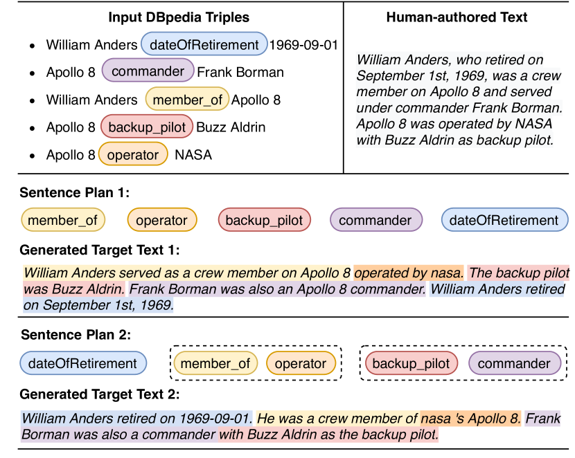
Figure 1: Two different sentence plans with their corresponding generated target texts from our model on the WebNLG dataset. Planning and generation is performed jointly. The dashed line denotes aggregation.

AggGen explicitly models the two planning processes (ordering and aggregation), but can directly influence the resulting plan and generated target text, using a separate inference algorithm based on dynamic programming. Crucially, this enables us to directly evaluate and inspect the model’s planning and alignment performance by comparing to manually aligned reference texts.

We demonstrate this for two data-to-text generation tasks: the E2E NLG Novikova et al. (2017) and the WebNLG Challenge Gardent et al. (2017a). We work with a triple-based semantic representation where a triple consists of a subject, a predicate and an object. For instance, in the last triple in Figure 1, Apollo 8, operator and NASA are the subject, predicate and object respectively. Our contributions are as follows:

$\bullet$ We present a novel interpretable architecture for jointly learning to plan and generate based on modelling ordering and aggregation by aligning facts in the target text to input representations with an HMM and Transformer encoder-decoder.

$\bullet$ We show that our method generates output with higher factual correctness than vanilla encoder-decoder models without semantic information.

$\bullet$ We also introduce an intrinsic evaluation framework for inspecting sentence planning with a rigorous human evaluation procedure to assess factual correctness in terms of alignment, aggregation and ordering performance.

2 Related Work

Factual correctness is one of the main issues for data-to-text generation: How to generate text according to the facts specified in the input triples without adding, deleting or replacing information?

The prevailing sequence-to-sequence (seq2seq) architectures typically address this issue via reranking Wen et al. (2015a); Dušek and Jurčíček (2016); Juraska et al. (2018) or some sophisticated training techniques Nie et al. (2019); Kedzie and McKeown (2019); Qader et al. (2019). For applications where structured inputs are present, neural graph encoders Marcheggiani and Perez-Beltrachini (2018); Rao et al. (2019); Gao et al. (2020) or decoding of explicit graph references Logan et al. (2019) are applied for higher accuracy. Recently, large-scale pretraining has achieved SoTA results on WebNLG by fine-tuning T5 Kale and Rastogi (2020b).

Several works aim to improve accuracy and controllability by dividing the end-to-end architecture into sentence planning and surface realisation. Castro Ferreira et al. (2019) feature a pipeline with multiple planning stages and Elder et al. (2019) introduce a symbolic intermediate representation in multi-stage neural generation. Moryossef et al. (2019b, a) use pattern matching to approximate the required planning annotation (entity mentions, their order and sentence splits). Zhao et al. (2020) use a planning stage in a graph-based model – the graph is first reordered into a plan; the decoder conditions on both the input graph encoder and the linearized plan. Similarly, Fan et al. (2019) use a pipeline approach for story generation via SRL-based sketches. However, all of these pipeline-based approaches either require additional manual annotation or depend on a parser for the intermediate steps.

Other works, in contrast, learn planning and realisation jointly. For example, Su et al. (2018) introduce a hierarchical decoding model generating different parts of speech at different levels, while filling in slots between previously generated tokens. Puduppully et al. (2019) include a jointly trained content selection and ordering module that is applied before the main text generation step.The model is trained by maximizing the log-likelihood of the gold content plan and the gold output text. Li and Rush (2020) utilize posterior regularization in a structured variational framework to induce which input items are being described by each token of the generated text. Wiseman et al. (2018) aim for better semantic control by using a Hidden Semi-Markov Model (HSMM) for splitting target sentences into short phrases corresponding to “templates”, which are then concatenated to produce the outputs. However it trades the controllability for fluency. Similarly, Shen et al. (2020) explicitly segment target text into fragment units, while aligning them with their corresponding input. Shao et al. (2019) use a Hierarchical Variational Model to aggregate input items into a sequence of local latent variables and realize sentences conditioned on the aggregations. The aggregation strategy is controlled by sampling from a global latent variable.

In contrast to these previous works, we achieve input ordering and aggregation, input-output alignment and text generation control via interpretable states, while preserving fluency.

3 Joint Planning and Generation

We jointly learn to generate and plan by aligning facts in the target text with parts of the input representation. We model this alignment using a Hidden Markov Model (HMM) that follows a hierarchical structure comprising two sets of latent states, corresponding to ordering and aggregation. The model is trained end-to-end and all intermediate steps are learned in a unified framework.

3.1 Model Overview

Let $x=\left\{x_{1},x_{2},\ldots,x_{J}\right\}$ be a collection of $J$ input triples and $\mathbf{y}$ their natural language description (human written target text). We first segment $\mathbf{y}$ into a sequence of $T$ facts $\mathbf{y}_{1:T}=\mathbf{y}_{1},\mathbf{y}_{2},\ldots,\mathbf{y}_{T}$, where each fact roughly captures “who did what to whom” in one event. We follow the approach of Xu et al. (2020), where facts correspond to predicates and their arguments as identified by SRL (See Appendix B for more details). For example:

Each fact $\mathbf{y}_{t}$ consists of a sequence of tokens $y_{t}^{1},y_{t}^{2},\ldots,y_{t}^{N_{t}}$. Unlike the text itself, the planning information, i.e. input aggregation and ordering, is not directly observable due to the absence of labelled datasets. AggGen therefore utilises an HMM probabilistic model which assumes that there is an underlying hidden process that can be modeled by a first-order Markov chain. At each time step, a latent variable (in our case input triples) is responsible for emitting an observed variable (in our case a fact text segment). The HMM specifies a joint distribution on the observations and the latent variables. Here, a latent state $\mathbf{z}_{t}$ emits a fact $\mathbf{y}_{t}$, representing the group of input triples that is verbalized in $\mathbf{y}_{t}$. We write the joint likelihood as:

$$\begin{split}p&\left(\mathbf{z}_{1:T},\mathbf{y}_{1:T}\mid x\right)=p\left(\mathbf{z}_{1:T}\mid x\right)p\left(\mathbf{y}_{1:T}\mid\mathbf{z}_{1:T},x\right)\\ &=\left[p\left(\mathbf{z}_{1}\mid x\right)\prod_{t=2}^{T}p\left(\mathbf{z}_{t}\mid\mathbf{z}_{t-1},x\right)\right]\left[\prod_{t=1}^{T}p\left(\mathbf{y}_{t}\mid\mathbf{z}_{t},x\right)\right].\end{split}$$

i.e., it is a product of the probabilities of each latent state transition (transition distribution) and the probability of the observations given their respective latent state (emission distribution).

3.2 Parameterization

Latent State.

A latent state $\mathbf{z}_{t}$ represents the input triples that are verbalized in the observed fact $\mathbf{y}_{t}$. It is not guaranteed that one fact always verbalizes only one triple (see bottom example in Figure 1). Thus, we represent state $\mathbf{z}_{t}$ as a sequence of latent variables $o_{t}^{1},\ldots,o_{t}^{L_{t}}$, where $L_{t}$ is the number of triples verbalized in $\mathbf{y}_{t}$. Figure 2 shows the structure of the model.

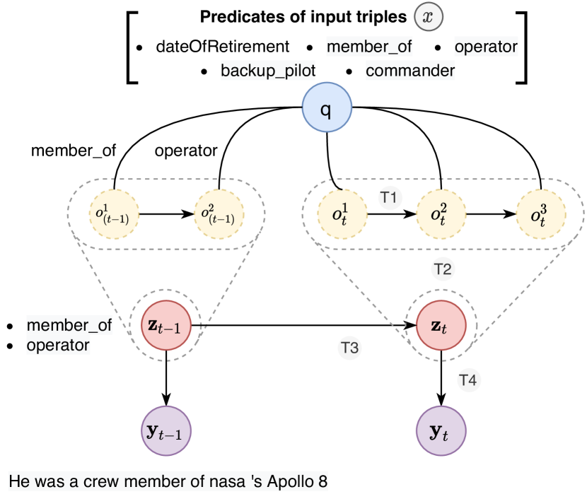
Figure 2: The structure of our model. $\mathbf{z}_{t}$, $\mathbf{z}_{t-1}$, $\mathbf{y}_{t}$, and $\mathbf{y}_{t-1}$ represent the basic HMM structure, where $\mathbf{z}_{t}$, $\mathbf{z}_{t-1}$ are latent states and $\mathbf{y}_{t}$, $\mathbf{y}_{t-1}$ are observations. Inside the dashed frames is the corresponding structure for each latent state $\mathbf{z}_{t}$, which is a sequence of latent variables $\mathbf{o}_{t}^{L_{t}}$ representing the predicates that emit the observation. For example, at time step $t-1$ two input triples (‘member_of’ and ‘operator’) are verbalized in the observed fact $\mathbf{y}_{t-1}$, whose predicates are represented as latent variables $o_{(t-1)}^{1}$ and $o_{(t-1)}^{2}$. T1–4 represent transitions introduced in Section 3.2.

Let $o_{t}^{l}\in\mathbb{Q}=\left\{1,\ldots,K\right\}$ be a set of possible latent variables, then $K^{L_{t}}$ is the size of the search space for $\mathbf{z}_{t}$. If $o_{t}^{l}$ maps to unique triples, the search space becomes intractable for a large value of $K$. To make the problem tractable, we decrease $K$ by representing triples by their predicate. $\mathbb{Q}$ thus stands for the collection of all predicates appearing in the corpus. To reduce the search space for $\mathbf{z}_{t}$ further, we limit $L_{t}<\mathbb{L}$, where $\mathbb{L}=3$.

Transition Distribution.

The transition distribution between latent variables (T1 in Figure 2) is a $K\times K$ matrix of probabilities, where each row sums to 1. We define this matrix as

$$p\left(o_{t}^{l}\mid o_{t}^{(l-1)},x\right)=\textup{softmax}\left(AB\odot M\left(q\right)\right)$$ (1)

where $\odot$ denotes the Hadamard product. $A\in\mathbb{R}^{K\times m}$ and $B\in\mathbb{R}^{m\times K}$ are matrices of predicate embeddings with dimension $m$. $q=\left\{q_{1},q_{2},\ldots,q_{J}\right\}$ is the set of predicates of the input triples $x$, and each $q_{j}\in\mathbb{Q}$ is the predicate of the triple $x_{j}$. $M\left(q\right)$ is a ${K\times K}$ masking matrix, where $M_{ij}=1$ if $i\in q$ and $j\in q$, otherwise $M_{ij}=0$. We apply row-wise softmax over the resulting matrix to obtain probabilities.

The probability of generating the latent state $\mathbf{z}_{t}$ (T2 in Figure 2) can be written as the joint distribution of the latent variables $o_{t}^{1},\ldots,o_{t}^{L_{t}}$. Assuming a first-order Markov chain, we get:

$$\begin{split}p\left(\mathbf{z}_{t}\mid x\right)&=p\left(o_{t}^{0},o_{t}^{1},o_{t}^{2},\ldots,o_{t}^{L_{t}}\mid x\right)\\ &=p\left(o_{t}^{0}\mid x\right)\left[\prod_{l=1}^{L_{t}}p\left(o_{t}^{l}\mid o_{t}^{(l-1)},x\right)\right],\end{split}\vspace{-6pt}$$

where $o_{t}^{0}$ is a marked start-state.

On top of the generation probability of the latent states $p\left(\mathbf{z}_{t}\mid x\right)$ and $p\left(\mathbf{z}_{t-1}\mid x\right)$, we define the transition distribution between two latent states (T3 in Figure 2) as:

$$\begin{split}p\left(\mathbf{z}_{t}\mid\mathbf{z}_{t-1},x\right)=&p\left(o_{(t-1)}^{0},\ldots,o_{(t-1)}^{L_{t-1}}\mid x\right)\\ &\cdot p\left(o_{t}^{1}\mid o_{(t-1)}^{L_{t-1}},x\right)\\ &\cdot p\left(o_{t}^{0},\ldots,o_{t}^{L_{t}}\mid x\right),\end{split}$$

where $o_{(t-1)}^{L_{t-1}}$ denotes the last latent variable in latent state $\mathbf{z}_{t-1}$, while $o_{t1}$ denotes the first latent variable (other than the start-state) in latent state $\mathbf{z}_{t}$. We use two sets of parameters $\left\{A_{\textup{in}},B_{\textup{in}}\right\}$ and $\left\{A_{\textup{out}},B_{\textup{out}}\right\}$ to describe the transition distribution between latent variables within and across latent states, respectively.

Emission Distribution.

The emission distribution $p\left(\mathbf{y}_{t}\mid\mathbf{z}_{t},x\right)$ (T4 in Figure 2) describes the generation of fact $\mathbf{y}_{t}$ conditioned on latent state $\mathbf{z}_{t}$ and input triples $x$. We define the probability of generating a fact as the product over token-level probabilities,

$$\begin{split}p\left(\mathbf{y}_{t}\mid\mathbf{z}_{t},x\right)=p(y_{t}^{1}\mid\mathbf{z}_{t},x)\prod_{i=2}^{N_{t}}p(y_{t}^{i}\mid y_{t}^{1:(i-1)},\mathbf{z}_{t},x).\end{split}\vspace{-12pt}$$

The first and last token of a fact are marked fact-start and fact-end tokens. We adopt Transformer Vaswani et al. (2017) as the model’s encoder and decoder.

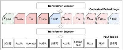
Figure 6: The Transformer encoder takes linearized triples and produces contextual embeddings We assume that, at time step $t$, the Transformer decoder is generating fact $\mathbf{y}_{t}$ conditioned on $\mathbf{z}_{t}$. The number of latent variables $L_{t}$ is 1. In other words, $\mathbf{z}_{t}=o_{t1}$. If the value of $o_{t1}$ is the predicate of the first triple (solid borders), then the second triple (dashed borders) is masked out for the encoder-decoder attention during decoding.

Each triple is linearized into a list of tokens following the order: subject, predicate, and object. In order to represent individual triples, we insert special [SEP] tokens at the end of each triple. A special [CLS] token is inserted before all input triples, representing the beginning of the entire input. An example where the encoder produces a contextual embedding for the tokens of two input triples is shown in Figure 6 in Appendix E.

At time step $t$, the decoder generates fact $\mathbf{y}_{t}$ token-by-token autoregressively, conditioned on both the contextually-encoded input and the latent state $\mathbf{z}_{t}$. To guarantee that the generation of $\mathbf{y}_{t}$ conditions only on the input triples whose predicate is in $\mathbf{z}_{t}$, we mask out the contextual embeddings of tokens from other unrelated triples for the encoder-decoder attention in all Transformer layers.

Autoregressive Decoding.

Autoregressive Hidden Markov Model (AR-HMM) introduces extra links into HMM to capture long-term correlations between observed variables, i.e., output tokens. Following Wiseman et al. (2018), we use AR-HMM for decoding, therefore allowing the interdependence between tokens to generate more fluent and natural text descriptions. Each token distribution depends on all the previously generated tokens, i.e., we define the token-level probabilities as $p(y_{t}^{i}\mid y_{1:(t-1)}^{1:N_{t}},y_{t}^{1:(i-1)},\mathbf{z}_{t},x)$ instead of $p(y_{t}^{i}\mid y_{t}^{1:(i-1)},\mathbf{z}_{t},x)$. During training, at each time step $t$, we teacher-force the generation of the fact $\mathbf{y}_{t}$ by feeding the ground-truth history, $\mathbf{y}_{1:(t-1)}$, to the word-level Transformer decoder. However, since only $\mathbf{y}_{t}$ depends on the current hidden state $\mathbf{z}_{t}$, we only calculate the loss over $\mathbf{y}_{t}$.

3.3 Learning

We apply the backward algorithm Rabiner (1989) to learn the parameters introduced in Section 3.2, where we maximize $p(\mathbf{y}\mid x)$, i.e., the marginal likelihood of the observed facts $\mathbf{y}$ given input triples $x$, over all the latent states $\mathbf{z}$ and $\mathbf{o}$ on the entire dataset using dynamic programming. Following Murphy (2012), and given that the latent state at time $t$ is $C$, we define a conditional likelihood of future evidence as:

$$\begin{split}\beta_{t}\left(C\right)\triangleq p\left(\mathbf{y}_{t+1:T}\mid\mathbf{z}_{t}=C,x\right),\end{split}$$ (2)

where $C$ denotes a group of predicates that are associated with the emission of $\mathbf{y}$. The size of $C$ ranges from 1 to $\mathbb{L}$ and each component is from the collection of predicates $\mathbb{Q}$ (see Section 3.2). Then, the backward recurrences are:

$$\begin{split}&\beta_{t-1}\left({C}^{\prime}\right)=p\left(\mathbf{y}_{t:T}\mid\mathbf{z}_{t-1}={C}^{\prime},x\right)\\ &=\sum_{C}\beta_{t}\left(C\right)p\left(\mathbf{y}_{t}\mid\mathbf{z}_{t}=C,x\right)p\left(\mathbf{z}_{t}=C\mid\mathbf{z}_{t-1}={C}^{\prime},x\right)\end{split}$$

with the base case $\beta_{T}\left(C\right)=1$. The marginal probability of $\mathbf{y}$ over latent $\mathbf{z}$ is then obtained as $p\left(\mathbf{y}\mid x\right)=\sum_{C}\beta_{0}\left(C\right)p\left(\mathbf{z}_{1}=C|x\right)$.

In Equation 2, the size of the search space for $C$ is $\sum_{\alpha=1}^{\mathbb{L}}K^{\alpha}$, where $K=\left|\mathbb{Q}\right|$, i.e., the number of unique predicates appearing in the dataset. The problem can still be intractable due to high $K$, despite the simplifications explained in Section 3.2 (cf. predicates). To tackle this issue and reduce the search space of $C$, we: (1) only explore permutations of $C$ that include predicates appearing on the input; (2) introduce a heuristic based on the overlap of tokens between a triple and a fact—if a certain fact mentions most tokens appearing in the predicate and object of a triple we hard-align it to this triple. As a result, we discard the permutations that do not include the aligned predicates.

3.4 Inference

After the joint learning process, the model is able to plan, i.e., order and aggregate the input triples in the most likely way, and then generate a text description following the planning results. Therefore, the joint prediction of $(\hat{y},\hat{\mathbf{z}})$ is defined as:

$$\begin{split}\left(\hat{y},\hat{\mathbf{z}}\right)&=\underset{\left(\mathbf{y}^{\prime},\mathbf{z}^{\prime}\right),\mathbf{z}^{\prime}\in\{\tilde{\mathbf{z}}^{(i)}\}}{\operatorname{arg}\,\operatorname{max}}\;p\left(\mathbf{y}^{\prime},\mathbf{z}^{\prime}\mid x\right)\\ &=\underset{\left(\mathbf{y}^{\prime},\mathbf{z}^{\prime}\right),\mathbf{z}^{\prime}\in\{\tilde{\mathbf{z}}^{(i)}\}}{\operatorname{arg}\,\operatorname{max}}\;p(\mathbf{y}^{\prime}\mid\mathbf{z}^{\prime},x)p(\mathbf{z}^{\prime}\mid x),\end{split}\vspace{-4pt}$$ (3)

where $\{\tilde{\mathbf{z}}^{(i)}\}$ denotes a set of planning results, $\hat{y}$ is the text description, and $\hat{\mathbf{z}}$ is the planning result that $\hat{y}$ is generated from.

The entire inference process (see Figure 3) includes three steps: input ordering, input aggregation, and text generation. The first two steps are responsible for the generation of $\{\tilde{\mathbf{z}}^{(i)}\}$ together with their probabilities $\{p(\tilde{\mathbf{z}}^{(i)}\mid x)\}$, while the last step is for the text generation $p(\mathbf{y}^{\prime}\mid\tilde{\mathbf{z}}^{(i)},x)$.

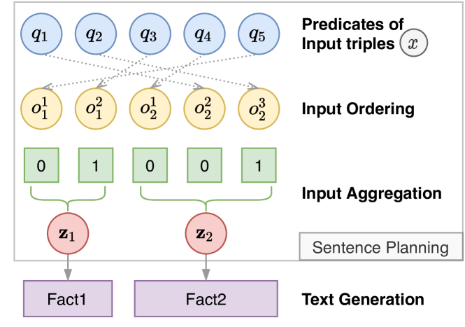
Figure 3: The inference process (Section 3.4)

Planning: Input Ordering. The aim is to find the top-k most likely orderings of predicates appearing in the input triples. In order to make the search process more efficient, we apply left-to-right beam-search based on the transition distribution introduced in Equation 1. Specifically, we use a transition distribution between latent variables within latent states, calculated with predicate embeddings $A_{\textup{in}}$ and $B_{\textup{in}}$ (see Section 3.2). To guarantee that the generated sequence does not suffer from omission and duplication of predicates, we constantly update the masking matrix $M(q)$ by removing generated predicates from the set $q$. The planning process stops when $q$ is empty.

Planning: Input Aggregation. The goal is to find the top-$n$ most likely aggregations for each result of the Input Ordering step. To implement this process efficiently, we introduce a binary state for each predicate in the sequence: 0 indicates “wait” and 1 indicates “emit” (green squares in Figure 3). Then we list all possible combinations of the binary states for the Input Ordering result. For each combination, the aggregation algorithm proceeds left-to-right over the predicates and groups those labelled as “emit” with all immediately preceding predicates labelled as “wait”. In turn, we rank all the combinations with the transition distribution introduced in Equation 1. In contrast to the Input Ordering step, we use the transition distribution between latent variables across latent states, calculated with predicate embeddings $A_{\textup{out}}$ and $B_{\textup{out}}$. That is, we do not take into account transitions between two consecutive predicates if they belong to the same group. Instead, we only consider consecutive predicates across two connected groups, i.e., the last predicate of the previous group with the first predicate of the following group.

Text Generation. The final step generates a text description conditioned on the input triples and the planning result (obtained from the Input Aggregation step). We use beam search and the planning-conditioned generation process described in Section 3.2 (“Emission Distribution”).

3.5 Controllability over sentence plans

While the jointly learnt model is capable of fully automatic generation including the planning step (see Section 3.4), the discrete latent space allows direct access to manually control the planning component, which is useful in settings which require increased human supervision and is a unique feature of our architecture. The plans (latent variables) can be controlled in two ways: (1) hyperparameter. Our code offers a hyperparameter that can be tuned to control the level of aggregation: no aggregation, aggregate one, two triples, etc. The model can predict the most likely plan based on the input triples and the hyperparameter and generate a corresponding text description; (2) the model can directly adopt human-written plans, e.g. using the notation [eatType][near customer-rating], which translates to: first generate ‘eatType’ as an independent fact and then aggregate the predicates ‘near’ and ‘customer-rating’ in the following fact and generate their joint description.

4 Experiments

4.1 Datasets

We tested our approach on two widely used data-to-text tasks: the E2E NLG Novikova et al. (2017) and WebNLG Gardent et al. (2017a). Compared to E2E, WebNLG is smaller, but contains more predicates and has a larger vocabulary. Statistics with examples can be found in Appendix C. We followed the original training-development-test data split for both datasets.

4.2 Evaluation Metrics

Generation Evaluation focuses on evaluating the generated text with respect to its similarity to human-authored reference sentences. To compare to previous work, we adopt their associated metrics to evaluate each task. The E2E task is evaluated using BLEU Papineni et al. (2002), NIST Doddington (2002), ROUGE-L Lin (2004), METEOR Lavie and Agarwal (2007), and CIDEr Vedantam et al. (2015). WebNLG is evaluated in terms of BLEU, METEOR, and TER Snover et al. (2006).

Factual Correctness Evaluation tests if the generated text corresponds to the input triples Wen et al. (2015b); Reed et al. (2018); Dušek et al. (2020). We evaluated on the E2E test set using automatic slot error rate (SER), i.e., an estimation of the occurrence of the input attributes (predicates) and their values in the outputs, implemented by Dušek et al. (2020). SER counts predicates that were added, missed or replaced with a wrong object.

Intrinsic Planning Evaluation examines planning performance in Section 6.

4.3 Baseline model and Training Details

To evaluate the contributions of the planning component, we choose the vanilla Transformer model Vaswani et al. (2017) as our baseline, trained on pairs of linearized input triples and target texts. In addition, we choose two types of previous works for comparison: (1) best-performing models reported on the WebNLG 2017 (seen) and E2E dataset, i.e. T5 Kale and Rastogi (2020b), PlanEnc Zhao et al. (2020), ADAPT Gardent et al. (2017b), and TGen Dušek and Jurčíček (2016); (2) models with explicit planning, i.e. TILB-PIPE Gardent et al. (2017b), NTemp+AR Wiseman et al. (2018) and Shen et al. (2020).

To make our HMM-based approach converge faster, we initialized its encoder and decoder with the baseline model parameters and fine-tuned them during training of the transition distributions. Encoder and decoder parameters were chosen based on validation results of the baseline model for each task (see Appendix D for details).

5 Experiment Results

5.1 Generation Evaluation Results

Model	BLEU	TER	METEOR
T5◆	64.70	—	0.46
PlanEnc◆	64.42	0.33	0.45
ADAPT◆	60.59	0.37	0.44
TILB-PIPE◆	44.34	0.48	0.38
Transformer	58.47	0.37	0.42
AggGen	58.74	0.40	0.43
AggGen${}_{-\textup{OD}}$	55.30	0.44	0.43
AggGen${}_{-\textup{AG}}$	52.17	0.50	0.44

Table 1: Generation Evaluation Results on the WebNLG (seen). The models labelled with ^◆ are from previous work. The rest are our implementations.

Model	BLEU	NIST	MET	R-L	CIDer	Add	Miss	Wrong	SER
TGen◆	66.41	8.5565	45.07	69.17	2.2253	00.14	04.11	00.03	04.27
NTemp+AR◆	59.80	7.5600	38.75	65.01	1.9500	—	—	—	—
Shen et al. (2020)◆	65.10	—	45.50	68.20	2.2410	—	—	—	—
Transformer	68.23	8.6765	44.31	6̱9.88	2.2153	00.30	04.67	00.20	05.16
AggGen	64.14	8.3509	45.13	66.62	2.1953	00.32	01.66	00.71	02.70
AggGen${}_{-\textup{OD}}$	58.90	7.9100	43.21	62.12	1.9656	01.65	02.99	03.01	07.65
AggGen${}_{-\textup{AG}}$	44.00	6.0890	43.75	58.24	0.8202	08.74	00.45	00.92	10.11

Table 2: Evaluation of Generation (middle) and Factual correctness (right) trained/tested on the original E2E data (Section 5 for metrics description). Models with ^◆ are from previous work, the rest are our implementations.

Table 1 shows the generation results on the WebNLG seen category Gardent et al. (2017b). Our model outperforms TILB-PIPE and Transformer, but performs worse than T5, PlanEnc and ADAPT. However, unlike these three models, our approach does not rely on large-scale pretraining, extra annotation, or heavy pre-processing using external resources. Table 2 shows the results when training and testing on the original E2E set. AggGen outperforms NTemp+AR and is comparable with Shen et al. (2020), but performs slightly worse than both seq2seq models in terms of word-overlap metrics.

However, the results in Table 3 demonstrate that our model does outperform the baselines on most surface metrics if trained on the noisy original E2E training set and tested on clean E2E data Dušek et al. (2019). This suggests that the previous performance drop was due to text references in the original dataset that did not verbalize all triples or added information not present in the triples that may have down-voted the fact-correct generations. This also shows that AggGen produces correct outputs even when trained on a noisy dataset. Since constructing high-quality data-to-text training sets is expensive and labor-intensive, this robustness towards noise is important.

Model	BLEU	NIST	MET	R-L	CIDer
TGen◆	39.23	6.022	36.97	55.52	1.762
Transformer	38.57	5.756	35.92	55.45	1.668
AggGen	41.06	6.207	37.91	55.13	1.844
AggGen${}_{-\textup{OD}}$	38.24	5.951	36.56	51.53	1.653
AggGen${}_{-\textup{AG}}$	30.44	4.636	37.99	49.94	0.936

Table 3: Evaluation of Generation trained on the original E2E data, while tested on the cleaned E2E data. Note that, the clean test set has more diverse MRs and fewer references per MR, which leads to lower scores – see also the paper introducing the cleaned E2E data (Table 2 and 3 in Dušek et al. (2019)).

5.2 Factual Correctness Results

The results for factual correctness evaluated using SER on the original E2E test set are shown in Table 2. The SER of AggGen is the best among all models. Especially, the high “Miss” scores for TGen and Transformer demonstrate the high chance of information omission in vanilla seq2seq-based generators. In contrast, AggGen shows much better coverage over the input triples while keeping a low level of hallucination (low “Add” and “Wrong” scores).

5.3 Ablation variants

To explore the effect of input planning on text generation, we introduced two model variants: AggGen${}_{-\textup{OD}}$, where we replaced the Input Ordering with randomly shuffling the input triples before input aggregation, and AggGen${}_{-\textup{AG}}$, where the Input Ordering result was passed directly to the text generation and the text decoder generated a fact for each input triple individually.

The generation evaluation results on both datasets (Table 1 and Table 2) show that AggGen outperforms AggGen${}_{-\textup{OD}}$ and AggGen${}_{-\textup{AG}}$ substantially, which means both Input Ordering and Input Aggregation are critical. Table 2 shows that the factual correctness results for the ablative variants are much worse than full AggGen, indicating that planning is essential for factual correctness. An exception is the lower number of missed slots in AggGen${}_{-\textup{AG}}$. This is expected since AggGen${}_{-\textup{AG}}$ generates a textual fact for each triple individually, which decreases the possibility of omissions at the cost of much lower fluency. This strategy also leads to a steep increase in added information.

Additionally, AggGen${}_{-\textup{AG}}$ performs even worse on the E2E dataset than on the WebNLG set. This result is also expected, since input aggregation is more pronounced in the E2E dataset with a higher number of facts and input triples per sentence (cf. Appendix C).

5.4 Qualitative Error Analysis

We manually examined a sample of 100 outputs (50 from each dataset) with respect to their factual correctness and fluency. For factual correctness, we follow the definition of SER and check whether there are hallucinations, substitutions or omissions in generated texts. For fluency, we check whether the generated texts suffer from grammar mistakes, redundancy, or contain unfinished sentences. Figure 4 shows two examples of generated texts from Transformer and AggGen (more examples, including target texts generated by AggGen${}_{-\textup{OD}}$ and AggGen${}_{-\textup{AG}}$, are shown in Table 6 and Table 7 in Appendix A). We observe that, in general, the seq2seq Transformer model tends to compress more triples into one fluent fact, whereas AggGen aggregates triples in more but smaller groups, and generates a shorter/simpler fact for each group. Therefore, the texts generated by Transformer are more compressed, while AggGen’s generations are longer with more sentences. However, the planning ensures that all input triples will still be mentioned. Thus, AggGen generates texts with higher factual correctness without trading off fluency.

Figure 4: Examples of input and system-generated target text for E2E (top) and WebNLG (bottom). The sequences in square brackets are the sentence plans.

6 Intrinsic Evaluation of Planning

We now directly inspect the performance of the planning component by taking advantage of the readability of SRL-aligned facts. In particular, we investigate: (1) Sentence planning performance. We study the agreement between model’s planning and reference planning for the same set of input triples; (2) Alignment performance – we use AggGen as an aligner and examine its ability to align segmented facts to the corresponding input triples. Since both studies require ground-truth triple-to-fact alignments, which are not part of the WebNLG and E2E data, we first introduce a human annotation process in Section 6.1.

6.1 Human-annotated Alignments

We asked crowd workers on Amazon Mechanical Turk to align input triples to their fact-based text snippets to derive a “reference plan” for each target text. Each worker was given a set of input triples and a corresponding reference text description, segmented into a sequence of facts. The workers were then asked to select the triples that are verbalised in each fact. We sampled 100 inputs from the WebNLG test set for annotation. Each input was paired with three reference target texts from WebNLG. To guarantee the correctness of the annotation, three different workers annotated each input-reference pair. We only consider the alignments where all three annotators agree. Using Fleiss Kappa Fleiss (1971) over the facts aligned by each judge to each triple, we obtained an average agreement of 0.767 for the 300 input-reference pairs, which is considered high agreement.

6.2 Study of Sentence Planning

We now check the agreement between the model-generated and reference plans based on the top-1 Input Aggregation result (see Section 3.4). We introduce two metrics:

$\bullet$ Normalized Mutual Information (NMI) Strehl and Ghosh (2002) to evaluate aggregation. We represent each plan as a set of clusters of triples, where a cluster contains the triples sharing the same fact verbalization. Using NMI we measure mutual information between two clusters, normalized into the 0-1 range, where 0 and 1 denote no mutual information and perfect correlation, respectively.

$\bullet$ Kendall’s tau ($\tau$) Kendall (1945) is a ranking based measure which we use to evaluate both ordering and aggregation. We represent each plan as a ranking of the input triples, where the rank of each triple is the position of its associated fact verbalization in the target text. $\tau$ measures rank correlation, ranging from -1 (strong disagreement) to 1 (strong agreement).

	$\textup{NMI}_{\textup{max}}$	$\textup{NMI}_{\textup{avg}}$	$\textup{K-tau}_{\textup{max}}$	$\textup{K-tau}_{\textup{avg}}$
Human	0.9340	0.7587	0.8415	0.2488
AggGen	0.7101	0.6247	0.6416	0.2064

Table 4: Planning Evaluation Results. NMI and K-tau calculated between human-written references (bottom), and between references and our system AggGen (top).

In the crowdsourced annotation (Section 6.1), each set of input triples contains three reference texts with annotated plans. We fist evaluate the correspondence among these three reference plans by calculating NMI and $\tau$ between one plan and the remaining two. In the top row of Table 4, the high average and maximum NMI indicate that the reference texts’ authors tend to aggregate input triples in similar ways. On the other hand, the low average $\tau$ shows that they are likely to order the aggregated groups differently. Then, for each set of input triples, we measure NMI and $\tau$ of the top-1 Input Aggregation result (model’s plan) against each of the corresponding reference plans and compute average and maximum values (bottom row in Table 4). Compared to the strong agreement among reference plans on the input aggregation, the agreement between model’s and reference plans is slightly weaker. Our model has slightly lower agreement on aggregation (NMI), but if we consider aggregation and ordering jointly ($\tau$), the agreement between our model’s plans and reference plans is comparable to the agreement among reference plans.

6.3 Study of Alignment

	Precision	Recall	F1
RB (%)	86.20	100.00	92.59
Vtb (%)	89.73	84.16	86.85

Table 5: Alignment Evaluation Results. Alignment accuracy for the Viterbi algorithm (Vtb) and the rule-based aligner (RB).

In this study, we use the HMM model as an aligner and assess its ability to align input triples with their fact verbalizations on the human-annotated set. Given the sequence of observed variables, a trained HMM-based model is able to find the most likely sequence of hidden states $\textbf{z}^{*}=\underset{\textbf{z}}{\arg\max}(\textbf{z}_{1:T}|\textbf{y}_{1:T})$ using Viterbi decoding. Similarly, given a set of input triples and a factoid segmented text, we use Viterbi with our model to align each fact with the corresponding input triple(s). We then evaluate the accuracy of the model-produced alignments against the crowdsourced alignments.

The alignment evaluation results are shown in Table 5. We compare the Viterbi (Vtb) alignments with the ones calculated by a rule-based aligner (RB) that aligns each triple to the fact with the greatest word overlap. The precision of the Viterbi aligner is higher than the rule-based aligner. However, the Viterbi aligner tends to miss triples, which leads to a lower recall. Since HMMs are locally optimal, the model cannot guarantee to annotate input triples once and only once.

7 Conclusion and Future Work

We show that explicit sentence planning, i.e., input ordering and aggregation, helps substantially to produce output which is both semantically correct as well as naturally sounding. Crucially, this also enables us to directly evaluate and inspect both the model’s planning and alignment performance by comparing to manually aligned reference texts. Our system outperforms vanilla seq2seq models when considering semantic accuracy and word-overlap based metrics. Experiment results also show that AggGen is robust to noisy training data. We plan to extend this work in three directions:

Other Generation Models. We plan to plug other text generators, e.g. pre-training based approaches Lewis et al. (2020); Kale and Rastogi (2020b) , into AggGen to enhance their interpretability and controllability via sentence planning and generation.

Zero/Few-shot scenarios. Kale and Rastogi (2020a)’s work on low-resource NLG uses a pre-trained language model with a schema-guided representation and hand-written templates to guide the representation in unseen domains and slots. These techniques can be plugged into AggGen, which allows us to examine the effectiveness of the explicit sentence planning in zero/few-shot scenarios.

Including Content Selection. In this work, we concentrate on the problem of faithful surface realization based on E2E and WebNLG data, which both operate under the assumption that all input predicates have to be realized in the output. In contrast, more challenging tasks such as RotoWire Wiseman et al. (2017), include content selection before sentence planning. In the future, we plan to include a content selection step to further extend AggGen’s usability.

Appendix A Examples of input and system-generated target text

Table 6: Examples of input and system-generated target text for E2E NLG dataset.

Input	the cricketers [customerrating] high
	the cricketers [eattype] restaurant
	the cricketers [near] express by holiday inn
Transf	Predicted Text: the cricketers is a highly rated restaurant near express by holiday inn.
AggGen	Sentence Planing: [eatType] [customerrating near]
	Predicted Text: the cricketers is a highly rated restaurant located near express by holiday inn.
AggGen${}_{-\textup{AG}}$	Sentence Planing: [eatType] [near] [customerrating]
	Predicted Text: the cricketers is a restaurant located near express by holiday inn . it has a high customer rating.
AggGen${}_{-\textup{OD}}$	Sentence Planing: [eatType near] [customerrating]
	Predicted Text: the cricketers is a restaurant near express by holiday inn . it has a high customer rating.
Input	blue spice [eattype] pub
	blue spice [familyfriendly] yes
	blue spice [food] english
	blue spice [near] rainbow vegetarian café
Transf	Predicted Text: the blue spice is a family friendly pub near the rainbow vegetarian café. it serves english food in the higher price range.
AggGen	Sentence Planing: [eatType familyFriendly] [food near]
	Predicted Text: blue spice is a family friendly pub serving english food near the rainbow vegetarian café.
AggGen${}_{-\textup{AG}}$	Sentence Planing: [eatType] [familyFriendly] [food] [near]
	Predicted Text: blue spice is a mid - priced pub that is family friendly and serves british food . it is located near the rainbow vegetarian café.
AggGen${}_{-\textup{OD}}$	Sentence Planing: [near familyFriendly eatType] [food]
	Predicted Text: blue spice is a family friendly pub near the rainbow vegetarian café . it serves english food.
Input	the cricketers [area] riverside
	the cricketers [customerrating] 5 out of 5
	the cricketers [eattype] restaurant
	the cricketers [familyfriendly] yes
	the cricketers [food] chinese
	the cricketers [near] all bar one
Transf	Predicted Text: the cricketers is a family friendly chinese restaurant near all bar one in the riverside area . it has a customer rating of 5 out of 5.
AggGen	Sentence Planing: [eatType familyFriendly] [food area near] [customerrating]
	Predicted Text: the cricketers is a family friendly chinese restaurant located in the riverside area near all bar one . it has a customer rating of 5 out of 5.
AggGen${}_{-\textup{AG}}$	Sentence Planing: [eatType] [food] [area] [customerrating] [familyFriendly] [near]
	Predicted Text: the cricketers is a restaurant that serves chinese food. it is located in the riverside area and has a customer rating of 5 out of 5 and is children friendly. the coffee shop is near all bar one.
AggGen${}_{-\textup{OD}}$	Sentence Planing: [customerrating] [familyFriendly eatType] [food near area]
	Predicted Text: the cricketers is a 5 out of 5 rated , family friendly chinese restaurant located in riverside near all bar one.
Input	the cricketers [area] city centre
	the cricketers [customerrating] average
	the cricketers [eattype] restaurant
	the cricketers [familyfriendly] yes
	the cricketers [food] chinese
	the cricketers [near] all bar one
	the cricketers [pricerange] high
Transf	Predicted Text: the cricketers is a chinese restaurant near all bar one in the city centre . it is children friendly and has an average customer rating.
AggGen	Sentence Planing: [eatType priceRange] [food customerrating] [familyFriendly area near]
	Predicted Text: the cricketers is a chinese restaurant with a high price range . it has an average customer rating and is children friendly near all bar one in the city centre.
AggGen${}_{-\textup{AG}}$	Sentence Planing: [eatType] [priceRange] [food] [customerrating] [familyFriendly] [area] [near]
	Predicted Text: the cricketers is a chinese restaurant that is children friendly, has a high price range, a customer rating of 3 out of 5, is located near the portland arms and is in the city centre. it has an average customer rating. is also a children-friendly . you can find it is called the cricketers.
AggGen${}_{-\textup{OD}}$	Sentence Planing: [area] [familyFriendly priceRange] [eatType food near] [customerrating]
	Predicted Text: located in the city centre, the cricketers is a child friendly chinese restaurant with a high price range. it is near all bar one. its customer rating is average.

Table 7: Examples of input and system-generated target text for WebNLG dataset.

Input	11th mississippi infantry monument [category] contributing property
	11th mississippi infantry monument [country] united states
	11th mississippi infantry monument [established] 2000
	11th mississippi infantry monument [location] seminary ridge
	11th mississippi infantry monument [municipality] gettysburg, pennsylvania
Transf	Predicted Text: the 11th mississippi infantry monument is located at seminary ridge, gettysburg, pennsylvania, united states. it was established in 2000 and falls under the category of contributing property.
AggGen	Sentence Planing: [location country established] [category] [municipality]
	Predicted Text: the 11th mississippi infantry monument, established in 2000, is located at seminary ridge, gettysburg, pennsylvania, united states. it is categorized as a contributing property and is in the municipality of gettysburg pennsylvania.
AggGen${}_{-\textup{AG}}$	Sentence Planing: [country] [established] [category] [municipality] [location]
	Predicted Text: the 11th mississippi infantry monument is located in gettysburg, pennsylvania, united states. the monument was established in 2000 and falls under the category of contributing property. it can be found in the municipality of gettysburg in pennsylvania and is in the seminary ridge.
AggGen${}_{-\textup{OD}}$	Sentence Planing: [municipality] [category] [country established] [location]
	Predicted Text: the 11th mississippi infantry monument is in the municipality of gettysburg, pennsylvania. it is categorized as a contributing property. the monument was established in the year 2000 in the united states and is located at seminary ridge.
Input	apollo 8 [backup_pilot] buzz aldrin
	apollo 8 [crewmembers] frank borman
	apollo 8 [operator] nasa
	william anders [birthplace] british hong kong
	william anders [dateofretirement] 1969-09-01
	william anders [was_a_crew_member_of] apollo 8
Transf	Predicted Text: william anders (born in british hong kong) was a crew member of nasa’s apollo 8 alongside frank borman. william anders retired on september 1st, 1969.
AggGen	Sentence Planing: [birthPlace] [was_a_crew_member_of] [operator crewMembers] [backup_pilot] [dateOfRetirement]
	Predicted Text: william anders was born in british hong kong and served as a crew member on apollo 8. frank borman was a crewman aboard the nasa operated apollo 8 mission. the backup pilot was buzz aldrin. william anders retired on september 1st, 1969.
AggGen${}_{-\textup{AG}}$	Sentence Planing: [birthPlace] [was_a_crew_member_of] [operator] [crewMembers] [backup_pilot] [dateOfRetirement]
	Predicted Text: william anders (born in british hong kong) was a crew member of apollo 8 operated by nasa, where buzz aldrin was a backup pilot. frank borman was also a crewman aboard apollo 8. buzz aldrin’s backup pilot was buzz aldrin. william anders retired on september 1st, 1969.
AggGen${}_{-\textup{OD}}$	Sentence Planing: [backup_pilot] [was_a_crew_member_of] []birthPlace] [dateOfRetirement operator] [crewMembers]
	Predicted Text: buzz aldrin was a crew member of apollo 8 with buzz aldrin as backup pilot and frank borman as buzz aldrin. william anders was a crewman aboard apollo 8. british hong kong born william anders retired. he was a backup pilot on the apollo 8 mission was operated by nasa. frank borman was also a crewman.
Input	school of business and social sciences at the aarhus university [affiliation] european university association
	school of business and social sciences at the aarhus university [city] aarhus
	school of business and social sciences at the aarhus university [country] denmark
	school of business and social sciences at the aarhus university [dean] thomas pallesen
	school of business and social sciences at the aarhus university [established] 1928
	school of business and social sciences at the aarhus university [latinname] universitas aarhusiensis
	school of business and social sciences at the aarhus university [numberofstudents] 16000
Transf	Predicted Text: the school of business and social sciences at the aarhus university in aarhus, denmark was established in 1928. it has 737 academic staff and 16,000 students. its dean is thomas pallesen and it is affiliated with the european university association.
AggGen	Sentence Planing: [country established city] [affiliation latinName numberOfStudents] [dean]
	Predicted Text: the school of business and social sciences at the aarhus university in aarhus, denmark was established in 1928. it has 737 academic staff and 16,000 students. its latin name is ”universitas aarhusiensis” and it is affiliated with the european university association. its dean is thomas pallesen.
AggGen${}_{-\textup{AG}}$	Sentence Planing: [country] [established] [city] [affiliation] [latinName] [numberOfStudents] [dean]
	Predicted Text: the school of business and social sciences at the aarhus university in denmark is affiliated with the european university association in brussels. the school was established in 1928 and is located in the city of aarhus. it is affiliated to the european univerrsity in the school the latin name of ”universitas aarhusiensis”. and there are 16000 students. its dean is thomas pallesen”.
AggGen${}_{-\textup{OD}}$	Sentence Planing: [latinName numberOfStudents] [country established] [dean affiliation] [city]
	Predicted Text: the school of business and social sciences at the aarhus university in aarhus, denmark has 16,000 students and its latin name is ”universitas aarhusiensis”. it was established in 1928 in the country of denmark and it is affiliated with the european university association. the current dean is thomas pallesen and it has strong connections with the school also affiliated to its dean of business. and it also home to the school.

Appendix B Factoid Sentence Segmentation

In order to align meaningful parts of the human-written target text to semantic triples, we first segment the target sentences into sequences of facts using SRL, following Xu et al. (2020). The aim is to break down sentences into sub-sentences (facts) that verbalize as few input triples as possible; the original sentence can still be fully recovered by concatenating all its sub-sentences. Each fact is represented by a segment of the original text that roughly captures “who did what to whom” in one event. We first parse the sentences into SRL propositions using the implementation of He et al. (2018). We consider each predicate-argument structure as a separate fact, where the predicate stands for the event and its arguments are mapped to actors, recipients, time, place, etc. (see Figure 5). The sentence segmentation consists of two consecutive steps:

(1) Tree Construction, where we construct a hierarchical tree structure for all the facts of one sentence, by choosing the fact with the largest coverage as the root and recursively building sub-trees by replacing arguments with their corresponding sub-facts (ARG1 in FACT1 is replaced by FACT2).

(2) Argument Grouping, where each predicate (FACT in tree) with its leaf-arguments corresponds to a sub-sentence. For example, in Figure 5, leaf-argument “was” and “a crew member on Apollo 8” of FACT1 are grouped as one sub-sentence.

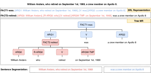
Figure 5: Semantic Role Labeling based tree meaning representation and factoid sentence segmentation for text “William Anders, who retired on September 1st, 1969, was a crew member on Apollo 8.”

Appendix C Datasets

WebNLG.

The corpus contains 21K instances (input-text pairs) from 9 different domains (e.g., astronauts, sports teams). The number of input triples ranges from 1 to 7, with an average of 2.9. The average number of facts that each text contains is 2.4 (see Appendix B). The corpus contains 272 distinct predicates. The vocabulary size for input and output side is 2.6K and 5K respectively.

E2E NLG.

The corpus contains 50K instances from the restaurant domain. We automatically convert the original attribute-value pairs to triples: For each instance, we take the restaurant name as the subject and use it along with the remaining attribute-value pairs as corresponding predicates and objects. The number of triples in each input ranges from 1 to 7 with an average of 4.4. The average number of facts that each text contains is 2.6. The corpus contains 9 distinct predicates. The vocabulary size for inputs and outputs is 120 and 2.4K respectively. We also tested our approach on an updated cleaned release Dušek et al. (2019).

Appendix D Hyperparameters

WebNLG.

Both encoder and decoder are a 2-layer 4-head Transformer, with hidden dimension of 256. The size of token embeddings and predicate embeddings is 256 and 128, respectively. The Adam optimizer Kingma and Ba (2015) is used to update parameters. For both the baseline model and the pre-train of the HMM-based model, the learning rate is 0.1. During the training of the HMM-based model, the learning rate for the encoder-decoder fine-tuning and the training of the transition distributions is set as 0.002 and 0.01, respectively.

E2E.

Both encoder and decoder are a Transformer with hidden dimension of 128. The size of token embeddings and predicate embeddings is 128 and 32, respectively. The rest hyper-parameters are same with WebNLG.

Appendix E Parameterization: Emission Distribution

Appendix F Full Experiment Results on E2E

Model	Train	Test	BLEU	NIST	MET	R-L	CIDer	Add	Miss	Wrong	SER
TGen◆	Original	Clean	39.23	6.0217	36.97	55.52	1.7623	00.40	03.59	00.07	04.05
Transformer			38.57	5.7555	35.92	55.45	1.6676	02.13	05.71	00.51	08.35
AggGen			41.06	6.2068	37.91	55.13	1.8443	02.04	03.38	00.64	06.06
AggGen${}_{-\textup{OD}}$			38.24	5.9509	36.56	51.53	1.6525	02.94	03.67	02.18	08.80
AggGen${}_{-\textup{AG}}$			30.44	4.6355	37.99	49.94	0.9359	08.71	01.60	00.87	11.24
TGen◆	Clean	Clean	40.73	6.1711	37.76	56.09	1.8518	00.07	00.72	00.08	00.87
Transformer			38.62	6.0804	36.03	54.82	1.7544	03.15	04.56	01.32	09.02
AggGen			39.88	6.1704	37.35	54.03	1.8193	01.10	01.85	01.25	04.21
AggGen${}_{-\textup{OD}}$			38.28	6.0027	36.94	51.55	1.6397	01.74	02.74	00.62	05.11
AggGen${}_{-\textup{AG}}$			26.92	4.2877	36.60	47.95	0.9205	05.99	01.54	02.31	09.98

Table 8: Evaluation of Generation (middle) and Factual correctness (right) on the E2E NLG data (see Section 5 for metrics decription).

Appendix G Annotation interface

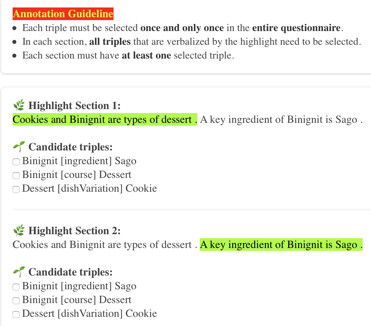
Figure 7: An example of the fact-triple alignment task (highlights correspond to facts).

References

- Cao et al. (2018) Ziqiang Cao, Furu Wei, Wenjie Li, and Sujian Li. 2018. Faithful to the Original: Fact Aware Neural Abstractive Summarization. In AAAI, New Orleans, LA, USA. ArXiv: 1711.04434.
- Castro Ferreira et al. (2019) Thiago Castro Ferreira, Chris van der Lee, Emiel van Miltenburg, and Emiel Krahmer. 2019. Neural data-to-text generation: A comparison between pipeline and end-to-end architectures. In 2019 Conference on Empirical Methods in Natural Language Processing (EMNLP) and 9th International Joint Conference on Natural Language Processing (IJCNLP), Hong Kong.
- Doddington (2002) George Doddington. 2002. Automatic evaluation of machine translation quality using n-gram co-occurrence statistics. In Proceedings of the second international conference on Human Language Technology Research, pages 138–145.
- Duboue and McKeown (2002) Pablo Duboue and Kathleen McKeown. 2002. Content planner construction via evolutionary algorithms and a corpus-based fitness function. In Proceedings of the International Natural Language Generation Conference, pages 89–96, Harriman, New York, USA. Association for Computational Linguistics.
- Duboue and McKeown (2001) Pablo A. Duboue and Kathleen R. McKeown. 2001. Empirically estimating order constraints for content planning in generation. In Proceedings of the 39th Annual Meeting of the Association for Computational Linguistics, pages 172–179, Toulouse, France. Association for Computational Linguistics.
- Dušek et al. (2019) Ondřej Dušek, David M. Howcroft, and Verena Rieser. 2019. Semantic noise matters for neural natural language generation. In Proc. of the 12th International Conference on Natural Language Generation, pages 421–426, Tokyo, Japan. Association for Computational Linguistics.
- Dušek and Jurčíček (2016) Ondřej Dušek and Filip Jurčíček. 2016. Sequence-to-sequence generation for spoken dialogue via deep syntax trees and strings. In Proceedings of the 54th Annual Meeting of the Association for Computational Linguistics (Volume 2: Short Papers), pages 45–51, Berlin, Germany. Association for Computational Linguistics.
- Dušek et al. (2020) Ondřej Dušek, Jekaterina Novikova, and Verena Rieser. 2020. Evaluating the State-of-the-Art of End-to-End Natural Language Generation: The E2E NLG Challenge. Computer Speech & Language, 59:123–156.
- Dušek and Jurčíček (2016) Ondřej Dušek and Filip Jurčíček. 2016. Sequence-to-Sequence Generation for Spoken Dialogue via Deep Syntax Trees and Strings. In Proceedings of the 54th Annual Meeting of the Association for Computational Linguistics (Volume 2: Short Papers), pages 45–51, Berlin. Association for Computational Linguistics.
- Dušek et al. (2020) Ondřej Dušek, Jekaterina Novikova, and Verena Rieser. 2020. Evaluating the state-of-the-art of end-to-end natural language generation: The e2e nlg challenge. Computer Speech & Language, 59:123 – 156.
- Elder et al. (2019) Henry Elder, Jennifer Foster, James Barry, and Alexander O’Connor. 2019. Designing a symbolic intermediate representation for neural surface realization. In Proceedings of the Workshop on Methods for Optimizing and Evaluating Neural Language Generation, pages 65–73, Minneapolis, Minnesota. Association for Computational Linguistics.
- Fan et al. (2019) Angela Fan, Mike Lewis, and Yann Dauphin. 2019. Strategies for Structuring Story Generation. In Proceedings of the 57th Annual Meeting of the Association for Computational Linguistics, pages 2650–2660, Florence, Italy. Association for Computational Linguistics.
- Fleiss (1971) Joseph L Fleiss. 1971. Measuring nominal scale agreement among many raters. Psychological bulletin, 76(5):378.
- Gao et al. (2020) Hanning Gao, Lingfei Wu, Po Hu, and Fangli Xu. 2020. RDF-to-Text Generation with Graph-augmented Structural Neural Encoders. In Proceedings of the Twenty-Ninth International Joint Conference on Artificial Intelligence, pages 3030–3036, Yokohama, Japan.
- Gardent et al. (2017a) Claire Gardent, Anastasia Shimorina, Shashi Narayan, and Laura Perez-Beltrachini. 2017a. Creating training corpora for NLG micro-planners. In Proceedings of the 55th Annual Meeting of the Association for Computational Linguistics (Volume 1: Long Papers), pages 179–188, Vancouver, Canada. Association for Computational Linguistics.
- Gardent et al. (2017b) Claire Gardent, Anastasia Shimorina, Shashi Narayan, and Laura Perez-Beltrachini. 2017b. The WebNLG Challenge: Generating Text from RDF Data. In Proceedings of the 10th International Conference on Natural Language Generation, pages 124–133, Santiago de Compostela, Spain. Association for Computational Linguistics.
- Gatt and Krahmer (2018) Albert Gatt and Emiel Krahmer. 2018. Survey of the state of the art in natural language generation: Core tasks, applications and evaluation. Journal of Artificial Intelligence Research, 61:65–170.
- He et al. (2018) Luheng He, Kenton Lee, Omer Levy, and Luke Zettlemoyer. 2018. Jointly predicting predicates and arguments in neural semantic role labeling. In Proceedings of the 56th Annual Meeting of the Association for Computational Linguistics (Volume 2: Short Papers), pages 364–369, Melbourne, Australia.
- Juraska et al. (2018) Juraj Juraska, Panagiotis Karagiannis, Kevin K. Bowden, and Marilyn A. Walker. 2018. A Deep Ensemble Model with Slot Alignment for Sequence-to-Sequence Natural Language Generation. In Proceedings of the 2018 Conference of the North American Chapter of the Association for Computational Linguistics: Human Language Technologies, Volume 1 (Long Papers), pages 152–162, New Orleans, LA, USA.
- Kale and Rastogi (2020a) Mihir Kale and Abhinav Rastogi. 2020a. Template guided text generation for task-oriented dialogue. In Proceedings of the 2020 Conference on Empirical Methods in Natural Language Processing (EMNLP), pages 6505–6520, Online. Association for Computational Linguistics.
- Kale and Rastogi (2020b) Mihir Kale and Abhinav Rastogi. 2020b. Text-to-text pre-training for data-to-text tasks. In Proceedings of the 13th International Conference on Natural Language Generation, pages 97–102, Dublin, Ireland. Association for Computational Linguistics.
- Kedzie and McKeown (2019) Chris Kedzie and Kathleen McKeown. 2019. A Good Sample is Hard to Find: Noise Injection Sampling and Self-Training for Neural Language Generation Models. In INLG, Tokyo, Japan.
- Kendall (1945) Maurice G Kendall. 1945. The treatment of ties in ranking problems. Biometrika, pages 239–251.
- Kingma and Ba (2015) Diederik Kingma and Jimmy Ba. 2015. Adam: A Method for Stochastic Optimization. In Proceedings of the 3rd International Conference on Learning Representations, San Diego, CA, USA. ArXiv: 1412.6980.
- Konstas and Lapata (2013) Ioannis Konstas and Mirella Lapata. 2013. Inducing document plans for concept-to-text generation. In Proceedings of the 2013 Conference on Empirical Methods in Natural Language Processing, pages 1503–1514, Seattle, Washington, USA. Association for Computational Linguistics.
- Lavie and Agarwal (2007) Alon Lavie and Abhaya Agarwal. 2007. Meteor: An automatic metric for mt evaluation with high levels of correlation with human judgments. In Proceedings of the second workshop on statistical machine translation, pages 228–231.
- Lewis et al. (2020) Mike Lewis, Yinhan Liu, Naman Goyal, Marjan Ghazvininejad, Abdelrahman Mohamed, Omer Levy, Veselin Stoyanov, and Luke Zettlemoyer. 2020. BART: Denoising sequence-to-sequence pre-training for natural language generation, translation, and comprehension. In Proceedings of the 58th Annual Meeting of the Association for Computational Linguistics, pages 7871–7880, Online. Association for Computational Linguistics.
- Li and Rush (2020) Xiang Lisa Li and Alexander Rush. 2020. Posterior control of blackbox generation. In Proceedings of the 58th Annual Meeting of the Association for Computational Linguistics, pages 2731–2743, Online. Association for Computational Linguistics.
- Lin (2004) Chin-Yew Lin. 2004. Rouge: A package for automatic evaluation of summaries. In Text summarization branches out, pages 74–81.
- Logan et al. (2019) Robert Logan, Nelson F. Liu, Matthew E. Peters, Matt Gardner, and Sameer Singh. 2019. Barack’s Wife Hillary: Using Knowledge Graphs for Fact-Aware Language Modeling. In Proceedings of the 57th Annual Meeting of the Association for Computational Linguistics, pages 5962–5971, Florence, Italy. Association for Computational Linguistics.
- Marcheggiani and Perez-Beltrachini (2018) Diego Marcheggiani and Laura Perez-Beltrachini. 2018. Deep Graph Convolutional Encoders for Structured Data to Text Generation. In Proceedings of the 11th International Conference on Natural Language Generation, pages 1–9, Tilburg University, The Netherlands. Association for Computational Linguistics.
- Moryossef et al. (2019a) Amit Moryossef, Ido Dagan, and Yoav Goldberg. 2019a. Improving Quality and Efficiency in Plan-based Neural Data-to-Text Generation. In INLG, Tokyo, Japan.
- Moryossef et al. (2019b) Amit Moryossef, Yoav Goldberg, and Ido Dagan. 2019b. Step-by-Step: Separating Planning from Realization in Neural Data-to-Text Generation. In NAACL, Minneapolis, MN, USA.
- Murphy (2012) Kevin P Murphy. 2012. Machine learning: a probabilistic perspective. MIT press.
- Nie et al. (2019) Feng Nie, Jin-Ge Yao, Jinpeng Wang, Rong Pan, and Chin-Yew Lin. 2019. A simple recipe towards reducing hallucination in neural surface realisation. Florence, Italy.
- Novikova et al. (2017) Jekaterina Novikova, Ondřej Dušek, and Verena Rieser. 2017. The E2E dataset: New challenges for end-to-end generation. In Proceedings of the 18th Annual SIGdial Meeting on Discourse and Dialogue, pages 201–206, Saarbrücken, Germany. Association for Computational Linguistics.
- Papineni et al. (2002) Kishore Papineni, Salim Roukos, Todd Ward, and Wei-Jing Zhu. 2002. Bleu: a method for automatic evaluation of machine translation. In Proceedings of the 40th Annual Meeting of the Association for Computational Linguistics, pages 311–318, Philadelphia, Pennsylvania, USA. Association for Computational Linguistics.
- Puduppully et al. (2019) Ratish Puduppully, Li Dong, and Mirella Lapata. 2019. Data-to-text generation with content selection and planning. In Proceedings of the 33rd AAAI Conference on Artificial Intelligence, Honolulu, Hawaii.
- Qader et al. (2019) Raheel Qader, Francois Portet, and Cyril Labbe. 2019. Semi-Supervised Neural Text Generation by Joint Learning of Natural Language Generation and Natural Language Understanding Models. In INLG, Tokyo, Japan.
- Rabiner (1989) Lawrence R Rabiner. 1989. A tutorial on hidden Markov models and selected applications in speech recognition. Proceedings of the IEEE, 77(2):257–286.
- Rao et al. (2019) Jinfeng Rao, Kartikeya Upasani, Anusha Balakrishnan, Michael White, Anuj Kumar, and Rajen Subba. 2019. A Tree-to-Sequence Model for Neural NLG in Task-Oriented Dialog. In INLG, Tokyo, Japan.
- Reed et al. (2018) Lena Reed, Shereen Oraby, and Marilyn Walker. 2018. Can neural generators for dialogue learn sentence planning and discourse structuring? In Proceedings of the 11th International Conference on Natural Language Generation, pages 284–295, Tilburg University, The Netherlands. Association for Computational Linguistics.
- Reiter and Dale (2000) Ehud Reiter and Robert Dale. 2000. Building natural language generation systems. Cambridge university press.
- Rohrbach et al. (2018) Anna Rohrbach, Lisa Anne Hendricks, Kaylee Burns, Trevor Darrell, and Kate Saenko. 2018. Object Hallucination in Image Captioning. In Proceedings of the 2018 Conference on Empirical Methods in Natural Language Processing, pages 4035–4045, Brussels, Belgium.
- Shao et al. (2019) Zhihong Shao, Minlie Huang, Jiangtao Wen, Wenfei Xu, and Xiaoyan Zhu. 2019. Long and diverse text generation with planning-based hierarchical variational model. In Proceedings of the 2019 Conference on Empirical Methods in Natural Language Processing and the 9th International Joint Conference on Natural Language Processing (EMNLP-IJCNLP), pages 3257–3268, Hong Kong, China. Association for Computational Linguistics.
- Shen et al. (2020) Xiaoyu Shen, Ernie Chang, Hui Su, Jie Zhou, and Dietrich Klakow. 2020. Neural data-to-text generation via jointly learning the segmentation and correspondence. In Proceedings of the 58th Annual Meeting of the Association for Computational Linguistics.
- Snover et al. (2006) Matthew Snover, Bonnie Dorr, Richard Schwartz, Linnea Micciulla, and John Makhoul. 2006. A study of translation edit rate with targeted human annotation. In Proceedings of association for machine translation in the Americas, volume 200. Cambridge, MA.
- Strehl and Ghosh (2002) Alexander Strehl and Joydeep Ghosh. 2002. Cluster ensembles—a knowledge reuse framework for combining multiple partitions. Journal of machine learning research, 3(Dec):583–617.
- Su et al. (2018) Shang-Yu Su, Kai-Ling Lo, Yi-Ting Yeh, and Yun-Nung Chen. 2018. Natural language generation by hierarchical decoding with linguistic patterns. In Proceedings of the 2018 Conference of the North American Chapter of the Association for Computational Linguistics: Human Language Technologies, Volume 2 (Short Papers), pages 61–66, New Orleans, Louisiana. Association for Computational Linguistics.
- Vaswani et al. (2017) Ashish Vaswani, Noam Shazeer, Niki Parmar, Jakob Uszkoreit, Llion Jones, Aidan N Gomez, Łukasz Kaiser, and Illia Polosukhin. 2017. Attention is all you need. In Advances in neural information processing systems, pages 5998–6008.
- Vedantam et al. (2015) Ramakrishna Vedantam, C Lawrence Zitnick, and Devi Parikh. 2015. Cider: Consensus-based image description evaluation. In Proceedings of the IEEE conference on computer vision and pattern recognition, pages 4566–4575.
- Wen et al. (2015a) Tsung-Hsien Wen, Milica Gasic, Dongho Kim, Nikola Mrksic, Pei-Hao Su, David Vandyke, and Steve Young. 2015a. Stochastic Language Generation in Dialogue using Recurrent Neural Networks with Convolutional Sentence Reranking. In Proceedings of the 16th Annual Meeting of the Special Interest Group on Discourse and Dialogue, pages 275–284, Prague, Czech Republic. Association for Computational Linguistics.
- Wen et al. (2015b) Tsung-Hsien Wen, Milica Gašić, Nikola Mrkšić, Pei-Hao Su, David Vandyke, and Steve Young. 2015b. Semantically conditioned LSTM-based natural language generation for spoken dialogue systems. In Proceedings of the 2015 Conference on Empirical Methods in Natural Language Processing, pages 1711–1721, Lisbon, Portugal. Association for Computational Linguistics.
- Wiseman et al. (2017) Sam Wiseman, Stuart Shieber, and Alexander Rush. 2017. Challenges in data-to-document generation. In Proceedings of the 2017 Conference on Empirical Methods in Natural Language Processing, pages 2253–2263, Copenhagen, Denmark. Association for Computational Linguistics.
- Wiseman et al. (2018) Sam Wiseman, Stuart Shieber, and Alexander Rush. 2018. Learning neural templates for text generation. In Proceedings of the 2018 Conference on Empirical Methods in Natural Language Processing, pages 3174–3187, Brussels, Belgium. Association for Computational Linguistics.
- Xu et al. (2020) Xinnuo Xu, Ondřej Dušek, Jingyi Li, Verena Rieser, and Ioannis Konstas. 2020. Fact-based content weighting for evaluating abstractive summarisation. In Proceedings of the 58th Annual Meeting of the Association for Computational Linguistics, pages 5071–5081.
- Zhao et al. (2020) Chao Zhao, Marilyn Walker, and Snigdha Chaturvedi. 2020. Bridging the Structural Gap Between Encoding and Decoding for Data-To-Text Generation. In Proceedings of the 58th Annual Meeting of the Association for Computational Linguistics, pages 2481–2491, Online. Association for Computational Linguistics.