Enhanced pairing mechanism in Cuprate-type crystals

Abstract

Using a BCS mean-field approach, we show how the interplay between low-momentum optical phonons and Jahn-Teller-type lattice distortions can open an attractive channel that allows the formation of pairs with the corresponding density exhibiting characteristic features of a pair-density wave (PDW). We demonstrate this numerically on a copper-oxide type lattice.

While the pairing mechanism in conventional superconductors has long been well understood, the situation for cuprate superconductors is still controversial and unexplained thirty-five years after their discovery. Although the traditional phonon-mediated BCS pairing mechanism has been largely ruled out as the main cause of high-temperature superconductivity, several experimental groups, e.g. Lanzara ; G , reported observations of sufficiently strong interactions between certain optical modes and doped charge carriers. A number of recent experiments He ; Lee further suggest a pronounced correlation between the superconducting gap and the strength of electron-phonon coupling at small momentum transfer Y ; DCSN . Bednorz and Müller BM were motivated in their search for new superconducting materials by the idea that lattice distortions in the sense of dynamic Jahn-Teller polarons could be the novel glue for electron pairing, much stronger than the conventional BCS pairing mechanism M1 ; HN . In light of their sensational success, it seems perfectly reasonable to assume that this fundamental discovery of copper oxide superconductors was no coincidence, but rather confirmation of the fact that strong dynamic lattice distortions are required to achieve high values of $T_{c}$. Such dynamic distortions undoubtedly seem to play a role in cuprates KBM ; KB . The aim of the present work is to present a previously unconsidered pairing mechanism driven by a synergy of Jahn-Teller type crystal lattice deformations and low-momentum optical phonon vibrations.

In a recent paper, one of the authors (C.H.) and M. Loss HL pointed out that for interactions more general than depending only on relative distance, arbitrary electron pairs with momenta $(\mathbf{k},\mathbf{k}^{\prime})$ and equal energy $\epsilon(\mathbf{k})=\epsilon(\mathbf{k}^{\prime})$ can lead to instability of the Fermi sea. With this in mind, one is lead to consider pairs $(\mathbf{k},\mathbf{k}^{\prime})$ such that $\frac{|\mathbf{k}-\mathbf{k}^{\prime}|}{|\mathbf{k}_{\rm F}|}\ll 1$ with both momenta close to the Fermi surface.

We will show that it is further sufficient to consider pairs with equal momentum and opposite spin, and in this case a remarkably simple and explicitly solvable model is obtained. Therein the pair-forming effective interactions result from the above mentioned combination of optical phonon interactions and lattice deformations. Interestingly, with this restriction to pairs of the form $(\mathbf{k},\mathbf{k})$, the corresponding gap equation has a simple structure. Most notably, the critical temperature depends linearly on the interaction strength. We will describe numerical results justifying this restriction using an example potential with non-vanishing momentum transfer.

Let us now become more concrete. We consider a diatomic copper oxide lattice (see Figure 1). Using the Wegner flow method W1 ; W2 , we obtain an effective interaction between charge carriers, similar to the earlier derivations of Fröhlich F1 , and Bardeen-Pines BP . The exact form of the effective interaction depends on the details of the associated Bloch functions and hence on the details of the lattice geometry.

Consequently, we apply the BCS approximation to the resulting Hamiltonian and investigate the possibility of correlated pairs due to the instability of the Fermi sea. In other words, we consider the non-interacting Fermi gas as the parent compound for the superconducting behavior, with the chemical potential $\epsilon(\mathbf{k}_{\rm F})$ playing the role of the doping parameter. Once we obtain an effective interaction, we consider the resulting BCS gap equation for pairs of the form $(\mathbf{k},\mathbf{k})$, which now takes the following simplified form

$$\left(\frac{\sqrt{(\epsilon(\mathbf{k})-\epsilon(\mathbf{k}_{\rm F}))^{2}+|\Delta(\mathbf{k})|^{2}}}{\tanh\left(\frac{\sqrt{(\epsilon(\mathbf{k})-\epsilon(\mathbf{k}_{\rm F}))^{2}+|\Delta(\mathbf{k})|^{2}})}{2T}\right)}+\frac{V(\mathbf{k})}{2}\right)\Delta(\mathbf{k})=0,$$ (1)

where $\mathbf{k}$ is the crystal momentum, $\mathbf{k}_{\rm F}$ the Fermi-momentum and $V$ is the effective interaction, with attractive component $V\leq 0$. On the one hand, our simplifications lead to the nice equation (1), but on the other hand they have unfortunately removed the phase dependence, since the solutions of (1) are uniquely determined only up to an arbitrary phase. For this reason, our numerical solutions of the gap equation is only concerned with the absolute values of $\Delta$. Further, it is important to emphasize the following; if the crystal lattice is perfectly symmetrical, then the effective interaction $V(\mathbf{k})$ vanishes identically. However, Jahn-Teller-type lattice distortions, which form dynamically in presence of charge carriers, allow non-vanishing interactions $V(\mathbf{k})$, which in turn open attractive channels for Cooper pairing. We present an example of such an interaction in Section III. The solution $\Delta(\mathbf{k})$ in (1) is automatically concentrated near the Fermi surface, as seen in Figure 6. The corresponding critical pairing temperature $T^{*}$ has the simple form

$$T^{*}=-\frac{V(\mathbf{k}_{\rm F})}{4}.$$ (2)

Let us emphasize that the magnitude of the interaction $V(\mathbf{k}_{\rm F})$ depends significantly on the strength of the coupling of charge carriers to the lattice, which according to (2) determines the temperature $T^{*}$, below which the BCS approach predicts the occurrence of correlated pairs. This is in line with the original insightful heuristics used by Bednorz and Müller in their successful searches for superconducting materials. The linear dependence (2) arises as a consequence of the simplicity of the effective gap equation governing the formation of $(\mathbf{k},\mathbf{k})$ pairs and provides a strong contrast to the standard BCS critical temperature which is exponentially small in the coupling constant. The distinct behaviors of the two types of pairings can be understood by noting that the underlying approximations responsible for the linear behavior (2) can be justified only for $(\mathbf{k},\mathbf{k})$, while they certainly fail for $(\mathbf{k},-\mathbf{k})$ (see Figures 12 and 14).

We propose the following interpretation of our work for copper oxide materials: Since we neglect the strong Coulomb repulsion among electrons and use the BCS mean-field approach, our analysis cannot be directly applied to the occurrence of superconductivity itself, but it could well describe the pseudo-gap (PG), where $T^{*}$ is the corresponding critical temperature. If the chemical potential $\epsilon(\mathbf{k}_{\rm F})$ models the amount of doping, then the phase diagram of $T^{*}$ can be explained by the fact that the coupling strength between charge carriers, e.g. electrons, and the crystal lattice depends on the velocity of the charge carriers. The faster the particles are, the smaller the effect of deformation and the weaker the effective coupling potential. This is also an apparent explanation for the disappearance of superconductivity above certain doping levels. Namely, we propose that the PG phase is caused by BCS-like pairing, but with pairs with momenta $\frac{|\mathbf{k}-\mathbf{k}^{\prime}|}{|\mathbf{k}_{\rm F}|}\ll 1$ that are close to each other. These pairs however do not necessarily allow for macroscopic coherence, i.e. long range order.

The appearance of pairings with finite center-of-mass momentum was suggested in the sixties by Fulde-Ferell FF and by Larkin-Ovchinnikov LO1 ; LO2 independently and is nowadays referred to as FFLO phases. The pairs we study here are of a different nature since their total momentum varies along the Fermi surface. However, the form of these pairs naturally implies the existence of a pair density wave (PDW), even though the pairing mechanism we propose here is clearly different than the one usually discussed in the literature, see e.g.  Agterberg ; TL .

The paper is organized as follows: We begin by discussing the electron-phonon coupling in $\rm CuO_{2}$ and the resulting effective electron-electron interaction in Section I. Section II is dedicated to the BCS gap equation arising from the presence of equal momenta electron pairs. In Section III we calculate distortion effects on the effective electron-electron interaction in a tight-binding model. Next we describe in Section IV numerical results showing that such Jahn-Teller type distortion can give rise to non-zero electron-phonon coupling between pairs of electrons with equal momenta and opposite spin and we discuss the resulting gap function and pair wave densities. In Section V we study general pairings $(\mathbf{k},\mathbf{k}^{\prime})$ in an extended model with vanishing momentum transfer using the linearized gap equation. We show that close to the critical temperature exactly two distinguished pairings emerge, namely the $(\mathbf{k},\mathbf{k})$ pairing and the conventional $(\mathbf{k},-\mathbf{k})$ pairing, both with identical critical temperature $T^{*}$ satisfying the linear relation (2). However, the approximation of vanishing momentum transfer can only be justified for the $(\mathbf{k},\mathbf{k})$ case, as seen numerically in Section VI. There, we demonstrate the stability of $(\mathbf{k},\mathbf{k})$ pairs under certain conditions for non-vanishing momentum transfers, also using the linearized gap equation. In particular, this gives an example where $(\mathbf{k},\mathbf{k})$ is indeed the dominant pairing mechanism. Furthermore the results for the pair wave function show explicitly that the approximation of vanishing momentum transfer can only be justified for $(\mathbf{k},\mathbf{k})$, but not for $(\mathbf{k},-\mathbf{k})$. The well-known derivations for the electron-phonon and Wegner effective electron-electron interactions are briefly outlined in Appendix A.

I effective electron-electron Interaction in ${\rm\mathbb{CuO_{2}}}$

As an example of a system which allows for the above described pairing mechanism, we consider a planar $\text{Cu}\text{O}_{2}$ lattice with volume $\Omega$ and square primitive cells composed of one copper atom and two oxygen atoms per unit cell, see Figure 1.

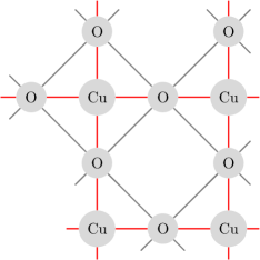
Figure 1: Two dimensional $\rm CuO_{2}$ cubic lattice

We are mainly interested in the interaction between Bloch electrons and lattice phonons. Starting with the standard many-body Hamiltonian, the renormalization flow of Wegner W1 ; W2 yields an effective electron model where the electron-phonon interaction is replaced by an effective electron-electron interaction mediated by the phonons. The leading-order effective Hamiltonian has the general form

$$H_{\text{el}} =\sum_{\mathbf{k},n,\sigma}\epsilon_{n}(\mathbf{k})c_{n\mathbf{k}\sigma}^{\dagger}c_{n\mathbf{k}\sigma}$$

$$+\sum_{\begin{subarray}{c}\mathbf{k}n\sigma,\mathbf{k^{\prime}}m\sigma^{\prime}\\ \mathbf{q}n^{\prime}m^{\prime}\mathbf{GG^{\prime}}\end{subarray}}V^{nn^{\prime}mm^{\prime}}_{\sigma\sigma^{\prime}}(\mathbf{k},\mathbf{k^{\prime}},\mathbf{G},\mathbf{G^{\prime}},\mathbf{q})\;$$

$$\qquad\qquad\cdot c_{n^{\prime}\mathbf{k}+\mathbf{q}+\mathbf{G}\sigma}^{\dagger}c_{m^{\prime}\mathbf{k^{\prime}}-\mathbf{q}+\mathbf{G^{\prime}}\sigma^{\prime}}^{\dagger}c_{m\mathbf{k^{\prime}}\sigma^{\prime}}c_{n\mathbf{k}\sigma},$$ (3)

where $\epsilon(\mathbf{k})$ is the electronic dispersion relation, $\sigma,\sigma^{\prime}$ the electronic spins and $V$ the effective attractive interaction between electrons with momenta $\mathbf{k},\mathbf{k}^{\prime}$ through a phonon with momentum $\mathbf{q}$ and Umklapp vectors $\mathbf{G},\mathbf{G}^{\prime}$. It is worth noting that the Wegner flow method has been previously used to study electron-phonon interactions in other models, see e.g. ACGL .
We are interested in possible pairing mechanism of electrons with momenta $\mathbf{k},\mathbf{k^{\prime}}$, with $\frac{\left|\mathbf{k}-\mathbf{k}^{\prime}\right|}{\left|\mathbf{k}_{F}\right|}\ll 1$ and both momenta are close to the Fermi surface with an effective interaction mediated by phonons with low momenta $\mathbf{q}$. However, in order to obtain an explicitly solvable model, we further simplify this model by concentrating on pairs with equal momenta. Thereby (3) can be restricted to $\mathbf{k}=\mathbf{k}^{\prime}$, and $\mathbf{k}+\mathbf{q}+\mathbf{G}=\mathbf{k^{\prime}}-\mathbf{q}+\mathbf{G^{\prime}}$. Solving for the phonon momentum gives $\mathbf{q}=\frac{\mathbf{G}^{\prime}-\mathbf{G}}{2}$. In the first Brillouin zone (FBZ) this has the trivial solution $\bf q=0$ and four further distinct solutions on the boundary, $\mathbf{q}=(\pi,0)$, $(0,\pi)$, and $(\pi,\pm\pi)$, where the lattice constant $a=1$ in natural units.

Since we are interested in small momentum transfers, we focus on the case of $\bf q=0$. It cannot be overemphasized that this should be considered as an approximation that captures the essential physical mechanism, whereas in an actual physical system any sufficiently small momentum transfer $\bf q$, and likewise any Bloch momentum pairs $\mathbf{k},\mathbf{k^{\prime}}$ that are sufficiently close to each other on the scale of the Fermi momentum $\mathbf{k}_{F}$, i.e. $\frac{\left|\mathbf{k}-\mathbf{k}^{\prime}\right|}{\left|\mathbf{k}_{F}\right|}\ll 1$, can contribute. In Sections V and VI, we study more general pairings and potentials by means of the linearized gap equations. There we provide some arguments and numerical evidence confirming the validity of the approximations $\mathbf{k}=\mathbf{k}^{\prime}$ and $\mathbf{q}=0$ in a simplified exemplary model.

Neglecting electron-electron Coulomb interactions, we obtain a reduced effective Hamiltonian of the form

$$H_{\text{eff}} =\sum_{\mathbf{k}\sigma}\epsilon(\mathbf{k})c_{\mathbf{k}\sigma}^{\dagger}c_{\mathbf{k}\sigma}+\sum_{\begin{subarray}{c}\mathbf{k},\sigma,\sigma^{\prime}\end{subarray}}V(\mathbf{k})\;c_{\mathbf{k}\sigma}^{\dagger}c_{\mathbf{k}\sigma^{\prime}}^{\dagger}c_{\mathbf{k}\sigma^{\prime}}c_{\mathbf{k}\sigma}.$$ (4)

In the following sections, we explore the possible pair formation within this toy model. In the Appendix we briefly outline the standard derivation of the effective electron-electron interaction (3) in the rigid-ion approximation. There one obtains for (4) that

$$V(\mathbf{k}) =-\sum_{\lambda}\frac{1}{\omega_{\lambda}(\mathbf{0})}\left|D_{\lambda}(\mathbf{k})\right|^{2}.$$ (5)

where $\omega_{\lambda}(\mathbf{0})$ is the optical phonon energy at zero momentum, and the electron-phonon coupling $D_{\lambda}(\mathbf{k})$ is given by

$$D_{\lambda}(\mathbf{k})=\mathrm{i}\sqrt{\frac{\hbar N_{\text{cell}}^{3}}{2\omega_{\lambda}(0)\Omega^{4}}}\sum_{\tau}\sum_{\tilde{\mathbf{G}}\in\text{RL}} \mathbf{e}_{\lambda,\tau}(\mathbf{0})\cdot\tilde{\mathbf{G}}\;\frac{\hat{v}_{\text{ei}}^{\tau}(\tilde{\mathbf{G}})}{\sqrt{M_{\tau}}}$$

$$\cdot\int_{\text{cell}}{\mathrm{d}}^{2}r\,\mathrm{e}^{\mathrm{i}\tilde{\mathbf{G}}\cdot\mathbf{r}}\left|u_{\mathbf{k}}(\mathbf{r})\right|^{2},$$ (6)

Here $N_{\text{cell}}$ is the number of primitive cells in a lattice of volume $\Omega$, $\tau$ runs over the atomic basis, $M_{\tau}$ the mass of the $\tau$ ion and $\hat{v}_{\text{ei}}^{\tau}$ the Fourier transform of the spin-independent electron-ion potential, defined as

$$\hat{v}^{\tau}_{\rm ei}({\bf Q})=\int_{\Omega}{\mathrm{d}}^{2}r\,v^{\tau}_{\rm ei}({\bf r})\mathrm{e}^{-\mathrm{i}{\bf Q}\cdot{\bf r}}$$ (7)

Moreover, $e_{\lambda,\tau}$ are the polarization vectors, while $u_{k}$ are the lattice periodic electronic wave functions and the integral is over the volume of the unit cell.

It is worth noting that one obtains a similar expression for the effective electron-electron interaction between pairs $(\mathbf{k},-\mathbf{k})$ when $\mathbf{q}=0$. See the Appendix for details.

II BCS approach to equal momentum pairing

We would like to emphasize that, as pointed out in HL , any pairing, $\mathbf{k},\mathbf{k}^{\prime}$ with $\epsilon(\mathbf{k})=\epsilon(\mathbf{k}^{\prime})$, can lead to the instability of the Fermi sea. Choosing equal momentum pairing allows us to obtain a gap equation that depends on only one momentum. Let us now apply the usual BCS mean-field approach to (4), with the gap function for equal momentum pairing defined by

$$\Delta(\mathbf{k})=V(\mathbf{k})\langle c_{\mathbf{k}\downarrow}c_{\mathbf{k}\uparrow}\rangle.$$ (8)

Following standard arguments we obtain the gap equation

$$\Big{(}\frac{E_{\Delta}(\mathbf{k})}{\tanh\big{(}\frac{E_{\Delta}(\mathbf{k})}{2T}\big{)}}+\frac{V(\mathbf{k})}{2}\Big{)}\Delta(\mathbf{k})=0,$$ (9)

with

$$E_{\Delta}(\mathbf{k})=\sqrt{(\epsilon(\mathbf{k})-\epsilon(\mathbf{k}_{\rm F}))^{2}+|\Delta(\mathbf{k})|^{2}}.$$ (10)

The corresponding equation for the critical temperature $T^{*}$,

$$\frac{E_{0}(\mathbf{k}_{\rm F})}{\tanh\big{(}\frac{E_{0}(\mathbf{k}_{\rm F})}{2T^{*}}\big{)}}=-\frac{V(\mathbf{k}_{\rm F})}{2},$$ (11)

reduces to the particularly simple relation

$$T^{*}=-\frac{V(\mathbf{k}_{\rm F})}{4}.$$ (12)

The linear dependence on the coupling distinguishes this type of pairing from conventional superconductors. Here, the critical pairing temperature $T^{*}$ is directly determined by the strength of the lattice deformation. A particular weakness of our approach is the loss of phase dependence, since the solution of (9) is determined only up to an arbitrary phase function $e^{i\theta(\mathbf{k})}$.

It should be mentioned that in recent years the mathematical properties of conventional BCS theory have been intensively studied HHSS ; FHNS ; FHSS ; HS1 ; HS2 ; FHaiLa ; DeHaiSch with sometimes rather surprising insights FHSchS ; HSey .

III A tight binding model with Jahn-teller type distortion

As an illustrative example, we now augment the ${\rm Cu}{\rm O}_{2}$-model from section I by a Jahn-Teller type distortion. In particular, we will show how such distortions give rise to attractive ${\bf kk}$ interactions sufficient for the occurrence of BCS states with such pairings. Our example of a lattice distortion is again intended to be a simplification of the possible dynamically induced and thus usually localized distortions. Consequently many choices below will also be made with simplicity and transparency of the resulting model in mind.

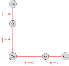
Figure 2: An example of a Jahn-Teller type distortion to ${\rm Cu}{\rm O}_{2}$. On the left, a unit cell with displacements $\delta_{x/y}$ from the positions of the oxygen atoms at the symmetry points $(a/2,0)$ and $(0,a/2)$ along the respective axes is shown.

We begin by statically distorting the two oxygens of each unit cell away from their symmetric equilibrium positions to $r_{{\rm O}^{(1)}}=(a/2+\delta_{x},\,0)$ and $r_{{\rm O}^{(2)}}=(0,\,a/2+\delta_{y})$. Here we adopt dimensionless units with lattice spacing $a=1$. The distortion length parameters $\delta_{x}=\delta_{y}=:\delta$ are taken to be equal and small compared to the lattice constant $a$. This geometry is shown in Figures 2, 3.

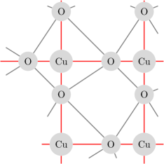
Figure 3: The deformed lattice and bond structure resulting from the distortion of Figure 2.

Next we calculate the electron-phonon coupling $D_{\lambda}(\mathbf{k})$ using a tight-binding wave function

$$\psi_{n,\mathbf{k}}(\mathbf{r})=\frac{1}{\sqrt{N}}\sum_{j,\tau}c_{\tau,\mathbf{k}}^{n}\mathrm{e}^{\mathrm{i}\mathbf{k}\cdot\mathbf{R}_{j}}w_{\tau}(\mathbf{r}-\mathbf{R}_{j\tau}),$$ (13)

where $N=3N_{\text{cell}}$ denotes the number of lattice ions. The coefficients $c_{\tau,\mathbf{k}}^{n}$ are the $n$-th eigenvector of a hopping Hamiltonian in the atomic basis

$${\mathcal{H}}=\begin{pmatrix}\varepsilon_{\rm Cu}&a_{x}&a_{y}\\ a_{x}^{*}&\varepsilon_{{\rm O}_{x}}&c\\ a_{y}^{*}&c^{*}&\varepsilon_{{\rm O}_{y}}\\ \end{pmatrix}$$ (14)

modeled after the lattice structure from Figure 1, with $a_{x}:=t_{1}+t_{1}\mathrm{e}^{-\mathrm{i}k_{x}}$, $a_{y}:=t_{1}+t_{1}\mathrm{e}^{-\mathrm{i}k_{y}}$ and $c:=t_{2}+t_{2}\mathrm{e}^{\mathrm{i}k_{x}}+t_{2}\mathrm{e}^{-\mathrm{i}k_{y}}+t_{2}\mathrm{e}^{\mathrm{i}k_{x}-\mathrm{i}k_{y}}$. The parameter $t_{1}$ corresponds to horizontal and vertical ${\rm Cu}$-${\rm O}$ hopping, while $t_{2}$ is the amplitude for diagonal ${\rm O}$-${\rm O}$ hopping.

Typical values in $t_{1}$-units are $\varepsilon_{\rm Cu}-\varepsilon_{\rm O}\approx 2.5\text{ to }3.5\,t_{1}$, while $t_{2}\approx 0.5\text{ to }0.6\,t_{1}$, with $t_{1}\approx 1.2\text{ to }1.5\,{\rm eV}$ PF ; WMM . Here we take $t_{1}=1.5\,{\rm eV},t_{2}=0.6\,t_{1}$, $\varepsilon_{\rm Cu}=4.5\,{\rm eV}$, while setting the oxygen ground state energy $\varepsilon_{\rm O}$ to zero by a redefinition of the Fermi energy. The resulting dispersion relation has three branches and is shown in Figure 4.

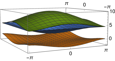
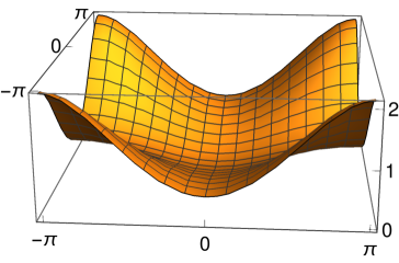
Figure 4: Dispersion relation in the tight-binding model with  $t_{1}=1.5~{}{\rm eV}$, $t_{2}=0.825~{}{\rm eV}$. For the BCS model we consider only the lowest branch (bottom).

For the atomic wave functions we take Gaussians $w_{\tau}(\mathbf{r}):={\mathcal{N}}_{\rho}\mathrm{e}^{-\mathbf{r}^{2}/(4\rho^{2})}$, with width $\rho$ independent of the atomic species $\tau$ and normalization ${\mathcal{N}}_{\rho}^{-1}=\sqrt{2\pi\rho^{2}}$. With this setup the resulting lattice-periodic wave functions are

$$u_{n,\mathbf{k}}(\mathbf{r})={(2\pi)^{2}}\sum_{\tau}c_{\tau,\mathbf{k}}^{n}\sum_{\mathbf{G}\in\text{RL}}\mathrm{e}^{-\mathrm{i}\mathbf{r}\cdot\mathbf{G}}\hat{w}(\mathbf{k}-\mathbf{G})\mathrm{e}^{-\mathrm{i}\mathbf{R}_{\tau}\cdot(\mathbf{k}-\mathbf{G})}$$ (15)

where the integral from the Fourier representation $w(\mathbf{r}):=\int{\rm d}^{2}q\;\mathrm{e}^{\mathrm{i}\mathbf{r}\cdot\mathbf{q}}\hat{w}(\mathbf{q})$ of the atomic wave functions has already been carried out in combination with the lattice summation over $j$. The reciprocal lattice (RL) sum can be performed numerically with an appropriate truncation or analytically using special functions.

Proceeding to the electron-phonon and induced electron-electron interactions (I), we consider here only the leading contributions from the smallest non-zero reciprocal lattice components ${\mathbf{\tilde{G}}}=(\pm 2\pi,0)$, $(0,\pm 2\pi)$. For simplicity we will assume that electron-ion potential to be equal at these momenta and independent of $\tau$. Thus abbreviating $v:=\hat{v}_{\text{ei}}^{\tau}(\pm 2\pi,0)$ we obtain

$$D_{\lambda}(\mathbf{k}) \approx 2\mathrm{i}v\sqrt{\frac{\hbar N_{\text{cell}}^{3}}{2\omega_{\lambda}(\mathbf{0})\Omega^{4}}}\left(\sum_{\tau}\frac{\mathbf{e}_{\lambda,\tau}(\mathbf{0})}{\sqrt{M_{\tau}}}\right)\cdot\begin{pmatrix}2\pi I_{\mathbf{k}}^{a}(2\pi,0)\\ 2\pi I_{\mathbf{k}}^{a}(0,2\pi)\end{pmatrix}$$

$$=\mathrm{i}v\sqrt{\frac{8\pi^{2}\hbar}{\omega_{\lambda}(\mathbf{0})\,\Omega}}\;\mathbf{P}_{\lambda}\cdot\begin{pmatrix}I_{\mathbf{k}}^{a}(2\pi,0)\\ I_{\mathbf{k}}^{a}(0,2\pi)\end{pmatrix},$$ (16)

cancelling $\Omega=a^{2}N_{\text{cell}}$ and recalling that we use natural units with $a=1$. In the second equality we prepare for carrying out the mode sum over $\lambda$ in the effective electron-electron interaction (5) by introducing the polarization sum $\mathbf{P}_{\lambda}:=\sum_{\tau}M_{\tau}^{-1/2}{\mathbf{e}}_{\lambda,\tau}(\mathbf{0})$. Further note that the first equality we already replaced the reciprocal lattice sum over the electronic integral from (I) restricted to ${\mathbf{\tilde{G}}}=(\pm 2\pi,0)$, $(0,\pm 2\pi)$ by twice the anti-symmetric part

$$I_{\mathbf{k}}^{a}(\tilde{\mathbf{G}})=\mathrm{i}\int_{\text{cell}}{\mathrm{d}}^{2}r\,\sin(\tilde{\mathbf{G}}\cdot\mathbf{r})\left|u_{n,\mathbf{k}}(\mathbf{r})\right|^{2}$$ (17)

with ${\mathbf{\tilde{G}}}=(2\pi,0)$, $(0,2\pi)$, as explained in more detail at the end of the appendix.

Guided by (5) we consider the two optical phonon modes with lowest energy. We denote their degenerate zero-momentum energy by $\omega_{0}:=\omega_{\lambda}(\mathbf{0})$. The above mode and atomic sum turns out to be independent of the choice of basis of the doubly degenerate polarization space. Further, using standard methods Sol to analyze the phononic structure of the present model, a basis of polarizations can be chosen with non-zero components purely in the $x$- or $y$-coordinate direction, respectively, yielding polarization sums $\mathbf{P}_{\lambda}=(p,0)$ or $(0,p)$ for the respective phonon modes $\lambda$ for some constant $p\not=0$.

Note that an additional factor proportional to the volume $\Omega$ arises from our interpretation of ${\mathbf{k}}{\mathbf{k}}$ as an effective pairing. In particular, we consider $V(\mathbf{k})$ as an approximation of the interaction between electrons with small relative momenta. Hence, the sums in (3) run over momenta in a small neighborhood of $\mathbf{k}$. Overall this yields a factor proportional to the number of states in this neighborhood, which in turn is proportional to the volume $\Omega$.

Any overall scale factors arising here are understood to be absorbed into the effective interaction constant $v$.

Altogether this yields a contribution to the effective electron-electron potential of

$$V(\mathbf{k})\approx-\frac{8\pi^{2}\hbar|pv|^{2}}{\omega_{0}^{2}}\left(\left|I_{\mathbf{k}}^{a}(2\pi,0)\right|^{2}+\left|I_{\mathbf{k}}^{a}(0,2\pi)\right|^{2}\right).$$ (18)

IV Results for the Gap $\Delta$ and Pair-Wave Densities

We can now numerically demonstrate that the simplified distortion scheme from Figure 2 leads to a non-vanishing equal-momentum potential $V(\mathbf{k})$. In Figure 5 the result for distortion parameter $\delta=0.05a$ is shown, with the remaining model parameters as in Section III. The atomic wave function width $\rho=0.05a$ is chosen rather small for simplicity, as for larger widths overlaps of neighboring atomic wave functions are longer negligible if we require that (15) are well normalized. The numerics also confirm that $V(\mathbf{k})$ vanishes in the symmetric case with displacement $\delta=0$, whereas $V<0$ inside the first Brillouin zone if distortions are present.

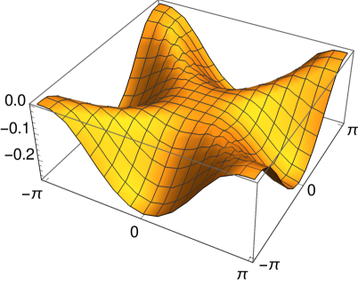
Figure 5: The effective electron-electron potential $V$ for the lowest electron branch in the first Brillouin zone, shown in units of $\hbar|pv|^{2}/\omega_{0}^{2}$ for distortion parameter $\delta=\rho=0.05a$.

Applying the results described in Section II, we obtain BCS states formed by $\mathbf{k}\mathbf{k}$ pairs for temperatures $T$ below the critical temperature $T^{*}$. For this purpose we use the dispersion relation obtained as the lowest eigenvalue of the hopping Hamiltonian (14). The gap function $\Delta(\mathbf{k})$ can then be obtained directly from (9). For $T<T^{*}$ a non-vanishing gap starts to develop in the vicinity of the maxima of $V$ on the Fermi surface and extends to a neighborhood of the full Fermi surface when lowering the temperature further as shown in Figure 6.

It should be recalled here that (9) yields only the absolute value $|\Delta(\mathbf{k})|$ of the gap function. On the other hand, the phase of the order parameter is not fixed by the present method, even to the extent that any choice of phase is consistent with this gap equation. The pair density in position space evaluated in the BCS state $\Gamma$ from Section II is given by

$$\langle\psi_{\uparrow}(\mathbf{r})\psi_{\downarrow}(\mathbf{r})\rangle_{\Gamma}=\int_{\text{FBZ}}{\mathrm{d}}^{2}k\,\alpha(\mathbf{k})\cos(2\mathbf{k}\cdot\mathbf{r})(u_{\mathbf{k}}(\mathbf{r}))^{2},$$ (19)

where by definition the Bloch field in the tight-binding model is $\psi_{\sigma}(\mathbf{r})=\int{\mathrm{d}}^{2}k\,\mathrm{e}^{\mathrm{i}\mathbf{k}\cdot\mathbf{r}}u_{\mathbf{k}}(\mathbf{r})c_{\mathbf{k}\sigma}$, we used the even parity symmetry of $\alpha$ and $u$ under $\mathbf{k}\leftrightarrow-\mathbf{k}$ and we note that $u_{\mathbf{k}}$ is real-valued. In Figures 7 and 8 we show some results for two natural choices of the phase of the pairing order $\alpha(\mathbf{k})=\langle c_{\mathbf{k}\downarrow}c_{\mathbf{k}\uparrow}\rangle$. In both cases, clear spatial modulations of the pair density provide evidence for the emergence of pair density waves (PDW) in the present model.

$T\approx\ 0.9T^{*}$

$T\approx 0.75T^{*}$

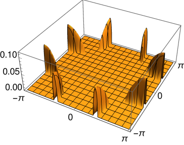
$T\approx 0.5T^{*}$

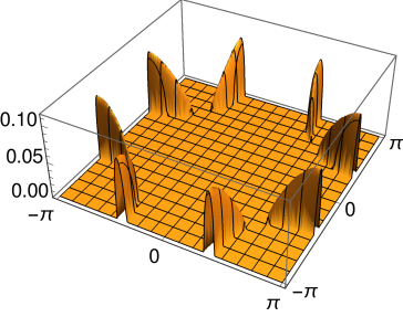
$T\approx 0.4T^{*}$

Figure 6: Absolute value of the Gap function $\Delta$ in a tight-binding model with parameters $\rho=0.05a$, $\delta=0.05a$, $t_{1}=1.5~{}{\rm eV}$, $t_{2}=0.8~{}{\rm eV}$. The Fermi surface with $\mu=0.8~{}{\rm eV}$ is indicated in red on the first gap plot.

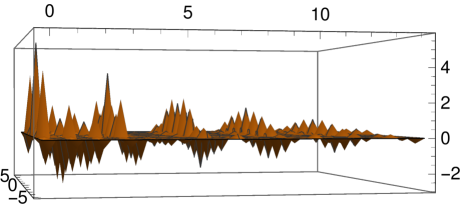
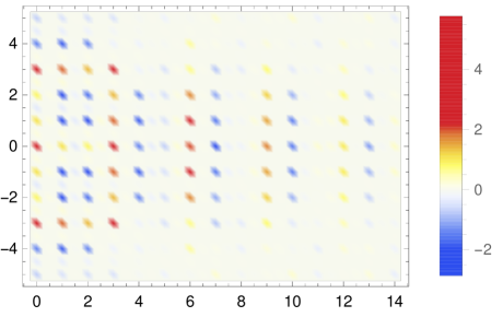
Figure 7: Pair-wave density (19) in configuration space for order parameter $\alpha(\mathbf{k})=|\alpha(\mathbf{k})|$ from Figure 6 at $T\approx\ 0.9T^{*}$, calculated via Riemann sums with $N=101$ support points in both coordinate directions.

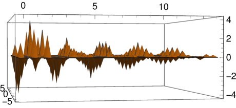
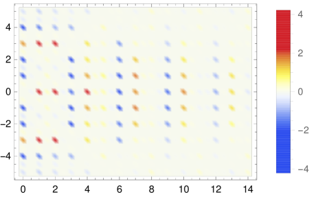
Figure 8: Pair-wave density (19) with additional d-wave-like phase $\alpha(\mathbf{k})=\sigma(\mathbf{k})|\alpha(\mathbf{k})|$ at $T\approx\ 0.9T^{*}$, $\sigma(\mathbf{k}):=\operatorname{sgn}(k_{x}^{2}-k_{y}^{2})$.

Finally let us note that our model can easily be refined concerning various aspects. For example, one could take into account the influence of the distortion on the hopping parameters $t_{1(2)}$ or include contributions of higher-order reciprocal lattice components $\mathbf{\tilde{G}}$ in (III). Pursuing here would take us well beyond our present focus on the salient features of the proposed pairing mechanism. We hope that such questions will be explored in subsequent works.

V Distinguished roles of $\mathbf{k},\mathbf{k}$ and $\mathbf{k},-\mathbf{k}$ among fully general pairings in the linearized gap equation

The linearized problem allows a direct comparison of the standard Cooper pairing $(\mathbf{k},-\mathbf{k})$ with the fully generalized pairing $(\mathbf{k},\mathbf{k}^{\prime})$. We begin by following the same steps and approximations as in Section III to obtain the electron-phonon potential for general pairs $(\mathbf{k},\mathbf{k}^{\prime})$ with momentum transfer $\mathbf{q}=0$ as

$$V(\mathbf{k},\mathbf{k}^{\prime})\approx-\frac{8\pi^{2}\hbar|pv|^{2}}{\omega_{0}^{2}}\begin{pmatrix}I_{\mathbf{k}}^{a}(2\pi,0)\\ I_{\mathbf{k}}^{a}(0,2\pi)\end{pmatrix}\cdot\begin{pmatrix}I_{\mathbf{k}^{\prime}}^{a}(2\pi,0)\\ I_{\mathbf{k}^{\prime}}^{a}(0,2\pi)\end{pmatrix},$$ (20)

with reduced effective Hamiltonian

$$H_{\text{eff}} =\sum_{\mathbf{k}\sigma}\epsilon(\mathbf{k})c_{\mathbf{k}\sigma}^{\dagger}c_{\mathbf{k}\sigma}+\!\!\!\sum_{\begin{subarray}{c}\mathbf{k}\sigma\mathbf{k^{\prime}}\sigma^{\prime}\end{subarray}}V(\mathbf{k},\mathbf{k^{\prime}})\;c_{\mathbf{k}\sigma}^{\dagger}c_{\mathbf{k^{\prime}}\sigma^{\prime}}^{\dagger}c_{\mathbf{k^{\prime}}\sigma^{\prime}}c_{\mathbf{k}\sigma}.$$ (21)

We note that this is consistent with (4), where the latter is obtained by further reduction to quasi-free states supported on $(\mathbf{k},\mathbf{k})$ pairs only. The potential has the general form

$$-V(\mathbf{k},\mathbf{k}^{\prime})=D_{1}(\mathbf{k})D_{1}(\mathbf{k}^{\prime})+D_{2}(\mathbf{k})D_{2}(\mathbf{k}^{\prime}),$$ (22)

where $D_{2}(k_{y},k_{x})=D_{1}(k_{x},k_{y})=:D(\mathbf{k})$ for the presently studied model.

The linearized gap equation reads

$$\Delta=-\frac{1}{2}L_{\beta}V\Delta$$ (23)

with 2-body operator

$$L_{\beta}(\mathbf{k},\mathbf{k}^{\prime})=\frac{\tanh(\frac{\beta}{2}\epsilon_{\mu}(\mathbf{k}))+\tanh(\frac{\beta}{2}\epsilon_{\mu}(\mathbf{k}^{\prime}))}{\epsilon_{\mu}(\mathbf{k})+\epsilon_{\mu}(\mathbf{k}^{\prime})}$$ (24)

and we abbreviate $\epsilon_{\mu}(\mathbf{k}):=\epsilon(\mathbf{k})-\mu$. Here we use the notation of (HL, , Appendix A), where the reader can also find a succinct derivation and further explanations.

For the toy model at hand, the product operator in (23) is a multiplication operator and hence the eigenvalue problem becomes trivially solvable. The critical $\beta^{*}=1/T^{*}$ is defined by the emergence of a non-trivial solution $(\mathbf{k},\mathbf{k}^{\prime})$ of

$$-\frac{1}{2}L_{\beta^{*}}(\mathbf{k},\mathbf{k}^{\prime})V(\mathbf{k},\mathbf{k}^{\prime})=1$$ (25)

and $-\frac{1}{2}L_{\beta}V<1$ for all $\beta<\beta^{*}$.

For simplicity, let us now adopt the perspective of fixing a temperature $T^{*}$ and then slowly turning on the potential (e.g. by a coupling constant). From this perspective the global maxima of the operator kernel from (25) give the emerging dominant pairings. For the parameters from Section IV, the numerics yield exactly the conventional BCS pairings $(\mathbf{k},-\mathbf{k})$ and the alternative pairings $(\mathbf{k},\mathbf{k})$ studied in the present paper, as seen in Figures 9, 10.

One arrives at a similar conclusion by qualitative considerations: when the kinetic kernel $L_{\beta}$ provides the dominant scale, as for the present model parameters, the first pairs to emerge are approximately located at the maximum of the potential $V$, when both momenta are on the Fermi surface $\epsilon_{\mu}(\mathbf{k})=0=\epsilon_{\mu}(\mathbf{k}^{\prime})$ (see HL ). In our model, the maxima of the potential $V(\mathbf{k},\mathbf{k}^{\prime})$ on the Fermi surface are located at points exactly of the form $\mathbf{k}^{\prime}=\pm\mathbf{k}$. Thereby, close to $T^{*}$, other types of pairing are excluded in our model. This further motivates the study of the $(\mathbf{k},\mathbf{k})$ pairing on the level of the fully non-linear gap equation in Section IV and confirms the necessity of considering alternative pairings.

Finally, these two distinguished types of pairing can be compared analytically in the present model: It is easily seen that $V(\mathbf{k},\mathbf{k})=V(\mathbf{k},-\mathbf{k})$ for all $\mathbf{k}\in\text{FBZ}$. Similarly $\epsilon_{\mu}(\mathbf{k})=\epsilon_{\mu}(-\mathbf{k})$ implies $L_{\beta}(\mathbf{k},-\mathbf{k})=L_{\beta}(\mathbf{k},\mathbf{k})$. Hence these two pairings correspond to exactly the same eigenvalue at the level of the linearized gap equation (23). Thus they appear also at exactly the same critical temperature. Numerically this can be visualized by plotting $M(\mathbf{k}):=\max_{k^{\prime}\in\text{FBZ}}(-L_{\beta^{*}}(\mathbf{k},\mathbf{k}^{\prime})V(\mathbf{k},\mathbf{k}^{\prime}))$, as shown in Figure 9, and subsequently plotting $-(L_{\beta^{*}}V)(\mathbf{k}_{\text{max}},\mathbf{k}^{\prime})$ at one of the global maxima $\mathbf{k}_{\text{max}}$ of $M$, as shown in Figure 10. In the subsequent Section VI we will argue that this parity between $(\mathbf{k},\mathbf{k})$ and $(\mathbf{k},-\mathbf{k})$ is not a true symmetry of nature. Namely, we will demonstrate that the assumption $\mathbf{q}=0$ can be justified for $(\mathbf{k},\mathbf{k})$ but fails for the conventional pairing, when also interactions with non-vanishing momentum transfer are included.

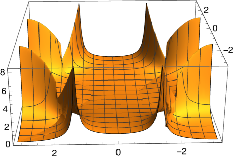
Figure 9: The kernel maximum function $M(\mathbf{k}):=\max_{k^{\prime}\in\text{FBZ}}(-L_{\beta^{*}}(\mathbf{k},\mathbf{k}^{\prime})V(\mathbf{k},\mathbf{k}^{\prime}))$ from the linear gap equation at $\mu=0.85~{}\text{eV}$, where $\beta^{*}=100~{}\text{eV}^{-1}$.

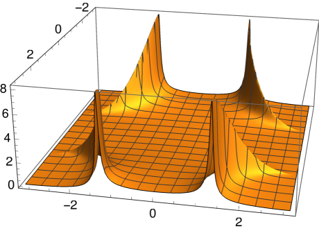
Figure 10: The plot of the linear gap kernel $-(LV)(\mathbf{k}_{\text{max}},\mathbf{k}^{\prime})$ as a function of $\mathbf{k}^{\prime}$ at one of the global maxima $\mathbf{k}_{\text{max}}$ of $M$ shows that exactly the two pairings $(\mathbf{k}_{\text{max}},\mathbf{k}_{\text{max}})$ and $(\mathbf{k}_{\text{max}},-\mathbf{k}_{\text{max}})$ emerge at the critical temperature. All other parameters are as in Figure 9.

VI Emergence of equal momentum pairings for interactions with small momentum transfer.

Let us now consider the question of the stability of the observed $(\mathbf{k},\mathbf{k})$-pairings when interactions with non-vanishing momentum transfers are included in the model. For this we return to the full Wegner interaction

$$H_{\text{int}}=\sum_{\begin{subarray}{c}\mathbf{k}\sigma\mathbf{k^{\prime}}\sigma^{\prime}\mathbf{q}\end{subarray}}V_{\sigma\sigma^{\prime}}(\mathbf{k},\mathbf{k^{\prime}},\mathbf{q})\;c_{n^{\prime}\mathbf{k}+\mathbf{q}\sigma}^{\dagger}c_{m^{\prime}\mathbf{k^{\prime}}-\mathbf{q}\sigma^{\prime}}^{\dagger}c_{m\mathbf{k^{\prime}}\sigma^{\prime}}c_{n\mathbf{k}\sigma},$$

where Umklapp momenta are suppressed for notational simplicity. As we are only interested in small $\mathbf{q}$ and to remain comparable to our main results, we will not amend our model to include a full phononic sector and instead assume that the electron-phonon interaction is well approximated by $D_{\lambda}(\mathbf{k},\mathbf{q})\approx D_{\lambda}(\mathbf{k})$ for small $\mathbf{q}$ and taken to vanish otherwise. To obtain a self-adjoint interaction we use an appropriate extension of electron-phonon part from (Appendix A: Electron-Phonon Coupling in ${\rm\mathbb{CuO_{2}}}$) to nonzero $\mathbf{q}$ given by

$$W(\mathbf{k},\mathbf{k}^{\prime},\mathbf{q}) :=\frac{1}{2}\sum_{\lambda}\left(D_{\lambda}(\mathbf{k}^{\prime})D_{\lambda}(\mathbf{k})\right.$$

$$\qquad\qquad\qquad\left.+D_{\lambda}(\mathbf{k}^{\prime}-\mathbf{q})D_{\lambda}(\mathbf{k}+\mathbf{q})\right).$$ (26)

Here we already used the approximation that $\omega_{\lambda}(\mathbf{q})\approx\omega_{0}\not=0$, constant and independent of the optical phonon mode $\lambda$. Hence the kinetic part from the Wegner interaction (Appendix A: Electron-Phonon Coupling in ${\rm\mathbb{CuO_{2}}}$) becomes independent of the phonon mode and the mode sum can be performed as above. On the other hand the matrix element of $H_{\text{int}}$ providing the kernel for the numerical study described below now has to be symmetrized under simultaneously exchanging $\mathbf{k}\leftrightarrow\mathbf{k}^{\prime}$ and $\mathbf{q}\leftrightarrow-\mathbf{q}$ in order to conform to Fermi statistics, which yields

$$V(\mathbf{k},\mathbf{k}^{\prime},\mathbf{q})=-\frac{4\omega_{0}(dd^{\prime}+\omega_{0}^{2})}{(d^{2}-d^{\prime 2})^{2}+4(dd^{\prime}+\omega_{0}^{2})^{2}}W(\mathbf{k},\mathbf{k}^{\prime},\mathbf{q}),$$ (27)

where $d=\epsilon(\mathbf{k}+\mathbf{q})-\epsilon(\mathbf{k})$ and $d^{\prime}=\epsilon(\mathbf{k}^{\prime}-\mathbf{q})-\epsilon(\mathbf{k}^{\prime})$.

We now study the spectrum of the operator $-\frac{1}{2}VL_{\beta}$ from the linearized gap equation (23) using a suitable discretization. As the linearized approximation of the gap equation is usually expected to be valid close to $T^{*}$, the results from the main part of our paper suggest that the $\mathbf{k}\mathbf{k}$-pairing instability in the present model should appear close to the boundary of the first Brillouin zone. For this reason we use a discretization with periodic boundary conditions. To not accidentally suppress either the $(\mathbf{k},-\mathbf{k})$ or the expected novel $(\mathbf{k},\mathbf{k})$-pairings, we further carefully choose the discretization lattice to include both the origin and the boundary points of the form $(k_{x},\pi)$ and $(\pi,k_{y})$. For the numerical implementation we observe that at the level of the linearized gap equation (23), the various PDW-type pairing orbits $(\mathbf{k},\mathbf{k}^{\prime})=(\mathbf{K}+\mathbf{p},\mathbf{K}-\mathbf{p})$ decouple. As in Section V we identify the dominant pairing mechanism from the largest eigenvalue of $-\frac{1}{2}VL_{\beta}$, which we calculate here as function of $\mathbf{K}$ together with the corresponding eigenfunctions. For suitable parameters the numerical results shown in Figures 11–15 provide further supporting evidence for our model.

Due to the discretization approach the accessible lattice spacings are unfortunately limited by available computational resources. For the present calculation we choose a practical lattice discretizations of the first Brillouin zone with $N_{\text{pt}}=20$ points per coordinate axis. We extend the potential via (26) to a $\mathbf{q}$-radius of $2$ lattice spacings. The lattice spacing limits the ranges of numerically accessible temperatures $T=\beta^{-1}$ and $\omega_{0}$ from below, as the essential features of both the two-body operator $L_{\beta}$ and the Wegner potential have to be resolved with sufficient accuracy. Both become less smooth as the corresponding parameter values are lowered. Due to these numerical limitations we choose here $\beta=50\;\text{eV}^{-1}$ and we lowered $\omega_{0}$ very carefully starting from a physically very large value $\omega_{0}=1\;\text{eV}$. Other model parameters are chosen as in Section III. Slowly lowering the phonon dispersion constant, we see that at larger $\omega_{0}$ that the largest eigenvalues are at $\mathbf{K}=0$, corresponding to conventional $(\mathbf{k},-\mathbf{k})$-pairing, see Figure 11. The corresponding wave function as function of $\mathbf{p}$ has the usual structure and is spread out over a close vicinity of the Fermi surface as seen in Figure 12.

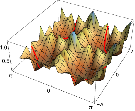
Figure 11: Largest eigenvalue of $-VL_{\beta}$ for $\omega_{0}=0.5\;\text{eV}$ as function of $\mathbf{K}$ (other parameters as described in the text). Here and in the following figures we will indicate the Fermi surface for $\mu=0.85\;\text{eV}$ in red. The boundary points of the discretization will always only be included on the positive sides of the corresponding axes. The plot meshes are from now on matched to the discretization.

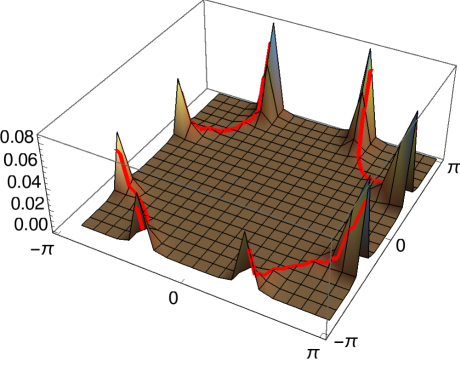
Figure 12: Absolute square of the wave function for $\mathbf{K}=0$ in Figure 11 as function of $\mathbf{p}$.

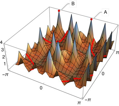
Figure 13: Largest eigenvalue for $\omega_{0}=0.33\;\text{eV}$ as function of $\mathbf{K}$ (other parameters as described in the text). The eigenvalues at “A”, “B” and at other similar peaks are dominating over the eigenvalue at the origin $\mathbf{K}=0$.

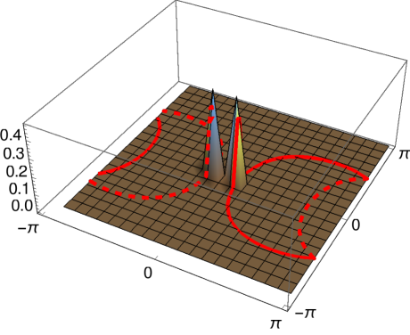
Figure 14: Absolute square of the wave function for $\mathbf{K}=(\frac{3}{10}\pi,\pi)$ (point “A“ in Figure 13) as function of $\mathbf{p}$. Solid and dashed red lines show the Fermi surface for the two electron momenta $\mathbf{K}+\mathbf{p}$ and $\mathbf{K}-\mathbf{p}$, respectively. The energy difference between the two peaks is proportional to $\omega_{0}$.

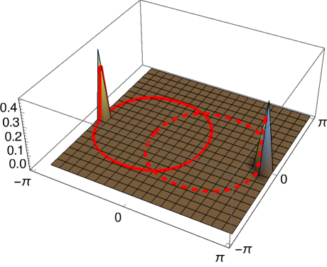
Figure 15: Absolute square of the wave function for $\mathbf{K}=(-\frac{7}{10}\pi,\pi)$ (point “B“ in Figure 13) as function of $\mathbf{p}$, showing that the wave function is concentrated near $(\pm\pi,0)$.

When $\omega_{0}$ is further decreased additional peaks start to form, in particular at the boundary of the first Brillouin zone, as seen in Figure 13 for $\omega_{0}=0.33\;\text{eV}$. Already at this value of $\omega_{0}$ they dominate over the eigenvalue at $\mathbf{K}=0$. An inspection of the corresponding eigenfunctions reveals for the eigenvalue peak labeled “A” in Figure 13 a strongly concentrated wave-function near $\mathbf{p}=0$. Hence this yields $\mathbf{k}\mathbf{k}$-pairings as studied in this paper and thereby provides evidence supporting the approximation of vanishing momentum transfer.

The additional peaks from Figure 13 can be explained by periodic boundary conditions. As an example, the wave function for the eigenvalue peak “B” is shown in Figure 15. Here we can see a strong concentration close to vectors of the halved reciprocal lattice on the boundary of the first Brillouin zone. This eigenvector is however physically equivalent to the eigenvector from point “A”, as can be seen by translating both $\mathbf{K}$ and $\mathbf{p}$ by $(\pi,0)$ and using periodicity. All remaining peaks can be similarly explained in terms of ordinary “A”-type $\mathbf{k}\mathbf{k}$-peaks by invoking the periodic boundary conditions.

Let us note that the electron energy difference between $\mathbf{K}+\mathbf{p}_{1/2}$ at the two peaks $\mathbf{p}_{1/2}$ in Figure 14 is comparable to $\omega_{0}$. Hence can expect for physically small choices of $\omega_{0}$ that the wave function is very well approximated by replacing it with just a single delta peak, which then yields exactly the model studied in the main part of this paper. On the other hand the results from Figures 11 and 12 show that the same approximation is not justified for the ordinary $(\mathbf{k},-\mathbf{k})$ pairing.

We conclude this appendix by giving an explanation to the distinct behaviors of the $(\mathbf{k},\mathbf{k})$ and $(\mathbf{k},-\mathbf{k})$ wave functions. Let us consider the kinetic term in the symmetrized form of the Wegner potential from (27). Now we note that there are configurations of $\mathbf{k}$, $\mathbf{k}^{\prime}$ and $\mathbf{q}$ such that the absolute value of the parameter $\varepsilon:=dd^{\prime}+\omega_{0}^{2}$ becomes small. In the regime $\varepsilon\to 0$ we find the emergence of a Dirac delta potential

$$V(\mathbf{k},\mathbf{k}^{\prime},\mathbf{q})\overset{\varepsilon\to 0}{\longrightarrow}\mp 2\pi\omega_{0}\delta(d^{2}-d^{\prime 2})W$$ (28)

and this interaction is an attractive or repulsive if the sign of $\varepsilon$ is positive or negative, respectively. As the scattering processes most frequently take place close to the Fermi surface, the energy differences $d=\epsilon(\mathbf{k}+\mathbf{q})-\epsilon(\mathbf{k})$ and $d^{\prime}=\epsilon(\mathbf{k}^{\prime}-\mathbf{q})-\epsilon(\mathbf{k}^{\prime})$ tend to be close to zero. Hence the case $\varepsilon\geq 0$ is favoured, yielding a preference of nature for the attractive delta.

However, the mechanism (28) can only contribute to the attractive interaction for $(\mathbf{k},\mathbf{k})$ pairs and not for the conventional $(\mathbf{k},-\mathbf{k})$ pairs, since in the latter case we have $d=d^{\prime}$ and then $\varepsilon\geq\omega_{0}^{2}>0$ prevents the realization of the limit in (28).

Conclusion

We investigate a novel BCS-type pairing mechanism in which electron-electron attraction is mediated by the interaction of low-momentum optical phonons and Jahn-Teller-type lattice distortions. To keep the model as simple as possible and allow for explicit calculations, we focus on the pairing of electrons with equal momenta and give numerical evidence to validate this approximation. To demonstrate how this novel pairing mechanism can lead to instability of the Fermi sea, we consider a particular distortion of a planar ${\rm CuO}_{2}$ lattice and using a tight-binding approximation, we numerically calculate the BCS gap function in this case. In the resulting toy model the Fermi sea is unstable towards equal momentum pairing below a certain critical temperature $T^{*}$. Due to the simplicity of the approach, which also omits Coulomb interactions of electrons as well as density-density interactions and exchange energies, we expect $T^{*}$ to represent not the actual critical temperature describing macroscopic coherence, but the existence of localized pairings such as the pseudogap. It is interesting to note that this appears to be the first microscopic model in which the pair density displays the characteristic features of a pair density wave (PDW).

Appendix A: Electron-Phonon Coupling in ${\rm\mathbb{CuO_{2}}}$

In order to get an expression for the electron-phonon potential, we follow the standard method outlined in many textbooks, e.g. Han ; Sol . However, we take into account the effect of reciprocal lattice vectors and Umklapp processes since they play important part in our discussion of electron pairs with equal momenta.

Let $\Omega$ be the volume of a lattice with $N_{cell}$ primitive cell, $N_{e}$ electrons and let ${\bf r}$ denotes the position of an electron. Using this notation, the electron-ion potential in the rigid ion approximation can be written as

$$V_{\text{el-ion}}=\sum_{l=1}^{N_{\text{e}}}\sum_{j=1}^{N_{\text{cell}}}\sum_{\tau}v^{\tau}_{\text{ei}}({\bf r}_{l}-{\bf R}_{\tau j}),$$ (29)

where ${\bf R}_{\tau j}$ is the position of the “$\tau$” atom in the “jth” primitive cell and $\tau$ runs over the atomic basis. Note that $V_{\text{el-ion}}$ is periodic in the lattice parameter. Our main assumption is that $v^{\tau}_{\text{ei}}$ is spin independent and has a Fourier representation such that

$$v^{\tau}_{\text{ei}}({\bf r})=\dfrac{1}{\Omega}\sum_{{\bf Q}}\hat{v}^{\tau}_{\text{ei}}({\bf Q})\mathrm{e}^{\mathrm{i}{\bf Q\cdot r}},$$ (30)

Note, that this assumption is fulfilled for example if $v^{\tau}_{\text{ei}}$ is periodic in the size of the lattice and bounded.

In second quantization notation, this potential can be written in terms of the creation (annihilation) operator $c^{\dagger}_{n{\bf k}\sigma}(c_{n{\bf k}\sigma})$ of the one-particle electronic states characterized by the Bloch eigenstate $\psi_{n{\bf k}\sigma}$, with band index $n$ , wave number $k$ and spin $\sigma$, as follows

$$V_{\text{el-ion}}=\sum_{j,\tau}\sum_{\begin{subarray}{c}n,m\\ \sigma\\ \bf{k^{\prime},k}\in\text{FBZ}\end{subarray}} \Big{\{}\int_{\Omega}{\mathrm{d}}^{2}r\,\psi_{n{\bf k^{\prime}}\sigma}^{*}({\bf r})v^{\tau}_{\text{ei}}({\bf r}-{\bf R}_{\tau j})\psi_{m{\bf k}\sigma}({\bf r})\Big{\}}$$

$$\cdot c^{\dagger}_{n{\bf k^{\prime}}\sigma}c_{m{\bf k}\sigma}.$$ (31)

Taking into account the displacement of the ions from their equilibrium position, the ionic position can be written as

$${\bf R}_{\tau j}={\bf R}^{0}_{\tau j}+{\bf u}({\bf R}^{0}_{\tau j}),$$ (32)

where ${\bf R}^{0}_{\tau j}$ is the equilibrium position of the $\tau j$ ion, while ${\bf u}_{\tau j}$ its displacement.

Now for small displacements, the potential can be expanded to first order as

$$v^{\tau}_{\text{ei}}({\bf r}-{\bf R}_{\tau j})=v^{\tau}_{\text{ei}}({\bf r}-{\bf R}^{0}_{\tau j})-{\bf\nabla}_{{\bf r}}v^{\tau}_{\text{ei}}({\bf r}-{\bf R}^{0}_{\tau j})\cdot{\bf u}({\bf R}^{0}_{\tau j})+O(u^{2}).$$ (33)

Inserting this expansion in (Appendix A: Electron-Phonon Coupling in ${\rm\mathbb{CuO_{2}}}$), the first term gives the “static” electron-ion interaction while the second is the electron-phonon interaction. Expressing the displacement of ions in terms of the phonon creation and annihilation operators $a^{\dagger}_{\lambda}({\bf q})$, $a_{\lambda}({\bf q})$, where $\lambda$ is the branch index and ${\bf q}$ is the phonon momentum taking values in the first Brillouin zone (FBZ), the electron-phonon interaction takes the form

$$V_{\text{el-ph}}=-\sum_{{\bf q}\in\text{FBZ}} \sum_{\begin{subarray}{c}n,m\\ \lambda,\sigma\end{subarray}}\sum_{{\bf k^{\prime},k}}D^{nm}_{\lambda,\sigma}({\bf k^{\prime},k},{\bf q})$$

$$c^{\dagger}_{n{\bf k^{\prime}}\sigma}c_{m{\bf k}\sigma}\big{(}a_{\lambda}({\bf q})+a^{\dagger}_{\lambda}(-{\bf q})\big{)}.$$ (34)

Where the electron-phonon coupling is given by

$$D^{nm}_{\lambda,\sigma}({\bf k^{\prime},k,q})= \sum_{j,\tau}\sqrt{\dfrac{\hbar}{2M_{\tau}N_{\text{cell}}\omega_{\lambda}({\bf q})}}{\bf e}_{\lambda,\tau}({\bf q})\mathrm{e}^{\mathrm{i}{\bf q}\cdot{\bf R}^{0}_{\tau j}}$$

$$\Big{\{}\int_{\Omega}{\mathrm{d}}^{2}r\,\psi_{n{\bf k^{\prime}}\sigma}^{*}({\bf r}){\bf\nabla}_{{\bf r}}v^{\tau}_{\text{ei}}({\bf r}-{\bf R}^{0}_{\tau j})\psi_{m{\bf k}\sigma}({\bf r})\Big{\}}.$$ (35)

Where ${\bf e}_{\lambda,\tau}({\bf q})$ are the polarization vectors extracted from the eigenvector of the Dynamical matrix corresponding to eigenvalue $\omega_{\lambda}({\bf q})$. Using that $\psi_{m{\bf k}\sigma}$ are Bloch functions and summing over $j$, a simple calculation shows that the electron-phonon potential can be expressed in the terms of vectors in the reciprocal lattice (RL) as

$$V_{\text{el-ph}}=-\sum_{\begin{subarray}{c}n,m,\lambda\\ \sigma\end{subarray}} \sum_{{\bf q},{\bf k}\in\text{FBZ}}\sum_{\begin{subarray}{c}{\bf G}\in\text{RL}\\ {\bf k+q+G}\in\text{FBZ}\end{subarray}}D^{nm}_{\lambda,\sigma}({\bf k},{\bf G},{\bf q})$$

$$\cdot c^{\dagger}_{n{\bf k+q+G}\sigma}c_{m{\bf k}\sigma}\big{(}a_{\lambda}({\bf q})+a^{\dagger}_{\lambda}(-{\bf q})\big{)},$$ (36)

where the coupling is now given by

$$D^{nm}_{\lambda,\sigma}({\bf k},{\bf G},{\bf q})= \sum_{\tau}\sqrt{\dfrac{\hbar N_{\text{cell}}}{2M_{\tau}\omega_{\lambda}({\bf q})}}e^{-\mathrm{i}{\bf G}\cdot{\bf R}^{0}_{\tau}}{\bf e}_{\lambda,\tau}({\bf q})$$

$$\cdot\Big{\{}\int_{\Omega}{\mathrm{d}}^{2}r\,\psi_{n{\bf k+q+G}\sigma}^{*}({\bf r}){\bf\nabla}_{{\bf r}}v^{\tau}_{\rm ei}({\bf r})\psi_{m{\bf k}\sigma}({\bf r})\Big{\}}.$$ (37)

Using the Fourier representation of the electron-ion potential (30) and introducing the lattice periodic functions $u_{m{\bf k}\sigma}$ defined through $\psi_{m{\bf k}\sigma}({\bf r})=\dfrac{1}{\sqrt{\Omega}}\mathrm{e}^{\mathrm{i}{\bf k\cdot r}}u_{m{\bf k}\sigma}$, the coupling now takes the form

$$D^{nm}_{\lambda,\sigma}({\bf k},{\bf G},{\bf q})=\mathrm{i} \sum_{\tau,{\bf Q}}\dfrac{1}{\Omega^{2}}\sqrt{\dfrac{\hbar N_{cell}}{2M_{\tau}\omega_{\lambda}({\bf q})}}\mathrm{e}^{-\mathrm{i}{\bf G}\cdot{\bf R}^{0}_{\tau}}$$

$$\cdot\big{(}{\bf e}_{\lambda,\tau}({\bf q})\cdot{\bf Q}\big{)}\hat{v}^{\tau}_{ei}({\bf Q})$$

$$\cdot\Big{\{}\int_{\Omega}{\mathrm{d}}^{2}r\,\mathrm{e}^{\mathrm{i}{\bf Q}\cdot{\bf r}}\mathrm{e}^{-\mathrm{i}{(\bf q+G})\cdot{\bf r}}u_{n{\bf k+q+G}\sigma}^{*}({\bf r})u_{m{\bf k}\sigma}({\bf r})\Big{\}}.$$ (38)

Finally, since the functions $u_{m{\bf k}\sigma}$ are lattice periodic (with trivial spin dependence), the integral over the volume can be reduced to integrals over the primitive cells. Therefore,

$$D^{nm}_{\lambda,\sigma}({\bf k},{\bf G},{\bf q}) =\mathrm{i}\dfrac{N_{\text{cell}}}{\Omega^{2}}\sum_{\begin{subarray}{c}\tau\\ {\bf\tilde{G}}\in\text{RL}\end{subarray}}\sqrt{\dfrac{\hbar N_{\text{cell}}}{2M_{\tau}\omega_{\lambda}({\bf q})}}\mathrm{e}^{-\mathrm{i}{\bf G}\cdot{\bf R}^{0}_{\tau}}$$

$$\cdot\big{(}{\bf e}_{\lambda,\tau}({\bf q})\cdot{(\bf q+G+\tilde{G}})\big{)}\hat{v}^{\tau}_{ei}({\bf q+G+\tilde{G}})$$

$$\cdot\Big{\{}\int_{\text{cell}}{\mathrm{d}}^{2}r\,\mathrm{e}^{\mathrm{i}{\bf\tilde{G}}\cdot{\bf r}}u_{n{\bf k+q+G}\sigma}^{*}({\bf r})u_{m{\bf k}\sigma}({\bf r})\Big{\}},$$ (39)

where the integral is now over the volume of the primitive cell.

Using the lowest order approximation of the Wegner flow W1 ; W2 , one obtains the following effective electronic Hamiltonian

$$H_{\text{el}} =\sum_{\mathbf{k},n,\sigma}\epsilon_{n}(\mathbf{k})c_{n\mathbf{k}\sigma}^{\dagger}c_{n\mathbf{k}\sigma}+\sum_{\begin{subarray}{c}\mathbf{k}n\sigma,\mathbf{k^{\prime}}m\sigma^{\prime}\\ \mathbf{q}n^{\prime}m^{\prime}\mathbf{GG^{\prime}}\end{subarray}}V^{nn^{\prime}mm^{\prime}}_{\sigma\sigma^{\prime}}(\mathbf{k},\mathbf{k^{\prime}},\mathbf{G},\mathbf{G^{\prime}},\mathbf{q})\;$$

$$\qquad\qquad\qquad\cdot c_{n^{\prime}\mathbf{k}+\mathbf{q}+\mathbf{G}\sigma}^{\dagger}c_{m^{\prime}\mathbf{k^{\prime}}-\mathbf{q}+\mathbf{G^{\prime}}\sigma^{\prime}}^{\dagger}c_{m\mathbf{k^{\prime}}\sigma^{\prime}}c_{n\mathbf{k}\sigma},$$ (40)

where

$$V^{nn^{\prime}mm^{\prime}}_{\sigma\sigma^{\prime}}(\mathbf{k}, \mathbf{k}^{\prime},\mathbf{G},\mathbf{G^{\prime}},\mathbf{q})=\sum_{\lambda}D_{\lambda\sigma^{\prime}}^{mm^{\prime}}(\mathbf{k}^{\prime},\mathbf{G}^{\prime},-\mathbf{q})D_{\lambda\sigma}^{nn^{\prime}}(\mathbf{k},\mathbf{G},\mathbf{q})$$

$$\quad\cdot\frac{\beta_{\lambda nn^{\prime}}(\mathbf{k},\mathbf{G},\mathbf{q})-\alpha_{\lambda mm^{\prime}}(\mathbf{k}^{\prime},\mathbf{G}^{\prime},-\mathbf{q})}{(\alpha_{\lambda mm^{\prime}}(\mathbf{k}^{\prime},\mathbf{G}^{\prime},-\mathbf{q}))^{2}+(\beta_{\lambda nn^{\prime}}(\mathbf{k},\mathbf{G},\mathbf{q}))^{2}},$$ (41)

$$\alpha_{\lambda mm^{\prime}}(\mathbf{k},\mathbf{G},\mathbf{q}) =\epsilon_{m^{\prime}}(\mathbf{k}+\mathbf{q}+\mathbf{G})-\epsilon_{m}(\mathbf{k})+\omega_{\lambda}(\mathbf{q}),$$ (42)

$$\beta_{\lambda mm^{\prime}}(\mathbf{k},\mathbf{G},\mathbf{q}) =\epsilon_{m^{\prime}}(\mathbf{k}+\mathbf{q}+\mathbf{G})-\epsilon_{m}(\mathbf{k})-\omega_{\lambda}(\mathbf{q}).$$ (43)

Eliminating the trivial spin dependence and restricting to a single band and optical phonon modes, for which $\omega_{\lambda}(0)\not=0$, and defining $D_{\lambda}^{n}(\mathbf{k}):=D^{nn}_{\lambda,\sigma}({\mathbf{k}},\mathbf{0},\mathbf{0})$ the electron-phonon coupling (Appendix A: Electron-Phonon Coupling in ${\rm\mathbb{CuO_{2}}}$) yields the simple form (I), where we also dropped the band index for convenience.

Furthermore, using (I) along with (Appendix A: Electron-Phonon Coupling in ${\rm\mathbb{CuO_{2}}}$), (42), (43) and setting $V(\mathbf{k})=V^{n}_{\sigma\sigma^{\prime}}(\mathbf{k},\mathbf{k},\mathbf{0},\mathbf{0},\mathbf{0})$ one obtains the effective electron-electron interaction (5).

Now let’s take a closer look at the electron-phonon coupling (I). Considering only the summation over $\tilde{\mathbf{G}}\in\text{RL}$ and assuming that the electron-ion potential $v_{\text{ei}}^{\tau}$ is real and reflection symmetric, which implies that its Fourier coefficients also satisfy $\hat{v}_{\text{ei}}^{\tau}(\tilde{\mathbf{G})}=\hat{v}_{\text{ei}}^{\tau}(-\tilde{\mathbf{G})}$. Together with the scalar product $\mathbf{e}_{\lambda,\tau}(\mathbf{0})\cdot\tilde{\mathbf{G}}$, we see that the prefactor of the electronic integral in (I) is anti-symmetric in $\tilde{\mathbf{G}}$. But this means that only the anti-symmetric parts of the electronic integrals

$$I_{\mathbf{k}}^{a}(\tilde{\mathbf{G}})=\mathrm{i}\int_{\text{cell}}{\mathrm{d}}^{2}r\,\sin(\tilde{\mathbf{G}}\cdot\mathbf{r})\left|u_{\mathbf{k}}(\mathbf{r})\right|^{2}$$ (44)

can yield non-vanishing contributions to $D_{\lambda}(\mathbf{k})$. It is easy to see that in the case a “perfect” $\rm CuO_{2}$ crystal, this integral vanishes. However, a Jahn-Teller type distortion, where the symmetry of the crystal is broken, can cause the integral (44) to be non-zero. Resulting in a non-zero electron-phonon coupling and the possible formation of equal momenta electron pairs.

References

(1)A. Lanzara et al., Nature 412, 510 (2001).
(2) G.-H. Gweon, S.Y. Zhou, M.C. Watson, T. Sasagawa, H. Takagi and A.
Lanzara, Phys. Rev. Lett. 97, 227001 (2006).
(3) Y. He et al., Science 362, 62 (2018).
(4) J.J. Lee et al., Nature 515, 245 (2014).
(5) S.-L. Yang, J. A. Sobota, Y. He, D. Leuenberger, H. Soifer, H. Eisaki, P. S. Kirchmann and Z.-X. Shen, Phys. Rev. Lett. 122, 176403 (2019).
(6) T. P. Devereaux, T. Cuk, Z.-X. Shen and N. Nagaosa,
Phys. Rev. Lett. 93, 117004 (2004).
(7) J. G. Bednorz and K. A. Müller, Zeitschrift für Physik B 64, 189 (1986).
(8)K. A. Müller, in Magnetic Resonance and Relaxation, R. Blinc, Ed., 192–208 (1966).
(9)K.-H. Höck, H. Nickisch, and H. Thomas, Helvetica Phys. Acta 56, 237 (1983).
(10) H. Keller, A. Bussmann-Holder and K. A. Müller, Materials Today 11 38 ( 2008).
(11)H. Keller and A. Bussmann-Holder, Advances in Condensed Matter Physics 2010, 393526 (2010).
(12)C. Hainzl and M. Loss, Eur. Phys. J. B 90, 82 (2017).
(13) F. Wegner, Ann. Phys. 506,77 (1994).
(14)P. Lenz and F. Wegner, Nucl. Phys. B 482, 693 (1996).
(15) H. Fröhlich, Proc. of R. Soc. London A 215, 291(1952).
(16) J. Bardeen and D. Pines, Phys. Rev. 99, 1140 (1955).