Identification of BASS DR3 Sources as Stars, Galaxies and Quasars by XGBoost

Abstract

The Beijing-Arizona Sky Survey (BASS) Data Release 3 (DR3) catalogue was released in 2019, which contains the data from all BASS and the Mosaic $z$-band Legacy Survey (MzLS) observations during 2015 January and 2019 March, about 200 million sources. We cross-match BASS DR3 with spectral databases from the Sloan Digital Sky Survey (SDSS) and the Large Sky Area Multi-object Fiber Spectroscopic Telescope (LAMOST) to obtain the spectroscopic classes of known samples. Then, the samples are cross-matched with ALLWISE database. Based on optical and infrared information of the samples, we use the XGBoost algorithm to construct different classifiers, including binary classification and multiclass classification. The accuracy of these classifiers with the best input pattern is larger than 90.0 per cent. Finally, all selected sources in the BASS DR3 catalogue are classified by these classifiers. The classification label and probabilities for individual sources are assigned by different classifiers. When the predicted results by binary classification are the same as multiclass classification with optical and infrared information, the number of star, galaxy and quasar candidates is separately 12 375 838 ($P_{\rm S}>0.95$), 18 606 073 ($P_{\rm G}>0.95$) and 798 928 ($P_{\rm Q}>0.95$). For these sources without infrared information, the predicted results can be as a reference. Those candidates may be taken as input catalogue of LAMOST, DESI or other projects for follow up observation. The classified result will be of great help and reference for future research of the BASS DR3 sources.

1 Introduction

The classification is one of the most fundamental steps in astronomical data analysis. It is helpful both for studies of individual systems and for statistical population analyses by providing classification labels for large numbers of sources. Especially the study of quasars is of great significance for answering many astronomical scientific questions, such as cosmology, understanding the physical nature of X-ray sources and variable sources. Since the first quasar was identified in the 1960s, astronomers have taken a lot of efforts to find quasars as many as possible. With the advent of the survey telescopes, a large number of quasars have been discovered in recent 20 years. The sky survey telescopes include the Large Bright Quasar Survey (LBQS; Hewett et al., 1995, 2001), the Anglo-Australian Telescope Survey (AATS; Boyle et al., 1990), the FIRST Bright Quasar Survey (FBQS; Gregg et al., 1996), the Palomar Scan Grism Surveys (PSGS; Schneider et al., 1999), the Sloan Digital Sky Survey (SDSS; York et al., 2000) and Large Sky Area Multi-Object Fiber Spectroscopic Telescope (LAMOST; Cui et al., 2012). Through the implementation of these survey projects, more and more quasar candidates have been identified. In fact, as long as there is enough observational data of celestial objects, such as spectra and multi-wavelength data, it is not a difficult task to distinguish the astronomical sources. However, it is hard and time-consuming work to obtain spectroscopic observation for a large volume of sources, especially for faint sources. It is necessary to classify the photometric data without spectra before understanding them. For these photometric data, machine learning is a good solution to classify them with the identified sources. In contrast to traditional methods, machine learning is comparatively fast and applicable.

Machine learning (ML) is a method of realizing artificial intelligence (AI), which is mainly applied to problems that are difficult to describe with rules and program explicitly. Its goal is to study how to make computers simulate human learning behaviors, automatically improve algorithms through experience, learn hidden patterns from data and build models, so as to be able to make prediction on similar problems. There are many applications in astronomy utilizing ML and AI, including the discovery of extrasolar planets (Pearson et al.,, 2018; Shallue & Vanderburg,, 2018) and gravitational lens systems (Jacobs et al.,, 2017; Lanusse et al.,, 2018; Pourrahmani et al.,, 2018); discovery and classification of transient objects (Connor & van Leeuwen,, 2018; Farah et al.,, 2018, 2019; Mahabal et al.,, 2019); forecasting solar activity (Florios et al.,, 2018; Inceoglu et al.,, 2018; Nishizuka et al.,, 2017); assignment of photometric redshifts within large-scale galaxy surveys (Bilickiet et al.,, 2018; Ruiz et al.,, 2018; Speagle & Eisenstein,, 2017); and classification of gravitational wave signals and instrumental noise (George & Huerta, 2018a, ; George & Huerta, 2018b, ; Powell et al.,, 2017). In terms of celestial object classification, there have been many research works on this respect, such as distinguishing stars and galaxies by artificial neural network (ANN; Odewahn et al., 1994), decision tree (DT; Weir et al., 1995), random forest (Clarke et al.,, 2020) or the Kohonsen self-organizing map (SOM; Miller & Coe, 1996), separating quasars/AGNs from stars by learning vector quantization (LVQ), single-layer perception (SLP), or support vector machines (SVMs) (Zhang & Zhao,, 2004), targeting quasar candidates by support vector machine (SVM) (Gao et al.,, 2008; Peng et al.,, 2012; Jin et al.,, 2019) and XGBoost (Jin et al.,, 2019) and so on.

The Beijing-Arizona Sky Survey (BASS; Zou et al., 2017a ) is a wide-field two-band photometric survey of the northern Galactic Cap. The Mosaic $z$-band Legacy Survey (MzLS) covers the same area in $z$ band. The two surveys will be served as two of the three imaging surveys to provide photometric input catalogues for target selection of the Dark Energy Spectroscopic Instrument (DESI) project.

In this paper, we download BASS DR3 coadded catalogue, then cross-match it with SDSS, LAMOST and ALLWISE databases, obtain the spectroscopic classes of known sources, optical and infrared photometric information. We create different classifiers with known spectroscopic classes of samples based on only optical information, combined optical and infrared information. Finally these classifiers are applied to classify the BASS DR3 sources. Section 2 describes the data used and the distribution of various objects in 2-d spaces. Section 3 introduces the XGBoost algorithm. Section 4 compares the performance of XGBoost with different input patterns, creates classifiers with optimal input patterns, and discusses our results. Section 5 applies the created classifiers to the unidentified sources of BASS DR3 sources. Section 6 summarizes our work.

2 The data

The Beijing-Arizona Sky Survey (BASS; Zou et al., 2017a ; Zou et al., 2017b ; Zou et al., 2018) used the 2.3m Bok telescope to take $g$ and $r$ band imaging over a sky area of about 5400 deg² in the northern Galactic cap at ${\delta}>$ 30^∘, MzLS used the 4 m Mayall telescope to obtain $z$ band imaging over a similar sky area to BASS (${\delta}>$ 32^∘). The BASS observations were carried out in the first semester of each year, from 2015 January through 2018 June. In 2017, the first data release (DR1) was released, which contains calibrated images obtained in 2015 and 2016, and their corresponding single-epoch and coadded catalogues. After a year, the second data release (DR2) was released, which includes stacked images, coadded catalogs, and single-epoch images and catalogues. In 2019, the BASS DR3 was released, which contains the data from all BASS and MzLS observations during 2015 January and 2019 March. The DR3 includes single-epoch photometric catalogue and co-added photometric catalogue. Sources in DR3 are detected in stacked images and are required to be identified in at least two bands.

The Sloan Digital Sky Survey (SDSS; York et al., 2000) has been a most successful photometric and spectroscopic sky survey ever made, providing deep multi-colour images of one third of the sky and spectra for more than three million celestial objects. The SDSS began regular survey operations in 2000, which has progressed through several phases, SDSS-I (2000-2005), SDSS-II (2005-2008), SDSS-III (2008-2014), and SDSS-IV (2014-2020). SDSS Data Release 16 (DR16) contains about 880 652 stars, 2 616 381 galaxies and 749 775 quasars when $zWarning=0$ in DR16 SpecObj database (Blanton et al.,, 2017). The DR16 quasar catalogue (DR16Q) includes 750 414 quasars, among which 225 082 are new discoveries (Brad et al.,, 2020).

The Large Sky Area Multi-object Fiber Spectroscopic Telescope (LAMOST; Cui et al., 2012; Luo et al., 2015) may observe 4000 spectra in single observation to a limiting magnitude as faint as $r=19$ at the resolution $R=1800$. The first phase sky survey has been finished in five years. LAMOST survey contains the LAMOST ExtraGalactic Survey (LEGAS) and the LAMOST Experiment for Galactic Understanding and Exploration (LEGUE) survey of Milky Way stellar structure. The fifth data release (DR5) was published online in 2017 (http://dr5.lamost.org/). DR5 includes 8 183 160 stars (7 146 482 stars with S/N$>10$ in $g$ band or $i$ band), 152 863 galaxies, 52 453 quasars, and 637 889 unknown objects.

The Wide-field Infrared Survey Explorer (WISE; Wright et al., 2010) is an entire mid-infrared sky survey, which obtained over a million images and observed hundreds of millions of celestial objects. The WISE survey provides mid-infrared information about the Solar System, the Milky Way, and the Universe. Based on the WISE work, the AllWISE program has created new products with better photometric sensitivity and accuracy as well as better astrometric precision than WISE.

We use co-added photometric catalogue from BASS DR3, which contains about 200 millions sources (Zou et al.,, 2019). According to the median 5$\sigma$ AB magnitude depths (Zou et al.,, 2019), we handle the BASS DR3 catalogue by removing out-of-range or bad pixel data as follows: $0<gPSFMag\leq 24.2$, $0<rPSFMag\leq 23.6$, $0<zPSFMag\leq 23$, Flag_ISO_g $=0$ (Flag for Isophotal magnitude in $g$ band), Flag_Model_g $=0$ (Flag for PSF magnitude in $g$ band), Flag_ISO_r $=0$ (Flag for Isophotal magnitude in $r$ band), Flag_Model_r $=0$ (Flag for PSF magnitude in $r$ band), Flag_ISO_z $=0$ (Flag for Isophotal magnitude in $z$ band), and Flag_Model_z $=0$ (Flag for PSF magnitude in $z$ band). Thus the number of selected sources of BASS DR3 is 110 896 598 for classification.

According to the region of survey, BASS DR3 has intersection with known SDSS and LAMOST samples in north galactic region, respectively. The known quasar sample includes quasars from SDSS DR16Q and identified quasars from LAMOST DR5, known galaxy sample is the sources spectroscopically identified as galaxies from SDSS DR16 and LAMOST DR5, and known star sample is the sources spectroscopically identified as stars from SDSS DR16 and LAMOST DR5. The websites of all used datasets are showed in Table 1. The sources from different databases may be correlated by positional cross-match. The cross-match radius between BASS and SDSS databases is set as 2 arc because the corresponding sources in 2 arc occupy 92.0 per cent for their positional offset, similarly the cross-match radius between BASS and ALLWISE databases is adopted as 4 arc since the corresponding sources take up 94.8 per cent, and the nearest ones in the radius are kept. By the software TOPCAT (Taylor,, 2005), BASS DR3 is cross-matched with known LAMOST and SDSS samples in 2 arcsec radius, respectively. Thus we obtain known BASS-LAMOST sample and known BASS-SDSS sample with “CLASS” as spectral class. When the objects exist in both BASS-SDSS and BASS-LAMOST samples, the objects in BASS-SDSS sample are only kept. Through deleting the repetitive sources, we obtain BASS-SDSS-LAMOST sample, named Sample I, and then this sample is cross-matched with ALLWISE in 4 arcsec radius by CDS Upload X-Match of the software TOPCAT. We get the BASS-SDSS-LAMOST-ALLWISE sample as the known sample with identified spectral classes, named Sample II. All photometries in the samples are extinction-corrected according to the work (Schindler et al.,, 2017) and AB magnitudes are adopted. Finally, all sample information are listed in Table 2. The sample columns information is shown in Table 3.

Table 1: Websites for catalogues

BASS-DR3 catalogue

https://nadc.china-vo.org/data/data/bassdr3coadd/f

Known stars, galaxies and quasars from SDSS

http://skyserver.sdss.org/dr16/en/tools/search/sql.aspx

Known stars, galaxies and quasars from LAMOST

http://dr5.lamost.org/v3/catalogue

SDSS DR16 Quasar catalog (DR16Q)

https://www.sdss.org/dr16/algorithms/qso_catalog

Table 2: The parameters, definition, catalogues and wavebands

Parameter	Definition	Catalogue	Waveband
id	Source ID	BASS
ra	Right ascension in decimal degrees	BASS
dec	Declination in decimal degrees	BASS
$gKronMag$	Kron magnitude in $g$ band	BASS	Optical band
$rKronMag$	Kron magnitude in $r$ band	BASS	Optical band
$zKronMag$	Kron magnitude in $z$ band	BASS	Optical band
$gPSFMag$	PSF magnitude in $g$ band	BASS	Optical band
$rPSFMag$	PSF magnitude in $r$ band	BASS	Optical band
$zPSFMag$	PSF magnitude in $z$ band	BASS	Optical band
$W1mag$	$W1$ magnitude	ALLWISE	Infrared band
$W2mag$	$W2$ magnitude	ALLWISE	Infrared band
CLASS	The spectral class label	SDSS, LAMOST
$g$	extinction-corrected PSF magnitude in $g$ band	BASS	Optical band
$r$	extinction-corrected PSF magnitude in $r$ band	BASS	Optical band
$z$	extinction-corrected PSF magnitude in $z$ band	BASS	Optical band
$W1$	extinction-corrected $W1$ magnitude	ALLWISE	Infrared band
$W2$	extinction-corrected $W2$ magnitude	ALLWISE	Infrared band

For brief, we define ${\Delta}g=gPSFMag-gKronMag$, ${\Delta}r=rPSFMag-rKronMag$, ${\Delta}z=zPSFMag-zKronMag$. For resolved sources (e.g. galaxies), the Kron magnitude is a better measure, while for unresolved point sources (e.g. stars and quasars), the PSF magnitude is the best measure by fitting a point spread function (PSF) to the sources. The difference between $PSFMag$ and $KronMag$ in the same band has great impact on the distinction between point sources and extended sources. For example, galaxies are clearly distinguished from stars and quasars by the distribution of $iPSFMag-iKronMag$ and $zPSFMag-zKronMag$ from Pan-STARRS database (Jin et al.,, 2019). For our sample, Figure 1 shows statistical distribution among point sources (stars and quasars) and extended sources (galaxies). As shown in Figure 1, the difference between Kron magnitude and PSF magnitude in different bands peaks at about zero for stars and quasars, and about 0.6 for galaxies. When ${\Delta}g>0.15$ or ${\Delta}r>0.20$, or ${\Delta}z>0.20$, more than 91.0 per cent of sources can be identified correctly, but part of sources are still misclassified. These results are consistent with the fact that galaxies are extended and stars and quasars are pointed from morphology. Figure 2 indicates the distribution of galaxies, stars and quasars in different 2-d spaces, which indicates that galaxies, stars and quasars are not separable with any feature alone or two of them for most of data are overlapping, nevertheless, the difference of them is more clear with additional infrared features. Especially for stars and quasars, they are almost mixed together in some 2-d spaces and become easy to discriminate when adding infrared information. Luminous quasars are apparently different from stars by means of WISE colours. All of features are helpful more or less to the classification. So in this paper, we aim to use machine learning to classify them with all available information.

Figure 1: The distribution of ${\Delta}g$, ${\Delta}r$, ${\Delta}z$ of known stars, quasars and galaxies. The green long dash line represents stars, the blue line represents galaxies and the red dash line represents quasars.

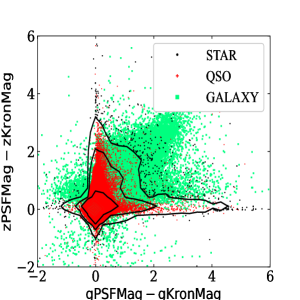
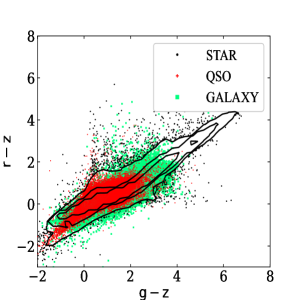
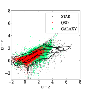
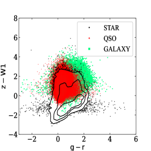
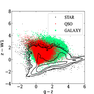
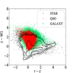
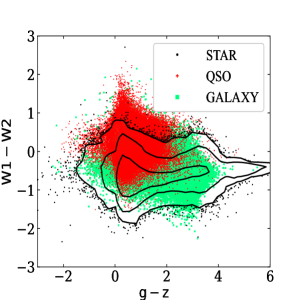
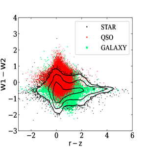
Figure 2: The distribution of stars, galaxies and quasars in 2-d spaces, green filled squares represent galaxies, red pluses represent quasars and black filled circles represent stars. The black outline is the contour of star distribution.

3 The machine learning model

3.1 Introduction to XGBoost

XGBoost (Chen & Guestrin,, 2016) is a boosting algorithm developed on the basis of Gradient Boosting Decision Tree (GBDT) (Friedman et al.,, 2001). It can solve classification and regression problems. Both XGBoost and GBDT apply boosting method to build strong classifiers by means of learning multiple weak classifiers. But XGBoost has an obvious difference from GBDT. When calculating the residual, the first derivative of the loss function is only used for GBDT, while both the first derivative and the second derivative of the loss function are applied for XGBoost. The objective function of XGBoost can be written in the form of Taylor expansion.

$$Obj^{(t)}=\sum_{i=1}^{N}[g_{i}f_{t}(x_{i})+\frac{1}{2}h_{i}f_{t}^{2}(x_{i})]+\Omega(f_{t})$$ (1)

where $g_{i}$ is the first derivative of the loss function, $h_{i}$ is the second derivative of the loss function. The term $\Omega$ defines the complexity of the tree, it can be expressed as

$$\Omega(f_{t})=\gamma T+\frac{1}{2}\lambda\sum_{k=1}^{T}\omega_{k}^{2}$$ (2)

Here $T$ represents the number of leaves, $\omega_{k}$ represents the score given by the $j$th leaf. The learning of the set of functions used in the model is done by minimizing the objective function. Equation (2) helps to smooth the final learnt weights to avoid over-fitting.

For a given data set with $n$ examples and $m$ features $\mathcal{D}=\{(x_{i},y_{i})\}(\left|\mathcal{D}\right|={n},x_{i}\in\mathbb{R}^{m},y_{i}\in\mathbb{R})$. Assumed that the model has $k$ trees totally. The prediction on $x_{i}$ is given by

$$\widehat{y_{i}}=\sum_{k=1}^{K}{f_{k}}(x_{i}),\quad{f_{k}}\in\mathbb{F}$$ (3)

where $f_{k}$ represents one regression tree, and $f_{k}(x_{i})$ is the score that it gives to $x_{i}$. $\mathbb{F}$ is the space of regression trees.

The importance of the XGBoost algorithm has been widely recognized in a number of machine learning and data mining challenges. Recently XGBoost has wide applications in astronomy, such as classification of unknown source in the Fermi-LAT catalogue (Mirabal et al.,, 2016), separation of pulsar signals from noise (Bethapudi & Desai,, 2018), and quasar candidate selection (Jin et al.,, 2019). In this work, we use XGBoost as a supervised learning algorithm to classify galaxies, stars, and quasars from BASS DR3 sources, and XGboost python package was provided by scikit-learn (Pedregosa et al.,, 2011).

3.2 Classification metrics

There are many criteria to score the performance of a classifier. Here, we only apply three standard metrics (Accuracy, Precision and Recall) to determine which classifier is better. Accuracy (short for Accu.) is defined as the fraction of the total number of correct predictions among the total number of predictions, Precision (short for Prec.) is the ratio of true positive predictions to all predicted positive examples, Recall (short for Rec.) is the ratio of true positive predictions to all true positive examples. The confusion matrix is a situation analysis table that summarizes the prediction results of the classification model in machine learning, and describes the data in a matrix form according to the two criteria of the real category and the classification judgement made by the classification model. The confusion matrix is suitable for binary and multiclass classification. Through the confusion matrix, Accuracy, Precision and Recall for each class can be calculated. For our case, how to calculate Accuracy, Precision, Recall for triple classification in a confusion matrix is shown in Table 3.

Table 3: Confusion Matrix

Known$\downarrow$Classified$\to$	GALAXY	QSO	STAR	Precision	Recall
GALAXY	$TG$	$FGQ$	$FGS$	$\displaystyle\frac{TG}{TG+FQG+FSG}$	$\displaystyle\frac{TG}{TG+FGQ+FGS}$
QSO	$FQG$	$TQ$	$FQS$	$\displaystyle\frac{TQ}{TQ+FGQ+FSQ}$	$\displaystyle\frac{TQ}{TQ+FQG+FQS}$
STAR	$FSG$	$FSQ$	$TS$	$\displaystyle\frac{TS}{TS+FGS+FQS}$	$\displaystyle\frac{TS}{TS+FSG+FSQ}$
Total Accuracy	$\displaystyle\frac{TG+TQ+TS}{TG+FGQ+FGS+TQ+FQG+FQS+TS+FSG+FSQ}$
a TG represents the number of actual galaxies that are correctly classified.
b FGQ represents the number of galaxies that are incorrectly classified as quasars.
c FGS represents the number of galaxies that are incorrectly classified as stars.
d TQ represents the number of actual quasars that are correctly classified.
e FQG represents the number of quasars that are incorrectly classified as galaxies.
f FQS represents the number of quasars that are incorrectly classified as stars.
g TS represents the number of actual stars that are correctly classified.
h TSG represents the number of stars that are incorrectly classified as galaxies.
i TSQ represents the number of stars that are incorrectly classified as quasars.

4 The Classifier Model

We randomly divide the known sample into 10 equal subsets keeping the same proportion of the three classes (stars, galaxies and quasars). When training a classifier, we adopt 10-fold cross-validation, which means that 9 subsets are used as training set and the left subset is taken as test set in turn, then the average Accuracy, Precision and Recall are calculated for ten experiments. This work uses XGBoost’s binary classifier (classification of galaxies from stars and quasars) and multiclass classifier (classification of galaxies, stars and quasars) respectively. There are two steps to create classifiers. The first step is to get feature importance by XGBoost, then we try different input patterns of different samples to train XGBoost models and get the best model parameters of XGBoost by grid search. The three main hyper parameters used for XGBoost model optimization include the number of trees in the forest ($n\_estimators$), Maximum depth of a tree ($max\_depth$), Step size shrinkage used in update to prevents overfitting ($learning\_rate$). All other hyper parameters are set with their default values. The second step is to evaluate the performance of different classifiers by ten-fold validation with different input patterns. Finally the best classifiers for different samples are created and then can be applied for prediction of unknown sources. All computing was run in the cloud computing environment of National Astronomical Data Centre (NADC) (Li et al.,, 2017).

4.1 Feature importance

The input pattern is a importance factor to affect the performance of XGBoost. XGBoost may rank relative importance of each feature when used for feature importance analysis according to the gain, which implies the relative contribution of a feature to the XGBoost model. Compared to another feature, the higher gain value of a feature, the more important it is for providing a prediction. Firstly, we evaluate the importance of all possible attributes (${\Delta}g$, ${\Delta}r$, ${\Delta}z$, $g$, $r$, $z$, $g-r$, $r-z$, $g-z$) for optical sample (Sample I) by XGBoost when separating point sources and extended sources (Figure 3 panel (A)) and when discriminating quasars and stars (Figure 3 panel (B)). Secondly, we also assess the importance of all possible attributes (${\Delta}g$, ${\Delta}r$, ${\Delta}z$, $g$, $r$, $z$, $W1$, $W2$, $g-r$, $r-z$, $g-z$, $z-W1$, $g-W1$, $r-W1$, $z-W2$, $g-W2$, $r-W2$, $W1-W2$) for optical and infrared sample (Sample II) by XGBoost when separating point sources and extended sources (Figure 3 panel (C)) and when discriminating quasars and stars (Figure 3 panel (D)). Figure 3 shows that the feature importance is related to samples and classification task. When classifying point sources and extended sources, the rank of feature importance for Sample I is ${\Delta}z$, ${\Delta}r$, ${\Delta}g$, $g-r$, $g$, $g-z$, $r$, $z$, $r-z$; the rank for Sample II is ${\Delta}g$, ${\Delta}z$, $g-W1$, $W1-W2$, $z-W1$, ${\Delta}r$, $g-z$, $z-W2$, $g-r$, $r-z$, $W1$, $r$, $g$, $z$, $r-W2$, $W2$, $r-W1$, $g-W2$. While separating quasars and stars, the rank of feature importance for Sample I is $r$, $g-z$, $z$, $g-r$, ${\Delta}z$, $r-z$, ${\Delta}r$, ${\Delta}g$, $g$; the rank for Sample II is $z-W2$, $W1-W2$, $g-z$, $g-r$, $z-W1$, $r-z$, ${\Delta}z$, $r$, $r-W2$, $z$, ${\Delta}g$, $g-W1$, ${\Delta}r$, $W1$, $g-W2$, $g$, $r-W1$, $W2$. The feature importance is helpful to select effective features for classification. Figure 3 also shows that ${\Delta}g$, ${\Delta}z$, ${\Delta}r$ are very important for distinguishing extended sources from point sources, which is consistent with Figure 1. As shown in Figure 3, $r$, $g-z$, ${\Delta}z$ and ${\Delta}g$ of all features are more important for classification of stars and quasars with optical information; $z-W2$, $W1-W2$, $g-z$ and $g-r$ of all features contribute more to classification of stars and quasars with combined optical and infrared information.

Figure 3: The feature importance with XGBoost. Panel (A) shows the feature importance only with the optical information when classifying extended sources and point sources; panel (B) shows the feature importance only with the optical information when classifying stars and quasars; panel (C) shows the feature importance with combined optical and infrared information when classifying extended sources and point sources; panel (D) shows the feature importance with combined optical and infrared information when classifying stars and quasars.

4.2 Binary classifier construction of XGBoost

We firstly distinguish extended sources (galaxies) from point sources (stars and quasars) by a binary XGBoost classifier. Then the point sources are further classified by another binary XGBoost classifier, and finally the three class labels are assigned to the predicted sample, i.e. we apply two-layer classifiers to realize the classification of galaxies, stars and quasars. After training by grid-search method with all features, we get the best model parameters: $max\-depth=11$, $n\_estimators=100$ and $learning\_rate=0.5$. For the classification of point and extended sources, the classification performance obtained by the different input patterns is shown in Table 4. As indicated in Table 4, the best input pattern is 8-features (${\Delta}g$, ${\Delta}r$, ${\Delta}z$, $g-r$, $g-z$, $r$, $r-z$, $g$) only with optical information for XGBoost. Accuracy is 97.28 per cent, Precision and Recall are more than 96.60 per cent for point sources and extended sources. The optimal input pattern is ${\Delta}g$, ${\Delta}z$, $g-W1$, $W1-W2$, $z-W1$, ${\Delta}r$, $g-z$, $z-W2$, $g-r$,$r-z$,$W1$, $r$, $g$, $z$, $r-W2$ with both optical and infrared information for XGBoost. Accuracy amounts to 98.67 per cent, both Precision and Recall are more than 98.30 per cent for point sources while Precision and Recall are larger than 98.80 per cent for extended sources. Therefore it is reliable to separate extended sources from point sources by XGBoost with optical information or combined optical and infrared information. Moreover it is evident that adding infrared information is helpful to improve classification performance.

Table 4: The performance of binary classifier for point and extended sources

			Point Sources		Extended Sources
Input pattern	Sample	Accu.(%)	Prec.(%)	Rec.(%)	Prec.(%)	Rec.(%)	Time(s)
(${\Delta}g$, ${\Delta}r$, ${\Delta}z$)	Sample I	95.72	94.98	95.75	96.36	95.69	21
(${\Delta}g$, ${\Delta}r$, ${\Delta}z$, $g-r$, $r-z$)	Sample I	96.73	96.07	96.84	97.29	96.63	34
(${\Delta}g$, ${\Delta}r$, ${\Delta}z$, $g-r$, $r-z$, $g-z$)	Sample I	96.78	96.08	96.96	97.39	96.63	47
(${\Delta}g$, ${\Delta}r$, ${\Delta}z$, $g-r$, $r-z$, $r$)	Sample I	97.22	96.57	97.40	97.77	97.06	54
(8-features)	Sample I	97.28	96.63	97.47	97.83	97.11	73
(11-features)	Sample II	98.52	98.26	98.11	98.70	98.80	90
(13-features)	Sample II	98.64	98.35	98.32	98.84	98.86	105
(15-features)	Sample II	98.67	98.39	98.35	98.86	98.89	111
(18-features)	Sample II	98.65	98.37	98.32	98.84	98.87	152
a 8-features represents ${\Delta}g$, ${\Delta}r$, ${\Delta}z$, $g-r$, $g-z$, $r$, $r-z$, $g$.
b 11-features represents ${\Delta}g$, ${\Delta}r$, ${\Delta}z$, $g-r$, $r-z$, $g-z$, $g$, $r$, $z$, $W1$, $W2$.
c 13-features represents ${\Delta}g$, ${\Delta}z$, $g-W1$, $W1-W2$, $z-W1$, ${\Delta}r$, $g-z$, $z-W2$, $g-r$,$r-z$,$W1$, $r$, $g$.
d 15-features represents ${\Delta}g$, ${\Delta}z$, $g-W1$, $W1-W2$, $z-W1$, ${\Delta}r$, $g-z$, $z-W2$, $g-r$,$r-z$,$W1$, $r$, $g$, $z$, $r-W2$.

Then we train the XGBoost classifier on the point sources (stars and quasars), and the classification performance is shown in Table 5. As described in Table 5, the best input pattern is ${\Delta}g$, ${\Delta}r$, ${\Delta}z$, $g-r$, $r-z$, $g-z$, $r$, $g$, $z$ only depending on optical information for XGBoost. Accuracy is 93.22 per cent, Precision and Recall are respectively 93.33 per cent and 93.71 per cent for stars while Precision and Recall are respectively 93.11 per cent and 92.69 per cent for quasars. The optimal input pattern is $z-W2$, $W1-W2$, $g-z$, $g-r$, $z-W1$, $r-z$, ${\Delta}z$, $r$, $r-W2$, $z$, ${\Delta}g$, $g-W1$, ${\Delta}r$, $W1$, $g-W2$ with both optical and infrared information for XGBoost. Accuracy amounts to 99.15 per cent, Precision and Recall are respectively 99.00 per cent and 99.46 per cent for stars while Precision and Recall are respectively 99.33 per cent and 98.77 per cent for quasars. In terms of Accuracy, Precision and Recall, XGBoost classifiers are effective to separate quasars from stars with optical information or combined optical and infrared information. As expected, adding infrared information contributes to classification performance.

Table 5: The performance of binary classifier for stars and quasars by XGBoost.

			STAR		QSO
Input pattern	Sample	Accu.(%)	Prec.(%)	Rec.(%)	Prec.(%)	Rec.(%)	Time(s)
(${\Delta}g$, ${\Delta}r$, ${\Delta}z$, $g-r$)	Sample I	84.68	83.13	88.62	86.62	80.38	12
($r$, $g-z$,$z$,$g-r$)	Sample I	91.31	91.40	91.99	91.20	90.56	17
($r$, $g-r$,$r-z$)	Sample I	91.75	91.71	92.55	91.79	90.87	12
(${\Delta}g$, ${\Delta}r$, ${\Delta}z$, $g-r$, $r-z$, $r$)	Sample I	93.20	93.25	93.75	93.14	92.60	25
(9-features)	Sample I	93.22	93.33	93.71	93.11	92.69	37
($g-r$, $r-z$, $r$, $g$, $z$, $w1$, $w2$)	Sample II	98.88	98.61	99.38	99.23	98.27	24
(10-features)	Sample II	99.11	98.95	99.45	99.32	98.70	29
(12-features)	Sample II	99.13	98.92	99.51	99.40	98.67	17
(15-features)	Sample II	99.15	99.00	99.46	99.33	98.77	25
(17-features)	Sample II	99.12	98.94	99.47	99.35	98.69	36
a 9-features represents ${\Delta}g$, ${\Delta}r$, ${\Delta}z$, $g-r$, $r-z$, $g-z$, $r$, $g$, $z$.
b 10-features represents $z-W2$,$z-W1$, $g-r$, $W1-W2$, ${\Delta}z$,${\Delta}g$, ${\Delta}r$, $r-z$, $r-W2$, $r$.
c 12-features represents $z-W2$,$z-W1$, $g-z$, $W1-W2$, $g-r$, ${\Delta}z$, $r-z$, $r-W2$, $r$, $z$, ${\Delta}g$, $g-W1$.
d 15-features represents $z-W2$, $W1-W2$, $g-z$, $g-r$, $z-W1$, $r-z$, ${\Delta}z$, $r$, $r-W2$, $z$, ${\Delta}g$, $g-W1$, ${\Delta}r$, $W1$, $g-W2$.
e 17-features represents $z-W2$,$z-W1$, $g-z$, $W1-W2$, $g-r$, ${\Delta}z$, $r-z$, $r-W2$, $r$, $z$, ${\Delta}g$, $g-W1$, ${\Delta}r$, $g$, $g-W2$, $W1$, $W2$.

According to the above experimental results, the difference between $PSFMag$ and $KronMag$ in $g$, $r$, and $z$ bands has great impact on the distinction between point and extended sources, while for the classification of stars and quasars, the infrared features $W1$, $W2$ are very important. When using two-layer binary classifiers, the first-layer classification performance will also affect the second-layer classification prediction. Considering running time, XGBoost is a fast algorithm for classification and shows its superiority in dealing with large scale data.

4.3 Multiclass classifier construction of XGBoost

Compared with two-layer binary classifiers, it is simple to use multiclass classifier to classify galaxies, stars and quasars. For multiclass classifier, you only need to set $objective$ to $multi:softmax$ and $num\_class$ to 3 in the XGBoost model. The basic training process is exactly the same as the binary classifier model training. We use the grid search method to get the optimal model parameters and 10-fold cross validation to get average Accuracy, Precision and Recall values. The best model parameters for XGBoost are $max\-depth=7$, $n\_estimators=200$ and $learning\_rate=0.5$ According to the confusion matrix, we calculate the classification Accuracy, Precision and Recall for each class. Table 6 shows the performance of multi-class classifiers with four kinds of input patterns for classification of galaxies, stars and quasars. As shown in Table 6, there are two input patterns for the samples only with optical information: input pattern I for ${\Delta}g$, ${\Delta}r$, ${\Delta}z$, $g-r$, $r-z$, $r$ and input pattern II for ${\Delta}g$, ${\Delta}r$, ${\Delta}z$, $g-r$, $g-z$, $r$, $r-z$, $z$; also two input patterns for the samples with both optical and infrared information, input pattern III for $z-W2$, ${\Delta}z$, $W1-W2$, ${\Delta}r$, $g-r$, $z-W1$, $W1$, $W2$ and input pattern IV for $z-W2$, ${\Delta}z$, $W1-W2$, ${\Delta}r$, $g-r$, $z-W1$, ${\Delta}g$, $g-z$, $r-W2$, $r-z$, $r$. Comparing the performance of input pattern II with that of input pattern I, Accuracy is better (94.49 per cent vs. 94.47 per cent), Precision and Recall are better for stars and galaxies, Recall is better and Precision is a little worse for quasars. Considering all these, the performance of input pattern II is a little superior to that of input pattern I. Comparing the performance of input pattern IV with that of input pattern III, Accuracy is better (98.43 per cent vs. 97.90 per cent), Precision and Recall are all better for stars, galaxies and quasars. Given these, the performance of input pattern IV outperforms that of input pattern III.

Table 6: The performance of multi-class classifier for galaxies, stars and quasars.

			GALAXY		STAR		QSO
Input pattern	Sample	Accu.(%)	Prec.(%)	Rec.(%)	Prec.(%)	Rec.(%)	Prec.(%)	Rec.(%)	Time(s)
Input pattern I	Sample I	94.47	97.74	97.32	92.96	90.59	88.68	91.63	326
Input pattern II	Sample I	94.49	97.76	97.34	93.00	90.60	88.67	91.65	260
Input pattern III	Sample II	97.90	98.36	98.76	98.32	95.50	96.37	97.62	160
Input pattern IV	Sample II	98.43	98.85	98.97	98.74	97.28	97.07	97.95	330
a Input pattern I represents ${\Delta}g$, ${\Delta}r$, ${\Delta}z$, $g-r$, $r-z$, $r$.
b Input pattern II represents ${\Delta}g$, ${\Delta}r$, ${\Delta}z$, $g-r$, $g-z$, $r$, $r-z$, $z$.
c Input pattern III represents $z-W2$, ${\Delta}z$, $W1-W2$, ${\Delta}r$, $g-r$, $z-W1$, $W1$, $W2$.
d Input pattern IV represents $z-W2$, ${\Delta}z$, $W1-W2$, ${\Delta}r$, $g-r$, $z-W1$, ${\Delta}g$, $g-z$, $r-W2$, $r-z$, $r$.

4.4 Discussion

Our goal is to separate galaxies, stars and quasars with photometric data (BASS optical filters: $g$, $r$, $z$; ALLWISE mid-IR: $W1$, $W2$) using XGBoost. In their optical images, galaxies are easily discriminated from stars and quasars due to their extended morphology. As described in Figure 1, the extended characteristics of galaxies is distinct in ${\Delta}z$, ${\Delta}r$ and ${\Delta}g$ whose absolute values are not zero; stars and quasars are similar and pointed, and the absolute values of ${\Delta}z$, ${\Delta}r$ and ${\Delta}g$ for them are near zero. From Figure 2, it is known that galaxies, stars and quasars are difficult to separate from each other with one or two of all the features although their separation improves a lot with the additional infrared information and their overlapping still exists.

Compared to 1-d histogram and 2-d scatter plot, XGBoost may take all features into account and solve the classification problem. As shown in Tables 4-6, it is concluded that the classification accuracy increases for any classifier when adding the information from infrared band. The best performance is obtained with all information from optical and infrared bands. If one source is predicted both by classifiers with optical information and by those with combined optical and infrared information, the predicted results by classifiers with combined optical and infrared information are more reliable than those by classifiers with optical information, the same predicted results by all these classifiers is the most reliable. As shown in Table 4, Figure 1 and Figure 3, ${\Delta}z$, ${\Delta}r$ and ${\Delta}g$ are of great importance for separation of extended and point sources (Accuracy: more than 95.70 per cent) no matter for Sample I or Sample II, the infrared information influence the performance of a classifier to some extent. As indicated in Figure 3 and Table 5, the four important features ($r$, $g-z$, ${\Delta}z$ and ${\Delta}g$) for Sample I are different from those ($z-W2$, $W1-W2$, $g-z$ and $g-r$) for Sample II, the performance of a classifier improve a lot from 93.22 per cent to 99.15 per cent with additional infrared information when distinguishing stars and quasars. As a result, the infrared information had better be considered as possible when targeting quasar candidates, especially obscured quasars not identified only by optical information.

Stern et al., (2005) and Hickox et al., (2007) pointed out that infrared information is efficient to discriminate quasars. Bovy et al., (2012) and DiPompeo et al., (2015) showed the power of infrared information for targeting quasar candidates using Extreme deconvolution (XD). Our work further proves that infrared information is of great importance to single out quasar candidates by photometric data.

Comparing the best results by two-layer binary classifiers in Tables 4-5 with those by multiclass classifier in Table 6, no matter with optical information or both optical and infrared information, Precision and Recall of quasars and stars by two-layer binary classifiers are better than those by multiclass classifier; however for galaxies, Recall of multiclass classifier is superior to that of two-layer binary classifiers, while Precision of two-layer binary classifiers outperforms that of multiclass classifier. As a result, predicted results by two-layer binary classifiers are more reliable for quasars and stars; predicted results by two-layer binary classifier are more trustworthy for galaxies in terms of Precision.

Except XGBoost, there are various methods used for celestial object classification, such as random forest, support vector machine (SVM). Table 7 shows the performance of random forest for classification of stars and quasars with Sample I and Sample II. For sample I, the better performance is obtained with 9-features (${\Delta}g$, ${\Delta}r$, ${\Delta}z$, $g-r$, $r-z$, $g-z$, $r$, $g$, $z$); only given Accuracy, the best input pattern is 9-features (Accuracy: 93.27 per cent). For Sample II, the best performance is achieved with 15-features (Accuracy: 99.14 per cent); Precision is 98.82 per cent and 99.53 per cent respectively for stars and quasars; Recall is 99.62 per cent and 98.54 per cent separately for stars and quasars. Comparing the results in Table 7 with those in Table 5, it is found that the performance of XGBoost is comparative to that of random forest whether for Sample I or Sample II and the running time of XGBoost is shorter than that of random forest. As a result, XGBoost outperforms random forest for our case in terms of efficiency.

Table 7: The performance of binary classifier for stars and quasars by Random Forest.

			STAR		QSO
Input pattern	Sample	Accu.(%)	Prec.(%)	Rec.(%)	Prec.(%)	Rec.(%)	Time(s)
(${\Delta}g$, ${\Delta}r$, ${\Delta}z$, $g-r$)	Sample I	85.51	83.52	89.99	88.07	80.63	125
(${\Delta}g$, ${\Delta}r$, ${\Delta}z$, $g-r$, $r-z$, $r$)	Sample I	93.17	92.31	94.81	94.16	91.39	120
(9-features)	Sample I	93.27	92.83	94.39	93.77	92.05	180
($g-r$, $r-z$, $r$, $g$, $z$, $w1$, $w2$)	Sample II	98.77	98.24	99.55	99.44	97.81	80
(15-features)	Sample II	99.14	98.82	99.62	99.53	98.54	120
a 9-features represents ${\Delta}g$, ${\Delta}r$, ${\Delta}z$, $g-r$, $r-z$, $g-z$, $r$, $g$, $z$.
b 12-features represents $z-W2$,$z-W1$, $g-z$, $W1-W2$, $g-r$, ${\Delta}z$, $r-z$, $r-W2$, $r$, $z$, ${\Delta}g$, $g-W1$.
b 15-features represents $z-W2$,$W1-W2$,$g-z$,$g-r$,$z-W1$,$r-z$,${\Delta}z$,$r$,$r-W2$,$z$,${\Delta}g$,$g-W1$,${\Delta}r$,$W1$,$g-W2$.

5 Application of Classifiers

According to the above experimental results for the known samples, we construct six classifier models, the detailed information is shown in Table 8. If the binary classification model is adopted, two binary classifiers are needed to finish classification of galaxies, stars and quasars, the first classifier separates galaxies from stars and quasars, the second discriminates quasars and stars. While using the multiclass classification model, it only needs one multiclass classifier to finish classification of galaxies, stars and quasars. For each classifier, the optimal patterns obtained from above experiments are applied for different samples.

Table 8: The six classifiers of XGBoost constructed

Classifier	objective	Input pattern	Class
Classifier $1^{st}$	binary:logistic	(${\Delta}g$, ${\Delta}r$, ${\Delta}z$, $g-r$, $g-z$, $r$, $r-z$, $g$)	(point and extended sources)
Classifier $2^{nd}$	binary:logistic	(${\Delta}g$, ${\Delta}r$, ${\Delta}z$, $g-r$, $r-z$, $g-z$, $r$, $g$, $z$)	(stars and quasars)
Classifier $3^{rd}$	multi:softmax	(${\Delta}g$, ${\Delta}r$, ${\Delta}z$, $g-r$, $g-z$, $r$, $r-z$, $z$ )	(galaxies, stars and quasars)
Classifier $4^{th}$	binary:logistic	(Pattern I)	(point and extended sources)
Classifier $5^{th}$	binary:logistic	(Pattern II)	(stars and quasars)
Classifier $6^{th}$	multi:softmax	(Pattern III)	(galaxies, stars and quasars)
a Extended sources represent galaxies while point sources for stars and quasars.
b Pattern I represents ${\Delta}g$, ${\Delta}z$, $g-W1$, $W1-W2$, $z-W1$, ${\Delta}r$, $g-z$, $z-W2$, $g-r$,$r-z$,$W1$, $r$, $g$, $z$, $r-W2$.
c Pattern II represents $z-W2$,$W1-W2$,$g-z$,$g-r$,$z-W1$,$r-z$,${\Delta}z$,$r$,$r-W2$,$z$,${\Delta}g$,$g-W1$,${\Delta}r$,$W1$,$g-W2$.
d Pattern III represents $z-W2$, ${\Delta}z$, $W1-W2$, ${\Delta}r$, $g-r$, $z-W1$, ${\Delta}g$, $g-z$, $r-W2$, $r-z$, $r$.

After constructing these classifiers, we use these classifiers to predict BASS DR3 sources. Figure 4 shows the classification workflow. The red rectangle boxes indicate data analysis and black parallelograms represent intermediate data or results.

Figure 4: The classification workflow.

According to Figure 4, BASS-DR3 sources (110 896 598) are firstly classified into extended sources (galaxies) and point sources (stars and quasars) by Classifier $1^{st}$, then the point sources are further separated into stars and quasars by Classifier $2^{nd}$. BASS-DR3 sources are also directly divided into galaxies, stars and quasars by Classifier $3^{rd}$. By correlating BASS-DR3 sources with ALLWISE database, we obtain BASS-DR3-ALLWISE sources (43 859 467). Similar to classifying BASS DR3 sources, BASS-DR3-ALLWISE sources are firstly grouped into extended sources (galaxies) and point sources (stars and quasars) by Classifier $4^{th}$, then the point sources are further discriminated into stars and quasars by Classifier $5^{th}$. BASS-DR3-ALLWISE sources are directly distinguished into galaxies, stars and quasars by Classifier $6^{th}$. Each prediction includes predicted classification label and likelihood. If the classification given by binary classifiers is the same as that by multiclass classifiers, the classification is more reliable. When classification is both provided by classifiers from optical information and classifiers from both optical and infrared information, the classification result is much trustier by classifiers from combined optical and infrared information. If only considering the results by binary classifier or multiclass classifier, the predicted results from two-layer binary classifier are adopted for quasars and stars; but for galaxies, the predicted results from two-layer binary classifiers are fit in terms of Precision while those form multiclass classifier are fit in terms of Recall.

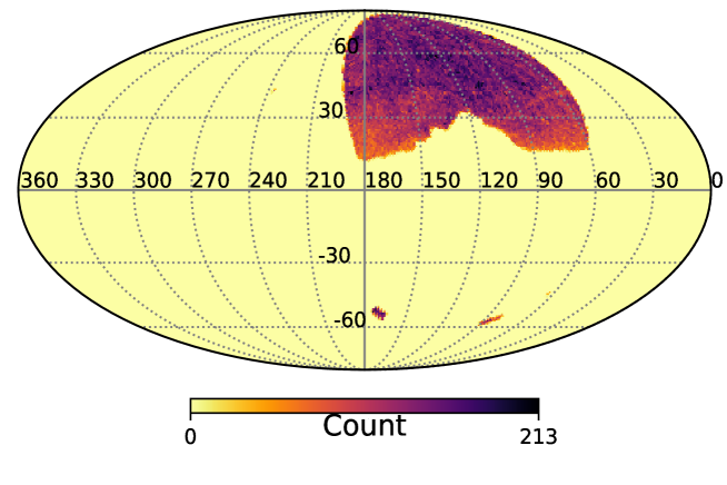
Figure 6: The galactic location of quasar candidates with larger than 95 per cent probability by binary&multiclass classifiers based on optical and infrared information.

For the BASS DR3 sources, all predicted results are combined in a whole table. The link address is http://paperdata.china-vo.org/Li.Changhua/bass/bassdr3-label-catalogue. Table 9 lists the 20 rows of predicted results, which is of great value for the further research on the characteristics and physics of BASS DR3 sources. The number of star, galaxy and quasar candidates by different classifiers with different information is shown in Table 10. When only using optical information, the BASS-DR3 sources simultaneously assigned as stars, galaxies and quasars by all classifiers respectively adds up to 19 829 533 ($P_{\rm S}>0.75$), 49 483 839 ($P_{\rm G}>0.75$) and 7 095 580 ($P_{\rm Q}>0.75$), among which quasar candidates with $P_{\rm Q}>0.90$ and $P_{\rm Q}>0.95$ amount to 2 775 970 and 1 166 517, respectively. When applying both optical and infrared information with the same predicted results by binary and multiclass classifiers, the number of star candidates is 12 785 232 ($P_{\rm S}>0.75$), 12 561 500 ($P_{\rm S}>0.90$) and 12 375 838 ($P_{\rm S}>0.95$); the number of galaxy candidates is 25 068 898 ($P_{\rm G}>0.75$), 21 890 547 ($P_{\rm G}>0.90$) and 18 606 073 ($P_{\rm G}>0.95$); the number of quasar candidates is 1 500 099 ($P_{\rm Q}>0.75$), 1 033 486 ($P_{\rm Q}>0.90$) and 798 928 ($P_{\rm Q}>0.95$). If only considering the completeness, we may combine the predicted results by binary and multiclass classifiers. Touching upon reliability, we adopt the same classified results by binary and multiclass classifiers only with optical information as those with both optical and infrared information. At this situation, the total number of quasar candidates is 1 262 964, among which there are 694 260 ($P_{\rm Q}>0.75$), 375 591 ($P_{\rm Q}>0.90$), 235 713 ($P_{\rm Q}>0.95$). As shown in Table 10 for larger than 95 per cent probability (i.e. both $P_{b1}$ and $P_{b2}$ above 95 per cent or both $P_{bi1}$ and $P_{bi2}$ above 95 per cent for two-layer binary classifiers, $P_{m}$ or $P_{mi}$ above 95 per cent for multiclass classifiers), the number of quasar candidates meanwhile by binary and multiclass classifiers is about 233 per deg² only with optical information, while the number of quasar candidates by binary, multiclass and binary&multiclass classifiers is respectively about 218, 189 and 160 per deg² with optical and infrared information, which is consistent with the quasar luminosity function (Palanque-Delabrouille et al.,, 2016; Wilson & White,, 1995). Based on optical and infrared information, the number of quasar candidates by binary classifier with different probabilities and those with larger than 95 per cent probability by different classifiers as function of $r$ magnitude are displayed in Figure 5 and the galactic location of the quasar candidates with larger than 95 per cent probability by binary&multiclass classifiers is demonstrated in Figure 6. The number of quasar candidates decreases when $r>23$, which results from the number decrease of observed BASS sources as $r>23$. As shown in Figure 6, most of quasar candidates distribute on medium and high latitude, and there is no accumulation of quasar candidates along the galactic plane.

Table 9: Predicted results of BASS DR3 sources.

id	ra	dec	Class$\_b$	$P_{b1}$	$P_{b2}$	Class$\_m$	$P_{m}$	Class$\_bi$	$P_{bi1}$	$P_{bi2}$	Class$\_mi$	$P_{mi}$
95373011289	135.04541765729505	84.39853006107745	0	0.992	0.993	0	0.981	0	0.997	1.000	0	0.999
95373012270	137.06618290826282	84.45571948189149	0	0.999	0.965	0	0.994	0	0.999	0.978	0	0.993
95373014038	135.24278336054908	84.55902133199768	0	0.962	0.999	0	0.963	0	1.000	1.000	0	0.998
95374009915	145.63427167809962	84.3344909394295	0	0.976	0.999	0	0.980	0	0.956	0.999	0	0.993
95374010728	145.64322900143938	84.37462462607955	0	0.997	0.993	0	0.956	0	1.000	1.000	0	0.993
95375006879	146.35493428612986	84.18153150948889	0	0.999	0.996	0	0.983	0	1.000	1.000	0	1.000
95375008769	146.7341471886791	84.28327327388713	0	0.963	0.980	0	0.970	0	0.999	1.000	0	0.998
95375010415	146.783645308867	84.37315314289253	0	0.999	0.936	0	0.943	0	1.000	1.000	0	0.999
95371004745	123.71207464080723	84.1579130418392	1	1.000	0.998	1	0.999	1	1.000	1.000	1	1.000
95371004752	123.76995258941326	84.15844883612738	1	0.989	0.996	1	0.961	1	0.998	0.999	1	0.997
95371005233	123.80162434791758	84.18398863492929	1	0.999	0.999	1	0.998	1	1.000	1.000	1	1.000
95371005325	123.79929150615568	84.18879820615973	1	0.996	0.938	1	0.963	1	0.999	0.999	1	0.999
95371005366	123.70596853052086	84.19100324818724	1	0.970	0.997	1	0.970	1	0.972	0.997	1	0.998
95371005498	123.91422908428144	84.19767799033559	2	0.965		2	0.952	2	0.946		2	0.968
95371005594	123.61974576953872	84.2038370079812	2	0.960		2	0.974	2	0.991		2	0.991
95371005759	123.91886392365679	84.21438506899153	2	0.995		2	0.995	2	0.951		2	0.990
95371005789	123.15220933495931	84.21426532956772	2	0.986		2	0.978	2	0.995		2	0.974
95371005812	123.77907625197672	84.21706698284555	2	0.995		2	0.991	2	0.996		2	0.983
95371005951	123.84673982200142	84.22579958818966	2	0.973		2	0.988	2	0.998		2	0.988
95371005960	123.77794020713335	84.22598315903795	2	0.912		2	0.970	2	0.994		2	0.991
a Class_b is the classification label, $P_{b1}$ and $P_{b2}$ are respectively their classification probabilities by Classifier $1^{st}$ and Classifier $2^{nd}$;
b Class_m is the classification label, $P_{m}$ is their classification probabilities by Classifier $3^{rd}$ ;
c Class_bi is the classification label, $P_{bi1}$ and $P_{bi2}$ are respectively their classification probabilities by Classifier $4^{th}$ and Classifier $5^{th}$ ;
d Class_mi is the classification label, $P_{mi}$ is their classification probabilities by Classifier $6^{th}$.
e The classification label definition: 0 represents quasars, 1 represents stars and 2 represents galaxies.
f Note for the sources assigned as galaxies, $P_{b2}$ or $P_{bi2}$ is default.
g This catalogue files is available in http://paperdata.china-vo.org/Li.Changhua/bass/bassdr3-label-catalogue.
h A portion is shown here for guidance regarding its form and content.

Table 10: Star, galaxy and quasar candidates by different classifiers with different information.

Information		Optical			Optical&infrared
Classifier	Binary	Multiclass	Binary&Multiclass	Binary	Multiclass	Binary&Multiclass
$P_{\rm S}>0.75$	21 175 837	20 550 441	19 829 533	12 938 789	12 913 835	12 785 232
$P_{\rm S}>0.90$	18 570 067	17 759 188	17 043 293	12 697 599	12 711 753	12 561 500
$P_{\rm S}>0.95$	16 706 080	15 727 548	15 022 399	12 519 421	12 560 931	12 375 838
$P_{\rm G}>0.75$	54 360 301	56 235 525	49 483 839	25 929 229	26 490 981	25 068 898
$P_{\rm G}>0.90$	41 243 840	41 713 806	35 544 793	23 417 967	23 899 117	21 890 547
$P_{\rm G}>0.95$	32 053 408	31 025 081	25 949 348	20 888 403	21 088 855	18 606 073
$P_{\rm Q}>0.75$	11 575 871	9 459 579	7 095 580	2 078 981	1 777 386	1 500 099
$P_{\rm Q}>0.90$	5 271 397	4 052 081	2 775 970	1 419 024	1 221 362	1 033 486
$P_{\rm Q}>0.95$	2 674 704	1 874 389	1 166 517	1 088 976	943 486	798 928
a $P_{\rm S}$ is the probabilities that sources are identified as stars, e.g. $P_{b1}$ and $P_{b2}$ are meanwhile above 95 percent if $P_{\rm S}>0.95$
for optical sample, $P_{bi1}$ and $P_{bi2}$ are meanwhile above 95 percent if $P_{\rm S}>0.95$ for optical and infrared sample;
b $P_{\rm G}$ is the probabilities that sources are identified as galaxies, e.g. $P_{b1}$ is above 95 percent if $P_{\rm G}>0.95$ for optical sample,
$P_{bi1}$ is above 95 percent if $P_{\rm G}>0.95$ for optical and infrared sample;
c $P_{\rm Q}$ is the probabilities that sources are identified as quasars, e.g. $P_{b1}$ and $P_{b2}$ are meanwhile above 95 percent if $P_{\rm Q}>0.95$
for optical sample, $P_{bi1}$ and $P_{bi2}$ are meanwhile above 95 percent if $P_{\rm Q}>0.95$ for optical and infrared sample.

Figure 5: Left panel: the number of quasar candidates by binary classifier with optical and infrared information as function of $r$ magnitude for different probabilities ($P_{Q}>0.95$ (red dotted line), $P_{Q}>0.90$ (blue dash line), $P_{Q}>0.75$ (green dotted dash line, all (black line)); right panel: the number of quasar candidates as function of $r$ magnitude with larger than 95 per cent probability by binary&multiclass (red dotted line), binary (blue dash line), multiclass (green dotted dash line) and binary/multiclass (black line) classifiers based on optical and infrared information.

6 Conclusions

It is hard to discriminate stars, galaxies and quasars only depending on single feature or two of all features. Facing classification in a high dimensional space, machine learning is a good choice. Our experimental results show that XGBoost classifiers get more efficient than colour cut or colour-colour plot, and are comparable to random forest on the classification of celestial objects. As for classification of more than two classes, multiclass classifier or multi-layer binary classifiers may perform; for our case, three-class classifier and two-layer binary classifiers are applied. We construct six classifiers to predict classification label and their probabilities with different input patterns for BASS-DR3 sources. The predicted results from different classifiers and original properties are listed in a whole table, which may shed light on further research about source properties of various kinds of objects in detail. The sources labelled as quasars will be taken as input catalogue of LAMOST, DESI or other projects for follow-up observation. With the future implementation of BASS survey, we may predict the new sources from the new survey by our classifiers or new classifiers created by more known spectroscopic objects. If only interested in some special objects, we may use machine learning to create the classifier of special objects and choose special object candidates for further study.

7 Acknowledgements

We are very grateful to the referees for their constructive suggestions to help us improve our paper. This work is supported by National Natural Science Foundation of China (NSFC)(11573019, 11803055, 11873066), the Joint Research Fund in Astronomy (U1531246, U1731125, U1731243, U1731109) under cooperative agreement between the NSFC and Chinese Academy of Sciences (CAS), the 13th Five-year Informatization Plan of Chinese Academy of Sciences (No. XXH13503-03-107). We would like to thank the National R&D Infrastructure and Facility Development Program of China, “Earth System Science Data Sharing Platform” and “Fundamental Science Data Sharing Platform” (DKA2017-12-02-07). Data resources are supported by Chinese Astronomical Data Center (NADC) and Chinese Virtual Observatory (China-VO). This work is supported by Astronomical Big Data Joint Research Center, co-founded by National Astronomical Observatories, Chinese Academy of Sciences and Alibaba Cloud. This research has made use of BASS DR3 catalogue. BASS is a collaborative program between the National Astronomical Observatories of the Chinese Academy of Science and Steward Observatory of the University of Arizona. It is a key project of the Telescope Access Program (TAP), which has been funded by the National Astronomical Observatories of China, the Chinese Academy of Sciences (the Strategic Priority Research Program. The Emergence of Cosmological Structures grant no. XDB09000000), and the Special Fund for Astronomy from the Ministry of Finance. BASS is also supported by the External Cooperation Program of the Chinese Academy of Sciences (grant No. 114A11KYSB20160057) and the Chinese National Natural Science Foundation (grant No. 11433005). The BASS data release is based on the Chinese Virtual Observatory (China-VO). The Guoshoujing Telescope (the Large Sky Area Multi-object Fiber Spectroscopic Telescope, LAMOST) is a National Major Scientific Project built by the Chinese Academy of Sciences. Funding for the project has been provided by the National Development and Reform Commission. LAMOST is operated and managed by the National Astronomical Observatories, Chinese Academy of Sciences.

We acknowledgment SDSS databases. Funding for the Sloan Digital Sky Survey IV has been provided by the Alfred P. Sloan Foundation, the U.S. Department of Energy Office of Science, and the Participating Institutions. SDSS-IV acknowledges support and resources from the Center for High-Performance Computing at the University of Utah. The SDSS web site is www.sdss.org. SDSS-IV is managed by the Astrophysical Research Consortium for the Participating Institutions of the SDSS Collaboration including the Brazilian Participation Group, the Carnegie Institution for Science, Carnegie Mellon University, the Chilean Participation Group, the French Participation Group, Harvard-Smithsonian Center for Astrophysics, Instituto de Astrofísica de Canarias, The Johns Hopkins University, Kavli Institute for the Physics and Mathematics of the Universe (IPMU) /University of Tokyo, Lawrence Berkeley National Laboratory, Leibniz Institut für Astrophysik Potsdam (AIP), Max-Planck-Institut für Astronomie (MPIA Heidelberg), Max-Planck-Institut für Astrophysik (MPA Garching), Max-Planck-Institut für Extraterrestrische Physik (MPE), National Astronomical Observatories of China, New Mexico State University, New York University, University of Notre Dame, Observatário Nacional / MCTI, The Ohio State University, Pennsylvania State University, Shanghai Astronomical Observatory, United Kingdom Participation Group, Universidad Nacional Autónoma de México, University of Arizona, University of Colorado Boulder, University of Oxford, University of Portsmouth, University of Utah, University of Virginia, University of Washington, University of Wisconsin, Vanderbilt University, and Yale University.

8 Data availability

The predicted results for BASS-DR3 sources is saved in a repository and can be obtained by a unique identifier, part of which is indicated in Table 9. It is put in paperdata at http://paperdata.china-vo.org, and can be available with http://paperdata.china-vo.org/Li.Changhua/bass/bassdr3-label-catalogue.

References

- Arnason et al., (2020) Arnason R. M., Barmby P., Vulic N., 2020, MNRAS, 492, 5075
- Bethapudi & Desai, (2018) Bethapudi S., Desai S., 2018, Astron. Comput., 23, 15
- Bilickiet et al., (2018) Bilicki M. et al., 2018, A&A, 616, A69
- Blanton et al., (2017) Blanton M. R. et al., 2017, AJ, 154, 28
- Bovy et al., (2012) Bovy J. et al., 2012, ApJ, 749, 41
- Boyle et al., (1990) Boyle B. J., Fong R., Shanks T., Peterson, B. A., 1990, MNRAS, 243, 1
- Brad et al., (2020) Brad W. Lyke et al., 2020, ApJS, 250, 8
- Brandt & Hasinger, (2005) Brandt W. N., Hasinger G., 2005, ARA&A, 43, 727
- Breiman, (2001) Breiman L. 2001, Machine Learning, 45, 5
- Broos et al., (2011) Broos P. S., Getman K. V., Povich M. S., Townsley L. K., 2011, ApJS, 194, 4
- Cui et al., (2012) Cui X.-Q. et al. 2012, RAA, 12, 1197
- Chen & Guestrin, (2016) Chen T., Guestrin C., 2016, Proceedings of the 22nd ACM SIGKDD International Conference on Knowledge Discovery and Data Mining. ACM
- Clarke et al., (2020) Clarke A. O. A., Scaife M. M., Greenhalgh R., Griguta V., 2020, A&A, 639, A84
- Connor & van Leeuwen, (2018) Connor L., van Leeuwen J., 2018, AJ, 156, 256
- DiPompeo et al., (2015) DiPompeo M. A., Bovy J., Myers A. D., Lang D., 2015, MNRAS, 452, 3124
- Eisenstein et al., (2011) Eisenstein D. J. et al. 2011, AJ, 142, 72
- Farah et al., (2018) Farah W. et al., 2018, MNRAS, 478, 1209
- Farah et al., (2019) Farah W. et al., 2019, MNRAS, 488, 2989
- Florios et al., (2018) Florios K., Kontogiannis I., Park S.-H., Guerra J. A., Benvenuto F., Bloomfield D. S., Georgoulis M. K., 2018, Solar Physics, 293, 28
- Friedman et al., (2000) Friedman J., Hastie T., Tibshirani R., 2000, The Annals of Statistics, 28(2), 337
- Friedman et al., (2001) Friedman J. H., 2001, Ann. Stat., 29, 1189
- Gao et al., (2008) Gao D., Zhang Y., Zhao Y., 2008, MNRAS, 386(3), 1417
- (23) George D., Huerta E. A., 2018, Physics Letters B, 778, 64
- (24) George D., Huerta E. A., 2018, Physical Review D, 97, 044039
- Gregg et al., (1996) Gregg M. D., Becker R. H., White R. L., Helfand D. J., McMahon R. G., Hook I. M., 1996, AJ, 112, 407
- Hewett et al., (1995) Hewett P. C., Foltz C. B., Chaffee F. H., 1995, AJ, 109, 1498
- Hewett et al., (2001) Hewett P. C., Foltz C. B., Chaffee F. H., 1995, AJ, 122, 518
- Hickox et al., (2007) Hickox R. C. et al., 2007, ApJ, 671, 1365
- Inceoglu et al., (2018) Inceoglu F., Jeppesen J. H., Kongstad P., Hernndez Marcano, N. J., Jacobsen, R. H., Karoff, C., 2018, AJ, 861, 128
- Jacobs et al., (2017) Jacobs C., Glazebrook K., Collett T., More A., McCarthy C., 2017, MNRAS, 471, 167
- Jin et al., (2019) Jin X., Zhang Y., Zhang J., Zhao Y., Wu X.-B., Fan D., 2019, MNRAS, 485, 4539
- Lanusse et al., (2018) Lanusse F., Ma Q., Li N., Collett, T. E., Li C.-L., Ravanbakhsh S., Mandelbaum R., Poczos B., 2018, MNRAS, 473, 3895
- Li et al., (2017) Li C. et al., 2017, Astroinformatics, Proceedings of the International Astronomical Union, IAU Symposium, 325, 353
- Luo et al., (2015) Luo A. L. et al., 2015, RAA, 15, 1095
- Mahabal et al., (2019) Ashish M. et al., 2019, PASP, 131, 997
- Miller & Coe, (1996) Miller A. S., Coe M. J., 1996, MNRAS, 279, 293
- Mirabal et al., (2016) Mirabal N., Charles E., Ferrara E. C., Gonthier P. L., Harding A. K., Sanchez-Conde M. A., Thompson D. J., 2016, ApJ, 825, 69
- Nishizuka et al., (2017) Nishizuka N., Sugiura K., Kubo Y., Den M., Watari S., Ishii M., 2017, AJ, 835, 156
- Odewahn et al., (1994) Odewahn S. C., Nielsen, M. L., 1994, Vistas in Astronomy, 38, 281
- Palanque-Delabrouille et al., (2016) Palanque-Delabrouille N. et al., 2016, A&A, 587, A41
- Pris et al., (2018) Pris I. et al., 2018, A&A, 613, A51
- Pearson et al., (2018) Pearson K. A., Palafox L., Griffith C. A., 2018, MNRAS, 474, 478
- Peng et al., (2012) Peng N., Zhang Y., Zhao Y., Wu X.-B, 2012, MNRAS, 425, 2599
- Pourrahmani et al., (2018) Pourrahmani M., Nayyeri H., Cooray A., 2018, ApJ, 856, 68
- Powell et al., (2017) Powell J., Torres-Forne A., Lynch R. et al., 2017, Classical and Quantum Gravity, 34, 034002?
- Pedregosa et al., (2011) Pedregosa F. et al., 2011, Journal of Machine Learning Research, 12, 2825
- Rodriguez et al., (2006) Rodriguez J. J., Kuncheva L. I., Alonso C. J., 2006, IEEE Transactions on Pattern Analysis and Machine Intelligence, 28(10), 1619
- Ruiz et al., (2018) Ruiz A., Corral A., Mountrichas G., Georgantopoulos I., 2018, A&A, 618, A52
- Santos-LIeo et al., (2009) Santos-LIeo M., Schartel N., Tananbaum H., Tucker W., Weisskopf M. C., 2009, Nature, 462, 997
- Schindler et al., (2017) Schindler J. T., Fan X., McGreer I. D., Yang Q., Wu J., Jiang L., Green R., ApJ, 851, 13
- Schneider et al., (1999) Schneider D. P., Schmidt M., Gunn J. E., 1999, AJ, 117, 40
- Shallue & Vanderburg, (2018) Shallue C. J., Vanderburg A., 2018, AJ, 155, 94
- Speagle & Eisenstein, (2017) Speagle J. S., Eisenstein D. J., 2017, MNRAS, 469, 1205
- Stern et al., (2005) Stern D. et al., 2005, ApJ, 631, 163
- Taylor, (2005) Taylor M. B., Astronomical Data Analysis Software and Systems XIV, Astronomical Society of the Pacific Conference Series, 347, 29
- Weir et al., (1995) Weir N., Fayyad U. M., Djorgovski S., 1995, AJ, 109, 2401
- Wilson & White, (1995) Wilson M. J., White M., 2019, JCAP, 2019(10), 15
- Wright et al., (2010) Wright E. L. et al., 2010, AJ, 140, 1868
- York et al., (2000) York D. G. et al., 2000, AJ, 120, 1579
- Zhao & Zhang, (2008) Zhao Y., Zhang Y., 2008, Advances in Space Research, 41(12), 1955
- Zhang et al., (2008) Zhang Y., Zhao Y., Gao D., 2008, Advances in Space Research, 41(12), 1949
- Zhang et al., (2013) Zhang Y., Zhou X., Zhao Y., Wu X., 2013, AJ, 145, 42
- Zheng & Zhang, (2008) Zheng H., Zhang Y., 2008, Advances in Space Research, 41(12), 1960
- Zhang & Zhao, (2004) Zhang Y., Zhao Y., 2004, A&A, 422, 1113
- (65) Zou H. et al., 2017, PASP, 129, 064101
- (66) Zou H. et al., 2017, AJ, 153, 276
- Zou et al., (2018) Zou H. et al., 2018, ApJS, 237, 37
- Zou et al., (2019) Zou H. et al., 2019, ApJS, 245, 4