Free Energy Landscapes, Diffusion Coefficients, and Kinetic Rates from Transition Paths

Abstract

We address the problem of constructing accurate mathematical models of the dynamics of complex systems projected on a collective variable. To this aim we introduce a conceptually simple yet effective algorithm for estimating the parameters of Langevin and Fokker-Planck equations from a set of short, possibly out-of-equilibrium molecular dynamics trajectories, obtained for instance from transition path sampling or as relaxation from high free-energy configurations. The approach maximizes the model likelihood based on any explicit expression of the short-time propagator, hence it can be applied to different evolution equations. We demonstrate the numerical efficiency and robustness of the algorithm on model systems, and we apply it to reconstruct the projected dynamics of pairs of C₆₀ and C₂₄₀ fullerene molecules in explicit water. Our methodology allows reconstructing the accurate thermodynamics and kinetics of activated processes, namely free energy landscapes, diffusion coefficients, and kinetic rates. Compared to existing enhanced sampling methods, we directly exploit short unbiased trajectories, at a competitive computational cost.

Introduction

Atomistic computer simulations of rare events like phase transitions, chemical reactions, or biomolecular interactions and conformational changes have three paramount goals: predicting detailed mechanisms, free energy landscapes, and kinetic rates. All of these tasks are, in many cases, cumbersome and require intensive human and computer effort, the calculation of rates being the most difficult. ^{1, 2}

Usually, practitioners adopt the following strategy: first, a guess of the transformation mechanism is obtained using chemical intuition or acceleration techniques including artificial biasing forces. Next, either the free energy landscape as a function of a few collective variables (CVs) is reconstructed, or the detailed mechanism is investigated with transition path sampling (TPS) techniques ^{3, 4}. Alternative approaches like transition interface sampling ⁵ or forward flux sampling ⁶ seek at the same time mechanism, free energy, and kinetic rates; however, their computational cost can be prohibitive and the results could depend on the choice of the order parameter required by these techniques.

Projecting the dynamics of the system on one (or a few) CV $q$ leads to a theoretical framework describing equilibrium thermodynamics through free energy landscapes, and kinetics (including out-of-equilibrium relaxation) through Langevin and Fokker-Planck equations ^{7, 8}. Three main types of Langevin equations that depend on the nature of the physical system, and on the observational time resolution $\tau$, appear in the literature. In the non-Markovian case, a generalized Langevin equation is customarily employed, including a deterministic force (the gradient of the free energy $-dF/dq$) and time-correlated friction and noise, connected by the fluctuation-dissipation theorem. ^{7, 9} Such time correlation, or memory effects, can be significant for the short-time dynamics of small solutes immersed in a liquid bath ^{10, 11, 12}.

However, in many applications in physics, chemistry or biology an observational time resolution $\tau$ coarser than the memory time scale is pertinent, so that a Markovian Langevin equation accurately describes the projected dynamics. Depending on the intensity of the friction, or, in other words, on the extent of its characteristic time compared to $\tau$, which depends on the physical process and on the choice of CVs, a second-order underdamped Langevin equation featuring inertia (and reminiscent of Hamilton’s equations) or a first-order overdamped equation is appropriate ^{13, 14, 15}.

A number of algorithms aim at parametrizing Langevin models starting from trajectories of many-particle systems ^{16, 17, 18, 19, 20, 21, 22, 23, 24, 25, 26, 27, 28, 29, 30, 31, 11, 32, 33, 34, 35, 12, 36, 37, 38, 39, 40, 41, 42, 43}. More in detail, non-Markovian friction (the so-called memory kernel) can be reconstructed in different ways, for instance based on a set of time-correlation functions and Volterra integral equations (see, e.g., refs. 17, 11, 12) or via likelihood maximization ⁴³. In the case of Markovian (overdamped) Langevin equations, the latter approach ^{22, 27, 29}, together with direct estimation of Kramers-Moyal coefficients ^{29, 35} have been employed.

Often, only friction is addressed, assuming that the free-energy profile is known in advance, or that it can be directly estimated from the histogram of the CV based on long equilibrium trajectories reversibly sampling all relevant states (see, e.g., refs. 24, 27, 12). Clearly, this severely limits the scope of the techniques, given that ergodic molecular dynamics (MD) trajectories can be affordably generated only in the case of low kinetic barriers (a few $k_{B}T$).

In the case of rare events, some approaches are able to exploit enhanced sampling simulations, such as umbrella sampling, to alleviate the time scale problem ^{21, 29, 36}, even though the cost of such simulations to estimate free-energy and diffusion profiles remains considerable in the presence of high barriers. Moreover, such acceleration techniques usually rely on an initial guess of CVs to be biased: a bad choice can lead to poor convergence and to explore unfavorable transition mechanisms compared to brute force MD, while a change of CVs requires in general generation of new biased trajectories, multiplying the costs. At variance with previous attempts, in this work we address this issue by basing our Langevin optimization approach on unbiased TPS-like ⁴⁴ trajectories, spontaneously relaxing from barrier tops, and faithfully reproducing brute force transitions thanks to the reliability of TPS techniques. In our case, the choice of the CV is performed a posteriori, and multiple CVs can be tested at negligible computational cost since no new MD trajectories are required.

Whether the projected dynamics of a given system can be accurately modeled by a specific flavor of Langevin equation depends upon two main observational choices: the CV $q$ and the time resolution $\tau$ of the trajectory. In particular, it is expected that memory effects decrease when CVs become similar to the committor function. ^{21, 15, 45}. For a fixed CV, too small $\tau$ can introduce non-Markovian effects. Albeit acknowledged in the literature, these principles have seldom been applied to critically assess how accurately a given Langevin model reproduces the original dynamics for different CVs and different time resolutions ^{27, 35, 40}. In many cases a single system is studied, and Langevin predictions at fixed time resolution are compared with independent estimates of free energies and rates. We also remark on a further important point: $\tau$ cannot be freely increased to enhance Markovian behavior, since too large values rarefy the sampled trajectory to the point of lacking information on barrier regions.

As a result of all the previous concerns and difficulties, to date CV-based Langevin equations have been used sporadically and most often heuristically, and are not systematically applied to access the thermodynamics and kinetics of a wide range of complex physicochemical processes. It is our aim to improve the state of the art in this respect, with particular care to the assessment of time resolution effects on the accuracy of the reduced-dimensionality model, as detailed below.

In this work we present a conceptually simple and computationally efficient method to construct data-driven Langevin models of rare events in complex systems. Since equilibrium MD data are not necessary for training, the method can be applied irrespective of the height of the barriers separating metastable states. We also provide an explicit procedure to assess the optimal resolution $\tau$ leading to accurate Langevin models, and to predict their reliability. The work is organized as follows: $(i)$ we describe the algorithm used to optimize the models and the computational details of the MD simulations, $(ii)$ we test the algorithm on a double-well potential with known free energy, diffusion profiles and kinetic rates, $(iii)$ we apply the algorithm on the interaction of C₆₀ and C₂₄₀ fullerene dimers in explicit water, a proxy model for protein-protein interactions, allowing also to evaluate the effect of the barrier height. Finally, we discuss the scope of the method, its limitations and future application perspectives.

Theoretical Methods

A. Optimization of Langevin Models (Parameter Estimation)

Langevin equations can be obtained from Hamilton’s equations of motion by projecting the high-dimensional deterministic dynamics on a subset of the phase-space variables ^{7, 43}. In the limit of strong friction, velocity fluctuations away from the equilibrium distribution are damped quickly (compared to the time resolution $\tau$), yielding the widely-employed overdamped Langevin equation:

$$\dot{q}=-\beta D(q)\frac{\partial F(q)}{\partial q}+\frac{\partial D(q)}{\partial q}+\sqrt{2D(q)}\,\eta(t)$$ (1)

where $F(q)=-k_{B}T\log\rho_{\mathrm{eq}}(q)$ is the free-energy landscape, $D(q)$ is the position-dependent diffusion coefficient, and $\eta(t)$ is a Gaussian white noise. We remark that a realistic description of the dynamics generally requires a nonconstant $D(q)$ ²², and that the use of the overdamped equation can be formally justified (for instance, it provides exact mean first passage times (MFPT)) when $q$ is the optimal CV, that is, any monotonic one-to-one function of the committor ¹⁵.

The corresponding Fokker-Planck equation is the Smoluchowski equation ⁴⁶, describing the evolution of the probability density $\rho(q,t)$ from an initial distribution $\rho(q,0)$ (typically $=\delta(q-q_{0})$) under given boundary conditions:

$$\begin{split}\frac{\partial}{\partial t}\rho&=\frac{\partial}{\partial q}\left(\beta D\frac{\partial F}{\partial q}\rho-\frac{\partial D}{\partial q}\rho\right)+\frac{\partial^{2}}{\partial q^{2}}\left(D\rho\right)\\ &=\frac{\partial}{\partial q}\left[De^{-\beta F}\frac{\partial}{\partial q}\left(e^{\beta F}\rho\right)\right]\end{split}$$ (2)

To construct an optimal model of the $q$-projected dynamics, we adopt an efficient algorithm that maximizes the likelihood $\mathcal{L}(\mathbf{\theta})$ to observe the trajectory $\{q_{i}\equiv q(t_{i})\}_{i=1,...,N}$, $t_{i+1}-t_{i}=\tau$ given the Langevin model eq 1. The parameters $\mathbf{\theta}$ encode the shape of $F(q)$ and $D(q)$. To obtain an explicit form for the likelihood, we consider the formal solution of the Fokker-Planck equation $\partial_{t}\rho=L\rho$ (eq 2), calling $L$ the Fokker-Planck operator (the adjoint of the generator of the stochastic process) ^{8, 47}:

$$\begin{split}p(q^{\prime},t+\tau|q,t)&=e^{L\tau}\delta(q^{\prime}-q)\\ &=\left[1+L\tau+\frac{1}{2}L^{2}\tau^{2}+...\right]\delta(q^{\prime}-q)\end{split}$$ (3)

For small $\tau$, the short-time transition probability density $p$, also called propagator, is an ingredient of path-integral formulations of long-time transition probabilities, and, neglecting terms of the order of $\tau^{2}$, can be explicitly obtained (using Fourier transforms ^{8, 29}) in Gaussian form:

$$p(q^{\prime},t+\tau|q,t)\approx\frac{1}{\sqrt{2\pi\mu}}e^{-(q^{\prime}-q-\phi)^{2}/2\mu}$$ (4)

$$\phi=a\tau=(-\beta DF^{\prime}+D^{\prime})\tau\ \ ,\ \mu=2D\tau$$ (5)

where the prime indicates $d/dq$, and $a$ is the drift term in eq 1 (note that this propagator is exact for any $\tau>0$ if $F^{\prime}$ and $D$ are constant). A better approximation, still retaining the Gaussian form eq 4, can be obtained by keeping terms up to order $\tau^{2}$ in eq 3, applying for instance Drozdov’s approach based on the cumulant-generating function: ⁴⁸

$$\phi=a\tau+\frac{1}{2}(aa^{\prime}+Da^{\prime\prime})\tau^{2}\ \ ,\ \mu=2D\tau+(aD^{\prime}+2a^{\prime}D+DD^{\prime\prime})\tau^{2}$$ (6)

Armed with this explicit expression for the short-time propagator, it is possible to write the likelihood of the observed trajectory $\{q_{i}\}_{i=1,...,N}$:

$$-\log\mathcal{L}(\theta)=\sum_{i=1}^{N-1}\frac{1}{2}\log[2\pi\mu_{i}(\tau)]+\sum_{i=1}^{N-1}\frac{[q_{i+1}-q_{i}-\phi_{i}(\tau)]^{2}}{2\mu_{i}(\tau)}$$ (7)

where $\phi_{i}(\tau)\equiv\phi(q_{i},\tau)$, $\mu_{i}(\tau)\equiv\mu(q_{i},\tau)$. The optimization of the Langevin model is achieved by minimizing $-\log\mathcal{L}(\theta)$ as a function of the parameters, directly yielding the free energy and diffusion profiles. Equation 7 is minimized using a simple iterative stochastic algorithm: starting from an initial guess for the free energy and diffusion profiles (represented on a discrete grid of 1000 points), there are two types of trial moves (with probabilities $20\%$ and $80\%$, respectively): (i) adding to the profiles a Gaussian at a random position, with a random width between $(q_{max}-q_{min})/20$ and $(q_{max}-q_{min})$ and height between $-k_{B}T/2$ and $k_{B}T/2$ (with $20\%$ probability to modify either profile, and $80\%$ to modify both, at each optimization step), or (ii) scaling the profiles by a Gaussian-distributed random factor with mean 1 and standard deviation 0.3. The moves are accepted or rejected on the basis of a Metropolis criterion on $(-\log\mathcal{L}_{\mathrm{new}}+\log\mathcal{L}_{\mathrm{old}})/\tilde{T}$. The effective temperature $\tilde{T}$ is automatically scaled during the iterations to keep the acceptance close to a target value of 5%.

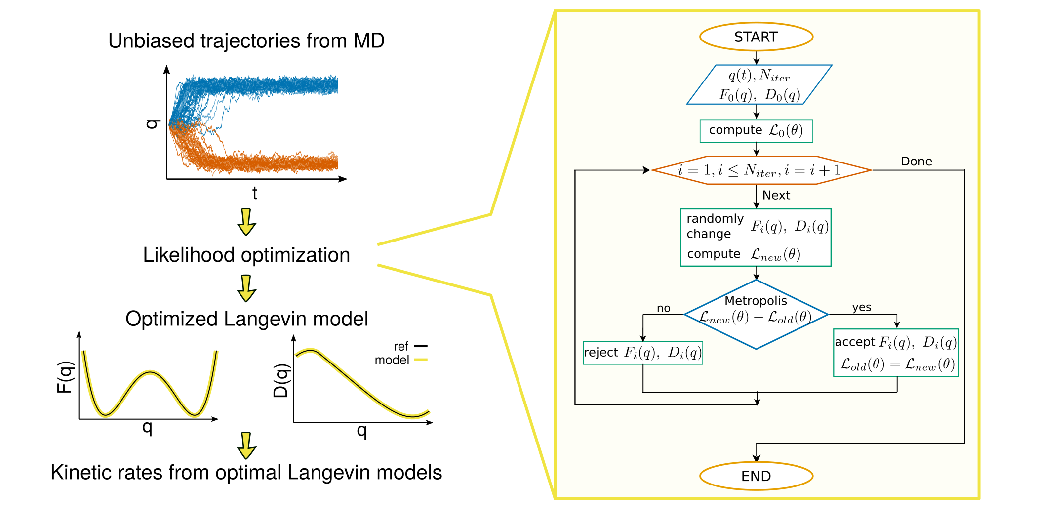
Figure 1: Schematic illustration of the approach proposed to optimize Langevin models of projected dynamics. The input data are formed by unbiased MD trajectories projected on a selected collective variable, $q(t)$. A likelihood function $\mathcal{L}(\theta)$ is maximized (i.e., $-\log\mathcal{L}(\theta)$ is minimized) by randomly varying the parameters encoding the free energy $F(q)$ and diffusion profile $D(q)$ of an overdamped Langevin equation, until optimally modeling the original MD data. At each iteration, the new parameters are accepted or rejected according to a Metropolis criterion. The optimal Langevin model corresponds to the last accepted $F(q)$ and $D(q)$ profiles, and is used for further estimation of kinetic rates (see Methods for details).

The algorithm we propose for the optimization of the likelihood function (Figure 1) is straightforward:

1. Start with trajectories $q(t)$ from MD and with an initial guess for the free energy and diffusion profiles.

2. Compute $-\log\mathcal{L}(\theta)$ for the initial data.

3. Make a random change of the free energy and diffusion profiles and compute the new $-\log\mathcal{L}(\theta)$.

4. Use a Metropolis criterion to accept or reject the new parameters.

5. Repeat $N_{\mathrm{iter}}$ times the procedure.

Note that alternatives to stochastic Monte Carlo optimization could be used; however, we appreciate the simplicity and generality of this approach, that does not require estimation of the derivatives $\partial\mathcal{L}/\partial\theta$. In all cases, we set $N_{\mathrm{iter}}=10^{6}$.

The initial guess of the parameters can facilitate the optimization of the likelihood function: without requiring any additional data besides the projected MD trajectories, an approximate value of $D$ in a free-energy minimum can be estimated from the variance of $q$ divided by its autocorrelation time ²². As sketched in Figure 1 the input trajectories $q(t)$ typically contain a final part fluctuating in the bottom of a well, that can be employed in the latter formula. The profile $D(q)$ is simply set equal to the constant estimated value. As for the initial $F(q)$, we found that the specific form is largely irrelevant. For the sake of simplicity we start from a flat profile $F(q)=0$.

The code and input files are freely available on GitHub (https://github.com/physix-repo/optLE).

B. Integration of the Langevin Equation of Motion

To generate input data for the benchmark systems, as well as to test the quality of the approximate propagator used in the likelihood function (see previous section), we numerically integrate Langevin trajectories using the Milstein algorithm, an order 1 strong Taylor scheme superior to Euler-Maruyama in the case of multiplicative noise (i.e., position-dependent diffusion): ⁴⁹

$$\begin{split}\Delta q=&\left[-\beta D(q)F^{\prime}(q)+\frac{1}{2}D^{\prime}(q)\right]\Delta t\\ &+\sqrt{2D(q)\Delta t}\,G+\frac{1}{2}D^{\prime}(q)\Delta t\,G^{2}\end{split}$$ (8)

where $G$ is a Gaussian-distributed random number with zero mean and unit variance. The integration time step $\Delta t$ is chosen after testing the observed long-time histogram of $q$ against $e^{-\beta F(q)}$, where $F(q)$ is the exact landscape used in the Langevin equation.

C. Optimal Time Resolution of the Reduced Model

The accuracy of the optimized Langevin model with respect to the original MD trajectory $q(t)$ crucially depends on the time resolution $\tau$ adopted, $q(t)\equiv q(k\tau),k=1,...,N$. In fact, it is expected that only for a sufficiently large $\tau$ the overdamped equation can model accurately the MD data. To guide the choice of $\tau$ we introduce diagnostics able to predict what choices lead to accurate models.

In general, for given profiles $F(q)$ and $D(q)$, a numerical Langevin integrator can be “inverted” to estimate the value of an effective noise $G(t)$ corresponding to each observed displacement $\Delta q=q(t+\tau)-q(t)$ in the input MD trajectory. The simplest formula corresponds to the Euler-Maruyama integrator:

$$G=\frac{\Delta q+(\beta DF^{\prime}-D^{\prime})\tau}{\sqrt{2D\tau}}$$ (9)

Another option is to invert the Milstein integrator, eq 8:

$$G=\frac{1}{D^{\prime}\tau}\Bigg{(}-\sqrt{2D\tau}+\sqrt{(2D\tau)-(2D^{\prime}\tau)\bigg{(}\frac{1}{2}D^{\prime}\tau-\beta DF^{\prime}\tau-\Delta q\bigg{)}}\Bigg{)}$$ (10)

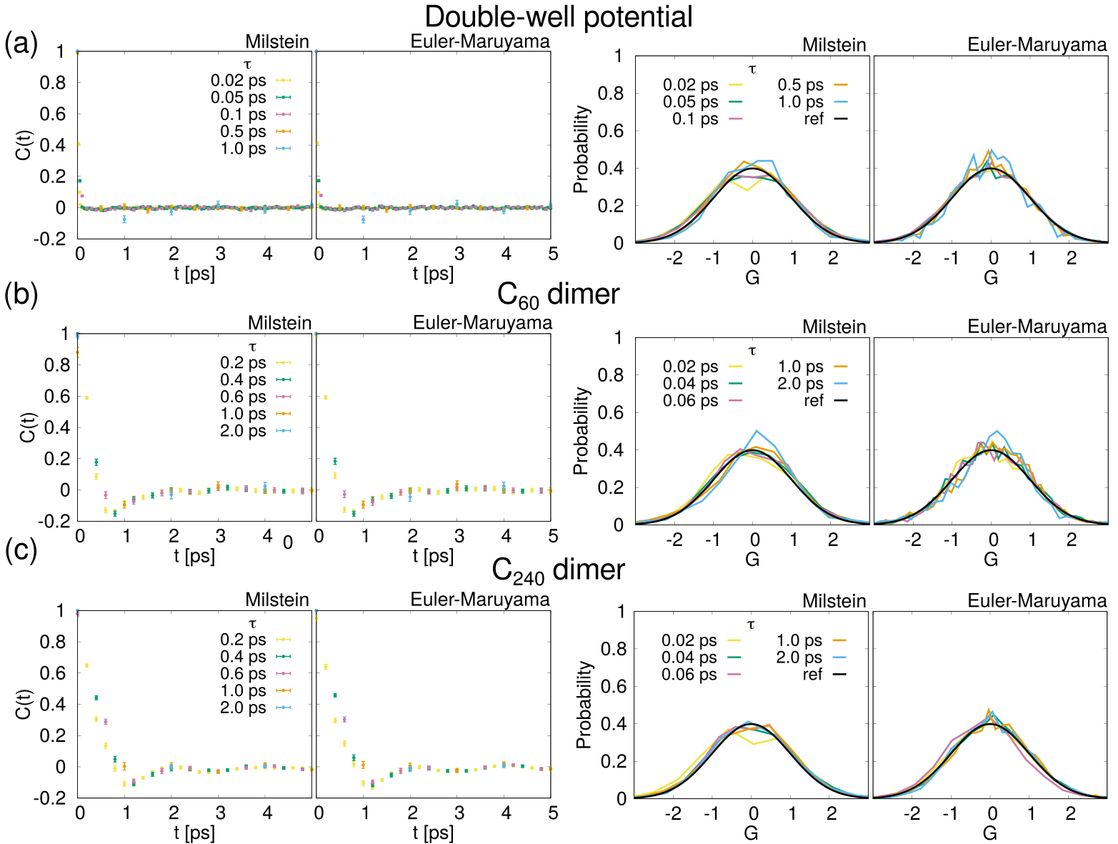
Figure S1: Autocorrelation function $C(t)$ (left panels) and distribution of the effective noise $G$ (right panels) for optimal Langevin models of different systems. The expression used to estimate the noise is found inverting the Euler-Maruyama, or the Milstein integrator, see the Methods section C, in the Main Text. (a) Symmetric double-well potential (non-overdamped input trajectories) with 10 $k_{B}T$ barrier and diffusion coefficient $0.01\leq D(q)\leq 0.02$ ps^-1 (see Fig. S3 and Fig. 2 in the Main Text). (b) C₆₀ fullerene dimer in solution. (c) C₂₄₀ fullerene dimer in solution. The different time resolutions $\tau$ used to optimize the overdamped Langevin models are shown in colors. The expected zero-mean, unit-variance Gaussian distribution of the noise is shown in black lines on the right panels. Error bars correspond to standard error over all the trajectories data-points.

If the resulting effective noise would have been generated by the model, the $G(t)$ trajectory would be random, with zero mean, unit variance and no time correlation: $\langle G(t)G(t^{\prime})\rangle=\delta_{t,t^{\prime}}$ (the latter symbol indicating the Kronecker delta, since time is discretized). Therefore, to estimate the expected accuracy of the optimal Langevin model it is possible to inspect the mean, variance, and correlation time $\tau_{\mathrm{noise}}$ of the effective noise ^{27, 40}. For the latter quantity, we adopt here a simple operative definition, as the first time where the autocorrelation function $C(t)=\langle G(0)G(t)\rangle/\langle G^{2}\rangle$ drops below 1/100. Note that in case of oscillatory behavior of $C(t)$ it is important to inspect the latter to assess if the estimate is acceptable. We find that the expressions for the noise from Euler-Maruyama (eq 9) or Milstein (eq 10) integrators yield similar results (see Supporting Information Figure S1).

As a second metric to diagnose problems in model accuracy we generate (using the integrator eq 8) $M=100$ Langevin trajectories of duration $\tau$ and time step $\Delta t\ll\tau$ starting from each point of the input trajectory $\{q_{i}\}_{i=1,...,N}$. The resulting final displacements $\tilde{q}_{i+1}^{k}-q_{i}$ (with $k=1,...,M$) are shifted and scaled according to the theoretical propagator of the model, eq 4, by subtracting $\phi_{i}$ and dividing by $\sqrt{\mu_{i}}$. In this way, their distribution would be Gaussian with zero mean and unit variance if the propagator was exact, and an average likelihood can be evaluated to estimate deviations from such ideal behavior:

$$-\overline{\log\mathcal{L}_{\mathrm{prop}}}=\frac{1}{N-1}\sum_{i=1}^{N-1}\frac{1}{M}\sum_{k=1}^{M}\frac{1}{2}\left[\log 2\pi+\left(\frac{\tilde{q}_{i+1}^{k}-q_{i}-\phi_{i}}{\sqrt{\mu_{i}}}\right)^{2}\right]$$ (11)

which yields $\frac{1}{2}[\log 2\pi+1]\approx 1.419$ in the ideal case. For increasing $\tau$, the propagator becomes unreliable, reducing the likelihood and hence allowing to predict, once again, the quality of the model (see Figure 2, 5).

D. Kinetic Rates

In general cases, the kinetic rate for a transition A$\rightarrow$B can be computed by means of the reactive flux (Bennett-Chandler) technique, that includes recrossing effects beyond transition state theory ⁵⁰

$$k(t)=\frac{\langle\dot{q}(0)\,\delta[q(0)-q^{*}]\,h_{B}[q(t)]\rangle}{\langle h_{A}\rangle}$$

where $h_{A}(q)$ and $h_{B}(q)$ are the indicator functions of metastable states $A$ and $B$. Under the hypothesis of rare transition events, there is a plateau in the values of $k$ for a broad interval of $t$ values larger than the typical microscopic time scale (e.g., of molecular vibrations) and smaller than the MFPT. $q^{*}$ is any point close to the separatrix: only efficiency is affected if they differ significantly.

The rate can be computed numerically by shooting $N_{s}$ MD simulations from $q^{*}$ with random atomic velocities drawn for the Maxwell-Boltzmann distribution: for a given $t$, $k(t)$ is the product of the sum of initial velocities for trajectories ending up in $B$, divided by the total number of shots $N_{s}$, and of a term containing information about the free energy barrier

$$k(t)=\frac{\sum_{j=1}^{N_{s}}\dot{q}_{j}(0)h_{B}[q_{j}(t)]}{N_{s}}\frac{e^{-\beta F(q^{*})}}{\int_{\Omega_{A}}dq\,e^{-\beta F(q)}}$$ (12)

We remark that for rare transitions with overdamped one-dimensional dynamics it is also possible to compute the MFPT (the inverse of the rate) as an integral over the free energy and diffusion landscapes:

$$k^{-1}(q_{0})=\int_{q_{0}}^{b}\mathrm{d}y\frac{\mathrm{e}^{\beta F(y)}}{D(y)}\int_{a}^{y}\mathrm{d}ze^{-\beta F(z)}$$ (13)

where, in the typical case of the escape from a well (even though the formula is general), $q_{0}$ is the initial position in the well, $a$ is the position of a reflective boundary located on the opposite side as the transition barrier, and $b$ is the position of an absorbing boundary located beyond the barrier. ⁵⁰ In the following, we adopt as location of the absorbing boundary $b$ the first minimum in ($\frac{\mathrm{d}}{dq})k^{-1}$ beyond the free energy barrier.

E. Molecular Dynamics Simulations

Fullerene C₆₀ Dimer

We performed MD simulations to study the interaction between two fullerene C₆₀ molecules solvated by 2398 water molecules, in a simulation box of $3.607\times 3.607\times 3.607$ nm³ with periodic boundary conditions. The initial fullerene coordinates and topology are taken from ref. 51. MD simulations are carried out using GROMACS v2019.4 ^{52, 53} patched with PLUMED 2.5.3 ⁵⁴. We adopted the SPC water model ⁵⁵ and the OPLS-AA force-field ⁵⁶ for carbon. Geometry minimization exploited the steepest descent algorithm, stopped when the maximum force was $\leq$ 50 kJ/mol$\cdot$nm. We used the leapfrog algorithm to propagate the equations of motion and the nonbonding interactions were calculated using a PME scheme with a 1.2 nm cutoff for the part in real space. We performed a 100 ps equilibration in an NVT ensemble with a stochastic velocity rescaling scheme ⁵⁷ followed by a 100 ps equilibration in an NPT ensemble using the Parrinello-Rahman barostat ⁵⁸ with a time step of 1 fs. We generated MD production trajectories without restrains, with a time step of 1 fs in the NPT ensemble at 298 K and 1 atm. The reference free-energy profile of the association/dissociation of the fullerene C₆₀ dimer in water as a function of the distance between the centers of mass $(d)$ was computed from five unbiased simulations of 500 ns each, from the population histogram: $F(d)=-k_{B}T\log\rho_{\mathrm{eq}}(q)$. We estimated the standard deviation of each histogram bin using the five simulations. The resulting profile is consistent with the free-energy profile in ref. 51.

The diffusion profile used for comparison was computed from umbrella sampling simulations in which we restrict $d$ with a harmonic potential around a reference value $d_{i}$ over different windows $i$,

$$U(d;d_{i})=\frac{c}{2}(d-d_{i})^{2}$$ (14)

Then, the diffusion coefficient in the window $i$ is estimated as the ratio between the variance of the variable ($\sigma_{d_{i}}^{2}$) and the autocorrelation time of the variable itself ($\tau^{\mathrm{corr}}$):²²

$$D(d_{i})=\frac{\sigma_{i}^{2}}{\tau^{\mathrm{corr}}_{i}}$$ (15)

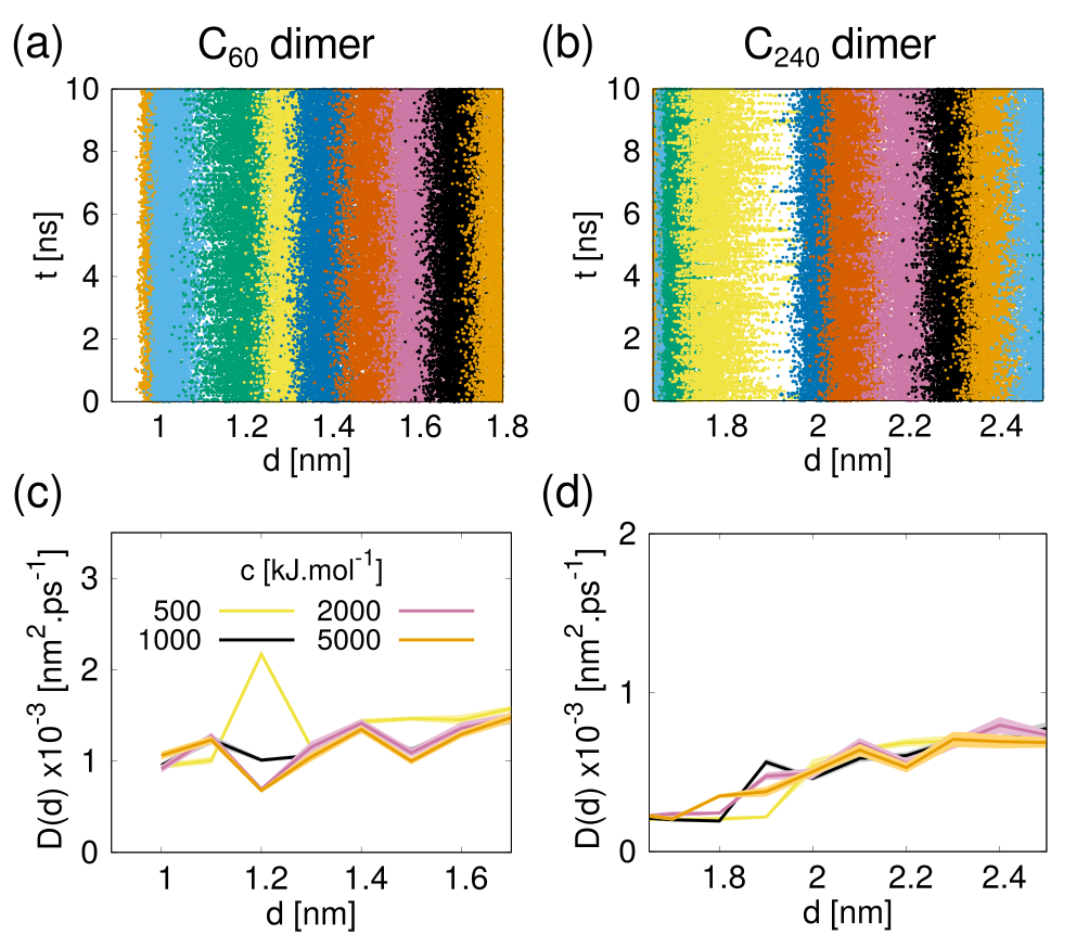
Figure S2: Diffusion profiles from umbrella sampling. Trajectory on each window for (a) C₆₀ fullerene dimer and (b) C₂₄₀ fullerene dimer using a spring constant $c=1000~{}\mathrm{kJ\cdot mol^{-1}}$. Note that for the calculation of the diffusion coefficient we do not required converged umbrella sampling calculations. Diffusion profiles $D(d)$ for different values of the spring constant $c$ for (c) C₆₀ fullerene dimer and (d) C₂₄₀ fullerene dimer.

We setup a window every 0.1 nm in a range of $d$ between 1.0 and 1.8 nm. We performed a 1 ns MD simulation for equilibration and 10 ns MD simulation production in each window with a spring constant $c=1000~{}\frac{\mathrm{kJ}}{\mathrm{mol}}$. For each window, we split the 10 ns MD simulations in 10 independent blocks of 1 ns each. We estimated the variance of $d$ and the autocorrelation time in each block. Finally, we report the average $D(d_{i})$ value and its standard error over the blocks. We note that $D(d)$ does not show large fluctuations with respect to the choice of $c$ (see Figure S2).

To generate the input trajectories for the construction of Langevin models, we employed aimless-shooting (AS) ^{59, 60} simulations. We obtained a first reactive trajectory by shooting from randomly-picked configurations of the unbiased trajectories with $d$ between 1.2 and 1.3 nm. We then performed AS using a separation $\delta t=0.1$ ps between successive shooting points, and a total length of 20 ps for each trajectory. We obtained a total of 1110 accepted trajectories relaxing from the transition state region (see Figure 3b) with an acceptance rate of 14%. The script we developed to perform AS with GROMACS is publicly available at https://github.com/physix-repo/aimless-shooting.

To estimate the dissociation rate we use the reactive flux formalism over 1000 aimless shooting trajectories. We define the dissociated state as $d\geq 1.34$ nm and the associated state as $d\leq 1.17$ nm (see Figure 3a). The value of the MFPT obtained with reactive flux was validated with the brute force estimate from 100 unbiased MD trajectories launched from the bound state: $6.1\pm 1.2$ ns versus $6.5\pm 0.6$ ns, respectively. Finally, we estimated the transmission coefficient as ⁵⁰

$$\kappa=\frac{k_{A\rightarrow B}^{RF}}{k_{A\rightarrow B}^{TST}}~{},$$ (16)

where $k_{A\rightarrow B}^{RF}$ is the dissociation rate constant from reactive flux (eq 12), and $k_{A\rightarrow B}^{TST}$ is the dissociation rate constant from transition state theory. The estimated transmission coefficient for the dissociation of the fullerene C₆₀ dimer is 0.37, meaning that the number of recrossings before relaxation is small.

Fullerene C₂₄₀ Dimer

We also simulated the interaction between bigger fullerenes, featuring a more stable complex: two C₂₄₀ molecules in water solution. We used the structure of the fullerene molecule from ref. 61. We built the topology automatically using the OBGMX web server ⁶², solvating the fullerenes with 5375 water molecules in a simulation box of $5.22\times 5.22\times 5.22$ nm³, conserving the same parameters for the Lennard-Jones potentials used in the simulation of the C₆₀ fullerenes. The parameters of the MD simulations also remain the same as for C₆₀.

Given the stability of the bound state, to estimate the reference free energy profile we used well-tempered metadynamics simulations ⁶³, adding bias over the distance between the center of mass ($d$) with an initial Gaussian height of 1.0 kJ/mol and width of 0.01 nm. The bias factor was set to 8, and Gaussians were deposited every 1 ps. Five replicas of 500 ns each were simulated. We estimate the reference free energy profile and its statistical uncertainty from the average and standard deviation of the free energy profiles from all simulations. We obtained the diffusion profiles for comparison from umbrella sampling simulations following the same procedure and with the same parameters used for C₆₀ fullerene dimer. We placed a window every 0.1 nm in a range of $d$ from 1.6 to 2.6 nm. We performed AS simulations following the same procedure used for C₆₀ fullerenes. We obtained 1515 accepted trajectories of 100 ps each, with an acceptance rate of 15%. We calculate the dissociation rate using 1000 trajectories and reactive flux: $9.4\pm 1.1$ $\mu$s. We define the dissociated state as $d\geq 2.01$ nm and the associated state as $d\leq 1.9$ nm. The estimated transmission coefficient is 0.6.

Results and Discussion

In the new approach, the Langevin model is parametrized from unbiased MD trajectories spanning the relevant CV region. Such trajectories can be easily obtained as spontaneous out-of-equilibrium relaxation from initial high free-energy configurations, e.g., the top of a barrier. Several effective techniques are available to discover transition states and reactive paths at a moderate computational cost ^{64, 44, 65, 66, 67, 68}: although not trivial, this task is generally much less involved than reconstructing accurate free energy profiles. In the following we use as input CV-projected MD trajectories $q(t)$ obtained from TPS or by shootings from the barrier top and relaxing into the minima. Note that such trajectories are short, since in rare events the transition path time is typically very fast compared to the waiting time in a minimum, that is, the MFPT.

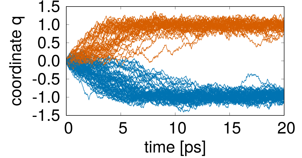
Figure S3: 100 input trajectories generated with a non-overdamped Langevin integrator, using the standard Langevin equation: $\dot{p}=-\frac{\partial F(q)}{\partial q}-\gamma p+\sqrt{2k_{B}Tm\gamma}\,\eta(t)$. The benchmark system is a symmetric double-well free-energy landscape with 10 $k_{B}T$ barrier ($m=1~{}k_{B}T~{}\cdot$ ps^-2). 53% of the trajectories ended up in the right basin and 47% in the left basin.

As an initial benchmark we verify whether our method yields Langevin models accurately reproducing the correct $F(q)$ and $D(q)$ starting from underdamped Langevin trajectories. The input data are composed by 100 short underdamped Langevin trajectories $q(t)$, each one 20 ps long, relaxing from the barrier top of a double-well landscape (see Supplementary Figure S3). The exact free energy and diffusion profiles are shown in black in Figure 2.

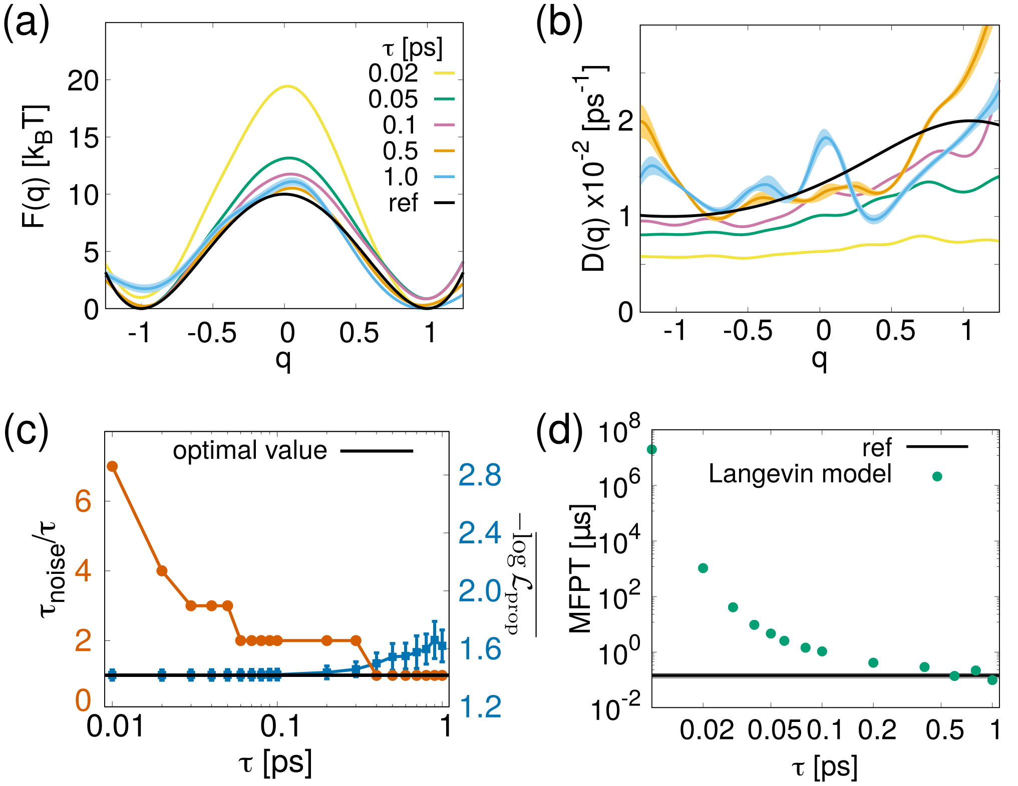
Figure 2: Optimal overdamped Langevin models (eq 1) for different resolutions $\tau$ starting from underdamped trajectories on a double-well free-energy landscape. (a) $F(q)$ and (b) $D(q)$ profiles (exact ones are shown with black lines); vertical bars correspond to standard error over 10 independent stochastic optimizations. (c) Autocorrelation time of the effective noise $\tau_{\mathrm{noise}}$ (eq 10) normalized by $\tau$ (i.e., number of correlated steps), and average likelihood quantifying the accuracy of the propagator (eq 11). The black line represents the ideal values. Vertical bars are the standard deviation over all trajectory steps $\Delta q$. (d) MFPTs for the optimal overdamped Langevin models shown in panels a and b, computed with eq 13: the reference value in black is computed with reactive flux on the exact profiles in black in panels a and b. Vertical bars are the standard error over 10 independent Langevin models (hardly visible at this scale).

Since the initial trajectories are generated with an underdamped integrator, building the overdamped model entails projecting out the momentum $p$ conjugated to the CV position $q$. As a result, a $q$-based Langevin model is expected to display memory (time correlation) in the friction and noise for $\tau$ comparable to the integration time step $\Delta t=10^{-4}$ ps. Adopting coarse-enough $\tau$ resolutions, on the other hand, should lead to memory-less behavior, well reproduced by an overdamped model.

To test this hypothesis, in Figure 2 we generate Langevin models using $0.01$ ps $\leq\tau\leq 1$ ps: for the smallest $\tau$ value, the model strongly overestimates the barrier and underestimates the diffusion coefficient. As $\tau$ increases the reconstructed model becomes more accurate (see Figure 2) until at large values of $\tau$ the error increases again. We found that there is a relatively narrow range of $\tau$ values for which the Langevin overdamped model is accurate: to identify the optimal range in real-world applications we propose two complementary tests that allow identifying the upper and lower boundaries of $\tau$ bracketing the high-quality Langevin models.

The lower acceptable $\tau$ is the smallest time displaying no memory effects, measured through the autocorrelation of the effective Langevin noise, that is, the noise extracted a posteriori by analyzing the original trajectory with the optimal Langevin model, eq 10 (see Figure S1 for details). The upper limit on $\tau$ corresponds to the onset of a significant deviation between the approximate and the exact propagators (the latter estimated from accurate numerical integration, see methods section C and eq 11). Both diagnostics are reported in Figure 2c, and together they predict that the Langevin model should attain the best accuracy for $\tau$ values close to 0.5 ps: large enough to avoid memory, but small enough for the short-time propagator to remain reliable.

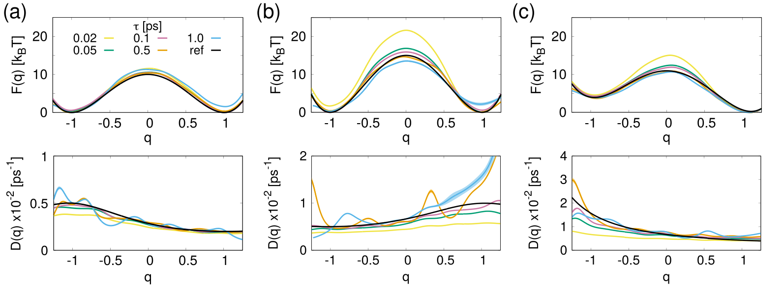
Figure S4: Optimal overdamped Langevin models, each one trained on 100 non-overdamped Langevin trajectories of 50 ps relaxing from the barrier top. (a) Symmetric double-well potential with 10 $k_{B}T$ barrier and diffusion coefficient $0.002\leq D(q)\leq 0.005$ ps^-1. (b) Symmetric double-well potential with 15 $k_{B}T$ barrier and diffusion coefficient $0.005\leq D(q)\leq 0.01$ ps^-1. (c) Asymmetric double-well potential with 10 $k_{B}T$ barrier and diffusion coefficient $0.005\leq D(q)\leq 0.03$ ps^-1. The different time resolutions $\tau$ employed to optimize the models are shown in colors. The exact profiles are shown with black lines. The thickness of the lines correspond to standard error over 10 independent stochastic optimization runs.

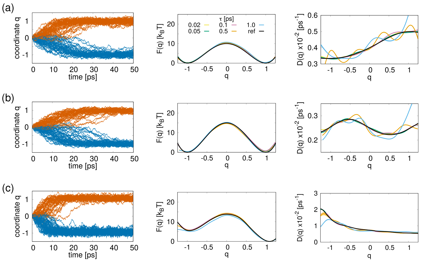
Figure S5: Optimal overdamped Langevin models trained on overdamped Langevin trajectories. (a) Symmetric double-well potential with 10 $k_{B}T$ barrier and diffusion coefficient $0.003\leq D(q)\leq 0.005$ ps^-1. (b) Symmetric double-well potential with 15 $k_{B}T$ barrier and diffusion coefficient $0.0022\leq D(q)\leq 0.0028$ ps^-1. (c) Asymmetric double-well potential with 13 $k_{B}T$ barrier and diffusion coefficient $0.005\leq D(q)\leq 0.025$ ps^-1. Left: 100 input trajectories of 50 ps obtained with an overdamped integrator, Eq. 8 in the Main Text, relaxing from the barrier top. Center: optimal free energy profiles. Right: optimal diffusion profiles. The different time resolutions $\tau$ employed to optimize the models are shown in colors. The exact profiles are shown with black lines. The thickness of the lines correspond to standard error over 10 independent stochastic optimization runs.

Overall, when selecting $\tau$ based on the proposed diagnostics, models converge smoothly and rapidly ($<10^{6}$ Monte Carlo steps) to a good approximation of the exact results: as few as 100 reference trajectories are sufficient to reconstruct the free energy profile to within 1 $k_{B}T$ and $D(q)$ to within 15% error (we remark that fluctuations in $D(q)$ appear converged with respect to the different parameters used in the reconstruction of the models and irrespective of the input trajectories). The same conclusions can be derived regardless of the shape of the diffusion and free energy profiles (see Figure S4). We remark that, when the input trajectories are generated with an overdamped integrator, the reconstructed profiles deviate less than 1 $k_{B}T$ and 10%, respectively, from the exact $F(q)$ and $D(q)$, regardless of $\tau$, unless when it is too large for our approximate propagator (see Figure S5).

Besides estimating free energy and diffusion profiles, a key objective of the new method is the accurate prediction of kinetic rates at a moderate computational cost. Figure 2d shows the MFPTs obtained with eq 13 using the optimal Langevin models. Too small values of $\tau$ lead to strongly overestimated MFPT, as expected from the overestimated barriers, while the rate becomes accurate for $\tau$ values within the predicted optimal window (Figure 2c). On the other hand, for $\tau$ larger than optimal, MFPTs in the same order of magnitude as the reference value are still obtained.

We note that, alternatively, we can compute the MFPT using the reactive flux technique ^{69, 70}, free from transition state approximations.  This traditionally requires two distinct sets of expensive simulations, one to compute the free energy barrier and another to compute a correlation function accounting for recrossings (see methods section D and Table S1). However, this technique becomes inexpensive if combined with our approach, since the free energy barrier is directly obtained from likelihood optimization on short trajectories, while recrossing statistics can be accurately estimated from inexpensive synthetic Langevin trajectories. We remark that the rates computed from eq 13 are similar to those of reactive flux (see Table S2).

The double-well potentials in the previous section allowed us to benchmark the scope and limitations of the method while having full control over the system. To assess the method in realistic complex systems, we modeled the dynamics of two fullerene molecules in explicit water, considering two different sizes C₆₀ and C₂₄₀ (Figure 3). The free-energy landscape as a function of the distance $d$ between fullerenes’ centers of mass features a minimum for the bound complex (with different depth for the two sizes) and a relatively flat region for the dissociated state, see black lines in Figure 4. The resulting rare dissociation events and diffusion-controlled association events ^{71, 72, 73, 51} are analogous to other processes such as protein-protein interaction. We obtained reference free-energy profiles using 2.5 $\mu$s-long brute-force MD trajectories for the C₆₀ dimer, while we employed well-tempered metadynamics ⁶³ for the C₂₄₀ dimer due to its very low dissociation rate. The diffusion profiles are obtained from sets of 10 ns umbrella sampling simulations every 0.1 nm in distance between the center of mass (see methods section E for details).

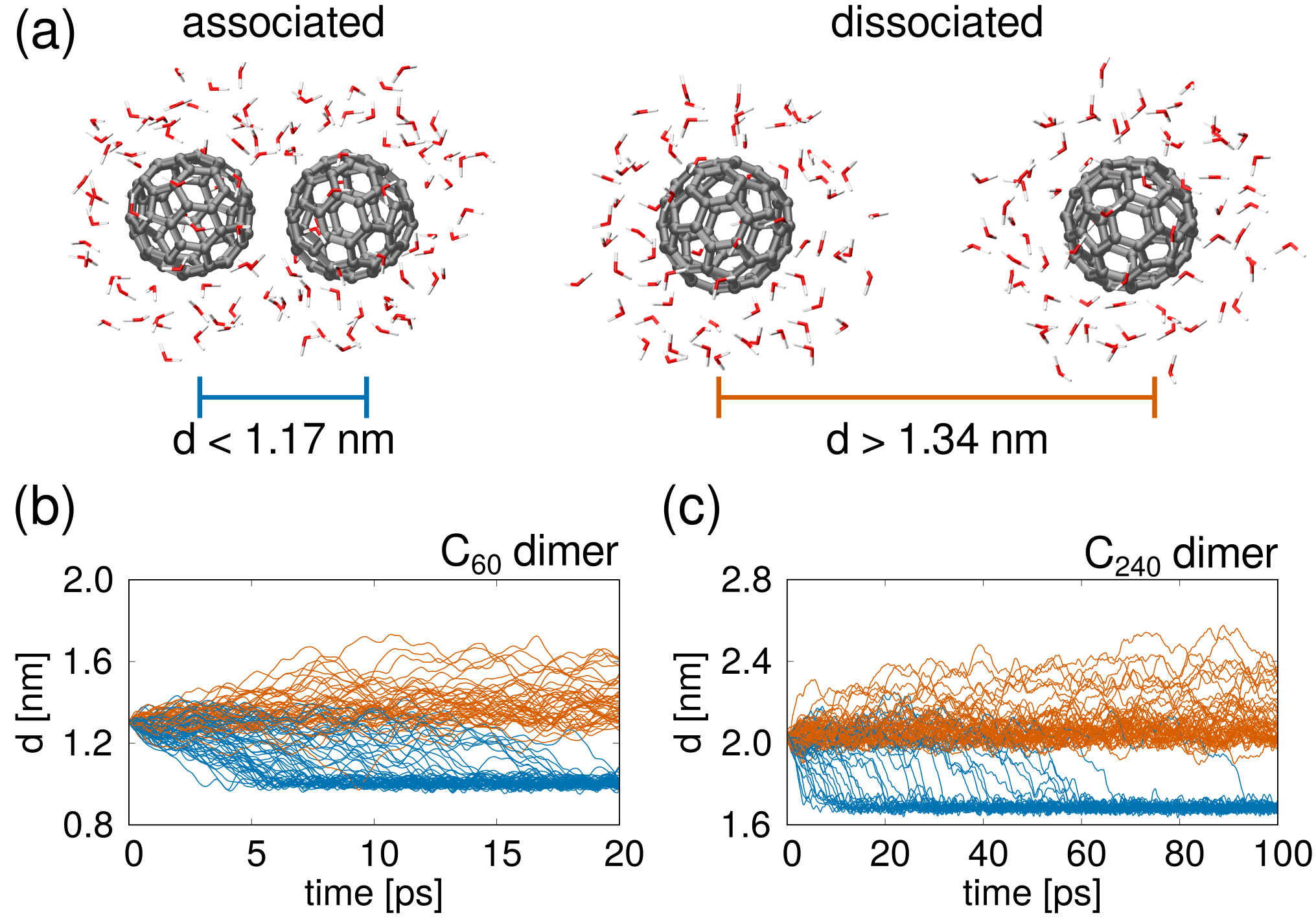
Figure 3: (a) Characteristic atomic configurations for the C₆₀ dimer in bulk water solution; only waters distant less than 5 Å from carbon atoms are shown. The associated and dissociated states are defined in terms of the distance $d$ between the centers of mass of the fullerenes. (b) 100 MD trajectories (from aimless shooting) starting from the transition state ensemble and featuring the association (blue) or dissociation (orange) of the C₆₀ dimer, and (c) of the C₂₄₀ dimer, respectively.

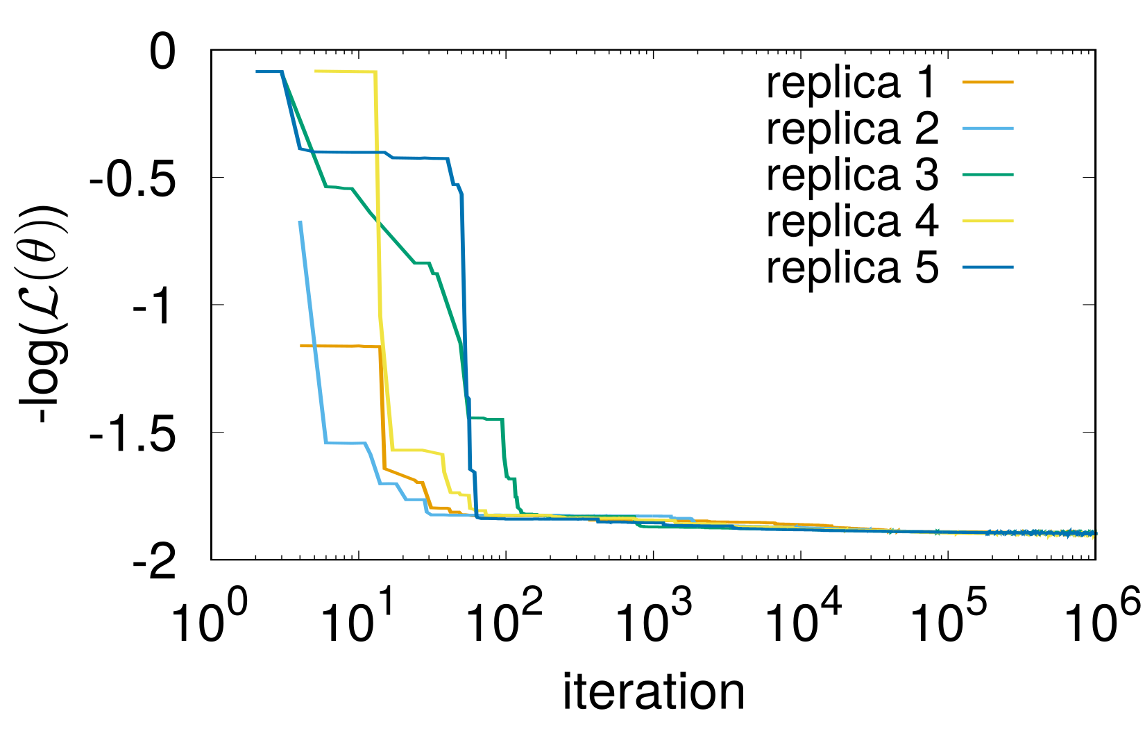
Figure S6: Example of the convergence of $-\log\mathcal{L}(\theta)$ as a function of the number of iterations for the C₆₀ fullerene dimer in solution. Colors represent different independent optimizations. A similar behavior with a smooth convergence is observed in all the Langevin models presented in this work.

We maximized the likelihood of Langevin models starting from short aimless shooting ⁵⁹ TPS trajectories (20/100 ps each, cumulative duration 2/10 ns for C₆₀/C₂₄₀, see Figure 3). An example of the convergence of $-\log\mathcal{L}(\theta)$ as a function of the number of iterations is shown in Figure S6. We adopted a range of time resolutions $\tau$ between 0.1 and 2 ps: for fast time scales, memory is expected to arise from the projection of the solvated fullerenes many-body dynamics on a single CV. Sizable memory effects are evident in the effective noise (eq 10) for $\tau<0.5$ ps (see also Figure S1), severely affecting the accuracy of $F(d)$. For larger $\tau$ values, similarly to the case of the analytic double-well potential, the Langevin models become increasingly accurate: memory decays after about 0.5 ps for the smaller fullerenes and after about 1.0 ps for the bigger ones. As for the diffusion profile, all models show $D(d)$ in the same order of magnitude, in good agreement with the diffusion coefficients estimated from umbrella sampling ²² (see methods section E). We remark that generating 100 short TPS trajectories for Langevin optimization can be computationally faster than generating a sufficient amount of umbrella sampling trajectories to estimate the diffusion profile.

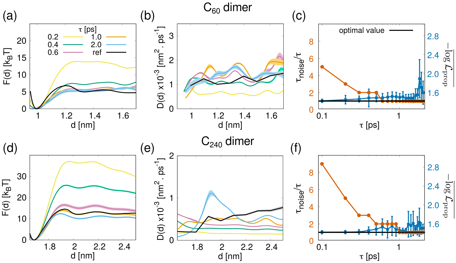
Figure 4: Optimal Langevin models for the interaction of C₆₀ and C₂₄₀ fullerene dimers in explicit water, for different values of the time resolution $\tau$. The input data set consists of 100 MD trajectories (aimless shooting) relaxing from the transition state ensemble in Figure 3. (a, d) Free-energy profiles $F(q)$, compared to the reference ones in black: vertical bars correspond to standard deviations over 10 independent stochastic optimizations. (b, e) Diffusion profiles $D(q)$, compared to the umbrella sampling ones in black: vertical bars correspond to standard deviations over 10 independent stochastic optimizations. (c, f) Autocorrelation time of the effective noise (eq 10) normalized by $\tau$ (i.e., number of correlated steps), and average likelihood quantifying the accuracy of the propagator (eq 11). The black line represents the ideal value for both quantities; vertical bars refer to the standard deviation over all trajectory steps $\Delta q$.

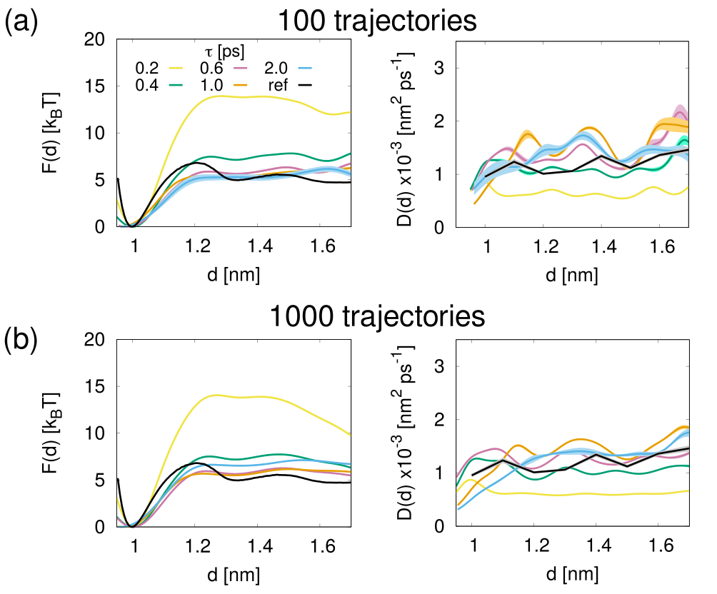
Figure S7: Effect of the number of input trajectories. Optimal free energy and diffusion profiles reconstructed from (a) 100 and (b) 1000 initial MD trajectories of 20 ps for the C₆₀ fullerene dimer. The different time resolutions $\tau$ employed to optimize the models are shown in colors. The reference free energy profile (computed from brute force MD) and diffusion profile (computed from umbrella sampling) are shown with black lines. The thickness of the lines correspond to standard error over 10 independent optimization runs.

On the other hand, the quality of the approximate short-time propagator eq 6 decreases as $\tau$ increases. Accurate results are clearly identified in the range of $\tau$ that minimizes both non-Markovian behavior and error propagation (see Figure 4). Interestingly, optimizing the models based on 1000 reference trajectories instead of 100 yields minimal improvements (see Supplementary Figure S7).

Finally, we assessed the accuracy of kinetic predictions given by the models. The dissociation MFPT is on the nanosecond and microsecond scales, respectively, for C₆₀ and C₂₄₀ dimers; that is, 2 and 5 orders of magnitude slower than the out-of-equilibrium MD trajectories used for training. For each value of $\tau$, we computed MFPTs using eq 13 on the optimal models, yielding Figure 5. We emphasize that the latter approach allows computation of the MFPT without generating any additional expensive MD trajectories.

For too small values of $\tau$, the barrier is overestimated (see Figure 4), leading to overestimation of the MFPTs by several orders of magnitude. For the C₆₀ dimer the MFPT becomes accurate (compared to the brute force result) for $\tau>0.5$ ps, while for the C₂₄₀ dimer this level of accuracy requires $\tau>1$ ps: once again, these are the optimal time resolutions predicted by the diagnostics in Figure 4. Taken together, all these results demonstrate that the approximations inherent in the Langevin models are under control, leading to accurate predictions about the thermodynamics and kinetics of complex systems.

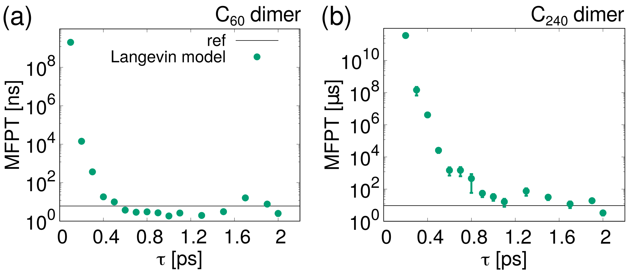
Figure 5: MFPTs computed from the optimal Langevin models generated with different time resolutions $\tau$, for the dissociation of fullerene (a) C₆₀, and (b) C₂₄₀ dimer, in water solution. MFPTs are estimated from eq 13 (reference value in black). Vertical bars are the standard error over 10 independent Langevin models.

Concluding Remarks

The calculation of free energy landscapes and kinetic rates is key tasks of computer simulations of complex systems. Even though these two tasks are usually tackled using different ad hoc techniques,² the main contribution of the present work consists in demonstrating that they can be simultaneously achieved in a conceptually simple way, by estimating Langevin models starting from a relatively inexpensive set of about one hundred TPS-like trajectories, regardless of the barrier height. Likelihood maximization – an efficient parameter estimation technique – is combined with a double test bracketing the time resolution $\tau$, granting control over the accuracy of the model. The choice of a suitable $\tau$ is especially important for accurately estimating the free energy, because the rate has an exponential dependence on the barrier while only having a linear dependence on $D$.

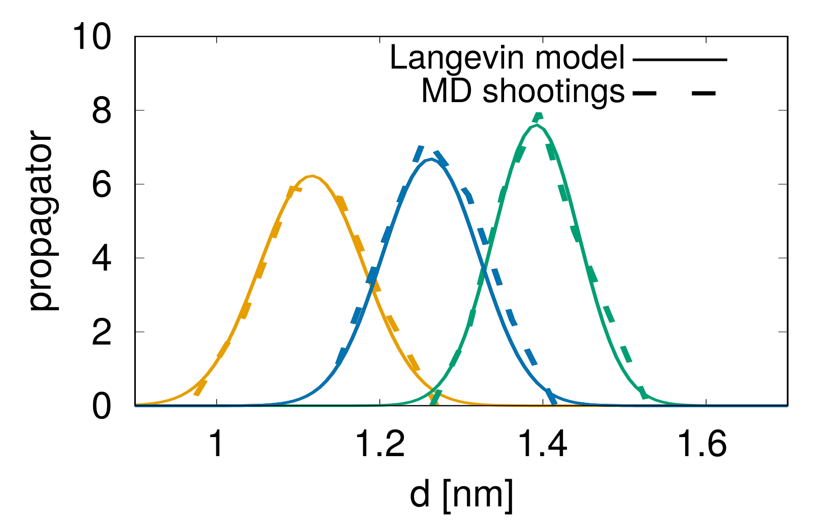
Figure S8: Propagator test. Comparison between $p(q^{\prime},t+\tau|q,t)$ predicted by the optimal Langevin model and a distribution of MD shootings trajectories for the C₆₀ fullerene dimer. The time resolution was set to $\tau=1$ ps. The optimized free energy and diffusion profiles (Fig. 4.a. Main Text, orange profiles) were used to estimate the short time transition probability (eq. 4. in the Main Text) predicted by the Langevin model (solid lines). The distribution from MD correspond to the histograms of the displacement after 1 ps from sets of 500 shooting trajectories (dashed lines). We use 5 shooting points extracted from a long unbiased trajectory for each location: before the barrier (orange), at the barrier top (blue), and after the barrier (green).

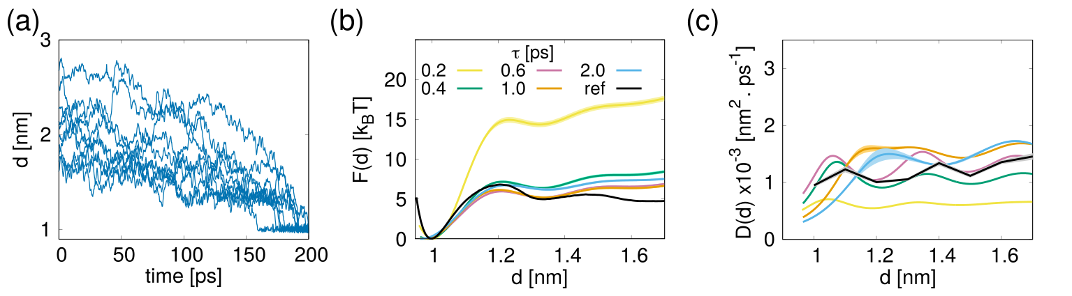
Figure S9: Langevin models from association trajectories. (a) Examples of 100 association trajectories used to optimized the (b) free energy and (c) diffusion profiles from 200 ps MD trajectories of the C₆₀ fullerene dimer. The different time resolutions $\tau$ employed to optimize the models are shown in colors. The reference free energy profile (computed from brute force MD) and diffusion profile (computed from umbrella sampling) are shown with black lines. The thickness of the lines correspond to standard error over 10 independent optimization runs.

The resulting Markovian Langevin equations reproduce well the quantitative thermodynamic and dynamic properties of the original many-body system, including accurate kinetic rates, despite a gap of many orders of magnitude with respect to the short MD trajectories used for training. Moreover, the short time transition probability $p(q^{\prime},t+\tau|q,t)$ predicted by the optimal Langevin model (eq 4) is in good agreement with a distribution collected from short MD shootings of length $\tau$ (see example in Figure S8). Incidentally, we note that our approach is not restricted to transition path sampling: in principle, any set of unbiased trajectories spanning the regions of interest could be used to train the Langevin model (see example in Figure S9).

We also remark that equilibrium properties are systematically recovered from out-of-equilibrium data: standard transition path sampling trajectories are the golden standard for the study of transformation mechanisms, however, since such data set is a small subset of all possible (reactive and nonreactive) pathways, lacking Boltzmann distribution of the configurations, it cannot be used for the direct estimate of equilibrium histograms (i.e., free energies) and rate matrices (e.g., in Markov state models) by simple averaging ^{74, 4}. Here we show that the contrary is true, provided bare transition paths are employed to train a suitable stochastic model (see also refs. 21, 75, 22, 29, 76, 77 for related or alternative ideas). Note that Langevin equations of motion, compared to other machine-learning tools, retain a direct physical interpretation, with the separation between a systematic average force and friction/noise effects describing the projected-out degrees of freedom (commonly referred to as “the bath”).

In future applications of the new approach, two main issues have to be taken into consideration. First, different kinds of Langevin equation (generalized, standard or overdamped) can be necessary to faithfully reproduce the projected dynamics of a complex system, depending on the physical process, the choice of the CV, and the observational time scale. For chemical reactions in water the memory time scale could be comparable to the transition path time, requiring a non-Markovian equation, whereas for crystal nucleation or protein folding Markovian models are customarily invoked. In the present work, we demonstrated the approach using overdamped Langevin equations: in principle, this can be generalized to other stochastic models by replacing the propagator expression (eq 6) with a different suitable approximation, based on ideas in refs. 48, 43.

A second issue concerns the effect of projecting the dynamics on suboptimal CVs, rather than on the ideal reaction coordinate, commonly identified with the committor function ^{15, 78, 79}. In principle, the CV definition can be systematically optimized with an iterative scheme, in which a single initial set of MD trajectories can be employed to build optimal Langevin models for progressively improving CVs. A related idea was recently proposed in the case of discrete Markov state models ^{80, 81}. Therefore, our new approach represents a starting point both for the systematic modeling of MD data through physically-motivated stochastic equations as well as for machine-learning approaches to reaction coordinate optimization.

Supporting information

The Supporting Information is available free of charge at https://pubs.acs.org/doi/10.1021/acs.jctc.2c00324. Detailed results for different shapes of the double-well benchmark systems, autocorrelation functions of the effective noise, convergence tests, and kinetic rate estimates using reactive flux

The authors declare no competing financial interest.

Supporting Information

Supplementary Figures

Supplementary Tables

Method	N. trajs	MFPT (ns)
Brute force	100	18.2 $\pm$ 0.1
Reactive flux	1000	90 $\pm$ 69
	2000	25 $\pm$ 4
	5000	27 $\pm$ 2
	8000	20.8 $\pm$ 0.3
	10000	19.1 $\pm$ 0.1
	12000	19.07 $\pm$ 0.09
	15000	18.24 $\pm$ 0.05
	18000	18.17 $\pm$ 0.04
	20000	18.20 $\pm$ 0.07

Table S1: Brute force vs reactive flux estimate of the MFPT. We used as a benchmark system a double-well potential with a 7 $k_{B}T$ barrier and $50\leq\gamma(q)\leq 150$ ps. Brute force estimate is obtained as the average escape time of 100 trajectories (at least 50 ns-long) starting from the minimum. Reactive flux estimate is obtained with Eq. 12 in the Main Text, and different number of trajectories. Each trajectory is 40 ps-long. We note that at least 20000 trajectories are needed to converge the reactive flux estimate. We highlight that in practical applications, the need of large amount of trajectories to converge the correlation function of Eq. 12 in the Main Text restricts the use of reactive flux.

$\tau$	MFPT ($\mu$s) from Eq. 13	MFPT ($\mu$s) from eq. 12
0.02	1052 $\pm$ 51	1398 $\pm$ 11
0.05	4.6 $\pm$ 0.3	3.1 $\pm$ 0.3
0.10	1.1 $\pm$ 0.1	0.83 $\pm$ 0.02
0.50	0.27 $\pm$ 0.03	0.20 $\pm$ 0.05
1.00	0.10 $\pm$ 0.01	0.13 $\pm$ 0.01

Table S2: Comparison between MFPTs estimated from Eq. 13 in the Main Text and from reactive flux for the double-well potential in Fig. 2. The brute force estimate is $0.14\pm 0.08$ $\mu$s. The reactive flux estimate is obtained with Eq. 12 in the Main Text and 10000 trajectories, each one 20 ps-long .

References

- Pietrucci 2017 Fabio Pietrucci. Strategies for the exploration of free energy landscapes: unity in diversity and challenges ahead. Rev. Phys., 2:32–45, 2017. doi: 10.1016/j.revip.2017.05.001.
- Camilloni and Pietrucci 2018 Carlo Camilloni and Fabio Pietrucci. Advanced simulation techniques for the thermodynamic and kinetic characterization of biological systems. Adv. Phys. X, 3(1):1477531, 2018. doi: 10.1080/23746149.2018.1477531.
- Dellago and Bolhuis 2008 Christoph Dellago and Peter G Bolhuis. Transition path sampling and other advanced simulation techniques for rare events. Springer Berlin Heidelberg, 2008.
- Bolhuis and Swenson 2021 Peter G Bolhuis and David WH Swenson. Transition path sampling as markov chain monte carlo of trajectories: Recent algorithms, software, applications, and future outlook. Advanced Theory and Simulations, 4(4):2000237, 2021.
- Van Erp and Bolhuis 2005 Titus S Van Erp and Peter G Bolhuis. Elaborating transition interface sampling methods. Journal of computational Physics, 205(1):157–181, 2005.
- Allen et al. 2005 Rosalind J Allen, Patrick B Warren, and Pieter Rein Ten Wolde. Sampling rare switching events in biochemical networks. Phys. Rev. Lett., 94(1):018104, 2005.
- Zwanzig 2001 Robert Zwanzig. Nonequilibrium statistical mechanics. Oxford University Press, 2001.
- Risken 1996 Hannes Risken. The Fokker-Planck Equation. Springer, 1996.
- Łuczka 2005 J Łuczka. Non-markovian stochastic processes: Colored noise. Chaos, 15(2):026107, 2005.
- Grote and Hynes 1980 Richard F Grote and James T Hynes. The stable states picture of chemical reactions. ii. rate constants for condensed and gas phase reaction models. J. Chem. Phys., 73(6):2715–2732, 1980.
- Lee et al. 2015 Hee Sun Lee, Surl-Hee Ahn, and Eric F Darve. Building a coarse-grained model based on the mori-zwanzig formalism. MRS Online Proceedings Library Archive, 1753, 2015. doi: 10.1557/opl.2015.185.
- Daldrop et al. 2018 Jan O Daldrop, Julian Kappler, Florian N Brünig, and Roland R Netz. Butane dihedral angle dynamics in water is dominated by internal friction. Proc. Natl. Acad. Sci. U.S.A., 115(20):5169–5174, 2018.
- Van Kampen 1992 Nicolaas Godfried Van Kampen. Stochastic processes in physics and chemistry, volume 1. Elsevier, 1992.
- Coffey and Kalmykov 2012 William Coffey and Yu P Kalmykov. The Langevin equation: with applications to stochastic problems in physics, chemistry and electrical engineering. World Scientific, 2012.
- Lu and Vanden-Eijnden 2014 Jianfeng Lu and Eric Vanden-Eijnden. Exact dynamical coarse-graining without time-scale separation. The Journal of Chemical Physics, 141(4):044109, 2014. doi: 10.1063/1.4890367. URL https://doi.org/10.1063/1.4890367.
- Straub et al. 1987 John E Straub, Michal Borkovec, and Bruce J Berne. Calculation of dynamic friction on intramolecular degrees of freedom. J. Phys. Chem., 91(19):4995–4998, 1987.
- Tuckerman and Berne 1993 M Tuckerman and BJ Berne. Vibrational relaxation in simple fluids: Comparison of theory and simulation. The Journal of chemical physics, 98(9):7301–7318, 1993.
- Timmer 2000 J Timmer. Parameter estimation in nonlinear stochastic differential equations. Chaos, Solitons & Fractals, 11(15):2571–2578, 2000.
- Gradišek et al. 2000 Janez Gradišek, Silke Siegert, Rudolf Friedrich, and Igor Grabec. Analysis of time series from stochastic processes. Phys. Rev. E, 62(3):3146, 2000.
- Chorin et al. 2002 Alexandre J Chorin, Ole H Hald, and Raz Kupferman. Optimal prediction with memory. Phys. D, 166(3-4):239–257, 2002.
- Hummer and Kevrekidis 2003 Gerhard Hummer and Ioannis G Kevrekidis. Coarse molecular dynamics of a peptide fragment: Free energy, kinetics, and long-time dynamics computations. J. Chem. Phys., 118(23):10762–10773, 2003.
- Hummer 2005 Gerhard Hummer. Position-dependent diffusion coefficients and free energies from bayesian analysis of equilibrium and replica molecular dynamics simulations. New J. Phys., 7(1):34, 2005.
- Best and Hummer 2006 Robert B Best and Gerhard Hummer. Diffusive model of protein folding dynamics with kramers turnover in rate. Phys. Rev. Lett., 96(22):228104, 2006.
- Lange and Grubmüller 2006 Oliver F Lange and Helmut Grubmüller. Collective langevin dynamics of conformational motions in proteins. J. Chem. Phys., 124(21):214903, 2006.
- Horenko et al. 2007 Illia Horenko, Carsten Hartmann, Christof Schütte, and Frank Noe. Data-based parameter estimation of generalized multidimensional langevin processes. Phys. Rev. E, 76(1):016706, 2007.
- Darve et al. 2009 Eric Darve, Jose Solomon, and Amirali Kia. Computing generalized langevin equations and generalized fokker–planck equations. Proc. Natl. Acad. Sci. U.S.A., 106(27):10884–10889, 2009.
- Micheletti et al. 2008 Cristian Micheletti, Giovanni Bussi, and Alessandro Laio. Optimal langevin modeling of out-of-equilibrium molecular dynamics simulations. J. Chem. Phys., 129(7):074105, 2008.
- Berezhkovskii and Szabo 2011 Alexander Berezhkovskii and Attila Szabo. Time scale separation leads to position-dependent diffusion along a slow coordinate. The Journal of chemical physics, 135(7):074108, 2011.
- Zhang et al. 2011 Qi Zhang, Jasna Brujić, and Eric Vanden-Eijnden. Reconstructing free energy profiles from nonequilibrium relaxation trajectories. J. Stat. Phys., 144(2):344–366, 2011.
- Crommelin and Vanden-Eijnden 2011 Daan Crommelin and Eric Vanden-Eijnden. Diffusion estimation from multiscale data by operator eigenpairs. Multiscale Modeling & Simulation, 9(4):1588–1623, 2011.
- Crommelin 2012 Daan Crommelin. Estimation of space-dependent diffusions and potential landscapes from non-equilibrium data. Journal of Statistical Physics, 149(2):220–233, 2012.
- Schaudinnus et al. 2015 Norbert Schaudinnus, Björn Bastian, Rainer Hegger, and Gerhard Stock. Multidimensional langevin modeling of nonoverdamped dynamics. Phys. Rev. Lett., 115(5):050602, 2015.
- Schaudinnus et al. 2016 Norbert Schaudinnus, Benjamin Lickert, Mithun Biswas, and Gerhard Stock. Global langevin model of multidimensional biomolecular dynamics. J. Chem. Phys., 145(18):184114, 2016. doi: 10.1063/1.4967341.
- Lesnicki et al. 2016 Dominika Lesnicki, Rodolphe Vuilleumier, Antoine Carof, and Benjamin Rotenberg. Molecular hydrodynamics from memory kernels. Phys. Rev. Lett., 116(14):147804, 2016.
- Meloni et al. 2016 Roberto Meloni, Carlo Camilloni, and Guido Tiana. Properties of low-dimensional collective variables in the molecular dynamics of biopolymers. Phys. Rev. E, 94(5):052406, 2016.
- Biswas et al. 2018 Mithun Biswas, Benjamin Lickert, and Gerhard Stock. Metadynamics enhanced markov modeling of protein dynamics. The Journal of Physical Chemistry B, 122(21):5508–5514, 2018.
- Freitas et al. 2019 Frederico Campos Freitas, Angelica Nakagawa Lima, Vinicius de Godoi Contessoto, Paul C Whitford, and Ronaldo Junio de Oliveira. Drift-diffusion (drdiff) framework determines kinetics and thermodynamics of two-state folding trajectory and tunes diffusion models. The Journal of chemical physics, 151(11):114106, 2019.
- Nüske et al. 2019 Feliks Nüske, Lorenzo Boninsegna, and Cecilia Clementi. Coarse-graining molecular systems by spectral matching. The Journal of chemical physics, 151(4):044116, 2019.
- Baldovin et al. 2020 Marco Baldovin, Fabio Cecconi, and Angelo Vulpiani. Effective equations for reaction coordinates in polymer transport. Journal of Statistical Mechanics: Theory and Experiment, 2020(1):013208, 2020.
- Lickert and Stock 2020 Benjamin Lickert and Gerhard Stock. Modeling non-markovian data using markov state and langevin models. The Journal of Chemical Physics, 153(24):244112, 2020.
- Wang et al. 2020 Shu Wang, Zhan Ma, and Wenxiao Pan. Data-driven coarse-grained modeling of polymers in solution with structural and dynamic properties conserved. Soft Matter, 16(36):8330–8344, 2020.
- Ayaz et al. 2021 Cihan Ayaz, Lucas Tepper, Florian N Brünig, Julian Kappler, Jan O Daldrop, and Roland R Netz. Non-markovian modeling of protein folding. Proceedings of the National Academy of Sciences, 118(31), 2021.
- Vroylandt et al. 2022 Hadrien Vroylandt, Ludovic Goudenège, Pierre Monmarché, Fabio Pietrucci, and Benjamin Rotenberg. Likelihood-based non-markovian models from molecular dynamics. Proceedings of the National Academy of Sciences, 119(13):e2117586119, 2022.
- Bolhuis et al. 2002 Peter G Bolhuis, David Chandler, Christoph Dellago, and Phillip L Geissler. Transition path sampling: Throwing ropes over rough mountain passes, in the dark. Annu. Rev. Phys. Chem., 53(1):291–318, 2002.
- Tiwary et al. 2015 Pratyush Tiwary, Vittorio Limongelli, Matteo Salvalaglio, and Michele Parrinello. Kinetics of protein–ligand unbinding: Predicting pathways, rates, and rate-limiting steps. Proc. Natl. Acad. Sci. U.S.A., 112(5):E386–E391, 2015.
- Carmeli and Nitzan 1983 Benny Carmeli and Abraham Nitzan. Theory of activated rate processes: Position dependent friction. Chem. Phys. Lett., 102(6):517–522, 1983.
- Leimkuhler and Matthews 2016 Ben Leimkuhler and Charles Matthews. Molecular Dynamics. Springer, 2016.
- Drozdov 1997 Alexander N Drozdov. High-accuracy discrete path integral solutions for stochastic processes with noninvertible diffusion matrices. Phys. Rev. E, 55(3):2496, 1997.
- Kloeden et al. 2012 Peter Eris Kloeden, Eckhard Platen, and Henri Schurz. Numerical solution of SDE through computer experiments. Springer Science & Business Media, 2012.
- Jungblut and Dellago 2016 Swetlana Jungblut and Christoph Dellago. Pathways to self-organization: Crystallization via nucleation and growth. The European Physical Journal E, 39(8):1–38, 2016.
- Monticelli 2012 Luca Monticelli. On atomistic and coarse-grained models for C 60 fullerene. J. Chem. Theory Comput., 8(4):1370–1378, 2012. ISSN 15499618. doi: 10.1021/ct3000102.
- Berendsen et al. 1995 Herman JC Berendsen, David van der Spoel, and Rudi van Drunen. Gromacs: a message-passing parallel molecular dynamics implementation. Computer physics communications, 91(1-3):43–56, 1995.
- Abraham et al. 2015 Mark James Abraham, Teemu Murtola, Roland Schulz, Szilárd Páll, Jeremy C Smith, Berk Hess, and Erik Lindahl. Gromacs: High performance molecular simulations through multi-level parallelism from laptops to supercomputers. SoftwareX, 1:19–25, 2015.
- Tribello et al. 2014 Gareth A Tribello, Massimiliano Bonomi, Davide Branduardi, Carlo Camilloni, and Giovanni Bussi. Plumed 2: New feathers for an old bird. Computer Physics Communications, 185(2):604–613, 2014.
- Berendsen et al. 1984 Herman JC Berendsen, JPM van Postma, Wilfred F van Gunsteren, ARHJ DiNola, and Jan R Haak. Molecular dynamics with coupling to an external bath. The Journal of chemical physics, 81(8):3684–3690, 1984.
- Jorgensen et al. 1996 William L Jorgensen, David S Maxwell, and Julian Tirado-Rives. Development and testing of the opls all-atom force field on conformational energetics and properties of organic liquids. Journal of the American Chemical Society, 118(45):11225–11236, 1996.
- Bussi et al. 2007 Giovanni Bussi, Davide Donadio, and Michele Parrinello. Canonical sampling through velocity rescaling. J. Chem. Phys., 126(1):014101, 2007. doi: 10.1063/1.2408420. URL https://doi.org/10.1063/1.2408420.
- Parrinello and Rahman 1981 Michele Parrinello and Aneesur Rahman. Polymorphic transitions in single crystals: A new molecular dynamics method. Journal of Applied physics, 52(12):7182–7190, 1981.
- Peters and Trout 2006 Baron Peters and Bernhardt L. Trout. Obtaining reaction coordinates by likelihood maximization. J. Chem. Phys., 125(5):054108, 2006. doi: http://dx.doi.org/10.1063/1.2234477. URL http://scitation.aip.org/content/aip/journal/jcp/125/5/10.1063/1.2234477.
- Peters et al. 2007 Baron Peters, Gregg T. Beckham, and Bernhardt L. Trout. Extensions to the likelihood maximization approach for finding reaction coordinates. J. Chem. Phys., 127(3):034109, 2007. doi: http://dx.doi.org/10.1063/1.2748396. URL http://scitation.aip.org/content/aip/journal/jcp/127/3/10.1063/1.2748396.
- Noël et al. 2014 Yves Noël, Marco De La Pierre, Claudio M Zicovich-Wilson, Roberto Orlando, and Roberto Dovesi. Structural, electronic and energetic properties of giant icosahedral fullerenes up to c6000: insights from an ab initio hybrid dft study. Physical Chemistry Chemical Physics, 16(26):13390–13401, 2014.
- Garberoglio 2012 Giovanni Garberoglio. Obgmx: A web-based generator of gromacs topologies for molecular and periodic systems using the universal force field. Journal of computational chemistry, 33(27):2204–2208, 2012.
- Barducci et al. 2008 Alessandro Barducci, Giovanni Bussi, and Michele Parrinello. Well-tempered metadynamics: a smoothly converging and tunable free-energy method. Physical review letters, 100(2):020603, 2008.
- Izrailev et al. 1999 Sergei Izrailev, Sergey Stepaniants, Barry Isralewitz, Dorina Kosztin, Hui Lu, Ferenc Molnar, Willy Wriggers, and Klaus Schulten. Steered Molecular Dynamics, pages 39–65. Springer Berlin Heidelberg, Berlin, Heidelberg, 1999. ISBN 978-3-642-58360-5. doi: 10.1007/978-3-642-58360-5˙2.
- Laio and Parrinello 2002 Alessandro Laio and Michele Parrinello. Escaping free-energy minima. Proc. Natl. Acad. Sci. U.S.A., 99(20):12562–12566, 2002.
- Best and Hummer 2005 Robert B Best and Gerhard Hummer. Reaction coordinates and rates from transition paths. Proceedings of the National Academy of Sciences, 102(19):6732–6737, 2005.
- Samanta et al. 2014 Amit Samanta, Mark E Tuckerman, Tang-Qing Yu, and E Weinan. Microscopic mechanisms of equilibrium melting of a solid. Science, 346(6210):729–732, 2014.
- Jung et al. 2017 Hendrik Jung, Kei-ichi Okazaki, and Gerhard Hummer. Transition path sampling of rare events by shooting from the top. The Journal of chemical physics, 147(15):152716, 2017.
- Chandler 1978 David Chandler. Statistical mechanics of isomerization dynamics in liquids and the transition state approximation. J. Chem. Phys., 68(6):2959–2970, 1978.
- Hänggi et al. 1990 Peter Hänggi, Peter Talkner, and Michal Borkovec. Reaction-rate theory: fifty years after kramers. Rev. Mod. Phys., 62:251–341, 1990. doi: 10.1103/RevModPhys.62.251.
- Banerjee 2013 Soumik Banerjee. Molecular dynamics study of self-agglomeration of charged fullerenes in solvents. J. Chem. Phys., 138(4), 2013. ISSN 00219606. doi: 10.1063/1.4789304.
- Li et al. 2005 Liwei Li, Dmitry Bedrov, and Grant D. Smith. A molecular-dynamics simulation study of solvent-induced repulsion between C 60 fullerenes in water. J. Chem. Phys., 123(20):1–8, 2005. ISSN 00219606. doi: 10.1063/1.2121647.
- Chiu et al. 2010 Chi Cheng Chiu, Russell DeVane, Michael L. Klein, Wataru Shinoda, Preston B. Moore, and Steven O. Nielsen. Coarse-grained potential models for phenyl-based molecules: II. Application to fullerenes. J. Phys. Chem. B, 114(19):6394–6400, 2010. ISSN 15205207. doi: 10.1021/jp9117375.
- Bolhuis and Dellago 2010 Peter G Bolhuis and Christoph Dellago. Trajectory-based rare event simulations. Rev. Comput. Chem., 27:111, 2010.
- Sriraman et al. 2005 Saravanapriyan Sriraman, Ioannis G Kevrekidis, and Gerhard Hummer. Coarse master equation from bayesian analysis of replica molecular dynamics simulations. The Journal of Physical Chemistry B, 109(14):6479–6484, 2005.
- Innerbichler et al. 2018 Max Innerbichler, Georg Menzl, and Christoph Dellago. State-dependent diffusion coefficients and free energies for nucleation processes from bayesian trajectory analysis. Mol. Phys., 116:2987–2997, 2018.
- Brotzakis and Bolhuis 2019 Z Faidon Brotzakis and Peter G Bolhuis. Approximating free energy and committor landscapes in standard transition path sampling using virtual interface exchange. The Journal of chemical physics, 151(17):174111, 2019.
- Banushkina and Krivov 2016 Polina V Banushkina and Sergei V Krivov. Optimal reaction coordinates. WIREs: Comput. Mol. Sci., 6(6):748–763, 2016.
- Peters 2016 Baron Peters. Reaction coordinates and mechanistic hypothesis tests. Annu. Rev. Phys. Chem., 67(1):669–690, 2016. doi: 10.1146/annurev-physchem-040215-112215. URL http://dx.doi.org/10.1146/annurev-physchem-040215-112215.
- Tiwary and Berne 2016 Pratyush Tiwary and B. J. Berne. Spectral gap optimization of order parameters for sampling complex molecular systems. Proc. Natl. Acad. Sci. U.S.A., 113(11):2839–2844, 2016. doi: 10.1073/pnas.1600917113.
- Chen et al. 2018 Wei Chen, Aik Rui Tan, and Andrew L Ferguson. Collective variable discovery and enhanced sampling using autoencoders: Innovations in network architecture and error function design. The Journal of chemical physics, 149(7):072312, 2018.