The Attraction Indian Buffet Distribution

Abstract

We propose the attraction Indian buffet distribution (AIBD), a distribution for binary feature matrices influenced by pairwise similarity information. Binary feature matrices are used in Bayesian models to uncover latent variables (i.e., features) that explain observed data. The Indian buffet process (IBP) is a popular exchangeable prior distribution for latent feature matrices. In the presence of additional information, however, the exchangeability assumption is not reasonable or desirable. The AIBD can incorporate pairwise similarity information, yet it preserves many properties of the IBP, including the distribution of the total number of features. Thus, much of the interpretation and intuition that one has for the IBP directly carries over to the AIBD. A temperature parameter controls the degree to which the similarity information affects feature-sharing between observations. Unlike other nonexchangeable distributions for feature allocations, the probability mass function of the AIBD has a tractable normalizing constant, making posterior inference on hyperparameters straight-forward using standard MCMC methods. A novel posterior sampling algorithm is proposed for the IBP and the AIBD. We demonstrate the feasibility of the AIBD as a prior distribution in feature allocation models and compare the performance of competing methods in simulations and an application.

, , , and

t1Corresponding author.

1 Introduction

Two primary functions for data modeling are to relate observed data to each other and to future observations. These purposes of modeling imply that the data (both previously observed and yet to be observed) are, to some extent, related to each other. Thus, when modeling, we assume that the observed data are somehow interconnected and possess some information about future observations. These relationships are often complex and not easily captured in traditional models. Bayesian nonparametric latent feature models account for these complexities by allowing any number of features to connect observations to one another, without assuming a predetermined relationship structure.

One prior for Bayesian nonparametric latent feature models is the Indian buffet process (IBP) (Griffiths and Ghahramani, 2011). In a realization of the IBP, an observation may possess zero, one, or any number of features possibly shared with the other observations. The total number of possible features is unbounded, and can theoretically account for any amount of complexity in the data. Under the Bayesian construct, the IBP is used as a prior distribution for a feature allocation, and is updated with data (via a likelihood) which results in a posterior distribution of that feature allocation.

A major assumption of the IBP is that all observations are exchangeable. In other words, before the data are collected one item is indistinguishable from another. This assumption can be quite restrictive if, a priori, information about the observations is known. For example, the amount of trade between pairs of countries might be known, yet this information cannot be incorporated into a model which insists on an exchangeable feature allocation distribution.

To account for distance information between observations, Gershman et al. (2015) developed the distance dependent Indian buffet process (dd-IBP). This method allows a modeler to indicate, a priori, the distances between each pair of observations. In this paper we also propose a generalization of the IBP which incorporates pairwise distances into the feature allocation prior, namely the attraction Indian buffet distribution (AIBD). However, the AIBD retains a few desirable characteristics of the IBP which are lost with the dd-IBP. The first is that our method retains the same number of expected features as the IBP, whereas the dd-IBP changes the number of expected features, with respect to the IBP. The AIBD also has a tractable probability mass function (pmf) which readily allows for standard MCMC techniques on hyperparameters. Another property of the AIBD is that the expected number of shared features between two customers can increase or decease (in relation to the IBP). In the dd-IBP the expected number of shared features typically decreases as the distances are included. The methods associated with the AIBD are implemented in the package aibd available on the comprehensive R archive network (CRAN). We feel, and demonstrate in detail, that the characteristics of our proposed method provide specific advantages over the dd-IBP.

The organization of the paper is as follows. In Section 2 we discuss some of the previous work for this methodology and establish the notation and models needed for this article. In Section 3 we present the AIBD pmf. Next, in Section 4, we investigate key properties of the AIBD and compare them to the dd-IBP. Then, in Section 5, we outline a new recipe for posterior simulation when using an IBP or AIBD prior. Section 6 is a description of a classification analysis of an Alzheimer’s disease neuroimaging study (Dinov et al., 2009), and demonstrates the advantages of using an AIBD prior. We finish in Section 7 with a brief summary of this work.

2 Literature Review

In this section we discuss the primary literature needed for our proposed method and define notation used in this article. A short discussion of the Chinese restaurant process is included as an aide for those who might be familiar with random partition models, but are new to feature allocation models.

2.1 The Chinese Restaurant Process

Bayesian nonparametric models seek to capture latent structure in data. In clustering applications where each observation is assigned to a group to form a partition, the Chinese restaurant process (CRP) serves as a prior distribution over all possible partitions. The CRP resembles a Chinese restaurant with an infinite number of tables, in which $n$ customers enter one at a time. Each customer picks a table to sit at, favoring tables with more customers. The resulting assignment of customers to tables induces a partition of the customers. Thus, the CRP will create latent features that are exclusive. The CRP is exchangeable. Consequently, the probability of any two customers being in the same cluster is the same for all pairs of customers.

However, the constraint that each customer has an equal chance of being clustered with any other customer may not fully reflect existing (a priori) knowledge. Certain covariates like socioeconomic background, age, or other distances in time and space, will likely impact the clustering. Therefore, instead of constraining all datapoints to be equidistant at the start of the analysis, it could be useful to have an expert incorporate pairwise distances into the prior. Blei and Frazier (2011) developed the distance-dependent Chinese restaurant process (ddCRP) to facilitate these distances a priori. However, the ddCRP does not have a tractable probability mass function (pmf), which makes using standard Markov chain Monte Carlo (MCMC) techniques for posterior inference on hyperparameters difficult.

Dahl et al. (2017) proposed the Ewens-Pitman attraction distribution (EPA), which also allows pairwise distance information to be included in the CRP. This distribution has an explicit pmf with a tractable normalizing constant and pmf. This is ideal for using standard MCMC sampling methods. Like the dd-CRP, the EPA places more probability on partitions that group similar items. But unlike the ddCRP, the EPA does not change the distribution of the number of subsets; it only influences how the datapoints are clustered together within the class of partitions having the same number of subsets.

Similar to how the EPA incorporated distance information while preserving many of the qualities of the CRP, we propose a new distribution, the AIBD, that incorporates pairwise distance information in the IBP prior. Although the existing dd-IBP uses pairwise distances, we propose a distribution that preserves some properties and intuition for the IBP and has an explicit pmf with a tractable normalizing constant.

2.2 The Indian Buffet Process

A popular prior distribution for Bayesian nonparametric latent feature allocation models is the Indian buffet process (Griffiths and Ghahramani, 2006). The Indian buffet process (IBP) puts a prior distribution on feature allocations. The generative construct of the IBP can be thought of as an Indian buffet restaurant with a seemingly infinite number of dishes. A fixed number of customers enter the buffet one at a time to sample dishes. The first customer enters and takes a Poisson($\alpha$) number of unique dishes. After the first customer, the $i^{th}$ customer samples each existing dish with probability $m_{k}/i$, where $m_{k}$ is the number of customers who have previously sampled dish $k$. The $i^{th}$ customer then takes Poisson($\alpha/i$) new dishes. Thus, popular dishes will tend to be taken more often by later customers and the number of new dishes to be sampled will diminish as more customers enter the restaurant.

The dishes taken by each customer can be encoded in a (binary) feature allocation matrix $\bm{Z}$ where rows and columns correspond to customers and dishes, respectively. In this matrix, $z_{i,k}=1$ indicates that customer $i$ took dish $k$. Likewise $z_{i,k}=0$ indicates that customer $i$ did not take dish $k$. $\bm{Z}$ also describes how the customers share features. For example, $z_{i,k}=z_{j,k}=1$ indicates customers $i$ and $j$ both took (i.e. share) dish $k$. The dishes are analogous to latent features and thus customers who share more dishes are thought to share similar (unobserved) attributes. Although, technically, an infinite number of dishes are not sampled (which are represented as columns of zeros), these are generally removed from $\bm{Z}$.

Since the dishes are indistinguishable, the ordering of the columns in $\bm{Z}$ is irrelevant. As a result, any permutation of the columns in $\bm{Z}$ will correspond to the same feature allocation. Considering all column-permutations of $\bm{Z}$ that represent the same feature allocation is important. One way to map each $\bm{Z}$ to its unique feature allocation is to consider the equivalence class of matrices in left-ordered form. A left-ordered form ($\mathit{lof}$) matrix can be obtained by taking the binary number of each column (with the most significant digit in the first row) and then ordering the columns in descending order from left to right. A $\bm{Z}$ in left-ordered form will thus have a stair-like pattern, with the first 1 appearing in a column only when a new dish is taken. To take into account the indistinguishable columns, we add a combinatoric term to the probability mass functions in (1) and (9). Thus a specific $\bm{Z}$ will refer to the class of all feature allocations that map to the same left-ordered form.

The expected number of sampled dishes per customer is the mass parameter $\alpha$, a positive real number. We will denote $N$ as the number of customers and $K$ as the total number of dishes taken by at least one customer. That is, the matrix $\bm{Z}$ has $N$ rows and $K$ nonzero columns. Define $x_{i}$ as the number of new dishes customer $i$ takes, $y_{i}$ as the number of sampled dishes before customer $i$, and $m_{-i,k}$ as the number of customers that took dish $k$ before customer $i$. For convenience, let $H_{N}=\sum_{i}^{N}(1/i)$ be the $N^{th}$ harmonic number. The IBP pmf is shown in (1) and can be loosely divided into 3 pieces: the combinatorial term, the Poisson term, and the Bernoulli (binary) term. The cardinality of all possible non-zero binary columns of length N is $2^{N}-1$, so $\prod_{h=1}^{2^{N}-1}K_{h}!$ iterates over the sample space of all distinct non-zero columns in $\bm{Z}$. Where $K_{h}$ represents the number of columns for the $h^{\text{th}}$ possible configuration. By following the constructive pattern, the IBP pmf can be expressed as

$$\begin{split}\large\text{P}(\bm{Z}|\alpha)=&\Bigg{[}\frac{\prod_{i=1}^{N}x_{i}!}{\prod_{h=1}^{2^{N}-1}K_{h}!}\Bigg{]}\frac{\alpha^{K}\exp\{-\alpha H_{N}\}}{\prod_{i=1}^{N}(i^{x_{i}}~{}x_{i}!)}\times\\ &\prod\limits_{i=2}^{N}\prod\limits_{k=1}^{y_{i}}\left(\hskip 3.9pt\frac{m_{-i,k}}{i}\hskip 3.9pt\right)^{z_{i,k}}\left(\hskip 3.00003pt1-\frac{m_{-i,k}}{i}\hskip 3.00003pt\right)^{1-z_{i,k}}.\end{split}$$ (1)

Note that the $\prod_{i=1}^{n}x_{i}!$ term will cancel, but it is not removed so one can intuitively see the origin of the various parts of the pmf. In the case where no dishes have been sampled before customer $i$ enters ($y_{i}=0$), the result of the double product is defined to be 1.

The IBP prior has the property that customers are exchangeable, i.e. changing the order of the rows in $\bm{Z}$ has no impact on the probability of any given feature allocation. As a result, the expected number of shared features for all customers is uniform. Therefore, on average, customers will share the same number of features. While this may be desirable in instances where nothing is known about the customers, additional a priori information may be relevant and should be used to influence how features are shared. For example, in the context of the Indian buffet restaurant, we may know that certain customers have similar dietary preferences before they walk in the restaurant. In other applications, time-based, spatial, or covariate dependencies can be used to create prior dependencies between data points. Instead of assuming customers are exchangeable before the analysis, it may be helpful to relax this assumption in light of additional information.

2.2.1 The Distance Dependent IBP

Gershman et al. (2015) proposed a generalization of the IBP, the distance dependent Indian buffet process (dd-IBP), which incorporates pairwise distance information, e.g. distance in time, in space, or computed from covariates. Under the dd-IBP, customers that are “nearer” share dishes more frequently, whereas customers that are further apart share dishes less frequently. This behavior is achieved as follows. First, customers either “own” a dish, or are connected to customers (including themselves) that own a dish. The number of dishes that customer $i$ “owns” is $\lambda_{i}\sim\text{Poisson}(\alpha/h_{i})$, where $\alpha$ is again a mass parameter, $N$ is the number of customers, $h_{i}=\sum_{j=1}^{N}f(d_{i,j})$, $d_{i,j}$ denotes the distance between customers $i$ and $j$, and $f(d)$ is a monotone decay function satisfying $f(0)=1$ and $f(\infty)=0$. The set of dishes “owned” by customer $i$ are labelled (arbitrarily) as $\mathcal{K}_{i}=(\sum_{j<i}\lambda_{j},\sum_{j\leq i}\lambda_{i}]$, and the total number of owned dishes is $K=\sum_{i=1}^{N}\lambda_{i}$. Customer $i$ then “connects” to customer $j$ for dish $k\in\{1,\dots,K\}$ with probability $a_{i,j}=f(d_{i,j})/h_{i}$. By connecting, customer $i$ “inherits” dishes owned or inherited by customer $j$. A dish is automatically inherited by the dish owner. Customers that inherit the same dishes thus share features. An $N\times K$ connectivity matrix $\bm{C}$ encodes customer connections, in which $c_{i,k}=j$ denotes that customer $i$ connects to customer $j$ for dish $k$. Based on $\bm{C}$, a feature allocation $\bm{Z}$ is deterministically computed. Note that the relationship between $\bm{C}$ and $\bm{Z}$ is many-to-one.

The joint distribution for the connectivity matrix $\bm{C}$ and $K$-dimensional dish ownership vector $\bm{c}^{\star}$, where $c_{k}^{\star}\in\{1,\dots,N\}$, denotes the customer that owns dish $k$ is given by

$$\Pr(\bm{C},\bm{c}^{\star}\mid\bm{D},\alpha,f) = \Pr(\bm{c}^{\star}\mid\alpha)\cdot\Pr(\bm{C}\mid\bm{c}^{\star},\bm{D},f),~{}\text{with}$$ (2)

$$\Pr(\bm{c}^{\star}\mid\alpha) = \prod_{i=1}^{N}\Pr(\lambda_{i}\mid\alpha),~{}\text{and}$$ (3)

$$\Pr(\bm{C}\mid\bm{c}^{\star},\bm{D},f) = \prod_{i=1}^{N}\prod_{k=1}^{K}a_{i,c_{i,k}},$$ (4)

where $\bm{D}$ is a $N\times N$ distance matrix. Note that in (3), $\bm{c}^{\star}$ is deterministic given the $\lambda$’s. Finally, the probability of a feature allocation matrix $\bm{Z}$ is

$$\Pr(\bm{Z}\mid\bm{D},\alpha,f)=\sum_{(\bm{c}^{\star},\bm{C}):\phi(\bm{c}^{\star},\bm{C})=\bm{Z}}\Pr(\bm{c}^{\star},\bm{C}\mid\bm{D},\alpha,f),$$ (5)

where $\phi(\bm{c}^{\star},\bm{C})$ maps a given connectivity matrix and ownership vector to a feature allocation matrix $\bm{Z}$. Crucially, the pmf of the feature allocation $\bm{Z}$ in (5) requires marginalizing over all possible connectivity matrices and ownership vectors. This is intractable when $N$ is moderately large. Thus, in practice, posterior sampling algorithms for making inference on $\bm{Z}$ rely on sampling from the posterior distribution of $\bm{C}$ and $\bm{c}^{\star}$.

The dd-IBP reduces to the IBP when the proximity matrix is a lower diagonal matrix of 1’s. When this is not the case, neither the distribution of the number of dishes per customer nor the distribution of the total number of features $K$ are the same as that of the IBP. Since the AIBD will also incorporate pairwise distance information, we will compare properties of both the dd-IBP and AIBD in Section 4.

2.2.2 Recent Applications of and Other Work on the IBP

The value of the IBP can be seen in its repeated application in research problems, particularly, in the biological sciences. See, for example, Hai-son and Bar-Joseph (2011); Chen et al. (2013); Xu et al. (2013); Sengupta et al. (2014); Xu et al. (2015); Lee et al. (2015, 2016); Ni et al. (2018); Lui et al. (2020).

In terms of methodological extensions, other work has been done to relax the exchangeability constraint of the IBP in the literature. Williamson et al. (2010) proposed the dependent IBP, which introduces dependence through a hierarchical Gaussian process. Miller et al. (2012) proposed a generalization of the IBP, the phylogenetic Indian buffet process, that introduces dependencies between objects by conditioning on a dependency tree. This also reduces down to the IBP when all branches meet at the root. This method performs well for data with genealogical relationships and expresses prior object similarity through a tree. The Indian buffet Hawkes process (Tan et al., 2018) extended the IBP to capture latent temporal dynamics by incorporating ideas from the Hawkes process. Williamson et al. (2020) presents a class of nonexchangeable dynamic models constructed by adapting the IBP. These models are tailored to data that are believed to be generated by latent features exhibiting temporal persistence. We focus our comparison on the dd-IBP since it, like our AIBD, introduces dependence through pairwise distances.

2.3 The Linear Gaussian Latent Feature Model (LGLFM)

The typical likelihood in the Bayesian nonparametric literature for latent feature models is the linear Gaussian latent feature model (LGLFM). Using similar notation as found in Griffiths and Ghahramani (2011), the LGLFM is defined as:

$$\bm{X}=\bm{Z}\bm{A}+\bm{\varepsilon},$$ (6)

where $\bm{X}$ is an $N\times D$ matrix of $N$ observations on $D$ variables. $\bm{Z}$ is an $N\times K$ binary matrix of $0$s and $1$s and indicates which features are turned off or on for a specific observation (i.e., row of $\bm{X}$). $\bm{A}$ is a $K\times D$ matrix whose rows are the latent features and whose prior is a matrix Gaussian distribution, with probability density function

$$p(\bm{A}|\sigma_{A})\propto\exp\left\{-\frac{1}{2\sigma^{2}_{A}}\text{trace}\left(\bm{A}^{T}\bm{A}\right)\right\}.$$ (7)

Finally, $\bm{\varepsilon}$ is an $N\times D$ matrix and represents the error term of the model; it also has a matrix Gaussian distribution similar to $\bm{A}$ but has different dimensions and its parameter is $\sigma_{X}$. Technically $\bm{Z}$ and $\bm{A}$ have an infinite number of columns and rows (respectively). However, only $K$ columns of $\bm{Z}$ are non-zero. Thus the zero columns of $\bm{Z}$ are discarded along with the associated rows of $\bm{A}$ and we treat those matrices as if they have a finite number of rows and columns (see Griffiths and Ghahramani (2005) or Griffiths and Ghahramani (2011) for more details). If $\bm{A}$ is integrated out of the model, the collapsed likelihood is:

$$\begin{split}p(\bm{X}|\bm{Z},\sigma_{X},\sigma_{A})\propto{}&\frac{1}{\sigma_{X}^{ND-KD}\sigma_{A}^{KD}\left|\bm{Z}^{T}\bm{Z}+\frac{\sigma_{X}^{2}}{\sigma_{A}^{2}}\bm{I}\right|^{D/2}}\times\\ &\exp\left\{-\frac{1}{2\sigma_{X}^{2}}\text{trace}\left(\bm{X}^{T}\left[\bm{I}-\bm{Z}\left(\bm{Z}^{T}\bm{Z}+\frac{\sigma_{X}^{2}}{\sigma_{A}^{2}}\bm{I}\right)^{-1}\bm{Z}^{T}\right]\bm{X}\right)\right\}.\end{split}$$ (8)

We use this collapsed likelihood in the posterior inference section with various feature allocation priors on $\bm{Z}$ in Section 5.

3 The Attraction Indian Buffet Distribution

We propose a generalization of the IBP, the attraction Indian buffet distribution (AIBD). We describe how we obtain this distribution by modifying the generative model of the IBP to include distance information between customers. Incorporating existing distance information about the customers, in turn, influences how the dishes are shared. We then show the nonexchangeable probability mass function and compare it to the IBP.

Distance information can be stored in a symmetric $N\times N$ pairwise distances matrix. The distance $d_{i,j}$ between customers $i$ and $j$ is located in the $i^{\text{th}}$ row and $j^{\text{th}}$ column. We transform these distances to similarity values, where 0 indicates negligible similarity and larger values indicate a greater similarity between customers. Various transformations can appropriately map distance to similarity and a temperature parameter $\tau$ is introduced to accentuate the effect of these distances. In general, we require: i. the transformation function $f(\tau,d_{i,j})$ to be a monotonically decreasing function in $d_{i,j}$ for fixed $\tau$, ii. $f(\tau_{1},d_{1})f(\tau_{2},d_{2})\leq f(\tau_{2},d_{1})f(\tau_{1},d_{2})$ for $d_{1}\leq d_{2}$ and $\tau_{1}\leq\tau_{2}$, and iii. when $\tau=0$, it must return a constant in the interval $(0,\infty)$. These properties imply that, as the temperature $\tau$ increases, the ratio $f(\tau,d_{1})/f(\tau,d_{2})$ increases for fixed $d_{1}\leq d_{2}$. Thus, increasing $\tau$ accentuates the effect of distance on similarity. Valid decay functions include those listed in Gershman et al. (2015). For example, the constant function, $f(\tau,d)=c$, where $c$ is a positive constant; the exponential function, $f(\tau,d)=\exp(-\tau d)$; the reciprocal function, $f(\tau,d)=(d+\nu)^{-\tau}$, with shift $\nu>0$ added to avoid division by 0; and the window function, $f(\tau,d)=\mathbf{1}(d\leq 1/\tau)$. The result of the element-wise transformations of the distance matrix is a similarity matrix. The AIBD uses the similarity matrix $\boldsymbol{\Lambda}$ to incorporate dependence between customers. A temperature parameter is also used in the dd-IBP and a few functions to transform distances to proximities are suggested in Gershman et al. (2015). It is worth mentioning that, unlike the AIBD, the dd-IBP does not require a symmetric distance matrix.

Due to non-exchangeability, the AIBD is conditioned on a permutation parameter $\bm{\rho}$, which is any permutation vector of the integers 1 to $N$. This controls the order in which customers arrive and allows us to characterize temporal or spatial dependence a priori. In many cases, however, the data has no natural ordering. That is, it may not make sense to say the data depends on the order it was observed or recorded. For this reason, the permutation parameter is typically averaged out of the model by Monte Carlo integration or enumeration. A reasonable prior distribution for $\bm{\rho}$, is the uniform distribution over all possible permutations of the integers 1 to $N$.

Because we desire to preserve many of the properties of the IBP, the AIBD has a generative model very similar to the IBP. Using the same restaurant analogy as the IBP, the AIBD can also be thought of as an Indian buffet restaurant where customers enter one at a time. Like the IBP, the first customer takes a Poisson($\alpha$) number of dishes and the $i^{th}$ customer takes Poisson($\alpha/i$) new dishes. However, instead of sampling existing dishes with probability proportional to the number of customers who have already sampled the dish, the AIBD also uses pairwise similarity information. The $i^{th}$ customer gets existing dishes with probability equal to the sum of similarities of individuals who have that dish, divided by the sum of the total similarity with all previous individuals, all multiplied by $(i-1)/i$. When all the pairwise similarities are the same, the probability of sampling existing dishes reduces to that in the IBP. Thus, the IBP can be thought of as a special case of the AIBD when all the pairwise similarity components are identical.

By following the constructive process described above, the pmf of the AIBD can be obtained, as shown in (9). The AIBD is a distribution over feature allocations, therefore, the support is over all binary matrices with $N$ rows and only non-zero columns. Since the ordering of features does not matter, this probability mass function returns the probability of all feature allocations that are equivalent to the supplied $\bm{Z}$. The AIBD uses a pairwise distance matrix $\bm{D}$ and is conditioned on the permutation vector $\bm{\rho}$ of the integers 1 to $N$. The parameters and notation carry the same meaning as they do in the IBP pmf in (1). The pmf of the AIBD is

$$\begin{split}\text{P}(\bm{Z}|\alpha,\bm{\rho},\tau)={}&\frac{\prod_{i=1}^{N}x_{i}!}{\prod_{h=1}^{2^{N}-1}K_{h}!}\cdot\frac{\alpha^{K}\exp\{-\alpha H_{N}\}}{\prod_{i=1}^{N}(i^{x_{i}}~{}x_{i}!)}\times\\ &\prod\limits_{i=2}^{N}\prod\limits_{k=1}^{y_{i}}\left(\frac{h_{ik}(\tau)\cdot(i-1)}{i}\right)^{z_{i,k}}\left(1-\frac{h_{ik}(\tau)\cdot(i-1)}{i}\right)^{1-z_{i,k}},\end{split}$$ (9)

where $h_{ik}(\tau)$ is defined as

$$h_{ik}=\frac{\sum\limits_{j=1}^{i-1}f(\tau,d_{\rho_{j},\rho_{i}})\cdot z_{j,k}}{\sum\limits_{j=1}^{i-1}f(\tau,d_{\rho_{j},\rho_{i}})}.$$ (10)

The term $d_{\rho_{j},\rho_{i}}$ corresponds to the distance between the $i^{th}$ and $j^{th}$ individuals in a given permutation $\bm{\rho}$.

The IBP and AIBD priors have the same support, and the probability mass functions are fairly similar. The key differences are the probabilities defined in the double product of (1) and (9). The IBP has a customer sample a dish proportional to the number of times it has been taken. Customers in the AIBD also sample popular dishes more frequently, but the probability is also dependent on similarity information. Note that when $f(\tau,d)$ is constant, $h_{i,k}=m_{-i,k}/(i-1)$, and thus, the terms in the double product of (9) reduce to $(m_{-i,k}/i)$ and $(1-m_{-i,k}/i)$ as in the IBP p.m.f. in (1). When $f$ is not constant, $h_{i,k}$ is larger (or smaller) when a greater (or fewer) number of “similar” customers have previously sampled dish $k$.

4 Properties of the AIBD

In this section, we explore some of the properties of the AIBD and compare them to the IBP and dd-IBP. A distribution on possible $\bm{Z}$’s implies a distribution on the number of non-zero columns. The distribution of the number of non-zero columns in the AIBD is the same as that in the IBP because, in the constructive model, the distance information is not used to determine the number of dishes. Thus, the distribution of features is invariant to similarity information included in the AIBD. We will compare this result by simulation to the dd-IBP, where the distribution of the number of features changes with the temperature parameter and the distance information. We will also compare how the features are shared between customers as a function of temperature for both the AIBD and dd-IBP. Thus, we will proceed by focusing on the total number of features and number of shared features in $\bm{Z}$.

4.1 Distribution of the Number of Features

In the IBP and AIBD, the distribution of the number of features $T$ (i.e. number of non-zero columns in the $\bm{Z}$ matrix) can be explicitly characterized. Since a new column in $\bm{Z}$ is generated when a customer samples a new dish, the total of the number of features is equal to the sum of the number of new dishes each customer takes. From the generative model of the IBP and AIBD, let the number of new dishes that the $i^{th}$ customer takes be $X_{i}=$ Poisson($\alpha/i$). Since the Poisson draws are independent between customers, the total number of features, $T=\sum_{i}{X_{i}}$ is distributed

$$T\stackrel{{\scriptstyle\mathclap{\tiny\mbox{d}}}}{{=}}T_{IBP}\stackrel{{\scriptstyle\mathclap{\tiny\mbox{d}}}}{{=}}T_{AIBD}\sim\text{Poisson}(\alpha H_{N}),$$ (11)

where $H_{N}$ is the $N^{th}$ harmonic number. This distribution is identical for the IBP and AIBD because the similarity information present in the AIBD is only used to determine how existing features are shared. No new dishes or columns are generated based on the distance information. Note that this is also invariant to the permutation parameter $\bm{\rho}$. The distribution of the number of features can only be changed by adjusting the mass parameter $\alpha$ or changing the number of customers $N$.

The generative model for the dd-IBP, however, is different in that the proximity, like the AIBD’s similarity information, changes the total number of features. The dd-IBP uses a proximity matrix $\bm{P}$ to capture a priori pairwise distance information. Using the dd-IBP generative model in Gershman et al. (2015), the number of new features for customer $i$ is $X_{i}\sim\text{Poisson}(\alpha/h_{i})$. Thus,

$$T_{dd\text{-}IBP}=\sum\limits_{i=1}^{N}X_{i}\sim\text{Poisson}\left(\alpha\sum_{i=1}^{N}\frac{1}{h_{i}}\right),$$ (12)

where $h_{i}=\sum_{j=1}^{N}P_{i,j}$ and $P_{i,j}$ corresponds to the proximity measure between customers $i$ and $j$. Thus, $h_{i}$ is the sum of the $i^{th}$ row in the dd-IBP proximity matrix. The proximity matrix in the dd-IBP differs slightly from the similarity matrix $\bm{\Lambda}$ in the AIBD. The dd-IBP requires self-proximity to be 1 and infinite distances to be mapped to a proximity of 0. Thus, only monotonic transformations that map distance values from $[0,\infty)$ to $[0,1]$ can be used. We will employ the same transformation mentioned earlier, $f(\tau,d_{i,j})=\exp(-\tau d_{i,j})$, where $d_{i,j}$ corresponds to the pairwise distance matrix used for the AIBD. The proximity matrix is called sequential if when $i<j$, $P_{i,j}=0$; that is, when the proximity matrix is lower-diagonal. This allows current customers to only inherit dishes from previous customers. For the dd-IBP to simplify to the IBP, one condition is that $\bm{P}$ must be sequential, analogous to how the IBP restaurant analogy only allows customers to enter one at a time.

AIBD Similarity Matrix ($\tau=1$) 1 2 3 4 5 1.00 0.89 0.51 0.02 0.02 0.89 1.00 0.55 0.03 0.02 0.51 0.55 1.00 0.04 0.03 0.02 0.03 0.04 1.00 0.36 0.02 0.02 0.03 0.36 1.00

dd-IBP Proximity Matrix ($\tau=1$) 1 2 3 4 5 1.00 0.00 0.00 0.00 0.00 0.89 1.00 0.00 0.00 0.00 0.51 0.55 1.00 0.00 0.00 0.02 0.03 0.04 1.00 0.00 0.02 0.02 0.03 0.36 1.00

Table 1: Similarity matrix $\bm{\Lambda}$ and sequential proximity matrix $\bm{P}$ at a fixed temperature $\tau$ using the natural permutation. Although both have ones on the diagonal, it is only required for the dd-IBP’s proximity matrix $\bm{P}$.

The dd-IBP simplifies to the IBP when the proximity matrix is a lower-diagonal matrix of 1’s. When this happens, $h_{i}$ in (12) is equal to $i$, so $T_{dd\text{-}IBP}$ and $T_{IBP}$ have the same distribution. A comparison of an AIBD similarity matrix using the natural permutation (integers 1 through N in ascending order) and a sequential dd-IBP proximity matrix is shown in Table 1. Both matrices were generated from the USArrests dataset in R. We selected the states New Hampshire, Iowa, Wisconsin, California, and Nevada respectively. We then calculated the pairwise Euclidean distances of the 5 states after centering and scaling the covariates. For the AIBD, we put the pairwise distances in a $5\times 5$ matrix $\bm{D}$ as described in Section 3. Finally, to get the similarity or proximity, we applied the transformation exp($-\tau d_{i,j}$) to each distance element. Note that in this example, the individual states are analogous to customers in the Indian buffet restaurant.

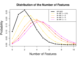
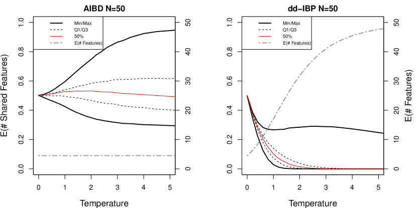
After fixing $\alpha=1$, $N=5$, and using the permutation of increasing natural numbers 1 through $N$, we obtain the probability distribution of the number of features as shown in Figure 1. Recall that both $T_{AIBD}$ and $T_{IBP}$ have the same distribution as $T$, whereas the number of non-zero columns in the dd-IBP, $T_{dd\text{-}IBP}$, varies by temperature and distance information. The distributions of $T$ and $T_{dd\text{-}IBP}$ were given in (11) and (12). Figure 1 illustrates that, for this proximity matrix, the dd-IBP has a higher number of expected features than the IBP. As the temperature increases, $T_{dd\text{-}IBP}$ has a limiting distribution of a Poisson($\alpha N$), and values on the off diagonal of the dd-IBP’s proximity matrix approach zero. Thus, the proximity matrix $\bm{P}$ approaches an identity matrix, and $\alpha\sum_{i}^{n}(1/h_{i})\rightarrow\alpha N$ as $\tau\rightarrow\infty$. In this case, the $N$ customers do not share features and individually sample $\alpha$ dishes, on average. On the other hand, the AIBD preserves the same distribution of the number of features as the IBP, regardless of temperature, and is only affected by the mass parameter. This is an important attribute of the AIBD, because as the number of features increases so does the computational complexity of inference. The AIBD also encourages more feature sharing than the dd-IBP, as discussed in the next section.

Another property the AIBD preserves from the IBP is that they have the same expected number of features per customer, which is $\alpha$ (see Section S.1 in the supplementary material for a proof). These two properties ensure that the average number of features and the average number of features per customer are identical between the AIBD and the IBP. Therefore, the IBP and the AIBD do the same amount of feature sharing, which is solely controlled by the parameter $\alpha$. However, the AIBD differs from the IBP, not by changing the amount of feature sharing, but by allowing the propensity of customers to share a feature to depend on their pairwise distances.

Figure 1: The distribution of $T_{AIBD}$ and $T_{IBP}$ is displayed as the bold black line. The distribution of $T_{dd\text{-}IBP}$ is displayed in the narrow colored lines for various temperatures. This figure shows that the distribution of the number of features for the dd-IBP (using the proximity matrix in Table 1 and when $\tau>0$) is stochastically greater than the number of features for the IBP and the AIBD.

4.2 Expected Number of Shared Features

One consequence of exchangeability in the IBP is that the expected number of shared features is identical for all customer pairs. This is not a desirable property when, a priori, one knows that a pair of customers are more alike when compared to another customer. The AIBD is able to include this information; which has the desired effect of changing the expected number of shared features for a pair of customers, while the average overall feature sharing remains the same as with the IBP.

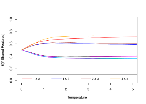
In the AIBD, customers that are closer in distance tend to share more features. The degree to which customers share features can be adjusted by the temperature parameter. An example is shown in the plot of Figure 2. The plot was obtained by fixing $\alpha=1$ and by using pairwise similarity information found in Table 1. We fixed $\alpha$ because changing the mass parameter only scales the y-axis in the plot of Figure 2. The lines indicate the expected number of shared features for a pair of customers.

AIBD Similarity Matrix ($\tau=1$) 1 2 3 4 5 1.00 0.89 0.51 0.02 0.02 0.89 1.00 0.55 0.03 0.02 0.51 0.55 1.00 0.04 0.03 0.02 0.03 0.04 1.00 0.36 0.02 0.02 0.03 0.36 1.00

Figure 2: The expected number of shared features as a function of temperature in the AIBD (averaged over all permutations) with corresponding similarity matrix when $\tau=1$. Each line represents a customer pair, with some pairs identified in the legend. This figure shows that the AIBD adjusts feature sharing for pairs of customers given the similarity matrix; the IBP would have all customers share on average 0.5 features.

When the temperature is zero, the AIBD reduces to the IBP, and so all customer pairs have the same expected number of shared features. Due to variability between permutations, each line in Figure 2 was calculated by averaging the expected number of shared features across all possible $N!=120$ permutations. In other words, $\bm{\rho}$ was integrated out after placing a uniform prior on it. Since $N$ is small, we enumerated across all permutations up to 7 possible features, which accounted for 99.4% of the probability mass.

A similarity matrix from a fixed temperature is shown to the right of the feature sharing plot in Figure 2. As expected, customers with higher similarity tend to share more features. However, even though customers 1 and 2 have the highest similarity, customers 4 and 5 tend to share more features. This behavior occurs by design, the expected number of features per customer in the AIBD is the same as in the original IBP, so the distances do not effect the number of features, just how features are shared among each other. So, the issue is not which $\exp\{-\tau d_{i,j}\}$ is the largest or smallest, but rather the relative sizes of these quantities. See (9) and (10). As an illustration, consider the similarity matrix in Figure 2 and suppose that customer 5 is the last to be allocated features. Among customers 1–4, customer 5 will highly favor sharing features with customer 4 since the relative similarity $0.36/(0.02+0.02+0.03+0.36)=0.84$ is close to 1. Conversely, if customer 1 is the last to be allocated, its relative attraction to customer 2 is only $0.89/(0.89+0.51+0.02+0.02)=0.61$, which is not as large as 0.84. Therefore, it would be expected that even though customers 1 and 2 have the highest similarity (i.e., 0.89), customers 4 and 5 tend to share more features. The sharing arrangements will depend somewhat on the permutation since, a priori, feature allocation only depends on the similarities of previously allocated customers, but the overall effect remains that number of shared features among pairs of customers will be driven by relative rather than absolute similarities. Table S.2 in the supplementary material compares the expected number of features between two states with the similarity values for this example with three different temperatures.

We now examine the effect of increasing $N$ on the expected number of shared features per customer in the AIBD. We do this using plots similar to Figure 2. Additionally, we use plots for both the AIBD and dd-IBP to compare how they each influence feature sharing. We use sample sizes $N=5$ and $N=50$ to demonstrate the effect of increasing $N$. Since it is computationally infeasible to enumerate $50!$ permutations, we create the plots using Monte Carlo estimation.

To sample from the AIBD with a greater number of customers, we used pairwise distance information from the $N=50$ states in the USArrests dataset in R. To obtain the similarity matrices used, first we centered and scaled the USArrests dataset. Then, we calculated a pairwise symmetric Euclidean distance matrix based on all the data. For $N=50$, we simply used all states, but for $N=5$ we used the same states that were used to calculate Table 1, which were centered and scaled separately. The simulation results for the AIBD are shown in the top row of Figure 3.

Figure 3: A view of the average feature sharing as a function of temperature for the AIBD and dd-IBP using sample sizes of $N=5$ and $N=50$, where $\alpha=1$. This figure shows how the AIBD retains the overall average of the expected number of shared features of the IBP, while on average the dd-IBP with a sequential proximity matrix shares less, as the temperature increases. For each plot the permutation of the data, $\bm{\rho}$, was integrated out of the model, similar to Figure 2 but using Monte Carlo integration.

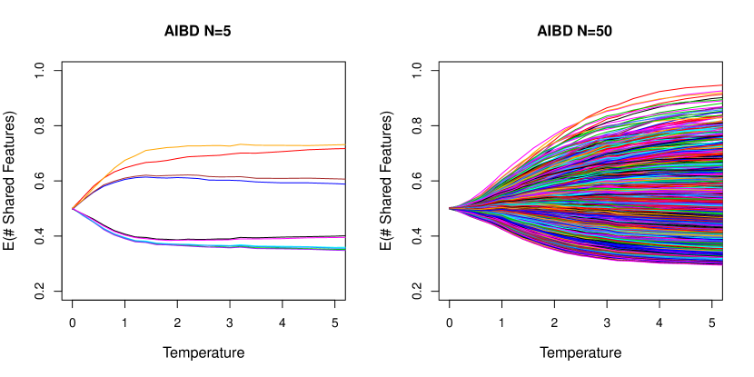
Note that in the IBP, which corresponds to the AIBD with $\tau=0$, the expected number of shared features between all customer pairs is $\alpha/2$. For any $N$, due to exchangeability, the number of shared features is the same for all customer pairs. Recall that the first customer samples $X_{1}\sim\text{Poisson}(\alpha)$ dishes. The second customer will take each dish sampled by customer 1 with probability $1/2$. Thus the total number of shared features between customers 1 and 2, is $X_{1,2}\sim\text{Binomial}(X_{1},1/2)$. By the law of total expectation, $E(X_{1,2})=E(E(X_{1,2}|X_{1}))=E(X_{1}/2)=\alpha/2$. Since any permutation of customers results in the same probability distribution for the IBP, the expected number of shared features for the first and second customer is the same for other pairs. While the AIBD is not exchangeable, it can be shown by simulation that across any temperature $\tau$ and sample size $N$, the expected number of shared features averaged across all pairs is $\alpha/2$. Thus, the AIBD allows each pair to share features differently; but across all pairs, the mean of the expected number of shared features is the same as the IBP.

For the AIBD, as customers are added to the process (i.e., as $N$ grows) the behavior of the average feature sharing changes, as seen in the top two plots of Figure 3. For high temperatures, a customer pair can share, on average, more or less than when there are more customers in the restaurant. At $\tau=5$ and $N=5$, the expected number of shared features for the 10 possible pairs range from $0.35$ to $0.73$, when $N=50$ this range increases by roughly 60% for those same pairs. Thus increasing $\tau$ and $N$ allows more disparity between the average feature sharing of customer pairs.

4.3 Comparison of the AIBD’s and the dd-IBP’s Properties

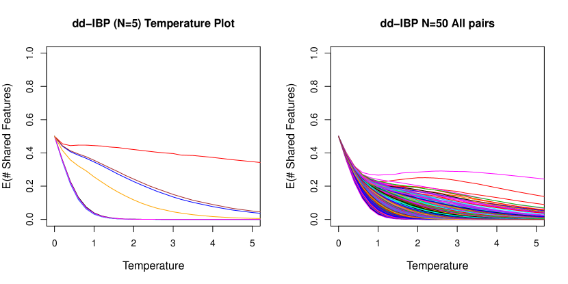
Although both use the pairwise distances of items, the AIBD and the dd-IBP have some notable differences. To compare the AIBD’s properties to the dd-IBP’s, we refer to Figure 3. The bottom row of the figure shows that as the temperature increases in the dd-IBP, on average, pairs of customers share less. Asymptotically, all average feature sharing goes to zero; that is, at a temperature of infinity, all customer pairs will share no features. We find similar behavior for the dd-IBP with a symmetric proximity matrix; plots for that distribution, similar to Figure 3, can be found in Figure S.1 in the supplementary material. Additional exploration of feature sharing in the AIBD and the dd-IBP can be found in Section S.3 of the supplementary material.

A table comparing several properties of the AIBD and dd-IBP to the IBP is shown in Table 2. In the dd-IBP, on average the customers share less as $\tau$ increases. As a result, all lines in the dd-IBP plots in Figure 3 go to zero as $\tau\rightarrow\infty$. This may be sensible in cases where we want customers to share less than the IBP. However, it does not seem possible to allow certain customer pairs to share more than the IBP. In contrast, the AIBD up-weights or down-weights average sharing depending on the pairwise similarity value while still having the same average expected number of shared features across all pairs as the IBP. Larger $N$ increases the disparity between pairs in the AIBD, but appears to decrease the disparity between pairs for the dd-IBP.

Property	AIBD	dd-IBP
Tractable pmf	Yes	No
Reduces to IBP when $\tau=0$	Yes	In one case
E(# Features)	Same as IBP	Different from IBP
E(# Features per customer)	Same as IBP	Different from IBP
E(# Total shared features)	Same as IBP∗	Different from IBP∗∗
E(# Shared features per customer)	Higher or Lower	Different from IBP∗∗

Table 2: Summary of the properties of the AIBD and dd-IBP to the IBP. Details of the first two properties can be found in Section 3, and the remainder can be found in Section 4, focusing on the dd-IBP’s properties in Section 4.3. $*$ Demonstrated via simulation. $**$ We consistently found this to be lower than the IBP in simulations.

For the dd-IBP, a major consequence of the expected number of shared features going to zero as $\tau\rightarrow\infty$ is that the total number of features in the distribution increases to $\alpha N$. For $N=50$ and $\alpha=1$, the expected number of features in the AIBD is the 50th harmonic number, or 4.5 for all temperatures. For the dd-IBP in this example, however, the expected number of features can range from 4.5 to 50, depending on the temperature chosen. This is shown in Figure 4. The dd-IBP reduces sharing and borrowing of strength between features, which is a primary reason to use the IBP. This can potentially result in higher computational burdens when a $\bm{Z}$ from the dd-IBP has a larger number of columns than the AIBD. One reason why the average number of shared features in the AIBD does not tend to zero is that the AIBD preserves the distribution of the total number of features for fixed $\alpha$ and $N$. Thus, in the AIBD, the distribution of the number of columns is unchanged from the IBP. The AIBD only influences how features are shared.

Figure 4: The distribution of the total number features overlayed with the pairwise expected shared feature plots for the AIBD and the dd-IBP for $N=50$. The Q1 and Q3 lines represent the quartiles of the number of shared features. This figure highlights that as the temperature increases, the average number of features (gray dashed line) remain fixed in the AIBD, but grows rapidly in the dd-IBP. It also shows how the median number of shared features (red line) of the AIBD and the dd-IBP change as a function of temperature.

The primary point of both the dd-IBP and the AIBD is that two data points with similar covariates should generally share more features than two with less-similar covariates. However, our approach to achieving this differs from the dd-IBP on a key point. In the AIBD, the total number of features (and, therefore, the total amount of sharing) is controlled with the mass parameter $\alpha$. It is not influenced by the similarity/proximity matrix. Further, we also designed the AIBD such that the similarity matrix has the sole influence on how the total amount of sharing (as determined by the mass parameter) is divided. For example, the IBP with a particular value for the mass parameter induces a distribution over the amount of sharing. The AIBD, with this same value for the mass parameter, also has the same total amount sharing on average, but the AIBD provides the flexibility to divide it according to the similarity matrix. In contrast, the dd-IBP uses the pairwise distance information to influence both the number of features and the sharing configurations. That is, although both are based on pairwise distances, the AIBD and dd-IBP use them to achieve fundamentally different distributions and, together, they provide choice for the statistician.

4.4 The Similarity Function

The similarity function can be chosen to accommodate a variety of feature-sharing behaviors. Figure 5 shows the transpose of the feature allocation $\bm{Z}$ simulated under the constant, reciprocal (with shift$=$1), window (with width$=$2), and exponential functions. A mass of $\alpha=5$, a temperature of $\tau=2$, and the absolute temporal distance ($d_{i,j}=|i-j|$) for 100 customers were used. The same random number generator seed was used to generate the figures, so the first two customers in each scenario take the same dishes. Note that the constant similarity reduces the AIBD to the IBP.

(a) Constant similarity function	(b) Reciprocal similarity function
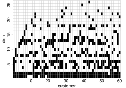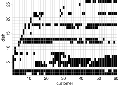(c) Exponential similarity function	(d) Window similarity function

Figure 5: A draw from the AIBD under the (a) constant, (b) reciprocal, (c) exponential, and (d) window functions. For the window similarity, a width of 2 was used; for the reciprocal similarity, a shift of 1 was used. For all simulations, the number of customers $N$ was 60, the mass $\alpha$ was 5, the permutation was $\{1,\dots,N\}$, the temperature $\tau$ was 2, and the distance used was the absolute temporal distance ($d_{i,j}=|i-j|$).

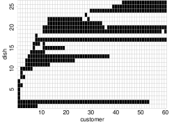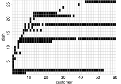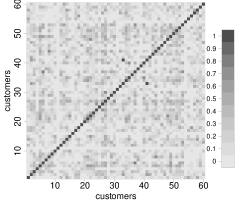
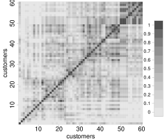
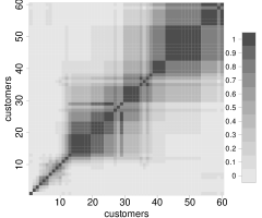
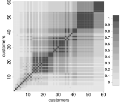
Considering the correlation structures between observations can provide additional intuition for selecting the similarity functions. To illustrate, Figure 6 provides a view of the squared correlation between customers, computed from the feature allocations under the four similarity functions. Unsurprisingly, under the IBP (constant similarity), correlations between proximal customers are weak. Under the exponential and window similarity for the temperature of 2, strong correlations are observed between proximal customers. Correlations appear to diminish as customers get further apart. Under the reciprocal similarity with a shift of 1 and temperature of 2, the correlation structure is less pronounced. Moderate correlation can be observed between proximal customers, but weakens at longer ranges.

(a) Constant similarity function	(b) Reciprocal similarity function
(c) Exponential similarity function	(d) Window similarity function

Figure 6: Squared correlation matrix between customers drawn from the AIBD under various similarity functions.

4.5 Lack of Marginal Invariance

Unlike the IBP, the AIBD and dd-IBP are not marginal invariant. Both distributions are such that the distribution defined for $n-1$ customers is not the same as the distribution obtained by marginalizing over the last customer. Thus, data analysis with the AIBD and dd-IBP is limited to cases where we are fully aware of the pairwise distances among all data points. By construction and as desired, adding another observation changes the relative relationships among the previous observations. Take, for example, the AIBD similarities in Table 1. If New Hampshire was never considered, Iowa and Wisconsin will share more features because they are relatively closer. Conversely, having New Hampshire in the model greatly changes the relative relationships, an effect that persists even when marginalizing over New Hampshire.

5 AIBD Posterior Sampling

We now describe how to sample from the joint posterior distribution of the model parameters in the LGLFM (i.e., $\bm{Z}$, $\tau$, $\alpha$, $\bm{\rho}$, $\sigma_{A}$ and $\sigma_{X}$), presented in Section 2.3, with an AIBD prior on the feature allocation. We suggest priors for the parameters and a Metropolis-Hastings-within-Gibbs sampling algorithm. Using the likelihood in (8), we can write the full joint posterior as shown in the following equation:

$$p(\bm{Z},\bm{\rho},\alpha,\tau,\sigma_{X},\sigma_{A}|\bm{X},\bm{\Lambda})\propto p(\bm{Z}|\alpha,\bm{\rho},\tau)~{}p(\bm{\rho})~{}p(\alpha)~{}p(\tau)~{}p(\sigma_{X},\sigma_{A})~{}p(\bm{X}|\bm{Z},\sigma_{X},\sigma_{A}).$$ (13)

5.1 Posterior Sampling of the Feature Allocation Z

We use an AIBD prior on $\bm{Z}$ along with prior distributions on the other parameters in conjunction with the likelihood, and suggest the following algorithm to sample from the posterior. We emphasize that this algorithm is valid only for the collapsed likelihood defined in (8). We suppose it could be adapted to other prior distributions on $\bm{Z}$.

From (13), the full conditional distribution of $\bm{Z}$ is proportional to

$$p(\bm{Z}|\alpha,\bm{\rho},\tau)~{}p(\bm{X}|\bm{Z},\sigma_{X},\sigma_{A}).$$

Instead of proposing an entirely new $\bm{Z}$ matrix, we update $\bm{Z}$ row-by-row. Define a singleton feature for row $i$ to be a feature that only customer $i$ has. In other words, a singleton feature for customer $i$ is a column in $\bm{Z}$ of all zeros except for a 1 on row $i$. Define the non-singleton features to be features that are owned by any of the other customers. For each row $i\in\{1,2,\ldots,N\}$ in $\bm{Z}$:

1. Let $m_{1},m_{2},\ldots m_{h}\in\mathcal{K}$ be the collection of column indices of the non-singleton features in the current state of $\bm{Z}$, where $h$ is the total number of non-singletons. If $h=0$, skip to step 3. If $h>0$, generate a random permutation of the collection of indices in $\mathcal{K}$. We update the non-singleton columns in this order in step 2.

2. Start by updating the non-singleton features on row $i$ one at a time using the Metropolis-Hastings algorithm in the permuted order as generated in step 1. Denote $z_{i,m}$ to be the binary number in the $i^{th}$ row and $m^{th}$ column of $\bm{Z}$. We update each element $z_{i,m}$ for each $m\in\mathcal{K}$ sequentially according to the permutation of $\mathcal{K}$. For each $m\in\mathcal{K}$:

   1. Define the active feature to be the feature in the $m^{th}$ column of the current state of $\bm{Z}$. This is the feature that is currently being updated.

   2. Propose $z^{*}_{i,m}=1-z_{i,m}$ (i.e., the opposite of the current state of $z_{i,m}$). Let $\bm{Z^{*}}$ be the same as $\bm{Z}$, except for $z^{*}_{i,m}$ in place of $z_{i,m}$.

   3. Since the order of the columns does not matter, different updates may result in the same proposed feature allocation. Thus, the proposal distribution is not symmetric. The Hastings ratio is computed by dividing the number of features identical to the active feature $d^{*}$ in $\bm{Z}^{*}$ by the number of features identical to the active feature $d$ in $\bm{Z}$. The active feature is also counted in this total, so if the active feature is distinct in both the current and proposed states, the ratio is 1. From the example in Figure 7, $m=4$ and $h=4$, and the active feature is column 4. In the current state, there are $d=2$ features identical to column 4 (including itself), and $d^{*}=3$ features identical to column 4 in the proposed state.

   4. Compute the Metropolis-Hastings ratio $MHR=\frac{p(\bm{Z^{*}}|\alpha,\bm{\rho},\tau)p(\bm{X}|\bm{Z}^{*},\sigma_{X},\sigma_{A})}{p(\bm{Z}|\alpha,\bm{\rho},\tau)p(\bm{X}|\bm{Z},\sigma_{X},\sigma_{A})}\frac{d^{*}}{d}$ and update $z_{i,m}$ to $z_{i,m}^{*}$ with probability min(1, $MHR$), else leave $z_{i,m}$ unchanged.

3. Now we propose new singleton features for customer $i$.

   1. We first evaluate the unnormalized probability mass of the full conditional distribution of $\bm{Z}$ after adding $0,1,2,\ldots$ features (with all other parameters and rows in $\bm{Z}$ held constant). Since we cannot check a theoretically infinite number of features, we stop considering new features once we obtain a mass that is less than a specific fraction (e.g., we used $1/1000$) of the highest mass. This should cover most reasonable posterior values and the fraction is a tuning parameter that can be adjusted if desired. This truncation step makes this algorithm an approximate sampler, but it can closely mimic an exact sampler. See Section S.2 in the supplementary material for a simulation study on the accuracy of this sampling algorithm.

   2. We estimate probabilities $p_{0},p_{1},p_{2},\ldots$ of adding 0,1,2,…singleton features by dividing each unnormalized mass in the previous step by the sum of all masses. Add $j$ singletons to customer $i$ with probability $p_{j}$.

Current State $\bm{Z}$

$\begin{bmatrix}1&0&1&\underline{0}&1\\ 1&1&0&1&1\\ 0&0&0&0&0\\ \end{bmatrix}$

Proposed State $\bm{Z}^{*}$

$\begin{bmatrix}1&0&1&\underline{1}&1\\ 1&1&0&1&1\\ 0&0&0&0&0\\ \end{bmatrix}$

Figure 7: Example of a posterior update from step 2. Customer 1 has one singleton feature (column 3) and four non-singleton features. For customer 1, we will individually update the columns 1,2,4, and 5 in a random order. The underlined number $z_{14}$ is being updated and thus the active feature is column 4. There are 3 features identical to the active feature (including itself) in the proposed state and 2 identical features in the current state. The Hastings ratio is 3/2 to account for the asymmetric proposal.

After going through all rows, the result is one scan of the Markov chain updates for $\bm{Z}$. We then sample from the other parameters, which we describe in the next section.

5.2 Sampling the Other Parameters

After updating $\bm{Z}$, we proceed to update the other parameters ($\alpha$, $\bm{\rho}$, $\tau$, $\sigma_{X}$, and $\sigma_{A}$). The parameters $\alpha$ and $\tau$ are sampled univariately; while $(\sigma_{X},\sigma_{A})$ is sampled jointly, and $\bm{\rho}$ is sampled as a vector.

For the mass parameter $\alpha$, we suggest using a gamma prior because it is conditionally conjugate. If a Gamma($a_{\alpha}$, $b_{\alpha}$) prior (with expectation $a_{\alpha}/b_{\alpha}$) is used, then the resulting conditional posterior is a draw from a Gamma($a_{\alpha}+T_{\bm{Z}}$, $b_{\alpha}+H_{N}$). $T_{\bm{Z}}$ indicates the total number of features in the current state of $\bm{Z}$ and $H_{N}$ is the $N^{th}$ harmonic number.

For the permutation parameter $\bm{\rho}$, we suggest using a discrete uniform on all possible permutations of the integers 1 through N, unless there is natural ordering in the data. Using the discrete uniform prior, we update $\bm{\rho}$ with a random walk using a discrete uniform proposal. For small N, this can be done by sampling from any of the $N!$ possible permutations. However, for larger $N$, this could lead to low acceptance rates. As such, we recommend only updating $k_{\rho}$ of the elements in the permutation at a time, where $k_{\rho}$ is a tuning parameter that controls how quickly the permutation space is explored. In our experience choosing $k_{\rho}$ to obtain an acceptance rate of around 25% produced good mixing. As $N$ gets larger, $k_{\rho}$ may need to stay at a fixed quantity to get good acceptance rates. The steps to sample a new $\bm{\rho}$ are outlined as follows. First randomly select $k_{\rho}$ indices in the permutation to update. Next, randomly shuffle the $k_{\rho}$ indices, while leaving the other $N-k_{\rho}$ indices fixed, to generate a proposed permutation. Finally, calculate the Metropolis acceptance ratio, $R_{\rho}$ and accept the proposed permutation with probability min(1, $R_{\rho}$). Checking for good mixing and convergence for $\bm{\rho}$ is more nuanced than for the other parameters. We provide some recommendations in Section 6.5 to assess the convergence for $\bm{\rho}$.

The temperature parameter $\tau$ in the likelihood does not appear to have a conjugate prior. Therefore, any prior with positive continuous support might be reasonable. For our implementation, we choose a Gamma prior. To draw from the conditional posterior of $\tau$ we use a Metropolis step with a Gaussian random walk proposal and reject proposals outside the support of $\tau$.

For the variance components of the likelihood, we recommend using any positive continuous prior, such as a Gamma prior on $\sigma_{X}$ and $\sigma_{A}$. Since $\sigma_{X}$ and $\sigma_{A}$ are typically negatively correlated in the posterior, we used a bivariate Gaussian random walk to update both parameters simultaneously, again rejecting proposals outside the support of $(\sigma_{A},\sigma_{X})$.

Due to the computational burden of updating $\bm{Z}$ relative to updating the other parameters, we recommend updating the other parameters several times for every update of $\bm{Z}$. We updated other parameters 10 times for every update of $\bm{Z}$ in the application in Section 6 to reduce the autocorrelation within the posterior draws, at a negligible computational cost.

The methods suggested in this section are implemented in the samplePosteriorLGLFM function of the aibd R package. The posterior sampling algorithm can be applied to both the AIBD and, since it is a special case of the AIBD, the IBP. From our experience, the results are accurate and the only source of bias comes from the truncation step. This truncation error can be controlled and appears to be negligible compared to Monte Carlo error.

6 Data Analysis

In this section, brain measurement data is analyzed using a latent feature model in several analyses. The LGLFM likelihood, introduced in Griffiths and Ghahramani (2006) and discussed in Section 2.3 of this paper, remains the same over each analysis, however, the prior distributions vary. Three fundamentally different prior distributions are considered. Specifically, the proposed AIBD, the dd-IBP and the standard IBP are used as prior distributions on the matrix $\bm{Z}$ and the posterior results are then compared.

6.1 The Data

The data for these analyses were obtained from a neuroimaging study of the brains of healthy and Alzheimer’s-diseased subjects (see Dinov et al., 2009). The data and some details of the study are available on UCLA’s Statistics Online Computational Resource (SOCR) data page SOCR (2009). Of that data, we consider the 27 Alzheimer’s diseased and 35 normal control subjects. In the study, 56 distinct regions of interest (ROIs) in the brain are observed; each region has four different measurements. The four measurements are the surface area (SA), shape index (SI), curvedness (CV), and fractal dimension (FD). One of the properties of the LGLFM is that the error terms for each of these measurements are assumed to have constant variance. Therefore, before modeling, the ROI measurements are centered and scaled (so each has a mean of zero and a standard deviation of one). Additionally, the SA measurements are somewhat skewed, thus a log transformation was performed before centering and scaling those measurements.

6.2 The Analysis

The analysis of this data mirrors the steps taken in Gershman et al. (2015). First, patient age is included in the AIBD and dd-IBP priors as a distance between patients. Including this distance makes the both the AIBD and dd-IBP priors nonexchangeable, with the hope that this extra information will improve the model’s predictive performance. The distances between patients are defined in both priors using the exponential decay function (i.e., $\exp\{-\text{temperature}\times|\text{age difference}|\}$). As in their analysis, we use a sequential proximity matrix for the dd-IBP and fix the order of the patients from youngest to oldest in both the AIBD and the dd-IBP. The temperatures for the AIBD and dd-IBP are set at 5 levels (0.4, 0.8, 1.2, 1.6, and 2.0). Since the IBP prior is exchangeable, it does not include any distance information between patients. In each model a gamma$(1,1)$ is used as the prior distribution for the mass parameter (the same as in the dd-IBP code by Gershman, 2013). The LGLFM likelihood is used as defined previously, with the data being the 4 different measurements in 56 regions of the brain. The data, $\bm{X}$, are contained in a 62 $\times$ 224 matrix, which is an over parameterized model unless some type of regularization or dimension reduction is used.

Prior distributions for the variance components of the likelihood also need to be specified. Since the data are centered and scaled, a reasonable maximum value for $\sigma_{A}$ and $\sigma_{X}$ is 1. Therefore, in all models a standard uniform prior is placed on these parameters; i.e., $p(\sigma_{A})=\text{I}\,(0<\sigma_{A}<1)$ and $p(\sigma_{X})=\text{I}\,(0<\sigma_{X}<1)$.

With the models fully specified, we follow similar steps of the analysis in Gershman et al. (2015). First, we obtain 3,000 MCMC posterior samples from each model. The first half of the samples is discarded for burn-in. Each model had 50 MCMC chains, for a total of 75,000 posterior samples. For each sample, the subjects are randomly divided into training and testing sets. Using the latent features from the posterior sample of $\bm{Z}$ as predictors, an L₂-regularized logistic regression is performed on the training set (to classify which patients do or do not have Alzheimer’s disease). For the logistic regression, we use the penalized function in the penalized R package (Goeman et al., 2018; Goeman, 2010) with the regularization constant set to $10^{-6}$. Using the results from the logistic regression model, the test group subjects are then classified to assess performance. Finally, for each test group’s classification, the area under the receiver operating characteristic curve (AUC) is calculated. Thus we obtain 75,000 posterior samples of AUC, which are used to compare each model’s efficacy.

Although the steps in this analysis are the same as in Gershman et al. (2015), based on the information provided in that article, a few aspects of the analysis cannot be replicated. First, in the dd-IBP paper a few observations were randomly removed in the classification to balance the training and testing sets. However, the removed observations were not identified. Therefore, we do not ignore any observations; i.e., the training and testing sets are disjoint but include all 62 subjects. Also, it is not specified which observations are assigned to the training and testing sets for classification. In our implementation, we randomly assign 14 diseased and 18 healthy subjects to the training set, and then assign the remaining 13 diseased and 17 healthy subjects to the testing set; this is repeated for each posterior sample.

In total there are five AIBD priors (one for each temperature), five dd-IBP priors, and one IBP prior. In each of those 11 models we obtained 75,000 posterior samples; the $i^{\text{th}}$ sample of each chain are compared using identical training and testing sets during classification. For posterior simulation, the code available at Gershman (2013) is used for the dd-IBP, and the functions included in the aibd package (Dahl et al., 2021) are used for both the AIBD and the IBP. Posterior means and standard deviations of the parameters from the several models are included in Section S.4 of the supplementary material. One possible confounding factor in our comparison of the AIBD and the dd-IBP is that the posterior simulation for the dd-IBP is an approximate MCMC scheme, as noted in Gershman (2013).

6.3 Comparison Between the AIBD and the dd-IBP

Each model’s performance is measured by how well it correctly classifies subjects into “healthy” or “diseased”. This performance can be quantified using the AUC, which ranges between zero and one, with higher values indicating a better classifier. Using the AUC, from the classifications on the testing sets, the results of the models with AIBD and dd-IBP priors are compared. 95% Monte Carlo confidence intervals for the expected posterior AUC from the models with AIBD and dd-IBP priors are reported in Table 3. This table shows that, on average, the AIBD has higher AUC than the dd-IBP at every temperature setting. In Table 4 we also include the deviance information criterion (DIC) scores (as defined by Gelman et al. (2013) and use the penalty term in their Equation 7.8), for each model to determine which has a better fit. The DIC indicates that the AIBD is performing better than the dd-IBP.

Temp	0.4	0.8	1.2	1.6	2.0
AIBD	(0.747, 0.748)	(0.747, 0.748)	(0.750, 0.752)	(0.754, 0.755)	(0.753, 0.754)
dd-IBP	(0.677, 0.679)	(0.715, 0.716)	(0.708, 0.710)	(0.719, 0.721)	(0.720, 0.721)

Table 3: Posterior Expected AUC. 95% Monte Carlo confidence intervals for the expected posterior AUC for the five AIBD and dd-IBP models (with fixed temperatures and permutation), higher values indicate better model performance.

Temp	0.4	0.8	1.2	1.6	2.0
AIBD	32531.58	32523.37	32557.66	32513.63	32489.31
dd-IBP	35322.27	35005.67	35286.97	35316.80	35144.78

Table 4: DIC values for the five AIBD and dd-IBP models (with fixed temperatures and permutation), lower values indicate better model fit.

While the AIBD performs better than the dd-IBP under these conditions, it has the added benefit of easily accommodating a prior on the temperature parameter. Finding a suitable static value for the temperature parameters seems neither intuitive nor straight-forward. Allowing prior distributions to incorporate some amount of uncertainty is arguably more appropriate. An additional model with an AIBD prior was fit (with 75,000 posterior samples) with a gamma$(1,1)$ prior distribution set on the temperature parameter and a uniform distribution on the permutation, $\bm{\rho}$. When taking advantage of this flexibility the AIBD performs even better, with a 95% Monte Carlo confidence interval on the expected posterior AUC of $(0.758,0.760)$, and a DIC of 32477. It should be noted that it is also possible to set a prior on the permutation for the dd-IBP, but the available software does not have that option. This example demonstrates that the AIBD prior is better able to capture the distance information (age) between subjects. On average, the logistic regression trained on each posterior $\bm{Z}$, learned from the AIBD model when compared to the dd-IBP model, more accurately classifies subjects as “healthy” or “diseased.”

To further compare the AIBD and the dd-IBP, the expected number of posterior features in $\bm{Z}$ can be found in Table 5. These numbers demonstrate a substantial reduction in dimension from the original 224 data columns plus the age variable. This reduction in dimension is really larger than it first appears because the entries in feature allocation matrices are binary, zeros and ones, whereas the data contained in $\bm{X}$ are continuous values. To determine how much information from the data is lost in the dimension reduction, we compare the AUC results from two alternative models. These alternative models are penalized logistic regressions fit to the same training sets of the centered and scaled data as the AIBD and dd-IBP models, one includes $\bm{X}$ as the predictors, and the other includes both $\bm{X}$ and the age of each patient. The average AUC of these models are 0.778 and 0.785 respectively. So little information is lost in the dimension reduction and the AIBD’s posterior feature allocation can comprise nearly all the information about a patient’s disease state, while drastically decreasing the dimensionality. This reduction of dimension is most useful if the results can be interpreted.

Temp	0.4	0.8	1.2	1.6	2.0
AIBD	68 (61,76)	68 (61,76)	66 (60,73)	66 (59,73)	65 (59,72)
dd-IBP	87 (56,128)	104 (74,134)	95 (68,135)	105 (76,200)	105 (73,199)

Table 5: The average number of features in the posterior samples of $\bm{Z}$ for the AIBD and the dd-IBP at five different temperatures. Additionally, for each case, a 95% posterior probability interval for the number of features is shown in parentheses.

Temp	0.4	0.8	1.2	1.6	2.0
AIBD	4.3 (3.9,4.9)	4.5 (4.1,5.2)	4.7 (4.1,5.2)	4.8 (4.2,5.3)	4.9 (4.3,5.6)
dd-IBP	4.2 (3.6,4.8)	3.6 (3.1,4.1)	3.2 (2.9,3.7)	2.9 (2.5,3.3)	2.7 (2.3,3.1)

Table 6: The average number of customers per feature in the posterior samples of $\bm{Z}$ for the AIBD and the dd-IBP at five different temperatures. Additionally, for each case, a 95% posterior probability interval for the number of customers per feature is shown in parentheses.

As discovered in the prior exploration of the AIBD and the dd-IBP, we also see similar feature sharing trends in the posterior. Table 6 shows the average number of customers per feature in the posterior samples for each of the 10 models. These numbers indicate that the amount of feature sharing goes down in the posterior of the dd-IBP as the temperature parameter increases. While we see an increase in the amount of sharing in the AIBD for the same temperatures.

A very rough speed comparison of the posterior sampling algorithms for the dd-IBP and the AIBD showed that the dd-IBP could do one update of all parameters in roughly 13 seconds (using $\sim$25 cores), while the AIBD took approximately 70 seconds (using one core). There are a few issues that make a full comparison quite challenging. One is that the methods are implemented in different software; the dd-IBP takes advantage of MATLAB’s multi-threading capabilities, while the AIBD implementation is single-threaded. Additionally, each MCMC scan is highly dependent on the number of active features in the current iteration, and the dd-IBP had a higher average number of posterior features in $\bm{Z}$. The AIBD also gains a time advantage using compiled code.

6.4 Comparison Between the AIBD and the IBP

As demonstrated, the AIBD competes favorably with the dd-IBP as an effective nonexchangeable prior for latent feature models. In this application we also want to show that using a nonexchangeable prior can produce better results than when using an exchangeable prior, specifically the IBP. In this case the AIBD has the added advantage over the IBP of knowing a patient’s age and using it as a distance between patients. If a patient’s age is important to predicting Alzheimer’s disease the AIBD should outperform the IBP; however, if the information is not informative no benefit should be expected.

The comparison between the models with the AIBD and IBP priors uses the same scheme as in the previous subsections. The prior for the mass parameter in both models is a gamma$(1,1)$ distribution. Additionally for the AIBD model, a gamma$(1,1)$ prior is set on the temperature parameter and a uniform prior on the permutation. Again, we recommend the permutation parameter be integrated out of the model, unless there is meaningful order of the data. To tune the proposal distribution of the permutation parameter, we set $k_{\rho}=8$ which produced an acceptance rate of approximately 20% in that Metropolis-Hastings step.

For posterior results we get, DIC values for the AIBD and the IBP models are 32477.35 and 32539.26, respectively. Additionally, the average number of customers per feature in the posterior samples is 74 for the AIBD and 70 for the IBP. The average number of customers per feature is 4.6 for the AIBD and 4.1 for the IBP. The resulting posterior expected AUC for each model is 0.759 and 0.747 for the AIBD and IBP, respectively. A 95% confidence interval on the paired difference between average AUC for the AIBD and the IBP is $(0.011,0.013)$. The results are fairly convincing: the AIBD can use the extra distance information to obtain better classification results.

This example demonstrates that a patient’s age does contain information that is valuable in classifying patients into healthy and Alzheimer’s diseased states. It also shows that the AIBD prior is able to capture this distance information contained in a patient’s age to improve model performance.

An informal speed comparison of the posterior sampling algorithms for the IBP and the AIBD showed that the IBP could do one update of all parameters in roughly 63 seconds, while the AIBD took approximately 70 seconds. This comparison is easier to make than with the dd-IBP, since the algorithm and software implementation are the same. This application demonstrates that the computational penalty for using the nonexchangeable AIBD prior isn’t high, and improves model performance over the IBP prior.

6.5 Items for Consideration

Procedures to check the convergence of the MCMC chains are rather standard for most parameters of the model, however, since $\bm{\rho}$ is fairly novel, we highlight a few considerations for it. As with essentially any parameter, we cannot visit all possible values for $\bm{\rho}$ in posterior sampling, and we treat it much the same as any other parameter. Although we set a uniform prior on $\bm{\rho}$, we do not expect its posterior to be uniform. What we want to accomplish is obtain a sample which provides reasonable Monte Carlo estimates. We look for good acceptance rates and exploration around the space by first checking that the chaining is moving and, secondly, converging. To check for movement, we observe the standard deviation of each item’s permutation in each chain and ensure it is well above 0. To check for convergence, we monitor the mean of the permutation of the first half of the observations and we also monitor the mean of the permutation of the odd observations. If these two summaries of $\bm{\rho}$ show convergence, this provides evidence that the chain is sampling from the stationary distribution. Additional summaries of $\bm{\rho}$ may be warranted if concern about the mixing of $\bm{\rho}$ exists.

The scalability of sampling from feature allocation models seems to be somewhat limited from small to moderate $N$. Conducting a simple test, we ran the AIBD model with a random temperature and permutation using three different data sets with $N\in\{31,62,124\}$. The test first used $\bm{X}_{31\times 224}$, next $\bm{X}_{62\times 224}$, and finally $\bm{X}_{124\times 224}$. The average time it took for one Gibbs scan took on average 3.7, 20.4, and 195.5 seconds, respectively. All else being equal, as $N$ grows so will the number of features $K$. The average $K$ for those 3 tests are: 25.7, 36.7, and 78.8. We also ran the same tests for the IBP and the average time it took for one Gibbs scan took on average 3.7, 20.9, and 188.7 seconds and the average $K$ for those 3 tests are: 25.7, 36.7, and 78.6, respectively. Therefore we see that the AIBD and the IBP scale similarly. We suppose this occurs because the likelihood computations dominate those of the prior. We expect the dd-IBP would scale similarly for the same values of $N$. For larger $N$, the computation required to get samples from the posterior might be too computationally expensive. Thus other approaches might be required, e.g., variational inference. A few works on variational inference in feature allocation models include Teh et al. (2007), Doshi et al. (2009), and Ranganath et al. (2014).

The similarity function, which transforms distances into similarities, is an important modeling choice in the AIBD. We considered a slightly altered AIBD model, again with random temperature and permutation, but only changing the similarity function. The similarity function we chose for the comparison was the reciprocal function $1/(d_{i,j}+10^{-5})$. The results were fairly similar to those obtained using the exponential decay similarity function. This model has a DIC of 32539.38, a 95% Monte Carlo (MC) confidence interval for AUC is (0.751, 0.752) and for posterior expected number of features is (71.7, 71.8), and the average number of customers per feature in the posterior samples is 4.5. In this case, the model does not seem to be overly sensitive to the choice of the similarity function.

7 Conclusion

In this paper, a generalization of the IBP was developed to allow for customer dependence in the prior. It was demonstrated that after including pairwise distance information, the AIBD preserves many familiar properties of the IBP. We compared these properties of the AIBD to those of the IBP and dd-IBP, and summarized them in Table 2. Further, while the AIBD and dd-IBP attempt to generalize the IBP by including pairwise distance information, we have shown that the AIBD possesses several properties that make it particularly appealing. An instance of this was shown in the application in Section 6, where the AIBD outperformed the dd-IBP in terms of AUC. We note that the AIBD is constrained to cases where distances are symmetric, whereas the dd-IBP allows for non-symmetric distances.

Overall, the AIBD is an attractive solution for incorporating distance information into a prior distribution of a feature allocation. It retains many desirable properties of the IBP. For a fixed mass and temperature, it encourages more feature sharing between customers than the dd-IBP. Priors can readily be set on model parameters, such as the temperature. Last, but not least, this distribution and some associated methods are implemented in the aibd package in R (Dahl et al., 2021).

The authors thank the editor, associate editor, and two anonymous referees for their insightful comments that substantially improved this work. This work was supported, in part, by NIH NIGMS R01 GM104972.

Supplementary Material

S.1 The AIBD’s Expected Number of Features per Observation. A Proof that the AIBD has the Same Number of Expected Features as the IBP

Here, we show that the sum of each row in the feature allocation matrix from the AIBD (conditioned on the permutation $\bm{\rho}$, temperature $\tau$, and mass $\alpha$) has an expected value of $\alpha$. Recall that $X_{i}$ is the number of new dishes customer $i$ takes, and $Y_{i}$ is the number of dishes sampled before customer $i$ samples dishes. Let $Q_{i}$ be the number of previously-samples dishes that $i$ takes. Let $S_{i}=X_{i}+Q_{i}$ be the total number of dishes sampled by customer $i$. That is, $S_{i}$ is the sum of row $i$ in the feature allocation matrix $Z$. We will show that $E[S_{i}\mid\alpha,\bm{\rho},\tau]=\alpha$, and thus, $E[S_{i}\mid\alpha]=\alpha$, for all $i$. We will show this by strong mathematical induction.

First, note that $S_{1}=X_{1}$, and $X_{1}\mid\alpha,\bm{\rho},\tau\sim\text{Poisson}(\alpha)$. Thus, $E[S_{1}\mid\alpha,\bm{\rho},\tau]=E[X_{1}\mid\alpha,\bm{\rho},\tau]=\alpha$. Next, $S_{2}=X_{2}+Q_{2}$. Thus, $E[S_{2}\mid\alpha,\bm{\rho},\tau]=E[X_{2}+Q_{2}\mid\alpha,\bm{\rho},\tau]=E[X_{2}+X_{1,2}\mid\alpha,\bm{\rho},\tau]=E[X_{2}\mid\alpha,\bm{\rho},\tau]+E[X_{1,2}\mid\alpha,\bm{\rho},\tau]=\alpha/2+\alpha/2=\alpha$, where $X_{1,2}$ is the number of shared features between customers 1 and 2. (See 4.2 for why $E[X_{1,2}\mid\alpha,\bm{\rho},\tau]=\alpha/2$.)

Now, suppose that for some $i\in\mathbb{N}$, $E[S_{j}\mid\alpha,\bm{\rho},\tau]=\alpha$ for all $j\leq i$. Let $C_{i}=\sum_{j=1}^{i}f(\tau,d_{\rho_{j},\rho_{i+1}})$, then

$$E[S_{i+1}\mid\alpha,\bm{\rho},\tau] = E\left[X_{i+1}+\sum_{k=1}^{Y_{i+1}}z_{i+1,k}~{}\bigg{|}~{}\alpha,\bm{\rho},\tau\right]$$

$$= \frac{\alpha}{i+1}+E\left[\sum_{k=1}^{Y_{i+1}}z_{i+1,k}~{}\bigg{|}~{}\alpha,\bm{\rho},\tau\right]$$

$$= \frac{\alpha}{i+1}+E\left[\sum_{k=1}^{Y_{i+1}}\frac{h_{i+1,k}(\tau)\cdot i}{i+1}~{}\bigg{|}~{}\alpha,\bm{\rho},\tau\right]$$

$$= \frac{\alpha}{i+1}+\frac{i}{i+1}\cdot E\left[\sum_{k=1}^{Y_{i+1}}h_{i+1,k}(\tau)~{}\bigg{|}~{}\alpha,\bm{\rho},\tau\right]$$

$$= \frac{\alpha}{i+1}+\frac{i}{i+1}\cdot E\left[\sum_{k=1}^{Y_{i+1}}\frac{\sum_{j=1}^{i}f(\tau,d_{\rho_{j},\rho_{i+1}})\cdot z_{j,k}}{\sum_{j=1}^{i}f(\tau,d_{\rho_{j},\rho_{i+1}})}~{}\bigg{|}~{}\alpha,\bm{\rho},\tau\right]$$

$$= \frac{\alpha}{i+1}+\frac{i}{i+1}\cdot E\left[\sum_{k=1}^{Y_{i+1}}\sum_{j=1}^{i}\frac{f(\tau,d_{\rho_{j},\rho_{i+1}})}{C_{i}}\cdot z_{j,k}~{}\bigg{|}~{}\alpha,\bm{\rho},\tau\right]$$

$$= \frac{\alpha}{i+1}+\frac{i}{i+1}\cdot E\left[\sum_{j=1}^{i}\frac{f(\tau,d_{\rho_{j},\rho_{i+1}})}{C_{i}}\cdot\sum_{k=1}^{Y_{i+1}}z_{j,k}~{}\bigg{|}~{}\alpha,\bm{\rho},\tau\right]$$

$$= \frac{\alpha}{i+1}+\frac{i}{i+1}\cdot\sum_{j=1}^{i}\left(\frac{f(\tau,d_{\rho_{j},\rho_{i+1}})}{C_{i}}\cdot E\left[\cdot\sum_{k=1}^{Y_{i+1}}z_{j,k}~{}\bigg{|}~{}\alpha,\bm{\rho},\tau\right]\right)$$

$$= \frac{\alpha}{i+1}+\frac{i}{i+1}\cdot\sum_{j=1}^{i}\left(\frac{f(\tau,d_{\rho_{j},\rho_{i+1}})}{C_{i}}\cdot E[S_{j}\mid\alpha,\bm{\rho},\tau]\right)$$

$$= \frac{\alpha}{i+1}+\frac{i}{i+1}\cdot\sum_{j=1}^{i}\left(\frac{f(\tau,d_{\rho_{j},\rho_{i+1}})}{C_{i}}\cdot\alpha\right)$$

$$= \frac{\alpha}{i+1}+\frac{i}{i+1}\cdot 1\cdot\alpha$$

$$= \alpha.$$

Thus, $E[S_{i+1}\mid\alpha,\bm{\rho},\tau]=\alpha$ also. Therefore, by mathematical induction, $E[S_{i}\mid\alpha,\bm{\rho},\tau]=\alpha$, for all $i\in\mathbb{N}$. Since for all $(\bm{\rho},\tau)$, $E[S_{i}\mid\alpha,\bm{\rho},\tau]=\alpha$, we also obtain $E[S_{i}\mid\alpha]=\alpha$.

S.2 Simulation of MCMC Algorithm Accuracy. A Posterior Simulation Study to Show the Accuracy of the Proposed MCMC Algorithm

We conducted a Monte Carlo study to demonstrate that the proposed MCMC algorithm in Section 5.1 approximately samples from the target distribution. Recall that our algorithm has a truncation parameter, designed to provide feasible computation with reasonable accuracy. We consider our sampling algorithm for various truncation parameters and use our MCMC algorithm to sample $\bm{Z}$’s from the AIBD prior distribution. We also sample $\bm{Z}$’s using the constructive definition of the AIBD from Section 3. We then compare Monte Carlo estimates of univariate summaries of the distribution and compare them to theoretical values. The default value for the truncation parameter is $1000$ and we show that Monte Carlo error dominates the small truncation error.

The experiment has two measures of accuracy. The first finds the largest absolute difference of the empirical probability of getting a $\bm{Z}$ with $K$ features (for all possible $K$) and its actual probability. Recall $\bm{Z}$ is an $N\times K$ matrix, thus for $m$ samples we compute

$$\max_{\text{all }k}\ \Bigg{|}\,P(K=k)-\frac{1}{m}\sum_{i=1}^{m}I(K_{i}=k)\,\Bigg{|}.$$ (S.1)

The second measure of accuracy compares the average number of active features with the theoretical results. This is expressed as

$$\Bigg{|}\,\alpha N-\frac{1}{m}\sum_{i=1}^{m}tr(\bm{Z}_{i}{\bm{Z}_{i}}^{T})\,\Bigg{|}.$$ (S.2)

It would be more accurate to compare the number of times each $\bm{Z}$ was sampled with its theoretical probability, however, the space of all possible $\bm{Z}$ is too large, even for moderate $N$, to take this approach.

Sampling Method	Max. Prob. of Feature Error	Mean Active Feature Error
Monte Carlo	0.00024	0.0030
MCMC (trunc. $=$ 1000)	0.00024	0.0035
MCMC (trunc. $=$ 100)	0.00052	0.0102
MCMC (trunc. $=$ 10)	0.00210	0.1106
MCMC (trunc. $=$ 1)	0.00203	0.1255

Table S.1: This table provides two metrics on the accuracy of the proposed MCMC sampler from Section 5.1. It shows that the MCMC sampler with the truncation parameter set to 1000 is nearly as accurate as a Monte Carlo sample from the AIBD. As the truncation parameter decreases, so does the accuracy.

	$\tau$	1 / 2	1 / 3	1 / 4	1 / 5	2 / 3	2 / 4	2 / 5	3 / 4	3 / 5	4 / 5
Distance	–	0.12	0.66	3.74	3.78	0.59	3.65	3.69	3.32	3.46	1.01
Expected	$0.2$	0.54	0.53	0.48	0.47	0.53	0.48	0.48	0.48	0.48	0.53
Similarity		0.98	0.88	0.47	0.47	0.89	0.48	0.48	0.51	0.50	0.82
Expected	$1.0$	0.65	0.61	0.39	0.39	0.61	0.39	0.39	0.41	0.40	0.67
Similarity		0.89	0.51	0.02	0.02	0.55	0.03	0.02	0.04	0.03	0.36
Expected	$5.0$	0.72	0.59	0.35	0.35	0.61	0.36	0.36	0.40	0.39	0.73
Similarity		0.55	0.04	0.00	0.00	0.05	0.00	0.00	0.00	0.00	0.01

Table S.2: This table shows the expected number of features between two states compared with the similarity of those two states, for three different temperatures. As the temperature increases, the similarity (for this similarity function) decreases and the sharing of features also changes, it goes up for closer items and goes down for items that are relatively far apart.

Figure S.1: The expected number of shared features between two states as a function of temperature for the dd-IBP with a symmetric proximity matrix. In this case, the permutation is irrelevant because there is no ordering of the customers. As shown, the expected number of shared features has an initial increase and then decreases as the temperature parameter increases. Across all pairs of states and for all temperatures the amount of sharing is lower than the IBP.

Figure S.2: These four plots show the pairwise distances against the expected number of shared features in the AIBD when N$=$50 for different temperatures. The permutation parameter is integrated out (using Monte Carlo).

Figure S.3: These four plots show the pairwise distances against the expected number of shared features in the AIBD when N$=$50 for different temperatures. The permutation parameter is fixed using the alphabetical ordering of the states.

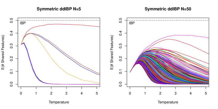
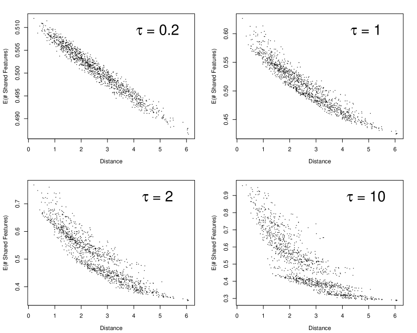
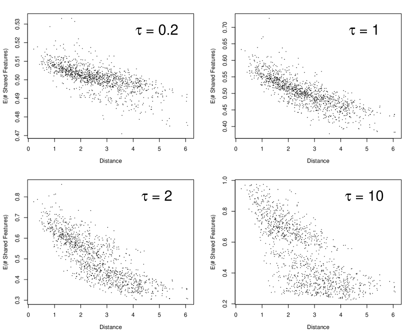
In this simulation we set $N=10$ and $\alpha=1.4$. The distance matrix is defined by $d(i,j)=|i-j|/N$, and we use the exponential decay function to transform the distances to similarities with $\tau=2$. The permutation is fixed at $1,2,\ldots,10$, and for thinning we retain every tenth sample. We obtain a total of one million samples for each case. We sample directly from the AIBD for one case and use the MCMC sampler to obtain posterior samples (with the likelihood proportional to 1) in the four other cases. Each of the four cases of the MCMC sampler use different truncation parameter settings $(1000,100,10,1)$.

The results are shown in Table S.1 where lower numbers represent lower error. The “Max Prob of Feature Error” column contain values from (S.1) and the “Avg Active Feature Error” column contain values from (S.2). It appears the second metric is more sensitive to deviations from the truth. In Table S.1 we also included a Monte Carlo estimate (sampling directly from the AIBD) to help quantify the amount of MC error one might expect. Clearly, the Monte Carlo sample, directly from the target distribution, is most accurate to the theoretical results. Our MCMC algorithm with the truncation parameter set to 1000 is also very close to the truth. When the truncation parameter is 100 the algorithm loses more accuracy and degrades as it decreases.

This experiment supports our claim that the proposed algorithm is samplingfrom the posterior directly, but it has some inherent truncation error. This error can be reduced by increasing the newFeaturesTruncationDivisor argument in theaibd::samplePosteriorLGLFM function. The default is set at 1000, where we have observed that this truncation error is much smaller than typical Monte Carlo error. A rough estimate from this simulation indicates that the computational expense from increasing the truncation parameter from 100 to 1000 is about 15%.

S.3 Additional Material on Feature Sharing

This section further explores the sharing of features beyond that of the manuscript. The data is from the USArrests dataset contained in R. When $N=5$, the states selected are New Hampshire, Iowa, Wisconsin, California, and Nevada (in that order). When $N=50$ all 50 states are used in the example.

Table S.2 shows the Euclidean distance (in the centered and scaled data) between two states. It also includes the expected number of features between two states compared with the similarity of those two states, for three different temperatures. As shown in the table, as the temperature increases the similarity, using the exponential decay function to transform distance to similarity, decreases. Also the expected number of shared of features also changes as a function of temperature. When the temperature goes up the sharing between “close” states increases, but for states that are relatively “not close” the sharing decreases.

Figure S.4: These four plots show the pairwise distances against the expected number of shared features in the dd-IBP when N$=$50 for different temperatures. The permutation parameter is integrated out (using Monte Carlo).

Figure S.5: These four plots show the pairwise distances against the expected number of shared features in the dd-IBP when N$=$50 for different temperatures. The permutation parameter is fixed using the alphabetical ordering of the states.

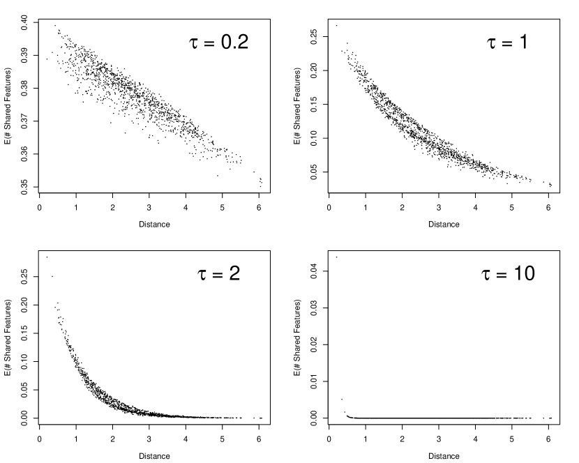
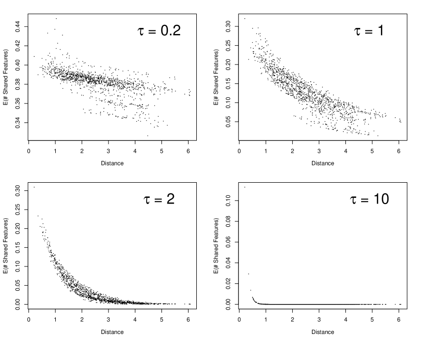
Figure S.1 shows the expected number of shared features between two states as a function of temperature for the dd-IBP with a symmetric proximity matrix. In this case, the permutation is irrelevant because there is no ordering of the customers. As shown, the expected number of shared features has an initial increase and then decreases as the temperature parameter increases. Across all pairs of states and for all temperatures the amount of sharing is lower than the IBP (dashed line at 0.5). As the temperature goes to infinity the sharing goes to zero.

Figures S.2, S.3, S.4, and S.5 explore the expected pairwise feature sharing for the $50$ states in the USArrests dataset. The plots show the expected shared number of features at four fixed temperatures, where $\alpha=1$, for both the AIBD and the dd-IBP, and when the permutation is averaged out of the model and fixed. As expected, there is a negative correlation in all of the plots. When the temperature is zero all points would be at 0.5 (with the IBP). At the temperature of 0.2 all four scenarios show some change in feature sharing. As the temperature increases the AIBD stays centered around 0.5, but the dd-IBP is driven towards no sharing. Additionally, for both the AIBD and the dd-IBP the scatter of points becomes less diffuse when the permutation is integrated out the model. In all cases of the dd-IBP, all points are below the IBP level of 0.5.

S.4 Posterior Summaries

This section contains the posterior means (and standard deviations in parentheses) of the parameters for the various models from Section 6. The first five rows of Table S.3 contain the results for the AIBD with fixed temperatures. The sixth row is from the AIBD with random temperature and permutation. The seventh row of Table S.3 is the AIBD with random temperature and permutation and using the reciprocal similarity function (all other models use the exponential decay similarity function). Rows 8–12 show the results for the dd-IBP models with fixed temperatures. The last row shows the posterior summaries for the parameters in the IBP model.

	Mass	Temperature	$\sigma_{X}$	$\sigma_{A}$
AIBD (temp$=$0.4)	12.1 (1.6)	0.40 (0.00)	0.52 (0.01)	0.38 (0.01)
AIBD (temp$=$0.8)	12.0 (1.6)	0.80 (0.00)	0.52 (0.01)	0.37 (0.01)
AIBD (temp$=$1.2)	11.8 (1.6)	1.20 (0.00)	0.52 (0.01)	0.37 (0.01)
AIBD (temp$=$1.6)	11.7 (1.6)	1.60 (0.00)	0.52 (0.01)	0.37 (0.01)
AIBD (temp$=$2.0)	11.6 (1.6)	2.00 (0.00)	0.52 (0.01)	0.37 (0.01)
AIBD	13.2 (1.7)	2.77 (0.29)	0.52 (0.01)	0.35 (0.01)
AIBD (recip sim)	12.7 (1.8)	0.22 (0.02)	0.52 (0.01)	0.37 (0.01)
dd-IBP (temp$=$0.4)	6.8 (1.7)	0.40 (0.00)	0.60 (0.03)	0.32 (0.03)
dd-IBP (temp$=$0.8)	5.8 (1.0)	0.80 (0.00)	0.58 (0.02)	0.32 (0.02)
dd-IBP (temp$=$1.2)	4.3 (0.9)	1.20 (0.00)	0.60 (0.02)	0.35 (0.03)
dd-IBP (temp$=$1.6)	5.0 (4.8)	1.60 (0.00)	0.59 (0.03)	0.35 (0.02)
dd-IBP (temp$=$2.0)	4.4 (2.6)	2.00 (0.00)	0.59 (0.03)	0.36 (0.03)
IBP	12.4 (1.6)	–	0.52 (0.01)	0.38 (0.01)

Table S.3: Posterior parameter summaries. The posterior means of the parameters for the various models. The posterior standard deviations are included in parentheses.

References

- Blei and Frazier (2011) Blei, D. M. and Frazier, P. I. (2011). “Distance dependent Chinese restaurant processes.” Journal of Machine Learning Research, 12(Aug): 2461–2488. \bptokaddids\endbibitem
- Chen et al. (2013) Chen, M., Gao, C., and Zhao, H. (2013). “Phylogenetic Indian buffet process: Theory and applications in integrative analysis of cancer genomics.” arXiv preprint https://arxiv.org/abs/1307.8229. \bptokaddids\endbibitem
- Dahl et al. (2017) Dahl, D. B., Day, R., and Tsai, J. W. (2017). “Random partition distribution indexed by pairwise information.” Journal of the American Statistical Association, 112(518): 721–732. \bptokaddids\endbibitem
- Dahl et al. (2021) Dahl, D. B., Warr, R. L., Meyer, J. M., and Lui, A. (2021). aibd: Attraction Indian Buffet Distribution. R package version 0.1.9. URL https://CRAN.R-project.org/package=aibd. \bptokaddids\endbibitem
- Dinov et al. (2009) Dinov, I., Van Horn, J., Lozev, K., Magsipoc, R., Petrosyan, P., Liu, Z., MacKenzie-Graha, A., Eggert, P., Parker, D. S., and Toga, A. W. (2009). “Efficient, distributed and interactive neuroimaging data analysis using the LONI pipeline.” Frontiers in neuroinformatics, 3: 22. \bptokaddids\endbibitem
- Doshi et al. (2009) Doshi, F., Miller, K., Gael, J. V., and Teh, Y. W. (2009). “Variational inference for the Indian buffet process.” In van Dyk, D. and Welling, M. (eds.), Proceedings of the Twelth International Conference on Artificial Intelligence and Statistics, volume 5 of Proceedings of Machine Learning Research, 137–144. Hilton Clearwater Beach Resort, Clearwater Beach, Florida USA: PMLR. URL http://proceedings.mlr.press/v5/doshi09a.html. \bptokaddids\endbibitem
- Gelman et al. (2013) Gelman, A., Carlin, J. B., Stern, H. S., Dunson, D. B., Vehtari, A., and Rubin, D. B. (2013). Bayesian data analysis. CRC press, 3 edition. \bptokaddids\endbibitem
- Gershman (2013) Gershman, S. J. (2013). “Matlab code for the distance dependent infinite latent feature models article.” URL http://gershmanlab.webfactional.com/pubs/ddIBP_release.zip. Accessed: 2017-11-15. \bptokaddids\endbibitem
- Gershman et al. (2015) Gershman, S. J., Frazier, P. I., and Blei, D. M. (2015). “Distance dependent infinite latent feature models.” IEEE Transactions on Pattern Analysis and Machine Intelligence, 37(2): 334–345. \bptokaddids\endbibitem
- Goeman (2010) Goeman, J. J. (2010). “L1 penalized estimation in the Cox proportional hazards model.” Biometrical Journal, 1(52): 70–84. \bptokaddids\endbibitem
- Goeman et al. (2018) Goeman, J. J., Meijer, R. J., and Chaturvedi, N. (2018). Penalized: L1 (lasso and fused lasso) and L2 (ridge) penalized estimation in GLMs and in the Cox model. R package version 0.9-51. \bptokaddids\endbibitem
- Griffiths and Ghahramani (2005) Griffiths, T. L. and Ghahramani, Z. (2005). “Infinite latent feature models and the Indian buffet process.” Technical Report 2005-001, Gatsby Computational Neuroscience Unit. \bptokaddids\endbibitem
- Griffiths and Ghahramani (2006) Griffiths, T. L. and Ghahramani, Z. (2006). “Infinite latent feature models and the Indian buffet process.” In Advances in neural information processing systems, 18, 475–482. Cambridge, MA: MIT Press. \bptokaddids\endbibitem
- Griffiths and Ghahramani (2011) Griffiths, T. L. and Ghahramani, Z. (2011). “The Indian buffet process: An introduction and review.” Journal of Machine Learning Research, 12(Apr): 1185–1224. \bptokaddids\endbibitem
- Hai-son and Bar-Joseph (2011) Hai-son, P. L. and Bar-Joseph, Z. (2011). “Inferring interaction networks using the IBP applied to microrna target prediction.” In Advances in Neural Information Processing Systems, 235–243. \bptokaddids\endbibitem
- Lee et al. (2015) Lee, J., Müller, P., Gulukota, K., Ji, Y., et al. (2015). “A Bayesian feature allocation model for tumor heterogeneity.” The Annals of Applied Statistics, 9(2): 621–639. \bptokaddids\endbibitem
- Lee et al. (2016) Lee, J., Müller, P., Sengupta, S., Gulukota, K., and Ji, Y. (2016). “Bayesian inference for intratumour heterogeneity in mutations and copy number variation.” Journal of the Royal Statistical Society: Series C (Applied Statistics), 65(4): 547–563. \bptokaddids\endbibitem
- Lui et al. (2020) Lui, A., Lee, J., Thall, P. F., Daher, M., Rezvani, K., and Barar, R. (2020). “A Bayesian feature allocation model for identification of cell subpopulations using cytometry data.” arXiv preprint https://arxiv.org/abs/2002.08609. \bptokaddids\endbibitem
- Miller et al. (2012) Miller, K. T., Griffiths, T., and Jordan, M. I. (2012). “The phylogenetic Indian buffet process: A non-exchangeable nonparametric prior for latent features.” arXiv preprint https://arxiv.org/abs/1206.3279. \bptokaddids\endbibitem
- Ni et al. (2018) Ni, Y., Mueller, P., and Ji, Y. (2018). “Bayesian double feature allocation for phenotyping with electronic health records.” arXiv preprint https://arxiv.org/abs/1809.08988. \bptokaddids\endbibitem
- Ranganath et al. (2014) Ranganath, R., Gerrish, S., and Blei, D. (2014). “Black box variational inference.” In Kaski, S. and Corander, J. (eds.), Proceedings of the Seventeenth International Conference on Artificial Intelligence and Statistics, volume 33 of Proceedings of Machine Learning Research, 814–822. Reykjavik, Iceland: PMLR. URL http://proceedings.mlr.press/v33/ranganath14.html \bptokaddids\endbibitem
- Sengupta et al. (2014) Sengupta, S., Wang, J., Lee, J., Müller, P., Gulukota, K., Banerjee, A., and Ji, Y. (2014). “Bayclone: Bayesian nonparametric inference of tumor subclones using NGS data.” In Pacific Symposium on Biocomputing Co-Chairs, 467–478. World Scientific. \bptokaddids\endbibitem
- SOCR (2009) SOCR (2009). “SOCR Data July2009 ID NI.” URL http://wiki.stat.ucla.edu/socr/index.php/SOCR_Data_July2009_ID_NI. Accessed: 2019-04-15. \bptokaddids\endbibitem
- Tan et al. (2018) Tan, X., Rao, V., and Neville, J. (2018). “The Indian buffet Hawkes process to model evolving latent influences.” In Conference on Uncertainty in Artificial Intelligence (UAI), 795–804. \bptokaddids\endbibitem
- Teh et al. (2007) Teh, Y. W., Grür, D., and Ghahramani, Z. (2007). “Stick-breaking construction for the Indian buffet process.” In Meila, M. and Shen, X. (eds.), Proceedings of the Eleventh International Conference on Artificial Intelligence and Statistics, volume 2 of Proceedings of Machine Learning Research, 556–563. San Juan, Puerto Rico: PMLR. URL http://proceedings.mlr.press/v2/teh07a.html \bptokaddids\endbibitem
- Williamson et al. (2010) Williamson, S., Orbanz, P., and Ghahramani, Z. (2010). “Dependent Indian buffet processes.” In Teh, Y. W. and Titterington, M. (eds.), Proceedings of the Thirteenth International Conference on Artificial Intelligence and Statistics, volume 9 of Proceedings of Machine Learning Research, 924–931. Chia Laguna Resort, Sardinia, Italy: PMLR. URL http://proceedings.mlr.press/v9/williamson10a.html \bptokaddids\endbibitem
- Williamson et al. (2020) Williamson, S. A., Zhang, M. M., and Damien, P. (2020). “A new class of time dependent latent factor models with applications.” Journal of Machine Learning Research, 21(27): 1–24. \bptokaddids\endbibitem
- Xu et al. (2013) Xu, Y., Lee, J., Yuan, Y., Mitra, R., Liang, S., Müller, P., and Ji, Y. (2013). “Nonparametric Bayesian bi-clustering for next generation sequencing count data.” Bayesian Analysis, 8(4): 759. \bptokaddids\endbibitem
- Xu et al. (2015) Xu, Y., Müller, P., Yuan, Y., Gulukota, K., and Ji, Y. (2015). “MAD Bayes for tumor heterogeneity—feature allocation with exponential family sampling.” Journal of the American Statistical Association, 110(510): 503–514. \bptokaddids\endbibitem