Complete Realization of Energy Landscape and Non-equilibrium Trapping Dynamics in Spin Glass and Optimization Problem

Abstract

Energy landscapes are high-dimensional surfaces representing the dependence of system energy on variable configurations, which determine crucially the system’s emergent behavior but are difficult to be analyzed due to their high-dimensional nature. In this article, we introduce an approach to reveal the complete energy landscapes of small spin glasses and Boolean satisfiability problems, which also unravels their non-equilibrium dynamics at an arbitrary temperature for an arbitrarily long time. In contrary to our common belief, our results show that it can be less likely to identify the ground states when temperature decreases, due to trapping in individual local minima, which ceases at different time, leading to multiple abrupt jumps with time in the ground-state probability. Simulations agree well with theoretical predictions on these remarkable phenomena. Finally, for large systems, we introduce a variant approach to extract partially the energy landscapes and observe both analytically and in simulations similar phenomena. This work introduces new methodology to unravel the non-equilibrium dynamics of glassy systems, and provides us with a clear, complete and new physical picture on their long-time behaviors inaccessible by modern numerics.

Energy landscapes of physical systems are high-dimensional surfaces representing the dependence of system energy on variable configurations. A similar notion of cost landscapes is defined for optimization problems. Their characteristics determine crucially the emergent behavior of the systems. For instance, spin glasses and ferromagnetic spin systems are believed to be characterized by energy landscapes with and without a large number of local minima respectively [1, 2]; a similar analogy is made with the so-called algorithmic hard and easy phases of combinatorial optimization problems [3]. A way to unravel and analyze the characteristics of a complete energy landscape is thus crucial to our understanding of these glassy systems.

Nevertheless, even for small systems, revealing completely their energy landscapes is difficult since they are high-dimensional functions. Although there are various approaches, some features of the landscapes have to be omitted for a feasible characterization. For instance, disconnectivity graphs (DG) connect attraction basins in the state space and show hierarchically how they are repeatedly segmented into smaller basins as energy decreases [4]. DGs have been applied to analyze energy landscapes of systems from protein folding and spin glasses to machine learning [4, 5, 6], and can be improved using principal component analyses [7]. However, DGs only show the segmentation into basins, without showing their entropy nor how states are exactly connected, especially as basins may have multiple instead of one direct connection to other states. Another common approach is multi-dimensional scaling (MDS), which aims to preserve the high-dimensional distance or similarity between two states in a plot of reduced dimension [8]. For instance, one may preserve the distance between pairs of states in one-dimensional plots [9]. Nevertheless, MDS only shows pairwise distance while dynamics on these systems are definitely more complex than pairwise interactions. All these approaches attempt to characterize energy landscapes by omitting some of their features.

In this article, we introduce an approach to reveal the complete energy landscape of complex disordered systems such as spin glasses and Boolean satisfiability problems. The approach is feasible on small systems, while for large systems, we introduce a variant of the approach to obtain a partial energy landscape. The obtained energy landscapes allow us to compute analytically the non-equilibrium dynamics at an arbitrary temperature for an arbitrary long time, out of reach by simulations limited by modern computational capability. Remarkably, in contrary to our common belief, we show that it can be less likely to identify the ground states when temperature decreases, due to trapping in local minima; as time increases, trapping in individual minima ceases at different time, leading to multiple abrupt jumps in the ground-state probability. Our findings also provide insights on the effectiveness of simulated annealing compared with fixed-temperature dynamics, whereas only an extremely long annealing process that allows an escape from local minima may guarantee a ground state [10]. All in all, our approach opens up a new platform for analyzing the non-equilibrium dynamics of glassy systems, and provides us with a clear, complete and new physical picture on their long-time behaviors inaccessible by existing approaches and numerics.

Models Studied - We consider a system with $N$ Boolean variables $s_{i}=\pm 1$, such that $i=1,\dots,N$ and ${\vec{s}}$ denotes the $N$-tuple $(s_{1},s_{2},\dots,s_{N})$ representing a variable configuration. We then denote the energy or objective function of the system as $E({\vec{s}})$. Here, we examine two glassy systems as examples, namely (i) spin glasses [1] and (ii) $K$-satisfiability problems [11].

For spin glasses, each ${\vec{s}}$ is a configuration of Ising spins and $E({\vec{s}})$ is given by

$$E({\vec{s}})=\frac{1}{2}\sum_{i<j}a_{ij}J_{ij}s_{i}s_{j},$$ (1)

where $J_{ij}=+1$ with a probability $f_{+}$ and otherwise $J_{ij}=-1$; the adjacency matrix $a_{ij}=0,1$ characterizes different graph topologies. We multiply $E$ by a factor of $1/2$, such that a single spin flip leads to a unit change in energy. Depending on the topology, the parameter $f_{+}$ and the temperature, the spin system exhibits various phases such as paramagnetic, ferromagnetic and spin glass phases [1, 12].

For $K$-satisfiability problems, or $K$-Sat for short, we introduce $M$ clauses of the form $(s_{\mu_{1}}\vee\overline{s}_{\mu_{2}}\vee\dots\vee s_{\mu_{K}})$ labeled by $\mu=1,\dots,M$, each with $K$ variables or their negation; the symbol $\vee$ corresponds to the “or” logical relation and the variables with an overline are negated. In this case, $E({\vec{s}})$ is given by

$$E({\vec{s}})=\frac{1}{2^{K}}\sum_{\mu=1}^{M}\prod_{k=1}^{K}(1-J_{\mu,k}s_{\mu_{k}}),$$ (2)

where randomly drawn $J_{\mu,k}=\pm 1$ corresponds to the presence of the original or the negated $k$-th variable in clause $\mu$. With the factor of $\frac{1}{2^{K}}$, each violated clause increases the energy by $1$ and the total energy is equivalent to the number of violated clauses. The ground state of the system is attained when $E=0$, i.e. all clauses are satisfied. Depending on the ratio $\alpha=M/N$, the system exhibits various phases including a satisfiable phase at small $\alpha$ with an algorithmic-easy and -hard regime, followed by an unsatisfiable phase at large $\alpha$ [13].

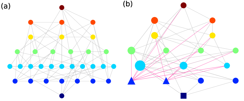
Figure 1: (a) An example of FEL with $2^{N}=32$ configurations from $E=$ at the top to E=0 at the bottom, of a $3$-Sat problem with $N=5$ variables and $\alpha=4$. (b) The corresponding CEL with ${\cal C}=17$ clusters. Global minima and local minima are shown in squares and triangles respectively; node size corresponds to the number of constituent configurations in the clusters; red links correspond to the connections to local minima.

Coarse-grained Energy Landscape (CEL) - Since there are $N$ Boolean variables in the above systems, there are $2^{N}$ different variable configurations. If we consider two configurations ${\vec{s}}_{a}$ and ${\vec{s}}_{b}$ to be connected in the configurational space if their hamming distance is $|{\vec{s}}_{a}-{\vec{s}}_{b}|=1$, i.e. they differ only in the state of a single variable, the configurational space is effectively a $N$-dimensional hypercube.

To present this hypercube as an energy landscape, we take advantage of the integer disorders $J$ defined in the above systems, which lead to discrete energy levels. We then represent each variable configuration ${\vec{s}}$ as a node in a network; two nodes are connected by a link if their hamming distance is 1. Next, we arrange nodes with the same energy on the same horizontal level in the network, with lower-energy configurations located at a lower row. We call this the full energy landscape (FEL). For the sake of clear illustration, we show an example of FEL for a small $3$-Sat toy problem with $N=5$ and $\alpha=4$ in Fig. 1(a). One can see clearly how the $2^{N}=32$ different configurations are connected and arranged at different energy levels. Nevertheless, as $N$ further increases, the number of states increases exponentially and FELs quickly become computational infeasible and difficult to be clearly visualized.

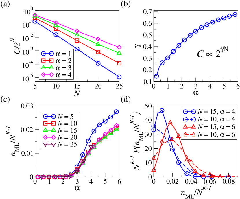
Figure 2: (a) The number of clusters in CEL divided by the number of configurations in FEL, i.e. ${\cal C}/2^{N}$, as a function of $N$. (b) The exponent $\gamma$ in ${\cal C}=2^{\gamma N}$ as a function of $\alpha$ in the $3$-Sat problem. (c) The number of local minima in CEL, rescaled with $N^{2}$ of the $3$-Sat problem as a function of $\alpha$ for different system size $N$.

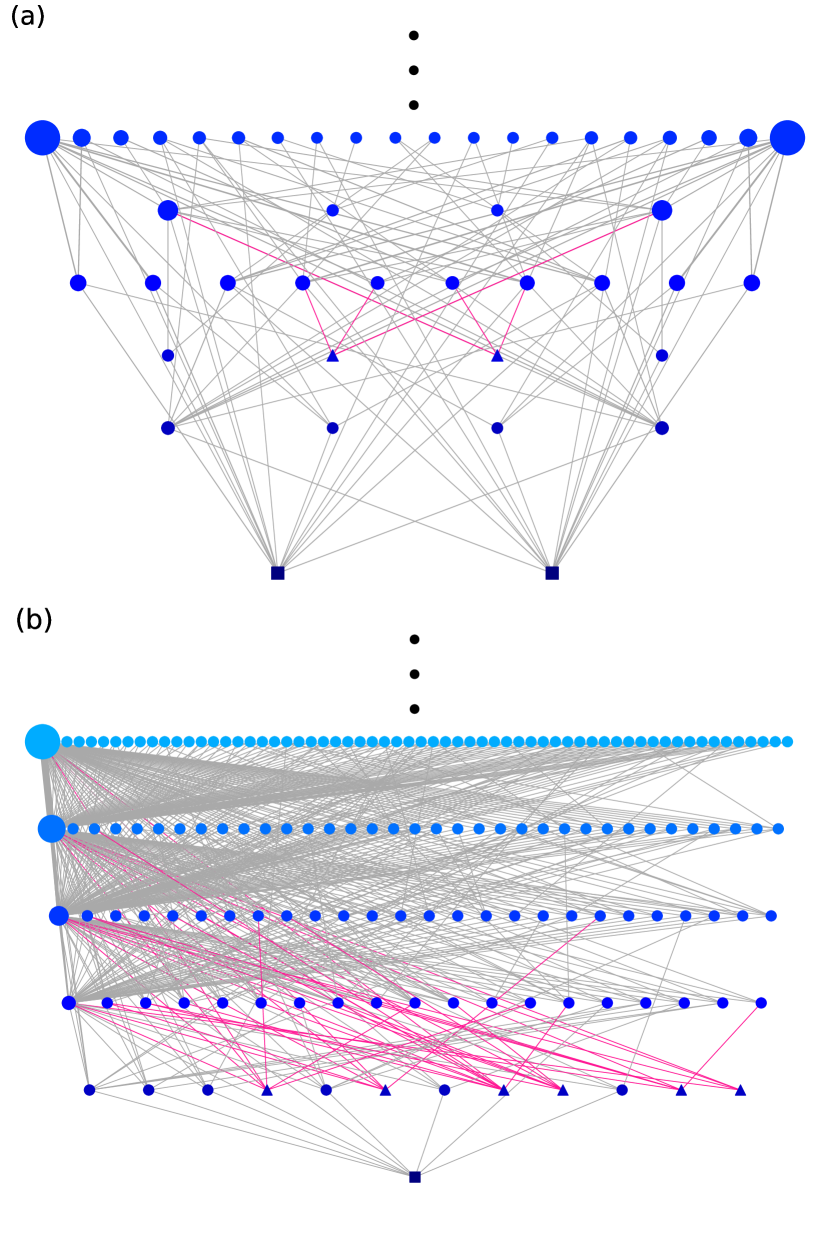
Figure 3: The low-energy portion of examplar CELs for an instance of (a) spin glass on random regular graph with $f_{+}=0.5$ and (b) 3-Sat problem with $\alpha=4$, both with $N=15$. Global minima and local minima are shown in squares and triangles respectively; node size corresponds to the number of constituent configurations in the clusters; red links correspond to the connections to local minima.

To simplify the energy landscape, we group connected nodes on the same energy level into clusters; we denote ${\cal C}$ to be the total number of clusters. Two clusters $a$ and $b$ are connected if any pair of their constituent variable configurations are connected; the weight $w_{ab}$ of the connection is the total number of links between their constituent configurations. We call this energy landscape the coarse-grained energy landscape (CEL). The corresponding CEL of the FEL in Fig. 1(a) is shown in Fig. 1(b), where the number of nodes is reduced from $2^{N}=32$ in FEL to ${\cal C}=17$ in CEL. As shown in Fig. 2(a), as $N$ further increases, the ratio ${\cal C}/2^{N}$ decreases exponentially with $N$, implying that an extensive number of configurations can be grouped in CEL for a clear presentation. This also implies that ${\cal C}\propto 2^{\gamma N}$, with $\gamma<1$. As shown in Fig. 2(b), $\gamma$ increases with $\alpha$, implying that the structure of energy landscape is more complicated at large $\alpha$, consistent with our understanding of algorithmic-hard regimes compared with easy ones at small $\alpha$.

Interestingly, as shown in Fig. S1(a) of the Supplementary Information (SI), the exponent $\gamma$ for $K$-Sat problems with different $K$ and $\alpha$ collapses onto a common function of $\alpha/K^{2}$. This implies that the decrease of nodes by grouping configurations in CEL is universal for different values of $N$, $M$ and $K$, which is further shown by the ratio $({\cal C}/2^{N})^{1/(1-\gamma)}$ collapsed onto a common exponential decay against $N$ in Fig. S1(b).

Other than a large reduction in the number of nodes, another advantage of CEL is the identification of local minima. Since connected configurations with the same energy are grouped in clusters in CELs, one can easily identify local minima as clusters where all neighbors are of higher energy; such identification is not trivial in FEL since it is difficult to examine if there exists a path from a configuration to a lower-energy one without passing through higher-energy configurations. In the CEL in Fig. 1(b), one can see that there exist two local minima (triangles) with $E=1$. We show in Fig. 3 the low-energy portion of another examplar CEL of spin glasses on random regular graphs (RRG) with $N=15$ and $f_{+}=0.5$; since the configurations ${\vec{s}}$ and $-{\vec{s}}$ have the same energy according to Eq. (1), one can observe a symmetric structure in the energy landscape as expected, including a pair of local minima at $E=3$. Another example of CEL for $3$-Sat problem with $N=15$ and $\alpha=4$ is shown in Fig. 3(b), where six local minima are found at $E=1$. More examplar CELs of systems with larger $N$ are found in Fig. S2 of the SI.

CELs thus allow us to obtain the statistics of local minima, and the number of local minima $n_{\rm LM}$ is shown as a function of $\alpha$ for the $3$-Sat problem in Fig. 2(c). As we can see, local minima start to emerge beyond $\alpha\gtrsim 2.5$ and increase with $\alpha$. This is again consistent with the phenomenon of increasing algorithmic hardness as $\alpha$ increases. Interestingly, $n_{\rm LM}$ scales with $N^{K-1}$, which may imply that the emergence of local minima is related to the number of possible constraints per variable. We further show the distribution of $n_{\rm LM}/N^{K-1}$ in Fig. 2(d), where the distributions become narrower as $N$ increases. We remark that these results are different from most of the previous exhaustic studies on small combinatorial systems which mainly focus on ground states [14].

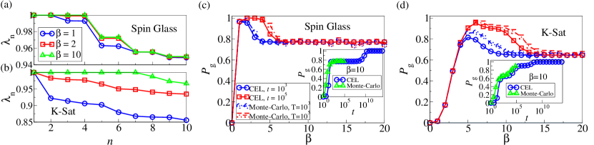
Figure 4: (a,b) The first ten largest eigenvalues, i.e. $\lambda_{n}(\beta)$ with $n=1,\dots,10$, of the transition matrix ${\cal T}_{\beta}$ at $\beta=1,2,10$, for the examplar spin glass and 3-Sat problem instances of which CELs are shown in Fig. 3(a) and (b) respectively. (c,d) The probability ${P_{g}}$ of finding the ground states of the examplar spin glass and 3-Sat problem instances as a function of inverse-temperature $\beta$ obtained by Eq. (4) after $t=10^{3}$ and $10^{5}$ iterations, compared with simulation results. Insets: ${P_{g}}$ as a function of time $t$.

Trapping Dynamics - Thanks to the largely reduced number of nodes and the identification of local minima in CELs, they allow us to reveal the complete non-equilibrium dynamics when these glassy systems are trapped in local minima, at an arbitrary temperature for an arbitrarily long time. Here, one can formulate a matrix of transition probabilities $T_{a\to b}$ from a cluster $a$ to $b$, describing the Metropolis-Hasting (Markov Chain Monte Carlo (MCMC)) dynamics of the system following the Boltzmann distribution [15, 16]. In this case, $T_{a\to b}$ for $a\neq b$ is given by

$$T_{a\to b}(\beta)=\frac{w_{ab}}{n_{a}N}\frac{e^{-\beta\Delta E_{a\to b}}}{e^{-\beta\Delta E_{a\to b}}+1}$$ (3)

where $\Delta E_{a\to b}=E_{b}-E_{a}$ and $\beta$ is the inverse-temperature; $n_{a}$ corresponds to the size of cluster $a$, and $n_{a}N$ corresponds to the total number of links connecting its constituent configurations, including those internal links within cluster $a$. On the other hand, for the system to stay in cluster $a$, the system can either reject the transition to a configuration outside $a$ or transit to another configuration within $a$, with a total probability given by $T_{a\to a}(\beta)=1-\sum_{b\neq a}T_{a\to b}(\beta)$. We then denote the probabilities to find the system in configurations in individual clusters at time $t$ by a vector ${\vec{P}}_{t}=(P_{1},\dots,P_{\cal C})$, and express

$${\vec{P}}_{t}={\cal T}_{\beta}{\vec{P}}_{t-1}={\cal T}_{\beta}^{t}{\vec{P}}_{0},$$ (4)

where ${\cal T}_{\beta}$ is the transition matrix with element $T_{a\to b}(\beta)$.

With the matrix ${\cal T}_{\beta}$ for specific instances, one can conduct a spectral analysis to compute its eigenvalues. We first denote $\lambda_{n}(\beta)$ to be the $n$-th largest eigenvalue of ${\cal T}_{\beta}$. We show in Fig. 4(a) and (b) $\lambda_{1}$ to $\lambda_{10}$ at different inverse-temperatures $\beta$ for the spin glass and $K$-Sat instances shown in Fig. 3(a) and (b) respectively. We first note that the eigenvalues of the spin glass instance are in pairs due to the symmetric nature of its energy landscape. More interestingly, $\lambda_{n}$ differ more at small $\beta$, but the few eigenvalues after $\lambda_{1}$ start to approach 1 as $\beta$ increases. The number of eigenvalues approaching 1 is equal to the number of local minima in the corresponding CELs, i.e. $\lambda_{3}$ and $\lambda_{4}$ of the spin glass instances correspond to the two symmetric local minima in Fig. 3(a) and $\lambda_{2}$ to $\lambda_{7}$ of the $3$-Sat instance correspond to the six local minima with $E=1$ n Fig. 3(b). The increasing proximity of these eigenvalues to 1 also corresponds to an increasing trapping in local minima when $\beta$ increases, comparable to the trapping in global minima with $\lambda_{1}=1$. This also raises a question on whether the systems equilibrate at the ground states at zero temperature (i.e. $\beta\to\infty$), since $\lambda_{n}\to 1$ for the local minima and are equivalent to $\lambda_{1}=1$ at the ground states.

Since we can obtain the complete transition matrix for these small systems through CELs, one can compute their complete dynamics at an arbitrary temperature for an arbitrarily long time using Eq. (4). Starting with a uniform ${\vec{P}}_{0}$, we show the probability ${P_{g}}$ of the spin glass and the $3$-Sat instances being in the ground state after $t=10^{3}$ and $10^{5}$ iteration steps as a function of $\beta$ in Fig. 4(c) and (d). As we can see, for both instances ${P_{g}}$ first increases with $\beta$ as expected, but remarkably decreases as $\beta$ further increases; the MCMC simulation results are in good agreement with these theoretical predictions by CELs. These results imply that with a random initial condition, the trapping at local minima becomes more significant as temperature decreases below some specific values and it is less likely to locate the ground states within a finite time.

As we can see, time $t$ seems to play an important role as the optimal range of $\beta$ with high ${P_{g}}$ widens with $t$. We further show in the insets of Fig. 4(c) and (d) that ${P_{g}}$ increases with $t$. Nevertheless, the increase is not smooth and multiple jumps and plateaus are observed, implying that local minima are completing with the global minima for the probability but they cease to trap the system at different time $t$. This phenomenon can be explained by eigenvalues, where a sufficiently large $t$ makes $\lambda_{n}^{t}$ of the local minima sufficiently less than 1, despite $\lambda_{n}\approx 1$ (see again Fig. 4(a) and (b)). This also implies that the proximity of $\lambda_{n}$ to 1 is related to the ability or stiffness of individual minima in trapping the system, which may depend on their entropy or number of external connections; one may thus estimate the characteristic duration of trapping in individual minima using $\lambda_{n}$.

We remark that MCMC simulations are in good agreement with theoretical predictions, including the drop in ${P_{g}}$ with $\beta$ and the abrupt jumps and plateaus of ${P_{g}}$ at small $t$, while the small discrepancies may come from the mean-field nature of the clustered transition probabilities in Eq. (4). In addition, since one can easily compute ${\cal T}_{\beta}^{t}$ for an arbitrarily large $t$, e.g. $10^{14}$ in the insets of Fig. 4(c) and (d), by repeatedly powering ${\cal T}_{\beta}^{t}$ and its products, one can obtain the long-time dynamics by Eq. (4) out of reach by modern computational capability. For the sake of a clear illustration and elaboration, we show the above results for only two instances; in Fig. S3 of the SI, we show that the sample-averaged ${P_{g}}$ exhibits a similar behavior against $\beta$ and $t$. Sample-averaged MCMC simulation results are also in good agreement with theoretical predictions.

Implications on Simulated Annealing - The eigenvalues of the transition matrix ${\cal T}_{\beta}$ from CELs also provide implications on the essence of cooling in simulated annealing (SA). As we see from Fig. 4(a) and (b), the difference among eigenvalues is large at small $\beta$ when the system can distinguish $\lambda_{1}$ of the global minima from $\lambda_{n}$ of local minima. With random initial conditions, eigenvalues are getting closer in values as $\beta$ increases. By cooling the system from a high temperature in SA, the system does not start with a random state at the beginning of each cooling stage but instead continuously biases towards the global minima due to difference between its $\lambda_{1}$ from other $\lambda_{n}$, though this difference is vanishing. This suggests that SA is more effective in identifying ground states compared with fixed-temperature dynamics. Nevertheless, once the system is trapped in a local minimum, lowering temperature in SA does not help the system escape from the minimum, and only an extremely slow (and potentially infeasible) cooling schedule may help.

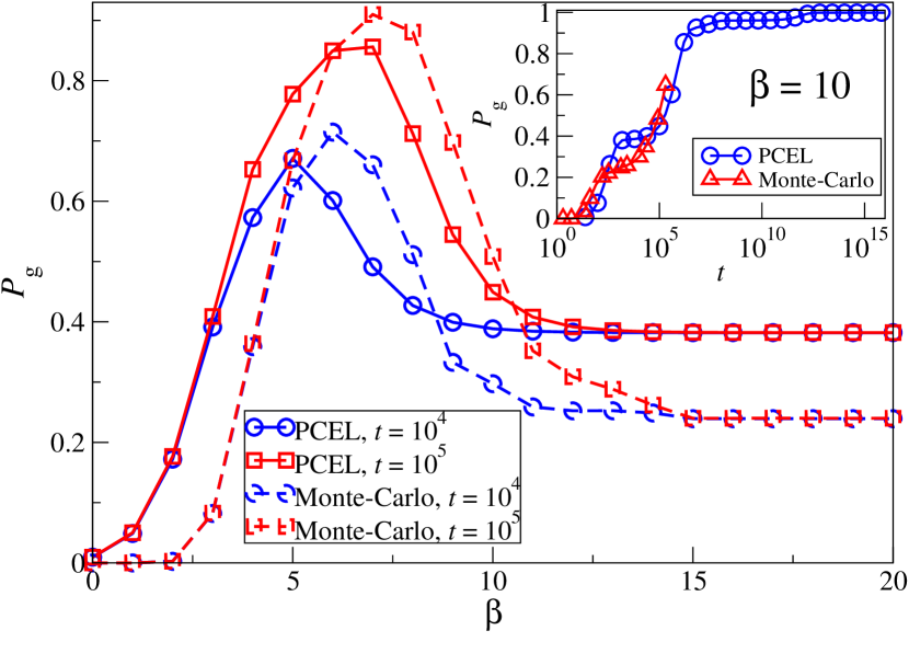
Figure 5: The probability ${P_{g}}$ for a $3$-Sat problem instance with $N=50$ of which PCELs are shown in Fig. S4, as a function of $\beta$, obtained by the transition matrix from PCELs sampled for $T=10^{5}$ steps at ${\beta_{s}}=5$ with $10$ re-starts, and then by Eq. (4) after $t=10^{4}$ and $10^{5}$ iterations, compared with simulation results. Insets: ${P_{g}}$ as a function of time $t$, where a factor of $\ln[2^{N}/n({\vec{s}}_{\rm sampled})]$ has been multiplied to $t$ in the results obtained by PCELs since only part of the energy landscape is extracted, with $n({\vec{s}}_{\rm sampled})$ to be the number of sampled configurations.

Partial Coarse-grained Energy Landscape (PCEL) - The computation of CELs is only feasible for systems with small size $N$ since it requires examining all $2^{N}$ variable configurations. Nevertheless, for large systems, we introduce a method to obtain a partial coarse-grained energy landscape (PCEL) for the low-energy configurations. In this case, we sample variable configurations by MCMC simulations at a fixed sampling inverse-temperature ${\beta_{s}}$ for $T$ steps, and restart the sampling with random initial conditions for multiple times. We record all the sampled configurations for the construction of PCELs following the same procedures as in CELs. By using an appropriate ${\beta_{s}}$, one can extract specific part of the energy landscape, for instance, a moderately large ${\beta_{s}}$ for extracting the low-energy configurations.

We remark that PCELs are only approximations since MCMC simulations with finite time $T$ can only sample a small fraction of all $2^{N}$ configurations, though the number of sampled configurations for systems with large $N$ can be significantly larger than those of the small systems we presented before. In addition, it can happen that clusters with the same energy in PCELs indeed belong to a larger cluster since not all the intermediate configurations between the two clusters are sampled. An example of PCEL for a $K$-Sat problem with $N=50$ is shown in Fig. S4(a) of the SI. Since we are mainly interested in the glassy behaviors contributed by the global and local minima, to further simplify the analyses, we make one more approximation to leave only a single shortest path between minima in PCELs to obtain a simplified transition matrix $\tilde{\cal T}_{\beta}$; the simplified version of PCEL in Fig. S4(a) is shown in Fig. S4(b). We found that the results obtained by the simplified $\tilde{\cal T}_{\beta}$ are similar to those without this simplification.

The major advantage in using PCELs to analyze system dynamics is that a single MCMC procedure to extract the PCEL at a single ${\beta_{s}}$ can provide us with the dynamics of the system at an arbitrary temperature for an arbitrarily long time out of which by simulations. We show the dynamics of a $3$-Sat problem with $N=50$ in Fig. 5, which is obtained by the simplified PCEL shown in Fig. S4(b) sampled at a single ${\beta_{s}}=5$. The theoretical results agree well with simulations at different $\beta$ except those at small $\beta$ when the system explores high-energy configurations while PCELs focus on low-energy configurations. The corresponding sampled-averaged plot is shown in Fig. S5. The same phenomena as in the small systems are observed, namely the drop in ${P_{g}}$ as temperature decreases, as well as the jumps in ${P_{g}}$ as time $t$ increases. These results suggest that the findings based on CELs in small systems are also observed in large systems, which show that CELs and PCELs open up a new platform for us to reveal the long-time non-equilibrium dynamics for glassy systems.

Summary - We introduced an approach called Coarse-grained Energy Landscape (CEL) to reveal the complete energy landscapes of small glassy systems. In terms of advances in methodology, by formulating CELs and analyzing their transition matrix, one can analytically compute the non-equilibrium dynamics of a system at an arbitrary temperature for an arbitrary long time, out of reach by simulations limited by modern computational capability. For large systems, we introduce a variant of the approach to partially reveal the energy landscapes, which allow us to conduct the same analysis as in small systems. In terms of improved understanding, we show a clear and complete physical picture on how glassy systems are trapped in local minima, as evident from the drop in the ground-state probability as temperature decreases as well as their abrupt jumps as time increases. Simulation results agree well with theoretical predictions. Our work advances methodology by a new tool for analyzing the non-equilibrium dynamics of complex disordered systems, which generate clear, complete and new understandings and insights on their long-time behavior inaccessible by modern numerics.

- [1] Mézard, M., Parisi, G. & Virasoro, M. A. Spin glass theory and beyond: An Introduction to the Replica Method and Its Applications, vol. 9 (World Scientific Publishing Company, 1987).
- [2] Nishimori, H. Statistical physics of spin glasses and information processing: an introduction. 111 (Clarendon Press, 2001).
- [3] Krzakała, F., Montanari, A., Ricci-Tersenghi, F., Semerjian, G. & Zdeborová, L. Gibbs states and the set of solutions of random constraint satisfaction problems. Proceedings of the National Academy of Sciences 104, 10318–10323 (2007).
- [4] Becker, O. M. & Karplus, M. The topology of multidimensional potential energy surfaces: Theory and application to peptide structure and kinetics. The Journal of chemical physics 106, 1495–1517 (1997).
- [5] Zhou, Q. & Wong, W. H. Energy landscape of a spin-glass model: exploration and characterization. Physical Review E 79, 051117 (2009).
- [6] Ballard, A. J. et al. Energy landscapes for machine learning. Physical Chemistry Chemical Physics 19, 12585–12603 (2017).
- [7] Komatsuzaki, T. et al. How many dimensions are required to approximate the potential energy landscape of a model protein? The Journal of chemical physics 122, 084714 (2005).
- [8] Mead, A. Review of the development of multidimensional scaling methods. Journal of the Royal Statistical Society: Series D (The Statistician) 41, 27–39 (1992).
- [9] Heuer, A. Properties of a glass-forming system as derived from its potential energy landscape. Physical review letters 78, 4051 (1997).
- [10] Bertsimas, D., Tsitsiklis, J. et al. Simulated annealing. Statistical science 8, 10–15 (1993).
- [11] Malik, S. & Zhang, L. Boolean satisfiability from theoretical hardness to practical success. Communications of the ACM 52, 76–82 (2009).
- [12] Sherrington, D. & Kirkpatrick, S. Solvable model of a spin-glass. Physical review letters 35, 1792 (1975).
- [13] Mézard, M. & Zecchina, R. Random k-satisfiability problem: From an analytic solution to an efficient algorithm. Physical Review E 66, 056126 (2002).
- [14] Ardelius, J. & Zdeborová, L. Exhaustive enumeration unveils clustering and freezing in the random 3-satisfiability problem. Physical Review E 78, 040101 (2008).
- [15] Metropolis, N., Rosenbluth, A. W., Rosenbluth, M. N., Teller, A. H. & Teller, E. Equation of state calculations by fast computing machines. The journal of chemical physics 21, 1087–1092 (1953).
- [16] Hastings, W. K. Monte carlo sampling methods using markov chains and their applications (1970).