Higher cup products on hypercubic lattices: application to lattice models of topological phases

Abstract

In this paper, we derive the explicit formula for higher cup products on hypercubic lattices, based on the recently developed geometrical interpretation on the simplicial complexes. We illustrate how this formalism can elucidate lattice constructions on hypercubic lattices for various models and deriving them from spacetime actions. In particular, we demonstrate explicitly that the (3+1)D SPT $S=\frac{1}{2}\int w_{2}^{2}+w_{1}^{4}$ (where $w_{1}$ and $w_{2}$ are the first and second Stiefel-Whitney classes) is dual to the 3-fermion Walker-Wang model constructed on the cubic lattice. Other examples include the double-semion model, and also the “fermionic” toric code in arbitrary dimensions on hypercubic lattices. In addition, we extend previous constructions of exact boson-fermion dualities and the Gu-Wen Grassmann Integral to arbitrary dimensions. Another result which may be of independent interest is a derivation of a cochain-level action for the generalized double-semion model, reproducing a recently derived action on the cohomology level.

I Introduction

In algebraic topology, the cup product and higher cup products are fundamental operations on cocycles and cohomology. Cup products defined on simplicial complexes were central to the early development of algebraic topology, and the higher cup products and Steenrod operations introduced in [S47] have also been valuable tools for topologists. These operations were shortly afterwards interpreted geometrically [thom1950] in terms of Poincaré duals of cohomology classes. While these operations have been central to the cohomology-level understanding of topology, cochain-level formulas on concrete simplicial complexes have often been considered opaque and unnecessary for the study of manifold topology. However, renewed interest in these cochain-level formulas has come from the physics community in the study of topological phases of matter. In particular, Gu-Wen [guWen2014Supercohomology] found that cochain-level formulas for higher-cup products and Steenrod squares pop out of fermionic path integral constructions of topological lattice models. And recently, geometric interpretations [T18, T20] of the cochain-level formulas have been found and related to combinatorial spin structures and fermions.

In this paper, we extend the construction of [T20] to the hypercubic lattice and define cochain-level formulas for the higher cup operations on hypercubic lattices. We then apply these formulas and give an expository account through the hypercubic lattice of how they can be used to systematically derive Hamiltonians of some well-known lattice models of topological phases given cochain-level formulas of space-time partition functions of topological actions.

The organization of this paper can roughly be split into two parts; the first half Secs. III-V introduces our operations, while the second half Secs. VI-VII applies the operations to various physical models.

In Section II, we review the simplicial higher cup operations and some previous partial results for conventions in the two- and three-dimensional cubical cases. In Sec. III, we establish convenient notation for the hypercubic cell structures that we use throughout and define chains and cochains. In Sec. IV, we give systematic definitions of the operations in all dimensions over $\mathbb{Z}_{2}$. In Sec. V, we do the same over $\mathbb{Z}$. Here, we find that various sign factors that show up over $\mathbb{Z}$ have interpretations in terms of signed intersections of dual cells.

In Sec. VI, we discuss applications of our formalism to fermionic systems in hypercubic lattices of arbitrary dimensions. In particular, we extend the $d$-dimensional exact boson-fermion duality [chen2020BosonArbDimensions] and the Gu-Wen Grassmann Integral [guWen2014Supercohomology] in $d$-dimensions to the hypercubic case. In Sec. VII, we illustrate how to systematically construct Hamiltonian models of topological phases from topological actions in our hypercubic formalism. Particular examples include the $\mathbb{Z}_{n}$ toric code in arbitrary dimensions, the double-semion model [levinGu2012], the 3-fermion Walker-Wang model [BCFV14], and fermionic toric code [kapustinThorngren2017, chen2020BosonArbDimensions]. On the 3-fermion Walker-Wang model, we briefly discuss how our formalism can simplify the recently-constructed Quantum Cellular Automaton (QCA) [HFH18] . Details are deferred to a future work [myfuturework].

Many detailed and technical calculations are relegated to the appendices. However, Appendix LABEL:app:cochainActionGenDoubleSemion may be of independent interest from the main threads of this paper; there we consider the generalized double-semion model [FH16] and give a cochain-level derivation of the topological action [debray2019] that describes it.

II Review of $\cup_{i}$ products on triangulations and previous conventions on a cubic lattice

First, we review some concepts in algebraic topology and also introduce notations used in this paper, in particular reviewing notation of triangulations and previous constructions of hypercubic cochain operations.

We will always work with an arbitrary triangulation of a simply-connected $d$-dimensional triangulation manifold $M^{d}$ equipped with a branching structure. A branching structure is an assignment of arrows to each $1$-simplex that doesn’t form any closed loops on triangles. This is equivalent to there being a total order on vertices of a $d$-simplex. In general, we’ll write $\Delta_{k}=\braket{0\cdots k}$ so that the branching structure locally orders edges as $0\to\cdots\to k$. We often refer to vertices, edges, faces, and tetrahedra as $v,e,f,t$, respectively. A general $k$-simplex is denoted as $\Delta_{k}$, and we refer to $T^{k}(M^{d})$ as the set of $k$-simplices of $M^{d}$.

Associated to the set of $k$-simplices of $M^{d}$ is the chain space $C_{k}(M^{d},\mathbb{Z})$ which is a free $\mathbb{Z}$-module generated by basis vectors $\{\ket{0\cdots k}\}_{\braket{0\cdots k}\in T^{k}(M^{d})}$. A finite linear combination of $k$-simplices with coefficients in $\mathbb{Z}$ is called a $k$-chain. The $k$-chains form an abelian group denoted $C_{k}(M^{d},\mathbb{Z})$. One can also consider the reductions of these space modulo 2 to give the $\mathbb{Z}_{2}$ chain spaces $C_{k}(M^{d},\mathbb{Z}_{2})$. A $\mathbb{Z}_{2}$-valued $k$-chain can be identified with a finite set of $k$-simplices (the set consisting of those simplices whose coefficients are nonzero).

Now we define cochains, over $\mathbb{Z}_{2}$. A $\mathbb{Z}_{2}$-valued $k$-cochain is a function from the set of $k$-simplices to $\mathbb{Z}_{2}$, and can be expressed in terms of the dual vectors $\{\bra{0\cdots k}\}_{\braket{0\cdots k}\in T^{k}(M^{d})}$. The set of all $k$-cochains is an abelian group denoted $C^{k}(M^{d},\mathbb{Z}_{2})$. For example, a $0$-cochain assigns an element of $\{0,1\}\in\mathbb{Z}_{2}$ to all vertices, and a $1$-cochain assigns $0$ or $1$ to all edges. A $k$-cochain acts on $k$-chain by evaluating the cochain on each simplex of the $k$-chain and adding up the results modulo $2$. This gives the chain-cochain pairing. For $a\in C_{k}(M^{d},\mathbb{Z}_{2})$ and $b\in C^{k}(M^{d},\mathbb{Z}_{2})$, we often use the notations

$$\int_{M}(a)(b)=\int_{M}(b)(a)=\int_{a}b$$ (2)

to denote this pairing.

For each simplex $\Delta_{k}$, it’s useful to define the indicator cochain ${\bf\Delta}_{k}$. For example, a vertex $v$ is associated to a 0-cochain ${\bf v}$, which takes value $1$ on $v$, and $0$ otherwise, i.e. ${\bf v}(v^{\prime})=\delta_{v,v^{\prime}}$. Similarly, edges $e$ give us 1-cochains ${\bf e}$ with ${\bf e}(e^{\prime})=\delta_{e,e^{\prime}}$, and so forth, i.e., ${\bf f}(f)=\delta_{f,f^{\prime}}$ for the face $f$ . All such indicator cochains will be denoted in bold.

The boundary operator is denoted by $\partial$. For a $k$-simplex $\Delta_{k}=\braket{0\cdots k}$, $\partial\Delta_{k}$ consists of all boundary $(k-1)$-simplices of $\Delta_{k}$. In other words,

$$\partial\ket{0\cdots k}=\sum_{i=0}^{k}\ket{0\cdots\hat{i}\cdots k}$$ (3)

where $\hat{i}$ means skipping over that index.

The coboundary operator $\delta$ (not to be confused with the previous Kronecker delta) acts on cochains and is the the adjoint of $\partial$. On indicator cochains, we’ll have

$$\delta{\bf\Delta}_{k}=\sum_{\Delta_{k+1}\supset\Delta_{k}}{\bf\Delta}_{k+1}.$$ (4)

where the notation $\Delta_{k+1}\supset\Delta_{k}$ means that $\Delta_{k}$ is a subsimplex of $\Delta_{k+1}$. For general cochains, the definition above extends by linearity to give

$$\delta\alpha=\sum_{\Delta_{k}\in\alpha}\sum_{\Delta_{k+1}\supset\Delta_{k}}{\bf\Delta}_{k+1}.$$ (5)

Now, we review product operations over cochains on triangulations. These constructions require a branching structure on the triangulation in order to determine local vertex orderings, whereas the boundary operators did not.

The cup product $\cup\equiv\cup_{0}$ and the higher cup product $\cup_{n}$ were orignally defined by Steenrod [S47] for an arbitrary simplicial complex, and interpreted geometrically in [T18, T20]. In Ref. [CKR18, CK18], similar definitions for $\cup$ and $\cup_{1}$ were given for 2D square lattices and 3D cubic lattices. Here, we’ll review previous definitions on both a triangulated lattice and the cubic lattices and how they fit into the framework of the geometric interpretations.

On a triangulated space, the cup product $\cup$ of a $p$-cochain $\alpha_{p}$ and a $q$-cochain $\beta_{q}$ is a $(p+q)$-cochain defined as [H00]:

$$\begin{split}(\alpha_{p}\cup\beta_{q})(0,\dots,p+q)&=\alpha_{p}(0,1,\dots,p)\beta_{q}(p,p+1,\dots,p+q)\\ &=\alpha_{p}(0\to p)\beta_{q}(p\to p+q).\end{split}$$ (6)

where $i\to j=\{i,i+1,\cdots,j-1,j\}$ are the integers between $i$ and $j$. The cup product satisfies the important Leibniz rule:

$$\delta(\alpha\cup\beta)=\delta\alpha\cup\beta+\alpha\cup\delta\beta.$$ (7)

The $\cup_{m}$ product of a $p$-cochain with a $q$-cochain is a $(p+q-m)$-cochain defined as

$$(\alpha_{p}\cup_{m}\beta_{q})(0,1,\cdots,p+q-m)=\sum_{0\leq i_{0}<i_{1}<\cdots<i_{m}\leq p+q-m}\alpha_{p}(0\to i_{0},i_{1}\to i_{2},i_{3}\to i_{4},\cdots)\beta_{q}(i_{0}\to i_{1},i_{2}\to i_{3},\cdots)$$ (8)

where $\{i_{0},i_{1},\dots,i_{m}\}$ are chosen such that the arguments of $\alpha_{p}$ and $\beta_{q}$ contain $p+1$ and $q+1$ numbers separately. For example,

$$(\alpha_{2}\cup_{1}\beta_{2})(0123)=\alpha_{2}(013)\beta_{2}(123)+\alpha_{2}(023)\beta_{2}(012).$$ (9)

For arbitrary $\mathbb{Z}_{2}$-cochains $\alpha$ and $\beta$, the higher cup products satisfy a recursive Leibniz-like identity.

$$\delta(\alpha\cup_{m}\beta)=\delta\alpha\cup_{m}\beta+\alpha\cup_{m-1}\delta\beta+\alpha\cup_{m}\beta+\beta\cup_{m-1}\alpha.$$ (10)

which agrees with the $\cup_{0}\equiv\cup$ rule setting $\cup_{-1}\equiv 0$.

Now, we describe the geometric interpretations. A $p$-cochain $\alpha$ in $M^{d}$ can be thought of as some $(d-p)$-dimensional surface $\alpha^{\vee}$ living on the dual cellulation. On the cohomology-level, it’s well-known that for closed cochains, $\alpha\cup\beta$ is Poincaré-dual to the intersection of the dual submanifold $\alpha^{\vee}\cap\beta^{\vee}$. However, the formula above actually describes a certain cochain-level intersection between $\alpha^{\vee},\beta^{\vee}$. In order to define an intersection between $\alpha^{\vee},\beta^{\vee}$, one first needs to consider a shifted version of the dual cellulation and also the dual submanifold $\beta^{\vee}_{\text{shifted}}$, where the shifting is determined by a vector field associated to the triangulation. Then, $\alpha\cup\beta$ is dual to $\lim_{\epsilon\to 0}\alpha^{\vee}\cap\beta^{\vee}_{\text{shifted}}$, where $\epsilon$ is some parameter determining the shifting. In Fig. 1, we illustrate this in two dimensions, and give a similar picture that corresponds to a previous $\cup_{0}$ definition on the square lattice, which can be interpreted by resolving the square lattice into a certain branched triangulated lattice.

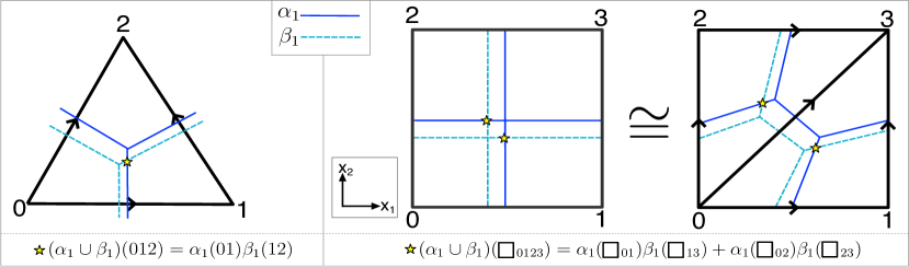
Figure 1: The $\cup$ product between $\alpha$ and $\beta$ can be interpreted as measuring the intersection of $\alpha^{\vee}$ with a shifted version of $\beta^{\vee}$. This can be used to define $\cup$ on a square lattice by resolving the square lattice into a triangular one.

The $\cup_{m}$ products are similar, except instead one considers a thickened intersection product. In particular, one first thickens $\beta^{\vee}$ along $m$ vector fields and shifts along an $(m+1)^{th}$. Then, $\alpha\cup_{m}\beta$ is dual to $\lim_{\epsilon\to 0}\alpha^{\vee}\cap\beta^{\vee}_{\text{thickened,shifted}}$. Another way to think about this thickening is to instead locally project away the thickening direction and measure the intersections in the projected version. This projection was indeed related to the previous definition [CK18] of $\cup_{1}$ on a cubic lattice. This interpretation via a projection is depicted in Fig. 2.

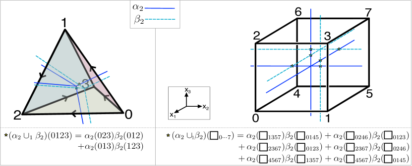
Figure 2: The $\cup_{1}$ product between $\alpha_{2}$ and $\beta_{2}$ in three dimensions can be interpreted measuring the intersections between the cochains in $\alpha_{2}$ on the dual 1-skeleton and $\beta_{2}$ on a shifted dual 1-skeleton after a certain projection onto 2D. Equivalently, it can be thought of as a thickened intersection, where on thickens $\beta$ in precisely the projection direction mentioned above.

Although we primarily focus on $\mathbb{Z}_{2}$-valued cochains, in Sec. V we talk about how to define $\mathbb{Z}$-valued cochains on a hypercubic lattice and relevant product operations on them, as well how to interpret various signs that show up in the formulas.

III Notation for cell structure on $\mathbb{Z}^{d}$

First, let’s describe the notation we’ll use to define cochains on a hypercube. We’ll denote the hypercube in $d$-dimensions as ${\mathord{{\scalerel*{\Box}{t}}}}_{d}$. As a subset of $\mathbb{R}^{d}$, we’ll use the following coordinates for the unit hypercube

$${\mathord{{\scalerel*{\Box}{t}}}}_{d}=\{(x_{1},\cdots,x_{d})\in\mathbb{R}^{d}|x_{i}\in[-1,1]\}$$ (11)

when describing our cochain operations.

III.1 The Cells

We will denote the set of $p$-cells of ${\mathord{{\scalerel*{\Box}{t}}}}_{d}$ as $F_{p}({\mathord{{\scalerel*{\Box}{t}}}}_{d})$. For example, the vertices will be $F_{0}({\mathord{{\scalerel*{\Box}{t}}}}_{d})$, and can be written as:

$$F_{0}({\mathord{{\scalerel*{\Box}{t}}}}_{d})=\{(\sigma_{1},\cdots,\sigma_{d})|\sigma_{i}=\pm 1\}$$ (12)

We can think of such a label $(\sigma_{1}\cdots\sigma_{d})$ as equivalently describing a vertex’s coordinate in $\mathbb{R}^{d}$.

Now let’s enumerate the $p$-cells, in $F_{p}({\mathord{{\scalerel*{\Box}{t}}}}_{d})$. A $p$-cell will be some hyperplane, spanned by the vectors in the directions $\{i_{1}\cdots i_{p}\}$. But, this hyperplane doesn’t completely specify the cell. There are $2^{d-p}$ total cells with the same directions, and they are labeled by which ‘side’ of the center they’re on, which is labeled by the other coordinates which do not vary. This is equivalent to a choice of $\pm 1$ for each element of $\{\hat{\imath}_{1}\cdots\hat{\imath}_{d-p}\}:=\{1\cdots n\}\backslash\{i_{1}\cdots i_{p}\}$. As such, we can choose to label the $p$-cells via a choice of $\{i_{1}\cdots i_{p}\}\subset\{1\cdots d\}$ and signs $\{\pm_{\hat{\imath}_{1}}\cdots\pm_{\hat{\imath}_{d-p}}\}$.

We can organize these labels and specify a hypercube as a tuple $(z_{1}\cdots z_{d})$ of length $d$ with the following entries. We’ll say $z_{j}=\bullet$ if $j$ is a direction of the hyperplane, i.e. if $j\in\{i_{1}\cdots i_{p}\}$. And we’ll say $z_{j}=+$ or $z_{j}=-$ if $j\in\{\hat{\imath}_{1}\cdots\hat{\imath}_{d-p}\}$, with the sign depending on what the corresponding coordinates of the cell (we’ll sometimes write this equivalently as $z_{j}=\pm 1$). A cell described by $(z_{1}\cdots z_{d})$ will then be a $p$-cell if $p$ of the entries satisfy $z_{i}=\bullet$. We’ll denote this cell by $P_{(z_{1}\cdots z_{d})}$. As a subset of $\mathbb{R}^{d}$, we can write $P_{(z_{1}\cdots z_{d})}$ as:

$$P_{(z_{1}\cdots z_{d})}:=\{(x_{1},\cdots,x_{d})\in\mathbb{R}^{d}|x_{i}\in[-1,1]\text{ if }z_{i}=\bullet,\text{ or }x_{\hat{\imath}}=z_{\hat{\imath}}\text{ if }z_{\hat{\imath}}=\pm 1\}$$ (13)

For example, we can enumerate the cells of ${\mathord{{\scalerel*{\Box}{t}}}}_{2}$ as:

$$\begin{split}F_{0}({\mathord{{\scalerel*{\Box}{t}}}}_{2})&=\{(+,+),(+,-),(-,+),(-,-)\}\\ F_{1}({\mathord{{\scalerel*{\Box}{t}}}}_{2})&=\{(\bullet,+),(\bullet,-),(+,\bullet),(-,\bullet)\}\\ F_{2}({\mathord{{\scalerel*{\Box}{t}}}}_{2})&=\{(\bullet,\bullet)\}\end{split}$$ (14)

III.1.1 Boundary of a cell

Now let’s describe what the boundary $(p-1)$-cells are of the $p$-cell $P_{(z_{1}\cdots z_{d})}$. Say $z_{j}=\bullet$ for exactly the $j\in\{i_{1}\cdots i_{p}\}$. Then, the boundary $\partial P_{(z_{1}\cdots z_{d})}$ consists of the cells gotten by replacing exactly one $z_{j}=\bullet$ with either choice of $\tilde{z}_{1}=+,-$. In particular,

$$\partial P_{(z_{1}\cdots z_{d})}=\{P_{(z_{1}\cdots z_{j-1},\tilde{z}_{j},z_{j+1}\cdots z_{d})}|j\in\{i_{1}\cdots i_{p}\},\tilde{z}_{j}\in\{+,-\}\}$$ (15)

For example, we’d have that (using the notation $(z_{1}\cdots z_{d})\leftrightarrow P_{(z_{1}\cdots z_{d})}$)

$$\partial(\bullet,\bullet,+)=\{(\bullet,+,+),(\bullet,-,+),(+,\bullet,+),(-,\bullet,+)\}$$ (16)

III.1.2 The Dual Cells

Now, let’s describe the Poincaré dual cells of the cube. The dual cells are in bijection with the original cells, with $p$-cells mapping to $(d-p)$-cells and vice versa. We’ll denote the dual of $P_{(z_{1}\cdots z_{d})}$ as $P^{\vee}_{(z_{1}\cdots z_{d})}$. As a subset of $\mathbb{R}^{d}$, we’ll have that

$$P^{\vee}_{(z_{1}\cdots z_{d})}:=\{(x_{1},\cdots,x_{d})\in\mathbb{R}^{d}|x_{i}=0\text{ if }z_{i}=\bullet,x_{\hat{\imath}}\in[0,1]\text{ if }z_{\hat{\imath}}=+,x_{\hat{\imath}}\in[-1,0]\text{ if }z_{\hat{\imath}}=-\}$$ (17)

We will also explicitly parameterize the dual cells as follows, using the notation that $\mathbf{e}_{i}$ is the $i$th unit vector, with components $(\mathbf{e}_{i})_{j}=\delta_{ij}$. Again denoting $\{\hat{\imath}_{1}\cdots\hat{\imath}_{d-p}\}$ as the coordinates, $j$, with $z_{j}=\pm 1$,

$$P^{\vee}_{(z_{1}\cdots z_{d})}={\mathord{{\scalerel*{\Box}{t}}}}_{d}\cap\{z_{\hat{\imath}_{1}}t_{\hat{\imath}_{1}}\mathbf{e}_{\hat{\imath}_{1}}+\cdots+z_{\hat{\imath}_{d-p}}t_{\hat{\imath}_{d-p}}\mathbf{e}_{\hat{\imath}_{d-p}}|t_{\hat{\imath}}\geq 0\}$$ (18)

Denote the set of $p$-cells as $F^{\vee}_{p}({\mathord{{\scalerel*{\Box}{t}}}}_{d})$. Then we’ll have that, as sets, $F^{\vee}_{p}({\mathord{{\scalerel*{\Box}{t}}}}_{d})\equiv F_{d-p}({\mathord{{\scalerel*{\Box}{t}}}}_{d})$, and we can use the same labeling scheme to describe them. See Fig. 3 for depictions in two and three dimensions.

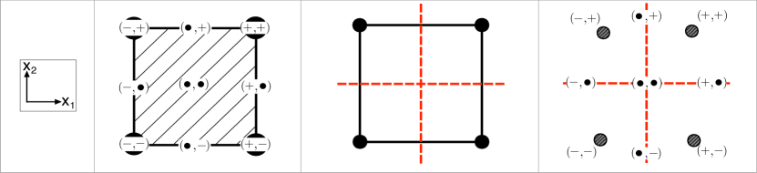
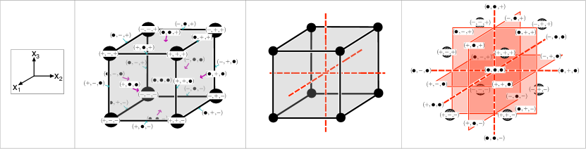
Figure 3: The decomposition and labelings of the cells in a unit hypercube and its dual. The left panels are the original lattice with labels. The middle panels give the lattice (in black) and dual lattice (in red) superimposed on each other. The right panels give the labelings of the dual cells. (Top) Two dimensions. (Bottom) Three dimensions.

III.2 Cochains

We’ll define a cochain $\alpha\in C^{*}({\mathord{{\scalerel*{\Box}{t}}}}_{d},\mathbb{Z}_{2})=C^{0}({\mathord{{\scalerel*{\Box}{t}}}}_{d},\mathbb{Z}_{2})\oplus\cdots\oplus C^{d}({\mathord{{\scalerel*{\Box}{t}}}}_{d},\mathbb{Z}_{2})$ as the set of all functions from $F_{*}({\mathord{{\scalerel*{\Box}{t}}}}_{d})=F_{0}({\mathord{{\scalerel*{\Box}{t}}}}_{d})\sqcup\cdots\sqcup F_{d}({\mathord{{\scalerel*{\Box}{t}}}}_{d})$ to $\mathbb{Z}_{2}=\{0,1\}$. And we’ll say that $\alpha\in C^{p}({\mathord{{\scalerel*{\Box}{t}}}}_{d},\mathbb{Z}_{2})$ for such functions that are only nonzero on $F_{p}({\mathord{{\scalerel*{\Box}{t}}}}_{d})$. For a $p$-cell $P_{(z_{1}\cdots z_{d})}$ denoted as ${\mathord{{\scalerel*{\Box}{t}}}}_{p}$, we define the indicator $p$-cochain $\boldsymbol{{\mathord{{\scalerel*{\Box}{t}}}}}_{p}$ with value $1$ on the cell ${\mathord{{\scalerel*{\Box}{t}}}}_{p}$ and 0 elsewhere.

Now, we define the coboundary operator, $\delta:C^{*}({\mathord{{\scalerel*{\Box}{t}}}}_{d})\to C^{*+1}({\mathord{{\scalerel*{\Box}{t}}}}_{d})$. Just like in simplicial cohomology, the value of $\delta\alpha$ on some $p$-cell $P_{(z_{1}\cdots z_{d})}$ is the sum of the values of $\alpha$ on the boundary $\partial P_{(z_{1}\cdots z_{d})}$, i.e.

$$(\delta\alpha)(z_{1}\cdots z_{d})=\sum_{(\tilde{z}_{1}\cdots\tilde{z}_{d})\in\partial(z_{1}\cdots z_{d})}\alpha(\tilde{z}_{1}\cdots\tilde{z}_{d}).$$ (19)

For example,

$$(\delta\alpha)(\bullet,\bullet,+)=\alpha(\bullet,+,+)+\alpha(\bullet,-,+)+\alpha(+,\bullet,+)+\alpha(-,\bullet,+).$$ (20)

IV $\cup_{m}$ products over $\mathbb{Z}_{2}$

Let’s describe the $\cup_{k}$ products. As described in [T18, T20], the $\cup_{k}$ product on cochains can be thought of as a ‘thickened intersection product’ of cells on the dual cellulation. In particular, $\alpha\cup_{k}\beta$ is dual to $\lim_{\epsilon\to 0}\alpha^{\vee}\cap\beta^{\vee}_{\text{thickened,shifted}}$, where $\alpha^{\vee},\beta^{\vee}$ are the duals of $\alpha,\beta$ respectively, $\beta^{\vee}_{\text{thickened,shifted}}$ is a thickened and shifted version of $\beta$, and $\epsilon$ is some scaling factor for the shifting that indicates we consider this thickened intersection in the limit that the shifting goes to zero.

In [T18, T20], this characterization of the $\cup_{k}$ products was on a triangulation equipped with branching structure, where the branching structure essentially defined the vector fields. In turn, it’s quite subtle to adequetely define the vector fields on a triangulation because triangulations and the associated theory of PL manifolds is subtle . For us in the case of the hypercubic $\mathbb{Z}^{d}$ lattice embedded in $\mathbb{R}^{d}$, things are easier because we can simply choose a constant frame of vector fields to thicken and shift along. Similar to the case of triangulations in [T20], we choose vector fields that form a Vandermonde matrix.

In the main text, we’ll only describe the definitions and some key properties of our $\cup_{m}$ products. Although, we’ll relegate many detailed calculations to the appendices.

IV.1 Definitions and Examples

As described above, our definitions of $\alpha\cup\beta$ and $\alpha\cup_{m}\beta$ were constructed based on what pairs of dual cells intersect each other upon thickening and shifting the dual cells of $\beta$, in the limit as the shifting goes to zero. In particular, the $\cup_{m}$ product will involve thickening $\beta$ along $m$ vector fields. By dimension-counting, if $\alpha$ a $p$-cochain and $\beta$ a $q$-cochain, then $\alpha^{\vee},\beta^{\vee}$ consist of $(d-p)$-cells,$(d-q)$-cells respectively, and so $\alpha^{\vee}\cap\beta^{\vee}_{\text{thickened,shifted}}$ will consist of $(d-p-q+m)$-dimensional submanifolds so we’d want $\alpha\cup_{m}\beta$ to be a $(p+q-m)$-cochain. With this, there’s actually a subtlety that in the limit as the shifting goes to zero; in particular some of the intersecting cells degenerate to lower-dimensional cells in the limit. We do not consider these degenerate cells and instead define the intersection product in terms of those cells that survive as full $(d-p-q+m)$-dimensional cells in the limit. The details of how to derive these formulas is given in Appendix LABEL:app:defininingCupMProducts.

Consider a $d$-cell $(\cdots\bullet_{1}\cdots\bullet_{2}\cdots{\dots}\cdots\bullet_{d}\cdots)$, which consists of $d$ coordinates labeled $\bullet$ and all the rest $\cdots$ are in $\{+,-\}$. Then we’ll have

$$(\alpha\cup_{m}\beta)(\cdots\bullet_{1}\cdots{\dots}\cdots\bullet_{d}\cdots)=\sum_{(\text{cell-1, cell-2})\in\mathrm{Int}_{m}(\cdots\bullet_{1}\cdots\bullet_{2}\cdots{\dots}\cdots\bullet_{d}\cdots)}\alpha(\text{cell-1})\beta(\text{cell-2})$$

which is a a sum over all pairs $(\text{cell-1, cell-2})$ in the set $\mathrm{Int}_{m}(\cdots\bullet_{1}\cdots\bullet_{2}\cdots{\dots}\cdots\bullet_{d}\cdots)$ of pairs of cells whose duals survive as full-dimensional as described above.

Soon, we’ll write out the explicit pairs that appear in $\mathrm{Int}(\bullet_{1}{\dots}\bullet_{d})$ when all coordinates are ‘$\bullet$’. This is actually all the information we need. In particular, all surviving pairs $(\text{cell-1, cell-2})\in\mathrm{Int}_{m}(\cdots\bullet_{1}\cdots\bullet_{2}\cdots{\dots}\cdots\bullet_{d}\cdots)$ must have all of the $\cdots=\pm$ coordinates of $(\cdots\bullet_{1}\cdots\bullet_{2}\cdots{\dots}\cdots\bullet_{d}\cdots)$ shared by both of ‘cell-1’ and ‘cell-2’. And, the $\bullet_{1}\cdots\bullet_{d}$ coordinates that are possibly replaced by $\pm$ in cell-1, cell-2 will occur in the same way as they would’ve been in $\mathrm{Int}_{m}(\bullet_{1}\cdots\bullet_{d})$. For example, we’d have:

$$(\alpha\cup_{m}\beta)(\bullet,-,\bullet,\bullet,+)=\sum_{((z_{1},z_{2},z_{3}),(z^{\prime}_{1},z^{\prime}_{2},z^{\prime}_{3}))\in\mathrm{Int}_{m}(\bullet,\bullet,\bullet)}\alpha(z_{1},-,z_{2},z_{3},+)\beta(z^{\prime}_{1},-,z^{\prime}_{2},z^{\prime}_{3},+)$$

Our descriptions of $\mathrm{Int}_{m}(\bullet_{1}\cdots\bullet_{d})$ will involve pairs of cells of dimensions $p,q$ with $p+q-m=d$. As such, these pairs correspond to the full product $C^{*_{1}}({\mathord{{\scalerel*{\Box}{t}}}}_{d})\times C^{*_{2}}({\mathord{{\scalerel*{\Box}{t}}}}_{d})\to C^{*_{1}+*_{2}-m}({\mathord{{\scalerel*{\Box}{t}}}}_{d})$ on the graded cochain ring on a single ${\mathord{{\scalerel*{\Box}{t}}}}_{d}$. To get a formula for a specific product $C^{p}({\mathord{{\scalerel*{\Box}{t}}}}_{d})\times C^{q}({\mathord{{\scalerel*{\Box}{t}}}}_{d})\to C^{p+q-m}({\mathord{{\scalerel*{\Box}{t}}}}_{d})$, one can restrict to pairs in $\mathrm{Int}_{m}(\bullet_{1}\cdots\bullet_{d})$ where cell-1,cell-2 have dimensions $p,q$ respectively.

Now we describe $\mathrm{Int}_{m}(\bullet_{1}\cdots\bullet_{d})$. In general, this set will consist of pairs $((z_{1}\cdots z_{d}),(z^{\prime}_{1},\cdots,z^{\prime}_{d}))$ such that for $m$ coordinates $1\leq i_{1}<\cdots<i_{m}\leq d$ both the $z,z^{\prime}$ entries are $\bullet$; i.e. $z_{i_{1}}=z^{\prime}_{i_{1}}=\cdots=z_{i_{m}}=z^{\prime}_{i_{m}}=\bullet$. Given these $i_{1}<\cdots<i_{m}$, we’ll have that $(z_{j},z^{\prime}_{j})$ for $j\not\in\{i_{1},\cdots,i_{m}\}$ depend on the position of $j$ relative to the $i_{1}<\cdots<i_{m}$. First, defining $i_{0}:=0$ and $i_{d+1}=d+1$, we have that there is a unique $\ell(j)\in\{0,\cdots,d\}$ for which $i_{\ell(j)}<j<i_{\ell(j)+1}$. Given this, we’ll have that $(z_{j},z^{\prime}_{j})\in\{((-1)^{\ell(j)}+,\bullet),(\bullet,(-1)^{\ell(j)}-)\}$ where we mean “$(-1)\cdot+=-$” and “$(-1)\cdot-=+$”. In short, the definition is:

Definition 1.

$$\begin{split}\mathrm{Int}_{m}(\bullet_{1}\cdots\bullet_{d})=\bigcup\limits_{\{1\leq i_{1}<\cdots i_{m}\leq d\}}\bigg{\{}((z_{1}\cdots z_{d}),(z^{\prime}_{1}\cdots z^{\prime}_{d}))\bigg{|}&z_{i_{1}}=z^{\prime}_{i_{1}}=\cdots=z_{i_{m}}=z^{\prime}_{i_{m}}=\bullet,\text{ and }\\ &\text{ each }(z_{j},z^{\prime}_{j})\in\{((-1)^{\ell(j)}+,\bullet),(\bullet,(-1)^{\ell(j)}-)\}\bigg{\}},\end{split}$$ (21)

and

$$(\alpha\cup_{m}\beta)(\bullet_{1}\cdots\bullet_{d})=\sum_{((z_{1},\cdots,z_{d}),(z^{\prime}_{1},\cdots,z^{\prime}_{d}))\in\mathrm{Int}_{m}(\bullet_{1}\cdots\bullet_{d})}\alpha(z_{1},\cdots,z_{d})\beta(z^{\prime}_{1},\cdots,z^{\prime}_{d})$$ (22)

In general, $(\alpha\cup_{0}\beta)(z_{1}\cdots z_{d})$ will have $2^{k}$ terms, where $k$ is the number of elements in the set $S\equiv\{i|z_{i}=\bullet\}$. For each $i\in S$, there are two choices for the arguments in $\alpha$ and $\beta$: $\alpha(\cdots,\bullet_{i},\cdots)\beta(\cdots,-_{i},\cdots)$ or $\alpha(\cdots,+_{i},\cdots)\beta(\cdots,\bullet_{i},\cdots)$ Similarly, $(\alpha\cup_{m}\beta)(\bullet_{1}\cdots\bullet_{d})$ will have ${d\choose m}\cdot 2^{d-m}$ terms which correspond to those choices $\{i_{1}<\cdots<i_{m}\}$ and the two choices of $(z_{j},z^{\prime}_{j})$ for $j\not\in\{i_{1}\cdots i_{m}\}$. Although, only some of these terms appear in the restriction to each $C^{p}\times C^{q}\to C^{p+q-m}$.

Now we spell out a few examples, starting with $\cup_{0}$. First in $d=3$, we’ll have that:

$$\begin{split}(\alpha\cup_{0}\beta)(\bullet,\bullet,\bullet)=&\alpha(\bullet,\bullet,\bullet)\beta(-,-,-)+\alpha(\bullet,\bullet,+)\beta(-,-,\bullet)+\alpha(\bullet,+,\bullet)\beta(-,\bullet,-)+\alpha(+,\bullet,\bullet)\beta(\bullet,-,-)\\ +&\alpha(\bullet,+,+)\beta(-,\bullet,\bullet)+\alpha(+,\bullet,+)\beta(\bullet,-,\bullet)+\alpha(+,+,\bullet)\beta(\bullet,\bullet,-)+\alpha(+,+,+)\beta(\bullet,\bullet,\bullet)\\ \end{split}$$

Note that every term $\alpha(z^{\prime}_{1},z^{\prime}_{2},z^{\prime}_{3})\beta(z^{\prime\prime}_{1},z^{\prime\prime}_{2},z^{\prime\prime}_{3})$ above has exactly one of $z^{\prime}_{k}$ or $z^{\prime\prime}_{k}$ equalling $\bullet$ for $k=1,2,3$. And, if $z^{\prime}_{k}=\bullet$ then $z^{\prime\prime}_{k}=-$, and if $z^{\prime\prime}_{k}=\bullet$ then $z^{\prime}_{k}=+$. Another example is:

$$(\alpha\cup_{0}\beta)(\bullet,\bullet,\pm)=\alpha(\bullet,\bullet,\pm)\beta(-,-,\pm)+\alpha(\bullet,+,\pm)\beta(-,\bullet,\pm)+\alpha(+,\bullet,\pm)\beta(\bullet,-,\pm)+\alpha(+,+,\pm)\beta(\bullet,\bullet,\pm)$$

where $\pm$ refers to either choice of $+$ or $-$. Note for any term $\alpha(z^{\prime}_{1},z^{\prime}_{2},z^{\prime}_{3})\beta(z^{\prime\prime}_{1},z^{\prime\prime}_{2},z^{\prime\prime}_{3})$, we have that $z^{\prime}_{3}=z^{\prime\prime}_{3}=\pm$, matching with the third term of the argument of $(\alpha\cup_{0}\beta)(z_{1},z_{2},z_{3})$. And since $z_{1}=z_{2}=\bullet$, the same pattern as the previous example works. That exactly one of $z^{\prime}_{k}$ or $z^{\prime\prime}_{k}$ is $\bullet$ for $k=1,2$. And if $z^{\prime}_{k}=\bullet$ then $z^{\prime\prime}_{k}=-$, and if $z^{\prime\prime}_{k}=\bullet$ then $z^{\prime}_{k}=-$.

As an example of the $\cup_{1}$ product, in $d=3$, we’ll have:

$$\begin{split}(\alpha\cup_{1}\beta)(\bullet,\bullet,\bullet)&=\alpha(\bullet,\bullet,\bullet)\beta(-,-,\bullet)+\alpha(\bullet,+,\bullet)\beta(-,\bullet,\bullet)+\alpha(+,\bullet,\bullet)\beta(\bullet,-,\bullet)+\alpha(+,+,\bullet)\beta(\bullet,\bullet,\bullet)\\ &+\alpha(\bullet,\bullet,\bullet)\beta(-,\bullet,+)+\alpha(\bullet,\bullet,-)\beta(-,\bullet,\bullet)+\alpha(+,\bullet,\bullet)\beta(\bullet,\bullet,+)+\alpha(+,\bullet,-)\beta(\bullet,\bullet,\bullet)\\ &+\alpha(\bullet,\bullet,\bullet)\beta(\bullet,+,+)+\alpha(\bullet,\bullet,-)\beta(\bullet,+,\bullet)+\alpha(\bullet,-,\bullet)\beta(\bullet,\bullet,+)+\alpha(\bullet,-,-)\beta(\bullet,\bullet,\bullet)\end{split}$$

See Fig. 4 for the geometric depiction of some of these examples.

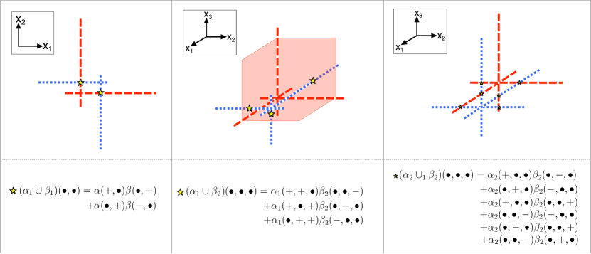
Figure 4: Geometric depictions of (Left) the $\cup_{0}$ product between 1-cochains in two dimensions, (Middle) the $\cup_{0}$ product between a 2-cochain and a 1-cochain in three dimensions, and (Right) the $\cup_{1}$ product of 2-cochains in three dimensions.

IV.2 Diagrammatics

Now, we’ll introduce a convenient way to diagrammatically represent the $\cup_{m}$ products. These diagrammatics will be helpful in establishing the identity $\delta(\alpha\cup_{m}\beta)=\delta\alpha\cup_{m}\beta+\alpha\cup_{m}\delta\beta+\alpha\cup_{m-1}\beta+\beta\cup_{m-1}\alpha$.

First, we’ll only need to care about the case of $(\alpha\cup_{0}\beta)(\bullet\cdots\bullet)$ where all the arguments are all $\bullet$. This is because if any other arguments are $+$ or $-$, then the corresponding arguments for $\alpha$ and $\beta$ are fixed and equal to the $+$ or $-$. The diagrammatics are summarized in Fig. 5.

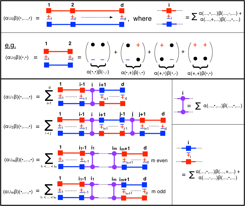
Figure 5: Diagrammatic representations of: (top) $\alpha\cup_{0}\beta$ (Bottom) $\alpha\cup_{m}\beta$

In the Appendix LABEL:app:proofOfHigherCupId, we show how to think about the diagrammatics with respect to the coboundary operators $\delta$ and show the fundamental cup and higher cup product identities:

Proposition 1.

$\delta(\alpha\cup\beta)=\delta\alpha\cup\beta+\alpha\cup\delta\beta$

Proposition 2.

$\delta(\alpha\cup_{m}\beta)=\delta\alpha\cup_{m}\beta+\alpha\cup_{m}\delta\beta+\alpha\cup_{m-1}\beta+\beta\cup_{m-1}\alpha$.

V Cochain operations over $\mathbb{Z}$

Here, we describe how to extend the definition of the boundary operator $\delta$ and the $\cup_{0}$ product to cochains over $\mathbb{Z}$.

V.1 $\delta$ over $\mathbb{Z}$

First, we define the coboundary operator $\delta$ acting on a $(d-1)$-cochain $\alpha$ as

$$(\delta\alpha)(\bullet_{1},\cdots,\bullet_{d})=\sum_{\begin{subarray}{c}\ell=1,\\ \pm\in\{+,-\}\end{subarray}}^{d}\mp(-1)^{\ell}\alpha(\bullet,\cdots\underbrace{,\pm,}_{\begin{subarray}{c}\ell^{\text{th}}\\ \text{coord.}\end{subarray}}\cdots,\bullet)$$ (23)

where $\mp=-\pm$. In general for an $n$-cochain, $\delta\alpha$ can be defined similarly to the $\mathbb{Z}_{2}$ on $(\delta\alpha)(\cdots,\bullet_{i_{1}},\cdots,\bullet_{i_{2}},\cdots,\bullet_{i_{n}},\cdots)$ where there are $n$ coordinates $\{\bullet_{i_{k}}\}_{k=1}^{n}$ and $(d-n)$ coordinates $\pm$. Then we can define $\delta$ by keeping all the $\pm$ coordinates fixed and only altering the $\bullet$ coordinates one at a time

$$(\delta\alpha)(\cdots,\bullet_{i_{1}},\cdots,\bullet_{i_{2}},\cdots,\bullet_{i_{n}},\cdots)=\sum_{\begin{subarray}{c}\ell=1,\\ \pm\in\{+,-\}\end{subarray}}^{n}\mp(-1)^{\ell}\alpha(\cdots\underbrace{,\pm,}_{\begin{subarray}{c}{i_{\ell}}^{\text{th}}\\ \text{coord.}\end{subarray}}\cdots)$$ (24)

and the sign $\mp(-1)^{\ell}$ in front of each term only depends on $\pm$ and the coordinate $\ell$ that defines the position of $\bullet_{i_{\ell}}$ with respect to all the other $\bullet$ positions. Note that the equation

$$\delta\delta\alpha=0$$ (25)

will follow from essentially same reasoning as in the simplicial case.

V.2 $\cup_{0}:=\cup$ over $\mathbb{Z}$

Now we’ll define a cup-product operation $\cup_{0}:=\cup$ over $\mathbb{Z}$. It satisfies the following cochain-level Leibniz-rule, with respect to the $n$-cochain $\alpha^{n}$ and $m$-cochain $\beta^{m}$

$$\delta(\alpha^{n}\cup\beta^{m})=(\delta\alpha^{n})\cup\beta^{m}+(-1)^{n}\alpha^{n}\cup(\delta\beta^{m}).$$

Now, we restrict our attention to case where $n+m=d$ to define the $\cup$ product. The other cases where $n+m<d$ can again be specified by keeping the signs fixed away from $(n+m)$ $\bullet$-coordinates in $(\alpha\cup\beta)(\cdots,\bullet_{i_{1}},\cdots,\bullet_{i_{2}},\cdots,\bullet_{i_{n}},\cdots)$ as in all previous discussion. Now define

$$(\alpha^{n}\cup\beta^{d-n})(\bullet_{1},\cdots,\bullet_{d})=\sum_{\begin{subarray}{c}(z_{1}\cdots z_{d}),(z^{\prime}_{1}\cdots z^{\prime}_{d})\\ z_{i}=+\text{ and }z^{\prime}_{i}=\bullet\text{, OR}\\ z_{i}=\bullet\text{ and }z^{\prime}_{i}=-\end{subarray}}(-1)^{s}\alpha(z_{1}\cdots z_{d})\beta(z^{\prime}_{1}\cdots z^{\prime}_{d})$$ (26)

where the sign $(-1)^{s}$ will be defined in a moment. First note that the (mod 2) reduction of this exactly agrees with our formulas and diagrammatics over $\mathbb{Z}_{2}$. To define $(-1)^{s}$ on the term associated to $(z_{1}\cdots z_{d}),(z^{\prime}_{1}\cdots z^{\prime}_{d})$, we first define $a_{1}\cdots a_{d-n}$ as the $z_{i}$ that are labeled $+$ and define $b_{1}\cdots b_{n}$ as the $z^{\prime}_{i}$ that are labeled $-$. Then, we can define $(-1)^{s}$ as

$$(-1)^{s}=\underbrace{(-1)^{d-n}}_{\begin{subarray}{c}-1\text{ for each}\\ +\text{ label}\end{subarray}}\text{sgn}\begin{pmatrix}1&\cdots&\cdots&\cdots&\cdots&d\\ b_{1}&\to&b_{n}&a_{1}&\to&a_{d-n}\end{pmatrix}\cdot(-1)^{m}$$ (27)

with respect to the sign of the permutation taking $(1\to d)$ to $(b_{1}\cdots b_{n};a_{1}\cdots a_{d-n})$.

We note that this sign is closely related to a signed intersection between the cell dual to $\beta$ and the cells dual to $\alpha$. In particular, the dual cells corresponding to $(z_{1}\cdots z_{d}),(z^{\prime}_{1}\cdots z^{\prime}_{d})$ will extend out in the $b_{1},\dots,b_{n}$ directions for $\beta$’s dual and in the $a_{1},\dots,a_{d-n}$ directions for $\alpha$. As such, the above sign can roughly be thought of as representing a “$\beta^{\text{dual}}\cap\alpha^{\text{dual}}$” with signs in analog to how the $\cup$ product in cohomology is dual to signed intersections of the dual submanifolds.

We state the Leibniz rule.

Proposition 3.

$\delta(\alpha^{n}\cup\beta^{m})=(\delta\alpha^{n})\cup\beta^{m}+(-1)^{n}\alpha^{n}\cup(\delta\beta^{m})$ where $\alpha^{n}$ and $\beta^{m}$ are $n$- and $m$-cochains respectively.

The proof is given in Appendix LABEL:app:proofOfCupM_OverZ together with an analogous one for the $\cup_{k}$ products, defined below.

V.3 $\cup_{k}$ over $\mathbb{Z}$

In general, a similar pattern works for the higher cup operations over $\mathbb{Z}$ which we’ll call the $\cup_{k}$ products because of the minor differences in the formulas as compared to Steenrod’s formulas. We give the definition for $\alpha^{n+k}\cup_{k}\beta^{d-n}$ analogous to our $\mathbb{Z}_{2}$ definitions

$$(\alpha^{n+k}\cup_{k}\beta^{d-n})(\bullet_{1},\cdots,\bullet_{d}):=\sum_{1=:i_{0}\leq i_{1}<\cdots<i_{k}\leq i_{k+1}:=d}\sum_{\begin{subarray}{c}(z_{1}\cdots z_{d}),(z^{\prime}_{1}\cdots z^{\prime}_{d})\\ \text{each }z_{i_{1}}=z^{\prime}_{i_{1}}=\cdots=z_{i_{k}}=z^{\prime}_{i_{k}}=\bullet\\ z_{j}=(-1)^{\ell(j)}+\text{ and }z^{\prime}_{j}=\bullet\text{, OR}\\ z_{j}=\bullet\text{ and }z^{\prime}_{j}=(-1)^{\ell(j)}-\\ \text{where }i_{\ell(j)}<j<i_{\ell(j)+1}\end{subarray}}(-1)^{s}\alpha(z_{1}\cdots z_{d})\beta(z^{\prime}_{1}\cdots z^{\prime}_{d})$$ (28)

Here the sign $(-1)^{s}$ on each depends on $(i_{1}\cdots i_{k})$ and $(z_{1}\cdots z_{d}),(z^{\prime}_{1}\cdots z^{\prime}_{d})$. Again we can define $b_{1}<\cdots<b_{n}$ as the coordinates in $z^{\prime}_{1}\cdots z^{\prime}_{d}$ that are labeled by $\pm$. And define $a_{1}\cdots a_{d-n-k}$ as the coordinates in $z_{1}\cdots z_{d}$ labeled as $\pm$. Then we’ll set

$$(-1)^{s}=(-1)^{\text{\# of total + signs}}\text{sgn}\begin{pmatrix}1&\cdots&\cdots&\cdots&\cdots&\cdots&\cdots&\cdots&d\\ i_{1}&\to&i_{k}&b_{1}&\to&b_{n}&a_{1}&\to&a_{d-n-k}\end{pmatrix}\cdot(-1)^{k+(d-n)+(n-k-1)k}$$ (29)

where the “# of total + signs” is the total number of $+$ coordinates among both $(z_{1}\cdots z_{d}),(z^{\prime}_{1}\cdots z^{\prime}_{d})$. This can also be interpreted as a signed intersection of $\beta^{\vee}_{\text{thickened,shifted}}\cap\alpha^{\vee}$. Then we’ll have the cochain-level identity:

Proposition 4.

Let $\alpha$ be an $(n-1+k)$-cochain and $\beta$ be an $(d-n)$-cochain. Then

$$\begin{split}\delta(\alpha^{n-1+k}\cup_{k}\beta^{d-n})=\delta\alpha\cup_{k}\beta+(-1)^{n-1+k}\alpha\cup_{k}\delta\beta+(-1)^{d-1}\alpha\cup_{k-1}\beta+(-1)^{(n-1+k)(d-n)-1+k+d}\beta\cup_{k-1}\alpha.\end{split}$$ (30)

Note that defining $p=n-1+k$ and $q=d-n$, the above product is exactly the recursion relation $\delta(\alpha^{p}\cup_{k}\beta^{q})=\delta\alpha\cup_{k}\beta+(-1)^{p}\alpha\cup_{k}\delta\beta+(-1)^{p+q-k}\alpha\cup_{k-1}\beta+(-1)^{pq+p+q}\beta\cup_{k-1}\alpha$ of Steenrod [S47]. See Appendix LABEL:app:proofOfCupM_OverZ for a proof.

VI Fermions: Exact Bosonziation and Grassmann Integral

We will now apply the $\mathbb{Z}_{2}$ higher-cup formalism to express lattice models of fermions on a hypercubic lattice. We first ‘bosonize’ fermionic operator algebras that are defined on a hypercubic lattice, generalizing the constructions of [chen2020BosonArbDimensions]. The paper [chen2020BosonArbDimensions] considered a triangulated $d$-manifold where there was one copy of fermion operators $\gamma_{\Delta_{d}},\gamma^{\prime}_{\Delta_{d}}$ for each $d$-simplex. It was shown that one can express all even-fermion-parity operators in that algebra in terms of an algebra of bosonic Pauli operators $X_{\Delta_{d-1}},Z_{\Delta_{d-1}}$ associated to each $(d-1)$-simplex of the triangulation in the presence of an additional gauge constraint. The bosonization map used the $\cup_{m}$ products on a triangulation. We’ll show here that essentially the same map holds on a hypercubic lattice if one considers the hypercubic $\cup_{m}$ products defined here.

After this, we will also extend the ‘Gu-Wen Grassmann Integral’ [guWen2014Supercohomology] $\sigma(\alpha)$ to hypercubic lattices, which can be used in space-time path-integral constructions of fermionic phases of matter. We review two definitions of $\sigma(\alpha)$, via winding numbers on winding numbers on curves and via Grassmann variables.

In Sec. LABEL:sec:fermionicToricCode, we will define a ‘fermionic toric code’ model in arbitary dimensions on the hypercubic lattice, similar to [chen2020BosonArbDimensions]. This will use the exact bosonization map and also have a close relation to the Grassmann integral.

VI.1 Exact Bosonization

Now, let’s spell out the exact bosonization map on the hypercubic lattice $\mathbb{Z}^{d}$, which corresponds to maps between $(d+1)$-dimensional Hamiltonians. We’ll be given a system of fermions generated by $\gamma_{{\mathord{{\scalerel*{\Box}{t}}}}_{d}},\gamma^{\prime}_{{\mathord{{\scalerel*{\Box}{t}}}}_{d}}$ living at the centers of the $d$-dimensional hypercubes (or equivalently on the vertices of the dual lattice). And on the bosonic side, we’ll have Pauli matrices $X_{{\mathord{{\scalerel*{\Box}{t}}}}_{d-1}},Z_{{\mathord{{\scalerel*{\Box}{t}}}}_{d-1}}$ living on $(d-1)$-simplices. The duality is:

$$W_{{\mathord{{\scalerel*{\Box}{t}}}}_{d}}:=\prod_{{\mathord{{\scalerel*{\Box}{t}}}}_{d-1}\subset{\mathord{{\scalerel*{\Box}{t}}}}_{d}}Z_{{\mathord{{\scalerel*{\Box}{t}}}}_{d-1}} \longleftrightarrow P_{{\mathord{{\scalerel*{\Box}{t}}}}_{d}}:=-i\gamma_{{\mathord{{\scalerel*{\Box}{t}}}}_{d}}\gamma^{\prime}_{{\mathord{{\scalerel*{\Box}{t}}}}_{d}}$$ (31)

$${U}_{{\mathord{{\scalerel*{\Box}{t}}}}_{d-1}}:=X_{{\mathord{{\scalerel*{\Box}{t}}}}_{d-1}}\left(\prod_{{\mathord{{\scalerel*{\Box}{t}}}}^{\prime}_{d-1}}Z_{{\mathord{{\scalerel*{\Box}{t}}}}_{d-1}}^{\int{\boldsymbol{{\mathord{{\scalerel*{\Box}{t}}}}}}^{\prime}_{d-1}\cup_{d-2}{\boldsymbol{{\mathord{{\scalerel*{\Box}{t}}}}}}_{d-1}}\right) \longleftrightarrow S_{{\mathord{{\scalerel*{\Box}{t}}}}_{d-1}}:=i\gamma_{L({\mathord{{\scalerel*{\Box}{t}}}}_{d-1})}\gamma^{\prime}_{R({\mathord{{\scalerel*{\Box}{t}}}}_{d-1})}$$ (32)

$$G_{{\mathord{{\scalerel*{\Box}{t}}}}_{d-2}}:=\underbrace{\prod_{{\mathord{{\scalerel*{\Box}{t}}}}_{d-1}\supset{\mathord{{\scalerel*{\Box}{t}}}}_{d-2}}X_{{\mathord{{\scalerel*{\Box}{t}}}}_{d-1}}\left(\prod_{{\mathord{{\scalerel*{\Box}{t}}}}^{\prime}_{d-1}}Z_{{\mathord{{\scalerel*{\Box}{t}}}}^{\prime}_{d-1}}^{\int\delta\boldsymbol{{\mathord{{\scalerel*{\Box}{t}}}}}_{d-2}\cup_{d-2}\boldsymbol{{\mathord{{\scalerel*{\Box}{t}}}}}^{\prime}_{d-1}}\right)}_{\text{Set equal to }1\text{ as gauge constraint}}=1 \longleftrightarrow\underbrace{S_{\delta\boldsymbol{{\mathord{{\scalerel*{\Box}{t}}}}}_{d-2}}\prod_{{\mathord{{\scalerel*{\Box}{t}}}}_{d}}P_{{\mathord{{\scalerel*{\Box}{t}}}}_{d}}^{\int\boldsymbol{{\mathord{{\scalerel*{\Box}{t}}}}}_{d}\cup_{d-1}\delta\boldsymbol{{\mathord{{\scalerel*{\Box}{t}}}}}_{d-2}}}_{\text{Equals }1\text{ as an identity}}=1.$$ (33)

The first two Eqs. (31,32) above are identities between the operator algebras, with the $P_{{\mathord{{\scalerel*{\Box}{t}}}}_{d}}$ representing fermion parity inside ${\mathord{{\scalerel*{\Box}{t}}}}_{d}$ and $S_{{\mathord{{\scalerel*{\Box}{t}}}}_{d-1}}$ being a hopping operator across ${\mathord{{\scalerel*{\Box}{t}}}}_{d-1}$. The last Eq. (33) gives the required gauge constraint on the bosonic LHS while the fermionic RHS is an identity that always holds (that we’ll show soon). The rest of this section will demonstrate this bosonization, although we defer many details to [chen2020BosonArbDimensions] because the proofs are similar. We start by explaining some notation above, in particular what we mean by $L({\mathord{{\scalerel*{\Box}{t}}}}_{d-1}),R({\mathord{{\scalerel*{\Box}{t}}}}_{d-1})$ and $S_{\lambda}$ for a general cochain $\lambda$.

First, given a $(d-1)$-hypercube ${\mathord{{\scalerel*{\Box}{t}}}}_{d-1}$, there are two $d$-hypercubes $L({\mathord{{\scalerel*{\Box}{t}}}}_{d-1}),R({\mathord{{\scalerel*{\Box}{t}}}}_{d-1})$ that it’s adjacent to. Supposing ${\mathord{{\scalerel*{\Box}{t}}}}_{d-1}$ is in the $\{1\cdots\hat{\imath}\cdots d\}$ hyperplane, the two adjacent ${\mathord{{\scalerel*{\Box}{t}}}}_{d}$’s will be in the two $\pm x_{\hat{\imath}}$ directions relative to ${\mathord{{\scalerel*{\Box}{t}}}}_{d-1}$, which we’ll call ${{}^{+}}({\mathord{{\scalerel*{\Box}{t}}}}_{d-1}),{{}^{-}}({\mathord{{\scalerel*{\Box}{t}}}}_{d-1})$ respectively. We’ll define

$$\big{(}L({\mathord{{\scalerel*{\Box}{t}}}}_{d-1}),R({\mathord{{\scalerel*{\Box}{t}}}}_{d-1})\big{)}=\begin{cases}\big{(}{{}^{-}}({\mathord{{\scalerel*{\Box}{t}}}}_{d-1}),{{}^{+}}({\mathord{{\scalerel*{\Box}{t}}}}_{d-1})\big{)}\,\text{ if }i+d=1\text{ (mod 2)}\\ \big{(}{{}^{+}}({\mathord{{\scalerel*{\Box}{t}}}}_{d-1}),{{}^{-}}({\mathord{{\scalerel*{\Box}{t}}}}_{d-1})\big{)}\,\text{ if }i+d=0\text{ (mod 2)}\\ \end{cases}$$ (35)

which is depicted in Fig. 6.

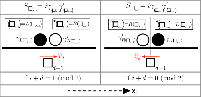
Figure 6: Definitions of $L({\mathord{{\scalerel*{\Box}{t}}}}_{d-1})$ and $R({\mathord{{\scalerel*{\Box}{t}}}}_{d-1})$ depending on $i+d\text{ (mod 2)}$. The $+x_{i}$ direction is to the right and determine the definitions of ${{}^{\pm}}({\mathord{{\scalerel*{\Box}{t}}}}_{d-1})$. The $\gamma,\gamma^{\prime}$ are given be the solid-black,open-white circles respectively. A useful reference is the red arrow labeled $\widehat{v}_{d}$ is the direction of the vector field $\widehat{v}_{d}$ that’s parallel to the dual 1-skeleton, as defined in the Appendix LABEL:app:framingsOfCurvesAndWindings; it is used to define the left/right sides of ${\mathord{{\scalerel*{\Box}{t}}}}_{d-1}$.

Now, to define $S_{\lambda}$ for a general $(d-1)$-cochain $\lambda$, we will need the following equality of the commutation relations of the $S_{{\mathord{{\scalerel*{\Box}{t}}}}_{d-1}}$ and ${U}_{{\mathord{{\scalerel*{\Box}{t}}}}_{d-1}}$ which match:

Lemma 5.

$$S_{{\mathord{{\scalerel*{\Box}{t}}}}_{d-1}}S_{{\mathord{{\scalerel*{\Box}{t}}}}^{\prime}_{d-1}}=S_{{\mathord{{\scalerel*{\Box}{t}}}}^{\prime}_{d-1}}S_{{\mathord{{\scalerel*{\Box}{t}}}}_{d-1}}(-1)^{\int\boldsymbol{{\mathord{{\scalerel*{\Box}{t}}}}}_{d-1}\cup_{d-2}\boldsymbol{{\mathord{{\scalerel*{\Box}{t}}}}}^{\prime}_{d-1}+\boldsymbol{{\mathord{{\scalerel*{\Box}{t}}}}}^{\prime}_{d-1}\cup_{d-2}\boldsymbol{{\mathord{{\scalerel*{\Box}{t}}}}}_{d-1}}$$ (36)

and

$${U}_{{\mathord{{\scalerel*{\Box}{t}}}}_{d-1}}{U}_{{\mathord{{\scalerel*{\Box}{t}}}}^{\prime}_{d-1}}={U}_{{\mathord{{\scalerel*{\Box}{t}}}}^{\prime}_{d-1}}{U}_{{\mathord{{\scalerel*{\Box}{t}}}}_{d-1}}(-1)^{\int\boldsymbol{{\mathord{{\scalerel*{\Box}{t}}}}}_{d-1}\cup_{d-2}\boldsymbol{{\mathord{{\scalerel*{\Box}{t}}}}}^{\prime}_{d-1}+\boldsymbol{{\mathord{{\scalerel*{\Box}{t}}}}}^{\prime}_{d-1}\cup_{d-2}\boldsymbol{{\mathord{{\scalerel*{\Box}{t}}}}}_{d-1}}$$ (37)

Note that the second equality for ${U}$ follows immediately from their definition, so we only need to check the first equality for the $S$. We save the proof to the end of this subsection.

Assuming this lemma, we can make a definition of $S_{\lambda}$ for general $(d-1)$-cochains $\lambda$. Say that $\lambda=\lambda_{1}+\cdots+\lambda_{N}$ where each $\lambda_{i}$ is an indicator cochain on a single ${\mathord{{\scalerel*{\Box}{t}}}}_{d-1}$. Then, we’ll define

$$S_{\lambda}:=(-1)^{\sum_{1\leq i<j\leq N}\int\lambda_{i}\cup_{d-2}\lambda_{j}}\prod_{i=1}^{N}S_{\lambda_{i}}.$$ (38)

where the products of the $\{S_{\lambda_{i}}\}$ are in the order $1\to\cdots\to N$. The commutation relations of the $S$ as in Lemma 5 show that this definition is independent of the order of the $\lambda_{i}$, thus is well-defined.

Now, we discuss the fermionic identity on the RHS of Eq. (33), given by the following lemma.

Lemma 6.

For all ${\mathord{{\scalerel*{\Box}{t}}}}_{d-2}$, we have

$$S_{\delta\boldsymbol{{\mathord{{\scalerel*{\Box}{t}}}}}_{d-2}}=\prod_{{\mathord{{\scalerel*{\Box}{t}}}}_{d}}P_{{\mathord{{\scalerel*{\Box}{t}}}}_{d}}^{\int\boldsymbol{{\mathord{{\scalerel*{\Box}{t}}}}}_{d}\cup_{d-1}\delta\boldsymbol{{\mathord{{\scalerel*{\Box}{t}}}}}_{d-2}}$$ (39)

Again, we save the proof to the end of this subsection.

These are the main calculations needed to verify the exact bosonization. The rest of the arguments verifying the equalities of operators algebras carry over mutatis mutandi from [chen2020BosonArbDimensions].

VI.1.1 Proofs of Lemmas 5,6

Now we discuss the proofs of Lemmas 5,6. Before starting the proofs, it’s helpful to state a formula for the $\cup_{d-2}$ product of two $(d-1)$-cochains. We’ll use the notation for each choice of $\{i,\pm\}$

$$\hat{\imath}_{\pm}:=P_{(\bullet,\cdots,\bullet,\underbrace{\pm}_{\text{position `i'}},\bullet,\cdots,\bullet)}$$ (40)

to denote both the $(d-1)$-hypercube above and also as an argument for cochains. The following formula holds

$$(\alpha\cup_{d-2}\beta)({\mathord{{\scalerel*{\Box}{t}}}}_{d})=\sum_{1\leq i<j\leq d}(\alpha(\hat{\imath}_{(-1)^{i+1}})\beta(\hat{\jmath}_{(-1)^{j+1}})+\beta(\hat{\imath}_{(-1)^{i}})\alpha(\hat{\jmath}_{(-1)^{j}}))$$ (41)

where $\hat{\imath}_{\pm 1},\hat{\jmath}_{\pm 1}$ refer to the indices on the cells $\hat{\imath}_{\pm},\hat{\jmath}_{\pm}$. This can be shown using the $\cup_{m}$ formulas presented previously. For example, in $d=4$ we have

$$\begin{split}(\alpha\cup_{d-2}\beta)({\mathord{{\scalerel*{\Box}{t}}}}_{d})=&\alpha(\hat{1}_{+})\beta(\hat{2}_{-})+\alpha(\hat{1}_{+})\beta(\hat{3}_{+})+\alpha(\hat{1}_{+})\beta(\hat{4}_{-})+\alpha(\hat{2}_{-})\beta(\hat{3}_{+})+\alpha(\hat{2}_{-})\beta(\hat{4}_{-})+\alpha(\hat{3}_{+})\beta(\hat{4}_{-})\\ +&\beta(\hat{1}_{-})\alpha(\hat{2}_{+})+\beta(\hat{1}_{-})\alpha(\hat{3}_{-})+\beta(\hat{1}_{-})\alpha(\hat{4}_{+})+\beta(\hat{2}_{+})\alpha(\hat{3}_{-})+\beta(\hat{2}_{+})\alpha(\hat{4}_{+})+\beta(\hat{3}_{-})\alpha(\hat{4}_{+})\end{split}$$

and for all $d<4$, the expression is simply the restriction to terms not involving $\hat{\imath}$ with $i>d$. The analogous pattern holds for all $d$.

Now we prove the Lemma 5.

Proof of Lemma 5.

Write $S_{{\mathord{{\scalerel*{\Box}{t}}}}_{d-1}}=i\gamma_{A}\gamma^{\prime}_{B}$ and $S_{{\mathord{{\scalerel*{\Box}{t}}}}^{\prime}_{d-1}}=i\gamma_{C}\gamma^{\prime}_{D}$ where $A=L({\mathord{{\scalerel*{\Box}{t}}}}_{d-1}),B=R({\mathord{{\scalerel*{\Box}{t}}}}_{d-1})$ and $C=L({\mathord{{\scalerel*{\Box}{t}}}}^{\prime}_{d-1}),D=R({\mathord{{\scalerel*{\Box}{t}}}}^{\prime}_{d-1})$ are the $d$-hypercubes that $S_{{\mathord{{\scalerel*{\Box}{t}}}}_{d-1}}$ and $S_{{\mathord{{\scalerel*{\Box}{t}}}}^{\prime}_{d-1}}$ respectively border. Note that the only ways they could possibly anticommute is if $A=C$ or if $B=D$.

The simplest case to check is when ${\mathord{{\scalerel*{\Box}{t}}}}_{d-1},{\mathord{{\scalerel*{\Box}{t}}}}^{\prime}_{d-1}$ are not contained in any common $d$-hypercube. Then $S_{{\mathord{{\scalerel*{\Box}{t}}}}_{d-1}},S_{{\mathord{{\scalerel*{\Box}{t}}}}^{\prime}_{d-1}}$ must commute because then all $A,B,C,D$ would be different. Also we’d have

$$\int\boldsymbol{{\mathord{{\scalerel*{\Box}{t}}}}}_{d-1}\cup_{d-2}\boldsymbol{{\mathord{{\scalerel*{\Box}{t}}}}}^{\prime}_{d-1}+\boldsymbol{{\mathord{{\scalerel*{\Box}{t}}}}}^{\prime}_{d-1}\cup_{d-2}\boldsymbol{{\mathord{{\scalerel*{\Box}{t}}}}}_{d-1}=0,$$ (42)

which is consistent with the commutation of $S_{{\mathord{{\scalerel*{\Box}{t}}}}_{d-1}},S_{{\mathord{{\scalerel*{\Box}{t}}}}^{\prime}_{d-1}}$. Another simple case to check is that two $(d-1)$-hypercubes are identical, ${\mathord{{\scalerel*{\Box}{t}}}}_{d-1}={\mathord{{\scalerel*{\Box}{t}}}}^{\prime}_{d-1}$. We have ∫*□t_d-1 ∪_d-2 *□t’_d-1 + *□t’_d-1 ∪_d-2 *□t_d-1 = 0, and commuting $S_{{\mathord{{\scalerel*{\Box}{t}}}}_{d-1}}$ and $S_{{\mathord{{\scalerel*{\Box}{t}}}}^{\prime}_{d-1}}$.

So suppose WLOG that ${\mathord{{\scalerel*{\Box}{t}}}}_{d-1},{\mathord{{\scalerel*{\Box}{t}}}}^{\prime}_{d-1}$ are both distinct subcells of ${\mathord{{\scalerel*{\Box}{t}}}}_{d}$ and that we can write ${\mathord{{\scalerel*{\Box}{t}}}}_{d-1}=\hat{\imath}_{\pm_{1}}$ and ${\mathord{{\scalerel*{\Box}{t}}}}^{\prime}_{d-1}=\hat{\jmath}_{\pm_{2}}$. First, the $\cup_{d-2}$ formula Eq. (41) gives that

$$\int\boldsymbol{{\mathord{{\scalerel*{\Box}{t}}}}}_{d-1}\cup_{d-2}\boldsymbol{{\mathord{{\scalerel*{\Box}{t}}}}}^{\prime}_{d-1}+\boldsymbol{{\mathord{{\scalerel*{\Box}{t}}}}}^{\prime}_{d-1}\cup_{d-2}\boldsymbol{{\mathord{{\scalerel*{\Box}{t}}}}}_{d-1}=1\text{ iff }\begin{cases}i-j=0\text{ (mod 2) and }\pm_{1}=\pm_{2},\text{ OR}\\ i-j=1\text{ (mod 2) and }\pm_{1}=-\pm_{2}\end{cases}$$ (43)

One can check using the characterization of $\{L,R\}(\{{\mathord{{\scalerel*{\Box}{t}}}}_{d-1},{\mathord{{\scalerel*{\Box}{t}}}}^{\prime}_{d-1},\})$ from Eq. (35) that these conditions also hold iff one of $A=L({\mathord{{\scalerel*{\Box}{t}}}}_{d-1})=L({\mathord{{\scalerel*{\Box}{t}}}}^{\prime}_{d-1})=C={\mathord{{\scalerel*{\Box}{t}}}}_{d}$ or $B=R({\mathord{{\scalerel*{\Box}{t}}}}_{d-1})=R({\mathord{{\scalerel*{\Box}{t}}}}^{\prime}_{d-1})=D={\mathord{{\scalerel*{\Box}{t}}}}_{d}$ hold, which verifies the commutation relation.

Note that whether $S_{{\mathord{{\scalerel*{\Box}{t}}}}_{d-1}},S_{{\mathord{{\scalerel*{\Box}{t}}}}^{\prime}_{d-1}}$ anticommute commute can be expressed in terms of the vector $\widehat{v}_{d}$, which was depicted in Fig. 6 and described in Appendix LABEL:app:framingsOfCurvesAndWindings. In particular, they anticommute iff on the common $d$-hypercube of ${\mathord{{\scalerel*{\Box}{t}}}}_{d-1},{\mathord{{\scalerel*{\Box}{t}}}}^{\prime}_{d-1}$, the $\widehat{v}_{d}$ vectors both point towards the center or away from the center, like ${\color[rgb]{1,0,0}\leftarrow\rightarrow}$ or ${\color[rgb]{1,0,0}\rightarrow\leftarrow}$. ∎

Proof of Lemma 6.

Let’s say that ${\mathord{{\scalerel*{\Box}{t}}}}_{d-2}$ is perpendicular to the directions $x_{i},x_{j}$, so that it spans the directions $\{x_{1}\cdots\hat{x}_{i}\cdots\hat{x}_{j}\cdots x_{d}\}$. Note that $\delta\boldsymbol{{\mathord{{\scalerel*{\Box}{t}}}}}_{d-2}$ is nonzero on exactly four $(d-1)$-hypercubes, in the $\pm\{i,j\}$ directions of ${\mathord{{\scalerel*{\Box}{t}}}}_{d-2}$. As such, $\delta\boldsymbol{{\mathord{{\scalerel*{\Box}{t}}}}}_{d-2}$ is dual to a square going around in the $i,j$ directions around ${\mathord{{\scalerel*{\Box}{t}}}}_{d-2}$.

Now we want to handle the $\int\boldsymbol{{\mathord{{\scalerel*{\Box}{t}}}}}_{d}\cup_{d-1}\delta\boldsymbol{{\mathord{{\scalerel*{\Box}{t}}}}}_{d-2}$ factor of the integral. One can verify that for any $(d-1)$-cochain $\alpha$, we’d have

$$\int\boldsymbol{{\mathord{{\scalerel*{\Box}{t}}}}}_{d}\cup_{d-1}\alpha=\sum_{k=1}^{d}\alpha(\hat{k}_{(-1)^{k}})$$ (44)

where $\alpha(\hat{k}_{\pm 1})$ is $\alpha$ evaluated on the $\hat{k}_{\pm}$ subcell of ${\mathord{{\scalerel*{\Box}{t}}}}_{d}$. Note that $\delta\boldsymbol{{\mathord{{\scalerel*{\Box}{t}}}}}_{d-2}$ is nonzero on two $(d-1)$-subcells of each of the four neighboring $d$-hypercubes. For the four $d$-hypercubes containing ${\mathord{{\scalerel*{\Box}{t}}}}_{d-2}$, the pairs of two $(d-1)$-subcells are labelled as $(\hat{\imath}_{+_{1}},\hat{\jmath}_{+_{2}})$, $(\hat{\imath}_{+_{1}},\hat{\jmath}_{-_{2}})$, $(\hat{\imath}_{-_{1}},\hat{\jmath}_{+_{2}})$, and $(\hat{\imath}_{-_{1}},\hat{\jmath}_{-_{2}})$. For these cases we’d end up having

$$\int\boldsymbol{{\mathord{{\scalerel*{\Box}{t}}}}}_{d}\cup_{d-1}\delta\boldsymbol{{\mathord{{\scalerel*{\Box}{t}}}}}_{d-2}=\begin{cases}0\text{ if }i+j+p(1)+p(2)=0\text{ (mod 2)}\\ 1\text{ if }i+j+p(1)+p(2)=1\text{ (mod 2)}\end{cases}$$ (45)

where $(-1)^{p(1,2)}=\pm_{1,2}$. Note that opposite to the discussion at the end of the proof of Lemma 5, the cases where it returns $0$ correspond to the cases where the $\widehat{v}_{d}$ vector in the square looks like ${\color[rgb]{1,0,0}\leftarrow\rightarrow}$ or ${\color[rgb]{1,0,0}\rightarrow\leftarrow}$.

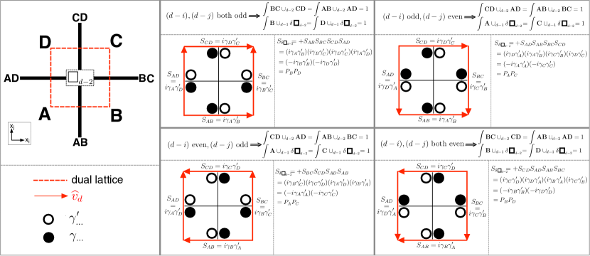
Figure 7: Various cases to check in the proof of Lemma 6. (Left) $\delta\boldsymbol{{\mathord{{\scalerel*{\Box}{t}}}}}_{d-2}$ defines a loop on the dual lattice in the $x_{i},x_{j}$ plane going between four $d$-hypercubes, ranging between ${\mathord{{\scalerel*{\Box}{t}}}}_{d}=A,B,C,D$ in counter-clockwise order. The four $(d-1)$-hypercubes $AB,BC,CD,AD$ are labeled according to the $d$-hypercubes they border. We refer to $\{{\bf A},{\bf B},{\bf C},{\bf D}\}$ and $\{{\bf AB},{\bf BC},{\bf CD},{\bf AD}\}$ as the indicator cochains on the respective hypercubes. The vector $\widehat{v}_{d}$ as described in Appendix LABEL:app:framingsOfCurvesAndWindings is a useful reference. (Right) The four cases of $(d-i),(d-j)$ being even/odd are checked. The nonzero integrals used to define $S_{\delta\boldsymbol{{\mathord{{\scalerel*{\Box}{t}}}}}_{d-2}}$ and in the Lemma are shown in each case, together with the algebra verifying the equalities.

Now, we only have four cases to verify depending on whether $i,j$ are even/odd. These four cases are analyzed in Figure 7. ∎

VI.2 Gu-Wen ‘Grassmann Integral’

VI.2.1 Definition using winding numbers

We start by explaining the how to give the “winding number” based defintion of the Grassmann integral $\sigma(\alpha)$. First we’ll briefly talk about the case where $\alpha$ is dual to a single closed curve on the dual lattice, which is described in more detail in the Appendix LABEL:app:framingsOfCurvesAndWindings. Then, we’ll talk about how to extend the definition to more general $\alpha$.

Suppose $L$ is a cochain defining a set of dual edges that define a simple, non-self-intersecting, closed curve on the dual lattice. The main idea is that there’s a canonical framing of the curve and thus a canonical way to define an induced spin structure on the framed curve. First, the space $\mathbb{R}^{d}$ is endowed with a ‘background framing’ consisting of the frame used to define the $\cup_{m}$ products via the thickening/shifting prescription. The curve itself is endowed with a framing given by the first $(d-2)$ vector fields of the frame used to define the $\cup_{m}$ products via the thickening/shifting prescription; this corresponds to the ‘shared framing’ discussed in Appendix LABEL:app:framingsOfCurvesAndWindings. Then, the induced spin structure on the curve can be computed in terms of the number of times the other two vectors of the background frame wind with respect to the tangent of the curve after projecting away these ‘shared framing’ directions. Call this winding number ‘wind$(L)$’. Then, the induced spin structure will be periodic if wind$(L)$ is even and it’ll be anti-periodic if wind$(L)$ is odd. Then, we’ll define $\sigma(L)$ for such loops as:

$$\sigma(L):=-(-1)^{\text{wind(L)}}=\begin{cases}1\text{ if anti-periodic}\\ -1\text{ if periodic}\end{cases}.$$ (46)

Now we want to extend this definition for more general closed $\alpha$. For such $\alpha$, its dual will be a sum over closed loops: $\alpha=L_{1}+\cdots+L_{k}$. As such, we would like to define $\sigma(\alpha)$ as a product of the $\sigma(L)$ the loop decomposition:

$$\sigma(\alpha):=\prod_{i=1}^{k}\sigma(L_{k})=(-1)^{\text{\# of loops}}\prod_{i=1}^{k}(-1)^{\text{wind}(L)}.$$ (47)

However, a priori the specific loop decomposition $\alpha=L_{1}+\cdots+L_{k}$ is ambiguous because the dual hypercubic lattice is a $2d$-valent graph. The way to deal with this, as in [T20], is to introduce a trivalent resolution of the dual 1-skeleton, so that any closed loop configuration would be endowed with a unique decomposition into distinct loops. The trivalent resolution we use is depicted in Fig. 8. For comparison, we also give a trivalent resolution that can be used in the simplicial case to define $\sigma$.

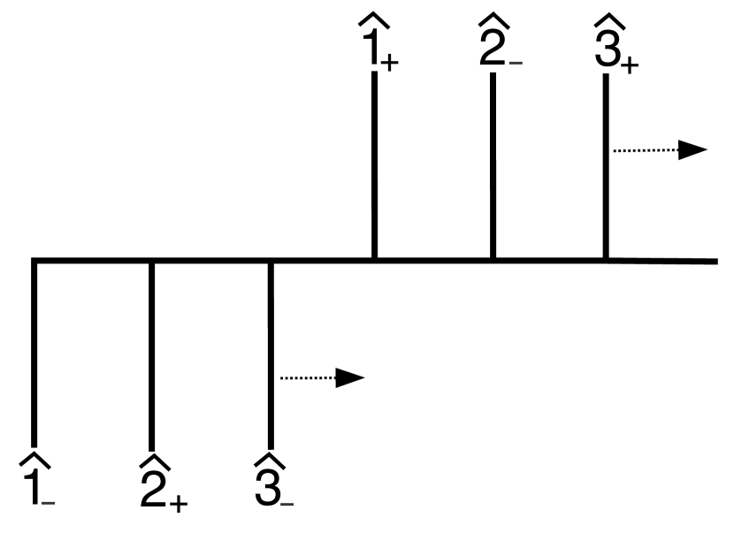
Figure 8: (Left) Trivalent resolution for the dual 1-skeleton on a simplex $\braket{0\cdots d}$, where $\hat{\imath}$ is the cell dual to $\braket{0\cdots\hat{\imath}\cdots d}$. (Right) Trivalent resolution for the dual hypercubic lattice in a single $d$-hypercube, where $\hat{\imath}_{\pm}$ refers to the dual cell pointing in the $\pm x_{i}$ direction relative to the center.

This function with the given trivalent resolution turned out to satisfy the quadratic refinement

$$\sigma(\alpha)\sigma(\beta)=\sigma(\alpha+\beta)(-1)^{\int\alpha\cup_{d-2}\beta}.$$ (48)

The argument for this is essentially the same as the argument in [T20], so we only briefly talk about it here. Quadratic refinement is a statement about how the windings of the collections of loops dual to $\alpha,\beta$ change when they reconnect and recombine in $\alpha+\beta$. This property is well-known in $d=2$ [johnson1980] where the $\int\alpha\cup_{d-2}\beta$ factor reduces to the intersection number $\int\alpha\cup\beta$ between $\alpha^{\vee},\beta^{\vee}$. In addition, one can use the thickening and shifting prescription of the higher-cup products to reduce the picture to project away the ‘shared framing’ directions and reduce the picture to $d=2$. Then, the $\int\alpha\cup_{d-2}\beta$ factor reduces to the intersection number of the curves in a ‘projected’ picture.

We also mention a subtlety that the particular trivalent resolution use is important in determining how the fermion lines reconnect with each other, and that not every trivalent resolution will work to reproduce quadratic refinement (although there are many that do work). In Fig. 8, we gave an example of resolutions that work in the simplicial case. It’s also interesting to compare our trivalent resolution to Fig. LABEL:fig:windingsGeneralDimensions in the Appendix were we draw a projected version of the dual 1-skeletons and vector fields in illustrating how to compute the windings.

Also, one can show that the values are all $+1$ on elementary loops dual to coboundaries of indicators ${\mathord{{\scalerel*{\Box}{t}}}}_{d-2}$ on a single $(d-2)$-simplex:

$$\sigma(\delta\boldsymbol{{\mathord{{\scalerel*{\Box}{t}}}}}_{d-2})=+1.$$ (49)

In the simplicial case, the formula was actually $\sigma(\delta{\bf\Delta}_{d-2})=(-1)^{w_{2}({\bf\Delta}_{d-2})}$ for indicator cochains ${\bf\Delta}_{d-2}$ and $w_{2}$ being the chain-representative dual to the second Stiefel-Whitney class. The geometric reason that these are all $+1$ here is that the background vector fields used to define the $\cup_{d-2}$ products are constant, so won’t have any singularities, thus $w_{2}\equiv 0$ for us.

Quadratic refinement and the values on elementary loops in Eqs. (48,49) actually fix the values of $\sigma(\delta\lambda)$ on all coboundaries $\delta\lambda$ (see [GK16]). In particular, we’ll have:

$$\sigma(\delta\lambda)=(-1)^{\int\lambda\cup_{d-4}\lambda+\lambda\cup_{d-3}\delta\lambda}.$$ (50)

And since $\mathbb{Z}^{d}$ is a trivial cell structure, this would actually tell us all values of $\sigma(\alpha)$. However, the constructions for $\sigma$ still make sense if we compactify the hypercubic lattice, say into a torus, and the values on nontrivial loops are not fixed in a similar way.

VI.2.2 Definition using Grassmann variables

While the above does produce a function $\sigma(\alpha)$, it would be nice if one could produce the same function $\sigma(\alpha)$ using Grassmann variables in the spirit of [guWen2014Supercohomology, GK16]. In fact we can produce a function that does exactly that.

For a cochain $\alpha\in C^{d-1}(\text{cubical complex},\mathbb{Z}_{2})$, define $\sigma^{\text{gr}}(\alpha)$ as follows:

$$\sigma^{\text{gr}}(\alpha)=\int\prod_{e|\alpha(e)=1}d\theta_{e}d{\bar{\theta}_{e}}\prod_{c}u(c)$$ (51)

where for each hypercube $c$, $u(c)$ is a product of Grassmann variables of $\theta_{e}$ or $\bar{\theta}_{e}$ of the edges $e\in c$. We’ll define $u(c)$ differently depending on when $d$ is even or odd:

$$u(c)=\begin{cases}\theta_{\hat{1}_{-}}^{\alpha(\hat{1}_{-})}\theta_{\hat{2}_{+}}^{\alpha(\hat{2}_{+})}\theta_{\hat{3}_{-}}^{\alpha(\hat{3}_{-})}\cdots{\bar{\theta}}_{\hat{1}_{+}}^{\alpha(\hat{1}_{+})}{\bar{\theta}}_{\hat{2}_{-}}^{\alpha(\hat{2}_{-})}{\bar{\theta}}_{\hat{3}_{+}}^{\alpha(\hat{3}_{+})}\cdots\text{ if }d\text{ even}\\ \cdots\theta_{\hat{3}_{+}}^{\alpha(\hat{3}_{+})}\theta_{\hat{2}_{-}}^{\alpha(\hat{2}_{-})}\theta_{\hat{1}_{+}}^{\alpha(\hat{1}_{+})}\cdots{\bar{\theta}}_{\hat{3}_{-}}^{\alpha(\hat{3}_{-})}{\bar{\theta}}_{\hat{2}_{+}}^{\alpha(\hat{2}_{+})}{\bar{\theta}}{\hat{1}_{-}}^{\alpha(\hat{1}_{-})}\text{ if }d\text{ even}\end{cases}.$$ (52)

Here, the notation $\theta_{\hat{\imath}_{\pm}}^{\alpha(\hat{\imath}_{\pm})}$ or ${\bar{\theta}}_{\hat{\imath}_{\pm}}^{\alpha(\hat{\imath}_{\pm})}$ means we include the Grassmann variable $\theta$ or ${\bar{\theta}}$ associated to the edge $\hat{\imath}_{\pm}$ if $\alpha(\hat{\imath}_{\pm})=1$, i.e. if that edge is included in the cochain. See Fig. 9 for a depiction of the Grassmann assignments.

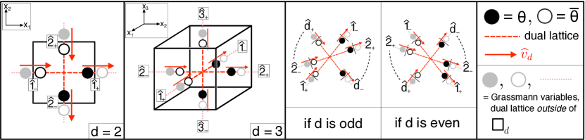
Figure 9: Assignment of Grassmann variables in a single ${\mathord{{\scalerel*{\Box}{t}}}}_{d}$ used in the definition of $\sigma^{\text{gr}}(\alpha)$ relative to the dual 1-skeleton and the $\widehat{v}_{d}$ vector (see Appendix LABEL:app:framingsOfCurvesAndWindings). A solid, open circle represents a placement of $\theta,\bar{\theta}$ respectively and the red dashed line is the dual 1-skeleton. The grayed circles and gray-red line represent the analogous quantities outside of ${\mathord{{\scalerel*{\Box}{t}}}}_{d}$.

Note that the assignment of Grassmann variables on edges mimics the assignments of Majorana operators of the exact bosonization in the sense that $\theta,\bar{\theta}$ variables occur in the same configurations as $\gamma,\gamma^{\prime}$ respectively (e.g. compare Figs. 6,7 to Fig. 9). Later on, in Sec. LABEL:sec:fermionicToricCode, we’ll actually connect $\sigma(f)$ to the exact bosonization in how it shows up in amplitudes of ground state of the ‘fermionic toric code’.

It ends up that $\sigma^{\text{gr}}(\alpha)$ literally equals the winding-based definition $\sigma(\alpha)$. We don’t reproduce the proof here but briefly describe it and how to map this hypercubic case onto a proof in an Appendix of [TKBB2021anomalies], which shows the analogous statement in the simplicial case. First, note that the order of the Grassmann variables is the same order as the edges that appear in the trivalent resolution Fig. 8 going from left to right. This can be used to show that both $\sigma(\alpha)$ and $\sigma^{\text{gr}}(\alpha)$ can be decomposed into products over the same set of loops that the dual of $\alpha$ gets decomposed into. Then, one has to check that indeed $\sigma(L)$ and $\sigma^{\text{gr}}(L)$ match on any cocycle $L$ dual to a single loop which can be done via some case-work and an inductive argument on the number of pairs of partial windings that occur throughout the loop. The map to the proof in [TKBB2021anomalies] can be guessed by matching orders of dual edges in Fig. 8, where the trivalent resolutions used for the simplicial and hypercubic cases are shown side-by-side. In particular, the proof in $d$ dimensions for the hypercubic case maps onto the proof in $(2d-1)$ dimensions in the simplicial case.

VII Construction of lattice models

Given a $(d+1)$-dimensional action $S_{d+1}$ for some space-time topological action for some theory, the ground-state wavefunction $\ket{\Psi}$ of the theory on a $d$-dimensional spatial manifold $M$ can be constructed as:

$$\braket{\Phi}{\Psi}\propto Z(\Phi)=\sum_{\text{fields}}\exp{\Big{(}2\pi i\cdot S_{d+1}(\text{fields};\Phi)\Big{)}}$$ (53)

where $\Phi$ is some state in the microscopic boundary Hilbert space that represents the boundary conditions of the topological action. Here, the partition function $Z(\Phi)$ is defined as a sum over some background ‘fields’ compatible with boundary conditions, and the ‘action’ $S_{d+1}(\text{fields};\Phi)$ depends on the boundary conditions $\ket{\Phi}$ and this background field $\Phi$.

A Hamiltonian formulation, or lattice model, of a topological action is a gapped Hamiltonian that admits $\ket{\Psi}$ as a ground-state. Well-known examples of such a correspondence are the Turaev-Viro/Levin-Wen [turaevViro1992, levinWen2005] and Crane-Yetter/Walker-Wang [craneYetter1993, walkerWang2012] correspondence which give path-integral/Hamiltonian correspondences for (resp.) (2+1)-$d$ and (3+1)-$d$ TQFTs related to tensor categories.

To construct a $d$-dimensional Hamiltonian out of a $(d+1)$-dimensional path integral, one needs to consider the ground states of the manifold on a triangulated surface with boundary. In general, such a ground state will be a superposition over all possible boundary conditions, with amplitudes being proportional to the path integral evaluated in the presence of the boundary conditions. For example, the Levin-Wen and Walker-Wang models are paradigmatic examples of ‘string net’ models where the ground states on a spatial manifold are configurations of strings with various colors with certain rules for branching at trijunctions. A basis of ground states is in correspondence with equaivalence classes of valid string-net configurations that can be transformed into each other via some set of local moves. Such a ground state will be a sum over all configurations in the equivalence class, and each local move gives a relationship between the amplitudes of these configurations. In the space-time path-integral, these string-nets are actually configurations of two-dimensional sheets that restrict to a string-net on the spatial boundary.

One way to construct such a Hamiltonian with such a ground state, is to consider one with two kinds of mutually commuting terms. The first kind are called ‘charge terms’ (often called ‘star terms’) which enforce certain constraints on what kinds of states are allowed in the ground state. In string-net states, these enforce the branching rules. The ‘flux terms’ (often called ‘plaquette terms’ in the context of string-net models) give the relations between amplitudes of configurations allowed by local moves. If all these terms mutually commute, then one can find the ground states exactly. And, a basis of grounds state is the equivalence classes of possible configurations modulo local moves.

Of particular interest to us are actions that can be written as a sum over cochains or cocycles. In particular, we’ll have that general states can look like $\ket{\Phi_{1},\cdots,\Phi_{n}}$ for cochains $\{\Phi_{1},\cdots,\Phi_{n}\}$, and states appearing with nonzero amplitudes in a ground state $\ket{\Psi}$ will require a closed-cochain condition, that each $\delta\Phi_{k}=0$ if $\braket{\Phi}{\Psi}\neq 0$. This condition will correspond to the charge terms.

The strategy to derive flux terms from a space-time action involves considering cochains $\{\Phi_{k}\}$ and their ground state amplitudes on a topologically trivial manifold, so that each $\Phi_{k}=\delta\tilde{a}_{k}$ is a coboundary. Generally on trivial manifolds, we will be able to derive exact expressions for $\braket{\{\delta\tilde{a}_{k}\}}{\Psi}$ in terms of the $\tilde{a}_{k}$. Then, we’ll show that the changes in amplitudes between $\braket{\{\delta\tilde{a}_{k}\}}{\Psi}$ and $\braket{\{\delta\tilde{a}_{k}+\delta\lambda_{k}\}}{\Psi}$ for indicator cochains $\lambda_{k}$ only depend on the $\delta\tilde{a}_{k}=\Phi_{k}$, and thus give local expressions for local changes in amplitudes.

And again, one would be able to derive the most general ground state on a manifold by considering the space of cocycle configurations modulo local changes, which in our examples will be in correspondence with cohomology classes, which by definition are cocycles modulo local changes.

VII.1 Warmup: $\mathbb{Z}_{n}$ toric code in arbitrary dimensions

We start by revewing the simplest example of such an action is the so-called ‘toric code’ following discussions in [BGK17, kapustinThorngren2017]. We start by reviewing the standard $\mathbb{Z}_{2}$ $(2+1)$D toric code and at the end note how this action generalizes to higher dimensions and $\mathbb{Z}_{n}$ coefficients, giving similar models.

The toric code’s space-time partition function can be expresssed as a sum over $\mathbb{Z}_{2}$ cochains $a\in C^{1}(M,\mathbb{Z}_{2})$ and chains $b\in C_{2}(M,\mathbb{Z}_{2})$ with action:

$$S_{t.c.}=\frac{1}{2}\int_{M^{2+1}}(a)(\partial b)$$ (54)

where $\int(a)(\partial b)$ gives the cochain-chain pairing $C^{1}(M,\mathbb{Z}_{2})\times C_{1}(M,\mathbb{Z}_{2})\to\mathbb{Z}_{2}$. For us, we consider boundary conditions of wavefunctions on the manifold as ${\left.\kern-1.2pta\vphantom{\big{|}}\right|_{\partial M}},{\left.\kern-1.2ptb\vphantom{\big{|}}\right|_{\partial M}}$. Actually for us, the ${\left.\kern-1.2ptb\vphantom{\big{|}}\right|_{\partial M}}$ represent ‘electric excitations’ above the ground state corresponding to electric-particle excitations, and we will set ${\left.\kern-1.2ptb\vphantom{\big{|}}\right|_{\partial M}}=0$. Note that our microscopic boundary Hilbert space is a tensor product of two-state systems $\{\ket{0}_{e},\ket{1}_{e}\}$ on each edge $e$ (or equivalently dual edge $e^{\vee}$) on the boundary 2D triangulation, and a state on the boundary corresponds to a boundary condition ${\left.\kern-1.2pta\vphantom{\big{|}}\right|_{\partial M}}(e)=\Phi(e)\in\{0,1\}$ for each edge.

Note that by Stoke’s theorem, above action reduces to

$$\begin{split}S_{t.c.}&=\frac{1}{2}\int_{M}(a)(\partial b)=\frac{1}{2}\int_{M}(\delta a)(b)+\frac{1}{2}\int_{\partial M}(a)(b)\\ &=\frac{1}{2}\int_{M}(\delta a)(b)\end{split}$$ (55)

where the first equality is an integration-by-parts and the second equality uses ${\left.\kern-1.2ptb\vphantom{\big{|}}\right|_{\partial M}}=0$. Note that the partition function associated to the above action will give a ground-state wavefunction

$$\begin{split}\braket{\Phi}{\Psi}\propto Z_{t.c.}(\Phi)=\sum_{\begin{subarray}{c}a\in C^{1}(M,\mathbb{Z}_{2})\,,\,{\left.\kern-1.2pta\vphantom{\big{|}}\right|_{\partial M}}(e)=\Phi(e)\\ b\in C_{2}(M,\mathbb{Z}_{2})\end{subarray}}(-1)^{\int(\delta a)(b)}.\end{split}$$ (56)

Note that summing over $b$ above gives that the amplitude $\braket{\Phi}{\Psi}$ is zero unless $\delta a=0$ everywhere throughout the 3-manifold $M$. This means that $a$ must be dual to closed worldsheets in $M$ that restrict to closed-loop configurations on $\partial M$, thus any nonzero amplitude in the $\ket{\Psi}$ wavefunction is associated to a closed-loop configuration on the dual cellulation of $\partial M$. This means that $b$ acts as a Lagrange multiplier, and ‘integrating it out’ enforces $\delta a=0$ in all nonzero amplitudes. This general feature of a Lagrange multiplier will generally apply in all situations we consider, and in the future we’ll often write the partition functions directly as sums over closed cochains.

A consequence is that the sum above reduces to

$$Z_{t.c.}(\Phi)=|C_{2}(M,\mathbb{Z}_{2})|\sum_{a\in C^{1}(M,\mathbb{Z}_{2})|\delta a=0}1=|C_{2}(M,\mathbb{Z}_{2})||Z^{1}(M,\mathbb{Z}_{2})|$$ (57)

which is a constant positive number for each $\Phi$. As such, we can write the full ground-state wavefunction on a simply-connected spatial manifold $N$ as:

$$\ket{\Psi}\propto\sum_{\tilde{a}\in C^{1}(N,\mathbb{Z}_{2})}\ket{\delta\tilde{a}}$$ (58)

where $\ket{\delta\tilde{a}}$ is the state with respect to the boundary conditions $\Phi=\delta\tilde{a}$, or equivalently, $\Phi(e)=(\delta\tilde{a})(e)$.

As such, the toric code is one of the simplest ‘topological orders’ because the ground-state wavefunction on a simply connected space is a sum over all closed loop configurations weighted with the same amplitude. In particular, the local constraint on these wavefunction amplitudes is trivial. Letting ${\bf v}\in C^{0}(N,\mathbb{Z}_{2})$ be an indicator cochain that’s nonzero on only one vertex, we’ll have:

$$\braket{\Phi+\delta{\bf v}}{\Psi}=\braket{\Phi}{\Psi}.$$ (59)

On a non-simply connected space, it is precisely this local constraint that we take to be the definition of the toric-code topological order. One consequence of this is that for any closed spatial manifold $N$ there are really $|H_{1}(N,\mathbb{Z}_{2})|$ independent wavefunctions $\ket{\Psi}$ that satisfy the above constraint, which correspond exactly to the $\mathbb{Z}_{2}$ functions on cohomology classes.

Now, we’re in a position to describe the toric code Hamiltonian. We’ll express the Hamiltonian in terms of the dual cellulation so that faces $f$ of the original cellulation are dual to vertices $f^{\vee}$ on the dual, and vertices $v$ of the original cellulation are dual to faces $v^{\vee}$

$$\begin{split}H_{t.c.}=-\sum_{f^{\vee}\in\begin{subarray}{c}\text{dual}\\ \text{vertices}\end{subarray}}U^{t.c.}_{f^{\vee}}-\sum_{v^{\vee}\in\begin{subarray}{c}\text{dual}\\ \text{faces}\end{subarray}}W^{t.c.}_{v^{\vee}}\text{, where}\\ U^{t.c.}_{f^{\vee}}:=\prod_{e^{\vee}\supset f^{\vee}}Z_{e^{\vee}},\quad\quad W^{t.c.}_{v^{\vee}}:=\prod_{e^{\vee}\subset v^{\vee}}X_{e^{\vee}}.\end{split}$$ (60)

Here, $e^{\vee}\supset f^{\vee}$ are all the (dual) edges containing the vertex $f^{\vee}$, and $e^{\vee}\subset v^{\vee}$ are the (dual) edges at the boundary of $v^{\vee}$. And, in the basis $\{\ket{0}_{e^{\vee}},\ket{1}_{e^{\vee}}\}$ of each dual edge, we have $Z_{e^{\vee}}=\begin{pmatrix}1&0\\ 0&-1\end{pmatrix}$ and $X_{e^{\vee}}=\begin{pmatrix}0&1\\ 1&0\end{pmatrix}$. Note that each term $U^{t.c.},W^{t.c.}$ in the Hamiltonian commute, which means that the above is a local commuting projector Hamiltonian. As such, any ground state of $H_{t.c.}$ is in the shared ground state of each term $-U^{t.c.}_{f^{\vee}}$ and $-W^{t.c.}_{v^{\vee}}$.

The first set of ‘star terms’ enforce that $U^{t.c.}_{f^{\vee}}\ket{\Psi}=\ket{\Psi}$. As such, let $\Phi\in C^{1}(M,\mathbb{Z}_{2})$ be such that $\braket{\Phi}{\Psi}\neq 0$. Then,

$$\bra{\Phi}U^{t.c.}_{f^{\vee}}\ket{\Psi}=\bra{\Phi}\prod_{e^{\vee}\supset f^{\vee}}Z_{e^{\vee}}\ket{\Psi}=\braket{\Phi}{\Psi}$$ (61)

while also

$$\ket{\Phi}=\prod_{e^{\vee}\supset f^{\vee}}Z_{e^{\vee}}\ket{\Phi}=(-1)^{(\delta\Phi)(f)}\ket{\Phi}.$$ (62)

The above two together require that $\delta\Phi\equiv 0$, so that $\Phi$ is a cocycle.

The second set of ‘flux terms’ enforce that each $W^{t.c.}_{v^{\vee}}\ket{\Psi}=\ket{\Psi}$, so that if $\braket{\Phi}{\Psi}\neq 0$, then

$$\bra{\Phi}W^{t.c.}_{v^{\vee}}\ket{\Psi}=\bra{\Phi}\prod_{e^{\vee}\subset v^{\vee}}X_{e^{\vee}}\ket{\Psi}=\braket{\Phi}{\Psi}$$ (63)

Also note that

$$\prod_{e^{\vee}\subset v^{\vee}}X_{e^{\vee}}\ket{\Phi}=\ket{\Phi+\delta{\bf v}}$$ (64)

Note that the above two equations exactly correspond to the local constraints Eq. (59) for each $v$.

In general dimension $d$, we’ll have that the toric code looks quite similar. We can write down essentially the same $(d+1)$ dimensional action

$$S_{t.c.}=\frac{1}{2}\int_{M^{d+1}}(a)(\partial b)$$ (65)

for the toric code, except where now the partition functions will sum over $a\in C^{d-1}(M,\mathbb{Z}_{2})$ with a Lagrange multiplier $b\in C_{d}(M,\mathbb{Z}_{2})$ that now sums over $d$-chains to enforce $\delta a=0$. And in the same way, we can impose boundary conditions $\Phi$ that give the restrictions of $a$ onto the boundary of the manifold, and we’d get again

$$Z_{t.c.}(\Phi)=|C_{d}(M,\mathbb{Z}_{2})|\sum_{a\in C^{1}(M,\mathbb{Z}_{2})|\delta a=0}1=|C_{d}(M,\mathbb{Z}_{2})||Z^{d-1}(M,\mathbb{Z}_{2})|$$ (66)

so that amplitudes of a ground state wave-function would be a sum over closed loop configurations on the dual lattice all weighted with equal positive amplitudes.

And again, one can engineer an entirely analogous Hamiltonian

$$\begin{split}H_{t.c.}=-\sum_{({\mathord{{\scalerel*{\Box}{t}}}}_{d})^{\vee}\in\begin{subarray}{c}\text{dual}\\ \text{vertices}\end{subarray}}U^{t.c.}_{({\mathord{{\scalerel*{\Box}{t}}}}_{d})^{\vee}}-\sum_{({\mathord{{\scalerel*{\Box}{t}}}}_{d-2})^{\vee}\in\begin{subarray}{c}\text{dual}\\ \text{2-cells}\end{subarray}}W^{t.c.}_{({\mathord{{\scalerel*{\Box}{t}}}}_{d-2})^{\vee}}\text{, where}\\ U^{t.c.}_{({\mathord{{\scalerel*{\Box}{t}}}}_{d})^{\vee}}:=\prod_{({\mathord{{\scalerel*{\Box}{t}}}}_{d-1})^{\vee}\subset({\mathord{{\scalerel*{\Box}{t}}}}_{d})^{\vee}}Z_{({\mathord{{\scalerel*{\Box}{t}}}}_{d-1})^{\vee}},\quad\quad W^{t.c.}_{({\mathord{{\scalerel*{\Box}{t}}}}_{d-1})^{\vee}}:=\prod_{({\mathord{{\scalerel*{\Box}{t}}}}_{d-1})^{\vee}\supset({\mathord{{\scalerel*{\Box}{t}}}}_{d-2})^{\vee}}X_{({\mathord{{\scalerel*{\Box}{t}}}}_{d-1})^{\vee}}.\end{split}$$ (67)

which with the charge terms $U$ enforce that the dual loop configurations are closed and the flux terms $W$ give local constraints so that all amplitudes so that in some ground sate, loop configurations in the same cohomology class are given equal amplitudes.

See Fig. 10 for a depiction of the terms in the Hamiltonian.

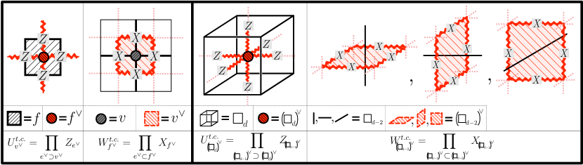
Figure 10: The different terms that occur in the $\mathbb{Z}_{2}$ toric code Hamiltonian. (Left) Two dimensions (Right) Three dimensions, with notation written for arbitarary dimensions.

The $\mathbb{Z}_{n}$ toric code will also be entirely analogous except it’s defined in terms of $\mathbb{Z}_{n}$ cochains rather than $\mathbb{Z}_{2}$ ones. We’ll define the action in $(d+1)$-dimensions as

$$S_{\mathbb{Z}_{n}t.c.}=\frac{1}{n}\int_{M^{d+1}}(a)(\partial b)$$ (68)

in terms of the arguments $a\in C^{1}(M,\mathbb{Z}_{n})$ and $b\in C_{d}(M,\mathbb{Z}_{n})$ with boundary conditions ${\left.\kern-1.2ptb\vphantom{\big{|}}\right|_{\partial M}}=0$. And again we impose boundary conditions $\Phi\in C^{1}(\partial M,\mathbb{Z}_{n})$ so that $\Phi={\left.\kern-1.2pta\vphantom{\big{|}}\right|_{\partial M}}$. And again, we’d have that

$$Z_{\mathbb{Z}_{n}t.c.}(\Phi)=|C_{d}(M,\mathbb{Z}_{n})|\sum_{a\in C^{1}(M,\mathbb{Z}_{n})|\delta a=0}1=|C_{d}(M,\mathbb{Z}_{n})||Z^{1}(M,\mathbb{Z}_{n})|$$ (69)

which would enforce that the ground state is a sum over all closed $\mathbb{Z}_{n}$-valued cochains.

And again, using the $\cup^{\prime}$ formalism over $\mathbb{Z}$ in Sec. V, it is straightforward to write down a Hamiltonian

$$H_{\mathbb{Z}_{n}t.c.}=-\sum_{({\mathord{{\scalerel*{\Box}{t}}}}_{d})^{\vee}\in\begin{subarray}{c}\text{dual}\\ \text{vertices}\end{subarray}}U^{\mathbb{Z}_{n}t.c.}_{({\mathord{{\scalerel*{\Box}{t}}}}_{d})^{\vee}}-\sum_{({\mathord{{\scalerel*{\Box}{t}}}}_{d-2})^{\vee}\in\begin{subarray}{c}\text{dual}\\ \text{2-cells}\end{subarray}}W^{\mathbb{Z}_{n}t.c.}_{({\mathord{{\scalerel*{\Box}{t}}}}_{d-2})^{\vee}}$$ (70)

for which the $U^{\mathbb{Z}_{n}t.c.}$ enforce that ground states are dual to closed $\mathbb{Z}_{n}$-cochains and for which $W^{\mathbb{Z}_{n}t.c.}$ give that cohomologous cochains are given equal weights in the wavefunctions.

VII.2 Three-fermion Walker-Wang model

In this section, we reproduce the lattice Hamiltonian for the 3-fermion Walker-Wang model [WW12, BCFV14]. This model is constructed from the 3-fermion braided fusion category, which is an abelian category with three nontrivial objects $\{e,m,\epsilon\}$ with fusion rules

$$e\times e=m\times m=\epsilon\times\epsilon=1\quad,\quad e\times m=\epsilon.$$ (71)

The $F$ symbols are trivial, and the $R$-symbols are given by

$$\begin{split}R_{\mu,\mu}&=-1,\text{ for all }\mu=e,m,\epsilon\\ R_{e,m}&=R_{m,\epsilon}=R_{\epsilon,e}=-1\\ R_{m,e}&=R_{\epsilon,m}=R_{e,\epsilon}=+1.\end{split}$$ (72)

The $R_{\mu\mu}=-1$ tell us that all the nontrivial particles are self-fermions.

A bulk action corresponding to this category can be found using the Crane-Yetter state-sum, whose Hamiltonian formulation is given by the corresponding Walker-Wang model. First, note that since the category is abelian, one can define the assignments of $e,m,\epsilon$ particles by two closed cochains $A,B\in Z^{2}(M^{4},\mathbb{Z}_{2})$. On a 2-cell, $A=B=0$ means placing an identity particle on the 2-cell, $A=1,B=0$ means place an $e$ particle, $A=0,B=1$ means place an $m$ particle, and $A=B=1$ means place an $e\times m=\epsilon$ particle. Then, the amplitudes of the bulk action are given by the $15j$ symbols of the assigments multiplied over all the 4-simplices. Writing out the $15j$ symbols shows that the amplitude to such an assignment of $A,B$ is exactly

$$S_{\text{3-fermion}}(A,B)=\frac{1}{2}\int_{M^{4}}A\cup A+B\cup B+A\cup B$$ (73)

since each $15j$ symbol on $\braket{01234}$ evaluates to $(-1)^{(A\cup A+B\cup B+A\cup B)(\braket{01234})}=(-1)^{A(012)A(234)+B(012)B(234)+A(012)B(234)}$. See also [KT14, HLS19, HJJ21] for more general actions of theories with 1-form or higher-group symmetries. On a closed manifold, one can evaluate a partition function on closed $M^{4}$ as

$$\begin{split}Z(M^{4})&\propto\sum_{A,B\in Z^{2}(M^{4},\mathbb{Z}_{2})}(-1)^{\int_{M}A\cup A+B\cup B+A\cup B}\\ &=\sum_{A,B\in Z^{2}(M^{4},\mathbb{Z}_{2})}(-1)^{\int(w_{2}+w_{1}^{2})\cup A+B\cup B+A\cup B}\\ &=\sum_{A,B\in Z^{2}(M^{4})}(-1)^{\int_{M^{4}}(w_{2}+w_{1}^{2}+B)\cup A+B\cup B}\\ &=(-1)^{\int_{M^{4}}(w_{2}+w_{1}^{2})\cup(w_{2}+w_{1}^{2})}=(-1)^{\int_{M^{4}}w_{2}^{2}+w_{1}^{4}}.\end{split}$$ (74)

Above, the second line used the Wu relation $\int_{M^{4}}A\cup A=\int_{M^{4}}(w_{2}+w_{1}^{2})\cup A$, and the fourth line notes that the sum over $A$ acts as a Lagrange multiplier setting $B=(w_{2}+w_{1}^{2})$. See also [barkeshli2019_nonorientable] for an alternate perspective on this result in terms of ‘anomaly indicators’.

VII.2.1 Bulk Hamiltonian

Now, we construct the Hamiltonian of this model and show that indeed it is the same as the one presented in Ref. [BCFV14, HFH18]. Note that we now need to consider two sets of $\mathbb{Z}_{2}$ degrees of freedom on the spatial manifold, $\Phi_{1},\Phi_{2}\in Z^{2}(N^{3},\mathbb{Z}_{2})$ that represent the boundary conditions of $A,B$ respectively. Now in our procedure, we consider the situation where both the bulk $M^{4}$ and boundary $N^{3}$ are topologically trivial, so that $A=\delta a$ and $B=\delta b$ in the bulk manifold. Then, with respect to the boundary conditions $\Phi_{1}={\left.\kern-1.2ptA\vphantom{\big{|}}\right|_{N}}={\left.\kern-1.2pt\delta a\vphantom{\big{|}}\right|_{N}},\Phi_{2}={\left.\kern-1.2ptB\vphantom{\big{|}}\right|_{N}}={\left.\kern-1.2pt\delta b\vphantom{\big{|}}\right|_{N}},$ the ground state $\ket{\Psi}$ on $N$ will have amplitudes

$$\begin{split}\braket{\Phi_{1},\Phi_{2}}{\Psi}&\propto(-1)^{\int_{M}(\delta a)\cup(\delta a)+(\delta b)\cup(\delta b)+(\delta a)\cup(\delta b)}\\ &=(-1)^{\int_{M}\delta(a\cup\delta a+b\cup\delta b+a\cup\delta b)}\\ &=(-1)^{\int_{N}a\cup\delta a+b\cup\delta b+a\cup\delta b}.\end{split}$$ (75)

From here, we compute the variations of these amplitudes with respect to $\Phi_{1}\to\Phi_{1}+\delta\lambda_{1}$ and $\Phi_{2}\to\Phi_{2}+\delta\lambda_{2}$ which correspond to $a\to a+\lambda_{1}$ and $b\to b+\lambda_{2}$ respectively. These have the form

$$\begin{split}\int_{N}&\big{(}(a+\lambda_{1})\cup\delta(a+\lambda_{1})+b\cup b+(a+\lambda_{1})\cup\delta b\big{)}-\big{(}a\cup a+b\cup b+a\cup\delta b\big{)}=\int_{N}a\cup\delta\lambda_{1}+\lambda_{1}\cup\delta a+\lambda_{1}\cup\delta\lambda_{1}+\lambda_{1}\cup\delta b\\ &=\int_{N}\delta a\cup\lambda_{1}+\lambda_{1}\cup\delta a+\lambda_{1}\cup\delta\lambda_{1}+\lambda_{1}\cup\delta b+\int_{\partial N}a\cup\lambda_{1},\end{split}$$ (76)

and

$$\begin{split}\int_{N}&\big{(}a\cup\delta a+(b+\lambda_{2})\cup(b+\lambda_{2})+a\cup\delta(b+\lambda_{2})\big{)}-\big{(}a\cup a+b\cup b+a\cup\delta b\big{)}=\int_{N}b\cup\delta\lambda_{2}+\lambda_{2}\cup\delta b+\lambda_{2}\cup\delta\lambda_{2}+a\cup\delta\lambda_{2}\\ &=\int_{N}\delta b\cup\lambda_{2}+\lambda_{2}\cup\delta b+\lambda_{2}\cup\delta\lambda_{2}+\delta a\cup\lambda_{2}+\int_{\partial N}(a+b)\cup\lambda_{2},\end{split}$$ (77)

where the second lines of each of the above use an integration-by-parts. For now, we’ll ignore these boundary integrals over $\partial N$ and interpret them later in the discussion of the boundary Hamiltonian.

At least for the bulk terms, we’ve expressed all the changes in amplitudes strictly in terms of $\Phi_{1}=\delta a$ and $\Phi_{2}=\delta b$, which means we have expressions for how the wavefunction amplitudes change with respect to local changes of the loop states. Our space of states will be two $\mathbb{Z}_{2}$ degrees $\{\ket{0}_{A,{\mathord{{\scalerel*{\Box}{t}}}}_{2}^{\vee}},\ket{1}_{A,{\mathord{{\scalerel*{\Box}{t}}}}_{2}^{\vee}}\}$ and $\{\ket{0}_{B,{\mathord{{\scalerel*{\Box}{t}}}}_{2}^{\vee}},\ket{1}_{B,{\mathord{{\scalerel*{\Box}{t}}}}_{2}^{\vee}}\}$ of freedom on each dual edge, dual to the 2-dimensional plaquettes that describe the cochains. And, there is the associated algebra of Pauli matrices $X_{A,{\mathord{{\scalerel*{\Box}{t}}}}_{2}^{\vee}},X_{B,{\mathord{{\scalerel*{\Box}{t}}}}_{2}^{\vee}}$ and $Z_{A,{\mathord{{\scalerel*{\Box}{t}}}}_{2}^{\vee}},Z_{B,{\mathord{{\scalerel*{\Box}{t}}}}_{2}^{\vee}}$.

First, the Hamiltonian will have charge (or star) terms $U^{\text{3-fermion}}_{{\mathord{{\scalerel*{\Box}{t}}}}^{\vee}_{3},\{A,B\}}$, at each vertex ${\mathord{{\scalerel*{\Box}{t}}}}^{\vee}_{3}$ dual to a 3-cube, that enforce $\delta\Phi_{1}=\delta\Phi_{2}=0$. Next, there will be flux (or plaquette) terms $W^{\text{3-fermion}}_{{\mathord{{\scalerel*{\Box}{t}}}}^{\vee}_{1},\{A,B\}}$ for each possible change of wave-function cochain $\Phi_{1}\to\Phi_{1}+\delta\boldsymbol{{\mathord{{\scalerel*{\Box}{t}}}}}_{1}$ or $\Phi_{2}\to\Phi_{2}+\delta\boldsymbol{{\mathord{{\scalerel*{\Box}{t}}}}}_{1}$ for $\boldsymbol{{\mathord{{\scalerel*{\Box}{t}}}}}_{1}\in C^{1}(N,\mathbb{Z}_{2})$ the indicator cochains representing changes in the different $\mathbb{Z}_{2}$ degrees of freedom. These together create a Hamiltonian

$$H^{\text{3-fermion}}=-\sum_{{\mathord{{\scalerel*{\Box}{t}}}}_{3}}U^{\text{3-fermion}}_{{\mathord{{\scalerel*{\Box}{t}}}}^{\vee}_{3},A}-\sum_{{\mathord{{\scalerel*{\Box}{t}}}}_{3}}U^{\text{3-fermion}}_{{\mathord{{\scalerel*{\Box}{t}}}}^{\vee}_{3},B}-\sum_{{\mathord{{\scalerel*{\Box}{t}}}}_{1}}W^{\text{3-fermion}}_{{\mathord{{\scalerel*{\Box}{t}}}}^{\vee}_{1},A}-\sum_{{\mathord{{\scalerel*{\Box}{t}}}}_{1}}W^{\text{3-fermion}}_{{\mathord{{\scalerel*{\Box}{t}}}}^{\vee}_{1},B}$$ (78)

whose terms are depicted in Fig. 11. Note that these terms match the previous 3-fermion Walker-Wang model construction [BCFV14] exactly.

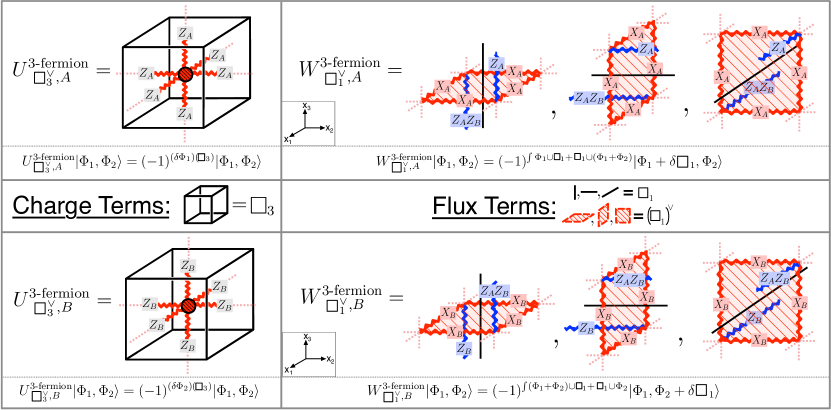
Figure 11: Terms in the Three-Fermion Walker-Wang model in terms of hypercubic cochain operations, following the flux terms Eqs. (76,77) and Fig. 4

VII.2.2 Boundary Hamiltonian

In the derivation of the bulk Hamiltonian above, a key step in getting the right wave-function amplitudes was an integration-by-parts on the second lines of Eqs. (76,77). However, the integration-by-parts left some boundary terms that would affect the required plaquette terms on the boundary.

Before deriving boundary terms for the Hamiltonian, it’s helpful to have a short digression on how to think about cochains in the presence of a boundary. Recall that in the discussion above, $a,b\in C^{1}(N,\mathbb{Z}_{2})$ are 1-cochains that are dual to two-dimensional sheets in the bulk, whereas $\delta a,\delta b\in Z^{2}(N,\mathbb{Z}_{2})$ are 2-cochains dual to one-dimensional lines. However the restrictions ${\left.\kern-1.2pt\{a,b\}\vphantom{\big{|}}\right|_{\partial N}}$ and ${\left.\kern-1.2pt\{\delta a,\delta b\}\vphantom{\big{|}}\right|_{\partial N}}$ to $\partial N$ will still be 1-cochains and 2-cochains respectively, which will instead be dual to 1-dimensional lines and 0-dimensional points on $\partial N$. This has the interpretation that the loop configurations associated to $\delta a$ in the bulk $N$ are continued onto some lines associated to $a$ on $\partial N$. See Fig. 12 for a depiction.

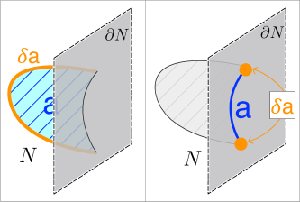
Figure 12: Here, $a\in C^{1}(N,\mathbb{Z}_{2})$ and $\delta a\in C^{2}(N,\mathbb{Z}_{2})$ are sheets and lines in the bulk manifold $N$. However restricted to $\partial N$, $a$ becomes a line that continues the bulk $\delta a$ and $\delta a$ on the boundary becomes the endpoints of the boundary line.

As such, in our Hamiltonian formulation, the lines of the string-net restricted to $\partial N$ will actually be represented by the cochain $a$ that represented the bulk sheets. In this section we consider wave-functions formed by the basis of all of the dual one-dimsional edges on $N,\partial N$, which would be represented by the Hilbert space

$$\mathcal{H}_{\text{3-fermion}}=\mathrm{span}\left(\Big{\{}\ket{\delta a,\delta b;{\left.\kern-1.2pta\vphantom{\big{|}}\right|_{\partial N}},{\left.\kern-1.2ptb\vphantom{\big{|}}\right|_{\partial N}}}\Big{|}a,b\in C^{1}(N,\mathbb{Z}_{2})\Big{\}}\right).$$ (79)

Another way to think of the boundary terms is to consider an ‘augmented’ lattice. For example, if we take $N$ to be the half of the hypercubic lattice, which is the full lattice restricted to one $x_{i}\leq 0$, then we could create an $N^{\text{aug}}$ by adding an extra ‘row’ of $x_{i}=1$ to the lattice and considering cochains on that augmented lattice. In addition, one needs to impose some boundary conditions that all cochains involving any coordinate with $x_{i}>0$ should be set to zero. Then, the cochains on $(N,\partial N)$ will be in one-to-one correspondence with cochains on $N^{\text{aug}}$ subject to the cochains vanishing if they involve $x_{i}>0$. This correspondence is illustrated in Fig. 13.

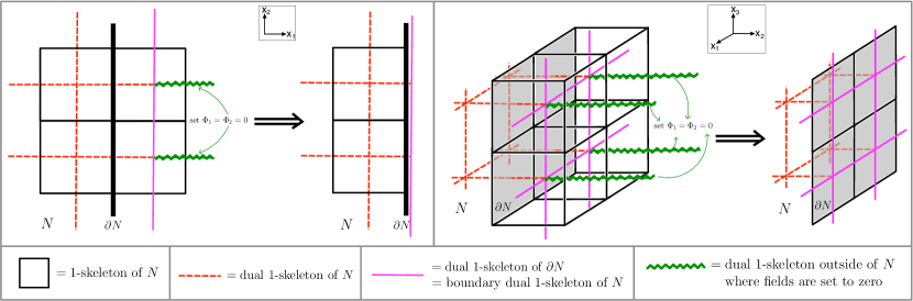
Figure 13: Cochains on $(N,\partial N)$ can be represented by augmenting $N$ by one extra row and considering cochains on the augmented lattice subject to boundary conditions of zero. In our case, we set the fields $\Phi_{1}\equiv\delta a=0$ and $\Phi_{2}\equiv\delta b=0$. (Left) The two-dimensional case. (Right) The three-dimensional case.

Now we are in a position to list out the boundary terms implied by the Eqs. (76,77). They are depicted in Fig. 14. They can be derived from similar considerations as the bulk terms we derived previously. The charge terms enforce that bulk and boundary lines are closed loops when added together.

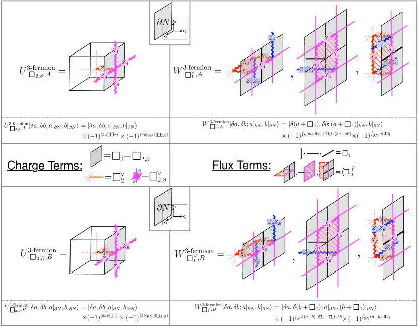
Figure 14: Boundary terms of the 3-fermion model subject to a termination in the $(x_{1},x_{3})$ plane. Here, we illustrate the ‘charge terms’ in terms of the squares ${\mathord{{\scalerel*{\Box}{t}}}}_{2,\partial}$ on $\partial N$.

We illustrated these terms in terms of the relevant cochains on $(N,\partial N)$. However, we note that we could just as well think of them as cochains on the augmented lattice $N^{\text{aug}}$; these terms are precisely the bulk terms of Fig. 11 subject to the boundary conditions $a=b=0$ outside of $N$.

In [HFH18], we note that essentially the same set of terms were found to be essentially the unique possible boundary terms for the 3-fermion model .

VII.2.3 Relation to Quantum Cellular Automaton (QCA)

In Ref. [HFH18], the 3-fermion Walker-Wang model is used to construct a quantum cellular automaton (QCA). To define the QCA, we need to modify the Hamiltonian such that all of the charge and terms are independent, that no product of such terms is the identity. In the current expression (78), the star terms and plaquette terms are not independent (one can check that the product of plaquette terms on faces of a cube is equal to a product of star terms). Ref. [HFH18] introduce the polynomial method and an algorithm to eliminate this redundancy. The final Hamiltonian contains only the plaquette terms expressed by polynomials, which can’t be visualized on the cubic lattice easily. In the following, we are going to use the $\cup_{1}$ product identity on (76) and (77) and get modified plaquette terms such that they are non-redundant and complete (able to generate original star terms and plaquette terms).

From (76) with $\lambda_{1}=\boldsymbol{{\mathord{{\scalerel*{\Box}{t}}}}}_{1}$ (the 1-cochain with value $1$ on the edge ${\mathord{{\scalerel*{\Box}{t}}}}_{1}$ and $0$ otherwise) on closed $N$ ($\partial N=0$), we have &∫_N δa ∪*□t_1 + *□t_1 ∪δa + *□t_1 ∪δ*□t_1 + *□t_1 ∪δb
= ∫_N δ*□t_1 ∪_1 δa + *□t_1 ∪δb, where we have used $\boldsymbol{{\mathord{{\scalerel*{\Box}{t}}}}}_{1}\cup\delta\boldsymbol{{\mathord{{\scalerel*{\Box}{t}}}}}_{1}=0$ and the recursive relation $\delta(\alpha\cup_{1}\beta)=\delta\alpha\cup_{1}\beta+\alpha\cup_{1}\delta\beta+\alpha\cup\beta+\beta\cup\alpha$. The new plaquette term is W’_*□t_1^∨, A = ∏_f—*□t_1 ∈∂f X_A,f ∏_f’ Z_A,f’^∫_N δ*□t_1 ∪_1 f’ ∏_f” Z_B,f”^∫_N *□t_1 ∪f”, or equivalently W’_*□t_1^∨, A