Band manipulation and spin texture in interacting moiré helical edges

Abstract

We develop a theory for manipulating the effective band structure of interacting helical edge states realized on the boundary of two-dimensional time-reversal symmetric topological insulators. For sufficiently strong interaction, an interacting edge band gap develops, spontaneously breaking time-reversal symmetry on the edge. The resulting spin texture, as well as the energy of the time-reversal breaking gaps, can be tuned by an external moiré potential (i.e., a superlattice potential). Remarkably, we establish that by tuning the strength and period of the potential, the interacting gaps can be fully suppressed and interacting Dirac points re-emerge. In addition, nearly flat bands can be created by the moiré potential with a sufficiently long period. Our theory provides an unprecedented way to enhance the coherence length of interacting helical edges by suppressing the interacting gap. The implications of this finding for ongoing experiments on helical edge states is discussed.

Introduction. – Moiré heterostructures, such as magic-angle twisted bilayer graphene, provide tunable platforms to realize novel interaction-driven phases Cao et al. (2018a, b); Yankowitz et al. (2019); Kerelsky et al. (2019); Lu et al. (2019); Jiang et al. (2019); Xie et al. (2019); Choi et al. (2019); Polshyn et al. (2019); Cao et al. (2020a); Polshyn et al. (2020); Serlin et al. (2020); Sharpe et al. (2019); Chen et al. (2019); Po et al. (2018); Xu and Balents (2018); Wu et al. (2018a); Xie and MacDonald (2020); Zhang et al. (2019); Lian et al. (2019); Wu et al. (2019); You and Vishwanath (2019); Kang and Vafek (2019); Bultinck et al. (2020a); Xie et al. (2020); Lian et al. (2021); Bernevig et al. (2021); Xie et al. (2021); Bultinck et al. (2020b); Wang et al. (2021a); Vafek and Kang (2020); Chen et al. (2021); Cea and Guinea (2020); Wang et al. (2021b); Wu and Das Sarma (2020); Alavirad and Sau (2020). Microscopically, these interaction-driven phenomena result from extremely flat bands that are created by the relative twist of two-dimensional (2D) low-energy Dirac cones to a magic angle Bistritzer and MacDonald (2011); Lopes dos Santos et al. (2012), so that many body interactions become significant. Recent proposals have extended this paradigm to other 2D materials Tang et al. (2020); Regan et al. (2020); Shimazaki et al. (2020); Wang et al. (2020); Tsai et al. (2019); Cao et al. (2020b); Burg et al. (2019); Shen et al. (2020); Liu et al. (2020); Pan et al. (2020); Zang et al. (2021), unconventional superconductors Can et al. (2021); Volkov et al. (2020), ultracold atoms in optical lattices González-Tudela and Cirac (2019); Luo and Zhang (2021), and acoustic metamaterials Gardezi et al. (2021). Engineering flat bands by tuning to a “magic angle” is quite general and may be induced by external quasiperiodic potentials and tunneling processes Fu et al. (2020a); Salamon et al. (2020a, b); Chou et al. (2020); Fu et al. (2020b) that can be extended to a “magic-continuum” Luo et al. (2021).

A moiré superlattice potential can also be used to control and manipulate a 2D Dirac cone on the surface of a topological insulator (TI), producing favorable conditions to realize interacting instabilities such as topological superconductivity or quantum anomalous Hall by enhancing the density of states Cano et al. (2021); Wang et al. (2021c). However, if the surface states are protected by time-reversal symmetry, the formation of a flat, gapped, miniband is topologically obstructed. Spontaneous symmetry breaking permits an interaction-driven gap, but an analysis of the strong coupling regime is lacking.

Figure 1: Setup and band structure manipulation. (a) Illustration of the setup. A 2D TI edge state is perturbed by an external periodic potential, $V(x)=w\cos(Qx)$. (b) For a weak repulsive interaction ($1/2<K<1$), the edge band is unaffected by the external potential. (c) For a strong repulsive interaction ($K<1/2$), interaction-induced gaps can open at both zero energy and finite energies. In addition, for particular $w$ and $Q$, the interaction-induced gap may vanish, resulting in a re-emergent gapless edge (middle figure). The gaps are labeled by $m$ corresponding to $E=mvQ/4$.

In this Letter, by focusing on the helical edge states of a 2D topological insulator, we utilize the power of bosonization to provide a clear theoretical demonstration of how strongly coupled interaction-driven phases emerge in moiré tuned topological edge states when time-reversal symmetry is spontaneously broken. In particular, we study the interplay between interactions and a moiré potential (specifically, a periodic potential in the continuum theory) on the 1D helical edge states of a 2D time-reversal-invariant topological insulator Kane and Mele (2005a, b); Bernevig and Zhang (2006); König et al. (2007); Roth et al. (2009); Knez et al. (2011); Du et al. (2015); Li et al. (2015); Du et al. (2017); Li et al. (2017); Tang et al. (2017); Wu et al. (2018b); Chen et al. (2018); Ugeda et al. (2018); Reis et al. (2017); Stühler et al. (2020), shown in Fig. 1(a). Distinct from previous works on the interaction-induced helical spin texture Sun et al. (2015) and RKKY induced orders in the external spins Hsu et al. (2018); Yevtushenko and Tsvelik (2018), we focus on the band dispersion of the strongly interacting edges, which can be manipulated by a time-reversal breaking gap at zero energy that develops due to interaction induced backscattering, i.e. umklapp processes Wu et al. (2006); Xu and Moore (2006) [as sketched in Fig. 1(b) and (c)]. We show systematically that the spin textures of the interacting gaps can be controlled by both the oscillation period Sun et al. (2015) and the amplitude of the periodic potential and exhibit a nontrivial structure. With the ability to manipulate the gaps in the band structure, we demonstrate that the edge band can be engineered such that re-emergent Dirac points and nearly flat bands can be realized. The re-emergence of the Dirac point at $E=0$ [Fig. 1(c)] indicates that the periodic potential can enhance the coherence length of the strongly interacting helical edge state, which is useful for ongoing experiments trying to observe topological insulator edge states in quantum wells Du et al. (2015); Li et al. (2015); Du et al. (2017); Li et al. (2017); Bubis et al. (2021). Our proposed set up depicted in Fig. 1(a) can also be realized in ultracold Fermi gases subjected to a two-dimensional spin orbit coupling Huang et al. (2016); Song et al. (2018), where the edge potential can be generated via an additional one-dimensional optical lattice.

Model. – The edge of a 2D time-reversal-invariant topological insulator is described by a 1D Dirac Hamiltonian perturbed by interaction and an inhomogeneous potentialKane and Mele (2005b); Wu et al. (2006); Xu and Moore (2006),

$$\hat{H}= \sum_{r=R,L}\int dx\left[v_{r}\psi_{r}^{\dagger}\left(-i\partial_{x}\psi_{r}\right)+V(x)\psi_{r}^{\dagger}(x)\psi_{r}(x)\right]$$

$$+ U\int dx:\left[e^{i\delta Gx}\left(\psi_{L}^{\dagger}\psi_{R}\right)^{2}+\text{H.c.}\right]+\hat{H}_{\text{LL}}$$ (1)

where $v_{r}=\pm v_{F}$ is the Fermi velocity for $r=R/L$ and $\hat{H}_{\text{LL}}$ denotes the forward scattering interactions Giamarchi (2004) whose precise form is not important here. In the above expressions $\psi_{R}$ ($\psi_{L}$) is the right-moving (left-moving) fermionic field, $V(x)$ is a spatially varying potential, $U$ encodes the interaction strength, $\delta G=4k_{F}-G$, $k_{F}$ is the Fermi wavevector, $G$ is a reciprocal lattice vector, and $:\mathcal{O}:$ denotes the normal ordering of $\mathcal{O}$. The right-moving and the left-moving fermions form a Kramers pair. Under time-reversal, the fermionic fields are transformed as: $\psi_{R}\rightarrow\psi_{L}$, $\psi_{L}\rightarrow-\psi_{R}$, and $i\rightarrow-i$. Thus, time-reversal symmetry forbids elastic single-particle backscattering (e.g., $\psi_{L}^{\dagger}\psi_{R}$), but long-wavelength forward scattering (e.g., $\psi_{R}^{\dagger}\psi_{R}$) is allowed. In the presence of Rashba spin orbit coupling, the time-reversal symmetric backscattering interaction [$U$ term in Eq. (Band manipulation and spin texture in interacting moiré helical edges)] can arise, and spin is no longer a good quantum number. We focus only on $G=0$ for simplicity, although the results do not rely on this assumption.

Thus, the interacting inhomogeneous helical edge can be described by $\hat{H}=\hat{H}_{0}+\hat{H}_{V}+\hat{H}_{U}+\hat{H}_{\text{LL}}$ Chou et al. (2018); Chou (2019). To study the interplay between interactions and an external periodic potential, we consider

$$V(x)=w\cos\left(Qx\right),$$ (2)

where $w$ controls the strength of the potential and $Q>0$ dictates the oscillation in space. We assume that $2\pi/Q$ is not commensurate with the 2D lattice constant $d$. We also assume that the edge physics does not change the bulk topological phase.

Commensurate-incommensurate transitions.– The interacting helical fermions can be mapped to an interacting bosonic problem Shankar (2017); Giamarchi (2004) with two bosonic fields ($\phi$ and $\theta$) that are related to the density and current operators of the original fermion degrees of freedom (see SM for a detailed discussion.) To incorporate the effect of the external potential, we perform a linear transformation, $\theta^{\prime}(x)=\theta(x)+\frac{Kw}{vQ}\sin(Qx)$, which yields the bosonized Hamiltonian

$$\hat{H}_{b}^{\prime}= \int dx\frac{v}{2\pi}\left[K\left(\partial_{x}\phi\right)^{2}+\frac{1}{K}\left(\partial_{x}\theta^{\prime}\right)^{2}\right]$$

$$\!-\tilde{U}\int\!dx\cos\!\left[4\theta^{\prime}(x)\!-\!\frac{4Kw}{vQ}\sin(Qx)\!+\!4k_{F}x\right],$$ (3)

where $v$ is the velocity of boson, $K$ is the Luttinger parameter, $\tilde{U}=U/(2\pi^{2}a^{2})$U_t , and $a$ is the ultraviolet length scale in the low-energy theory. We focus only on repulsive interactions, corresponding to $K<1$. Equation (3) is the starting point of our work.

In the absence of the external potential (i.e., $w=0$), the Hamiltonian in Eq. (3) maps to the Pokrovsky-Talapov model for the commensurate-incommensurate transition Pokrovsky and Talapov (1979); Giamarchi (2004). At the Dirac point (i.e., $k_{F}=0$), the model is commensurate, and the cosine term in Eq. (3) becomes relevant in the renormalization group sense, inducing a spectral gap for $K<1/2$ Wu et al. (2006); Xu and Moore (2006); Giamarchi (2004). For fillings that are sufficiently away from the Dirac point, the model is incommensurate, and the $\tilde{U}$ term is irrelevant, suggesting a Luttinger liquid behavior.

To study Eq. (3) with a nonzero $w$, we express the cosine term ($\tilde{U}$ term) as a Fourier series FT :

$$\cos\left[4\theta^{\prime}(x)-\frac{4Kw}{vQ}\sin(Qx)+4k_{F}x\right]$$

$$= \sum_{m=-\infty}^{\infty}|\tilde{F}_{m}|\cos\left[4\theta^{\prime}(x)+(4k_{F}-mQ)x+\chi_{m}\right],$$ (4)

where $\tilde{F}_{m}$ corresponds to the Fourier component of $\exp\left[i\frac{4Kw}{vQ}\sin(Qx)\right]$ and $\chi_{m}$ is the phase of $\tilde{F}_{m}$. Intuitively, Eq. (4) shows that the presence of the potential has reorganized the interaction into a series of backscattering processes with momentum $mQ$, which, in conjunction with the Luttinger parameter, can each open a gap in the excitation spectrum. If such a gap, labeled by $m$, opens, then time reversal symmetry on the edge must be spontaneously broken, lifting the topological obstruction to a gapped boundary. In the following, we investigate Eqs. (3) and (4) by adopting the analysis in Refs. Vidal et al. (1999, 2001), which considered a single cosine term ($w=0$ case) Pokrovsky and Talapov (1979); Giamarchi (2004), to the case with multiple cosine terms ($w\neq 0$ case). As we will show, the gapped edge states exhibit a nontrivial magnetic structure. Further, the magnitude of the gap can be tuned by the strength and period of the potential, allowing a gapless Dirac cone to be realized at special points in the phase diagram.

The commensuration condition for each $m$ [i.e. each cosine term in the summand of Eq. (4)] is $4k_{F}=mQ$. If this condition is satisfied, the $\tilde{F}_{m}$ term in Eq. (4) can open a band gap of size $2v\delta Q_{c}^{(m)}$ for sufficiently strong interaction ($K<1/2$), as shown in Fig. 2(a). The gapless state will be restored by sufficiently large incommensuration $|4k_{F}-mQ|>\delta Q_{c}^{(m)}$ as the integral over the cosine term in Eq. (3) for this $m$ will vanish. In general, the threshold of commensuration, $\delta Q_{c}^{(m)}$, is a complicated function of $\tilde{U}$, $w$ and $K$ Pokrovsky and Talapov (1979); Giamarchi (2004). If, for each $m$, $Q>4\delta Q_{c}^{(m)}$, then the interacting gaps in the TI edge spectrum are well separated and we can treat the summand of Eq. (4) as a collection of independent cosine terms. On the other hand, if $Q\leq 4\delta Q_{c}^{(m)}$, the cosine terms in Eq. (4) interfere with each other; shortly we will employ an exact mapping at $K=1/4$ to study this case.

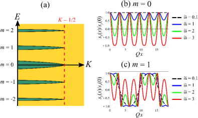
Figure 2: Phase diagram and spin texture of the time-reversal breaking order. (a) The phase diagram for $|Q|>4\delta Q_{c}^{(m)}$ based on bosonization analysis. The yellow region denotes the metallic phase. For $K<1/2$, time-reversal breaking gaps (green regions) can be induced by the interaction. The energy of the gap is $E=mvQ/4$ for an integer $m$. The half width of the gap is $v\delta Q_{c}^{(m)}$, as discussed in the main text. (b)-(c): Normalized $s_{y}(x)$ [Eq. (6)] as a function of $Qx$. The phase shift $\zeta_{m,N}$ is set to zero for convenience. (b) $m=0$. (c) $m=1$. We define the dimensionless parameter $\tilde{\omega}=\frac{2Kw}{vQ}$. In both figures, $\tilde{\omega}=0,1,2,3$ correspond to the black dashed lines, blue lines, green lines, and red lines respectively.

Interacting gaps and spin texture. – For a helical edge state with $K<1/2$, the commensurate cosine term (i.e., satisfying $|4k_{F}-mQ|<\delta Q_{c}^{(m)}$) in Eq. (4) becomes relevant, implying the formation of time-reversal breaking gaps at the energies $E(m)=mvQ/4$ labelled in Fig. 1(c). A phase diagram is illustrated in Fig. 2(a). Since the helical edge state is “spin-momentum locked,” the time-reversal breaking gaps carry nontrivial magnetic structures. We discuss the alternative charge picture in SM .

To understand the consequence of spin momentum locking on the magnetic texture of each gap we compute the spin densities $\langle s_{x}(x)\rangle$ and $\langle s_{y}(x)\rangle$ (see SM for definitions). When the backscattering interaction dominates (i.e., $K<1/2$ and commensurate), we employ a mean field approach: for each mode $m$ in Eq. (4), we solve for $\theta^{\prime}(x)$ by minimizing the corresponding cosine term and then use $\theta^{\prime}(x)=\theta(x)+\frac{Kw}{vQ}\sin(Qx)$ to compute the expectation values of $s_{x}$ and $s_{y}$, yielding

$$\langle s_{x}(x)\rangle\approx \frac{1}{\pi a}\sin\left[\frac{mQx}{2}-\frac{2Kw}{vQ}\sin(Qx)+\zeta_{m,N}\right],$$ (5)

$$\langle s_{y}(x)\rangle\approx \frac{1}{\pi a}\cos\left[\frac{mQx}{2}-\frac{2Kw}{vQ}\sin(Qx)+\zeta_{m,N}\right],$$ (6)

where $\zeta_{m,N}=\pi N-\chi_{m}/2$ is an unimportant phase factor with arbitrary integer $N$. The expressions in Eqs. (5) and (6) reduce to a single frequency oscillation Sun et al. (2015) in the limit $2Kw/(vQ)\ll 1$. Generically, the spin density wave (SDW) states manifest non-sinusoidal oscillations due to the potential in Eq. (2). As plotted in Figs. 2(b) and (c), the value of $w$ controls the spin texture of the time-reversal breaking order nontrivially, resulting in unusual spin order. In particular, the ferromagnetic order at $E=0$ (equivalently $m=0$) can be deformed to a qualitatively different finite-momentum SDW state in the presence of a sufficiently large $w$.

Luther-Emery theory and tunable band structure. – To go beyond the mean field approximation, we turn to the exact Luther-Emery refermionization mapping at $K=1/4$ Giamarchi (2004). The interacting bosonized Hamiltonian in Eq. (3) maps to a noninteracting massive fermion Hamiltonian:

$$\hat{H}_{b}\rightarrow\sum_{r=R,L}\int dx\left[\tilde{\Psi}_{r}^{\dagger}\left(-i\tilde{v}_{r}\partial_{x}+\tilde{V}(x)\right)\tilde{\Psi}_{r}-\tilde{M}_{r}\tilde{\Psi}^{\dagger}_{\bar{r}}\tilde{\Psi}_{r}\right]$$ (7)

where $\tilde{v}_{r}=\pm v$ for $r=R/L$ is the velocity of the Luther-Emery fermions, $\tilde{V}(x)=V(x)/2+vk_{F}/2$, $\tilde{M}_{r}=\pm iM$ for $r=R/L$, $M=U/(2\pi a)$, $\bar{r}$ denotes the opposite direction of $r$, and the Luther-Emery fermionic field is given by $\tilde{\Psi}_{R/L}=\frac{1}{\sqrt{2\pi a}}e^{i\left[\phi/2\pm 2\theta\right]}$. The mass term of the Luther-Emery fermions arises from the backscattering interaction [$U$ term in Eq. (Band manipulation and spin texture in interacting moiré helical edges)]. The Luther-Emery fields ($\Psi_{R}$ and $\Psi_{L}$) are not simply related to the physical low-energy fermions ($R$ and $L$). Nevertheless, we can extract information from the Luther-Emery theory such as the energy spectrum, density, and current Chou et al. (2018).

For the Luther-Emery fermions, the band gap induced by spontaneous time-reversal symmetry breaking is $2|M|$. The appearance of finite-energy gaps [see Figs. 1(c) and 2(a)] can be understood intuitively by the band folding due to $V(x)/2$ and second order perturbation theory in $V(x)/2$. Note that the gap opening condition corresponds to $4k_{F}-mQ=0$ with an integer $m$, which is consistent with the commensurate condition discussed previously.

In addition, controlling the magnitude of the periodic potential can close/reopen the zero-energy and finite-energy gaps. To see this analytically, we treat the periodic potential as a perturbation and compute the renormalized velocity and effective mass, which we find to be given by

$$\tilde{v}=vZ\left[1-\alpha^{2}+\alpha^{2}\frac{2v^{2}Q^{2}}{v^{2}Q^{2}+M^{2}}\right],\,\tilde{M}=MZ\left(1-\alpha^{2}\right),$$ (8)

respectively, where $Z=1/(1+\alpha^{2})$ is the wavefunction renormalization, and we have introduced a dimensionless coupling constant $\alpha^{2}=\frac{w^{2}}{8\left(v^{2}Q^{2}+M^{2}\right)}$. Remarkably, the Dirac mass can be renormalized to zero (i.e. $\tilde{M}=0$) when $\alpha=1$ , suggesting a Dirac point at $E=0$ and band inversion signalled by the change in sign of $\tilde{M}$. This is rather interesting as it implies not only can the Dirac point re-emerge but this process has the potential to drive topological transitions on the edge. We confirm the perturbative analysis by numerically solving Eq. (7), shown in Fig. 3, where we plot the energy bands for a few representative values of $w$, demonstrating the re-emergence of Dirac points at zero energy [Fig. 3(c)] and finite energies [Fig. 3(d)].

Figure 3: Luther-Emery energy bands for $vQ=3M$, varying $\tilde{\omega}=Kw/(vQ)$ (with $K=1/4$). (a) $\tilde{\omega}=0.4$ (b) $\tilde{\omega}=1$ (c) $\tilde{\omega}=1.25$ (d) $\tilde{\omega}=2$. The Luther-Emery bands contain gaps due to spontaneous time-reversal symmetry breaking. The Dirac points at $k=0$ and $k=\pm Q/2$ (circled by red dashed lines) are recovered for particular values of $\tilde{\omega}$ in (c) and (d).

Figure 4: Luther-Emery energy bands for $3vQ=M$, varying $\tilde{\omega}=Kw/(vQ)$ (with $K=1/4$). (a) $\tilde{\omega}=0.5$ (b) $\tilde{\omega}=1$ (c) $\tilde{\omega}=3.5$ (d) $\tilde{\omega}=4.05$. The energy bands are nearly flat. The gap size at $E=0$ depends on $\tilde{w}$. Nearly doubly degenerate zero energy bands emerge in (c). Similar nearly degenerate bands can also happen at finite energies as shown in (d).

For $vQ<|M|$, the low-energy bands can become nearly flat. Because of the narrow bandwidth in the low-energy minibands, perturbation theory cannot easily capture the qualitative features in this limit. We present numerical results in Fig. 4. Interestingly, we still find the gap closing for particular values of $w$ as shown in Figs. 4(c) and (d). In summary, the periodic potential provides a nontrivial way to manipulate the edge bands, giving rise to finite-energy gaps, flat bands, and re-emergent Dirac points.

Implication for experiments. – Our theory describes an unprecedented way to manipulate the emergent spin texture and edge state dispersion by an external periodic potential, $V(x)=w\cos(Qx)$, for the strongly interacting TI edges state ($K<1/2$). The existence of novel SDW states is a manifestation of the spin-momentum locking in the helical edges. Based on our prediction, the spin texture can be controlled by both $Q$ and $w$, and the predicted results in Eqs. (5) and (6) can be tested by scanning SQUID experiments on quantum wells Nowack et al. (2013); Spanton et al. (2014).

Our results also predict that the edge states can be driven through their own topological transition due to a band inversion. The stability of the bulk gap as the topological edge states are manipulated in such a fundamental way can be investigated using an ultracold Fermi gas with a two-dimensional spin orbit coupling, where both the stability of the bulk gap and the sensitivity to the edge gap can be seen through radiofrequency spectroscopy measurements of the spectral function  Gaebler et al. (2010); Volchkov et al. (2018).

Now, we discuss how our setup can enhance edge state coherence in strongly interacting TI materials. A TI edge state with $K<1/2$ can develop a gap at $E=0$ due to spontaneous time-reversal symmetry breaking Wu et al. (2006); Xu and Moore (2006), causing the edge state to become insulating at $E=0$. For finite energies away from the interacting gap, chemical potential disorder generically induces localization in a 1D massive Dirac model Bocquet (1999); Chou et al. (2018), destabilizing the quantized edge state conduction Du et al. (2015); Li et al. (2015, 2017); Bubis et al. (2021). Our work provides a possible resolution to such an almost inevitable scenario for strongly interacting TI edge states. As shown in Fig. 3 and Fig. 4, in the presence of a periodic potential, the magnitude of the gap depends on both $Q$ and $w$; for appropriate parameters, the gap can be completely suppressed, revealing a re-emergent Dirac point. Although such parameters are finely tuned, we have shown that in general, the interacting gap at $E=0$ is reduced in the presence of the potential. Since the transport coherence length (defined by the length scale at which dissipationless edge states break down) increases as the gap decreases, this implies that the coherence length of strongly interacting helical edge states can be enhanced by an external periodic potential. When the coherence length is much larger than the system size, nearly quantized transport will result.

Thus, our work implies that a periodic potential at the edge of a 2D TI can lead to quantized transport even in the presence of interactions. Our proposal does not require precise information about the local potential landscape, in contrast to the gate training technique used in weakly interacting TI systems Lunczer et al. (2019). Since our theory describes interaction-driven edge phases, it is particularly relevant to 2D TI materials exhibiting strongly interacting edge states Du et al. (2015); Li et al. (2015); Du et al. (2017); Li et al. (2017); Bubis et al. (2021).

Band manipulation and spin texture in interacting moiré helical edges
SUPPLEMENTAL MATERIAL

In this supplemental material, we provide some technical details of main results in the main text.

I Bosonization convention

We adopt the field-theoretic bosonization convention. The fermionic fields can be described by chiral bosons via

$$\psi_{R}(x)=\frac{1}{\sqrt{2\pi a}}e^{i\left[\phi(x)+\theta(x)\right]},\,\,\psi_{L}(x)=\frac{1}{\sqrt{2\pi a}}e^{i\left[\phi(x)-\theta(x)\right]},$$ (S1)

where $\phi$ is the phase-like bosonic field, $\theta$ is the phonon-like bosonic field, and $a$ is the ultraviolet length scale that is determined by the microscopic model. The density operator is bosonized into $\hat{\rho}=\frac{1}{\pi}\partial_{x}\theta$ The bosons obey $\left[\phi(x),\theta(y)\right]=-i\pi u(y-x)$, where $u$ is the Heaviside function. We note that Klein factors are not needed with this bosonic commutation relation. The time-reversal operation ($\mathcal{T}^{2}=-1$) in the bosonic language is defined as follows: $\phi\rightarrow-\phi+\frac{\pi}{2}$, $\theta\rightarrow\theta-\frac{\pi}{2}$, and $i\rightarrow-i$. This corresponds to the fermionic operation: $R\rightarrow L$, $L\rightarrow-R$, and $i\rightarrow-i$.

II Bosonized Hamiltonian

The interacting helical fermions can be mapped to an interacting bosonic problem, describing the low-energy charge collective modes of the 1D linearly dispersing fermions. The bosonized Hamiltonian (corresponding to $\hat{H}$) is given by:

$$\hat{H}_{b}= \int dx\frac{v}{2\pi}\left[K\left(\partial_{x}\phi\right)^{2}+\frac{1}{K}\left(\partial_{x}\theta\right)^{2}\right]+\frac{w}{\pi}\int dx\cos\left(Qx\right)(\partial_{x}\theta)-\tilde{U}\int dx\cos\left(4\theta+4k_{F}x\right),$$ (S2)

where $v$ is the velocity of boson, $K$ is the Luttinger parameter, $\theta$ ($\phi$) is the phonon-like (phase-like) bosonic field, $\tilde{U}=U/(2\pi^{2}\alpha^{2})$, and $\alpha$ is the ultraviolet length scale in the low-energy theory. Note that the minus sign in front of the $U$ term is due to the bosonization convention used in this work. The density and current operators can be expressed by $\hat{\rho}=\partial_{x}\theta/\pi$ and $\hat{I}=-\partial_{t}\theta/\pi$ respectively. We focus only on repulsive interactions, corresponding to $K<1$.

III Spin density bilinears

The spin density operators are given by

$$s_{x}(x)\!= e^{i2k_{F}x}\psi_{L}^{\dagger}\psi_{R}(x)\!+\!\text{H.c.}\!\rightarrow\!\frac{1}{\pi a}\!\sin\left[2\theta(x)\!+\!2k_{F}x\right],$$ (S3)

$$s_{y}(x)\!= ie^{i2k_{F}x}\psi_{L}^{\dagger}\psi_{R}(x)\!+\!\text{H.c.}\!\rightarrow\!\frac{1}{\pi a}\!\cos\left[2\theta(x)\!+\!2k_{F}x\right],$$ (S4)

where $s_{x}$ and $s_{y}$ correspond to the $x$ and $y$ component of the spin density operators respectively.

IV Charge ordering pattern

The spin density wave state can also be viewed as a charge density wave state due to the “spin-momentum locking” of the helical edge fermions. To see this, recall that the density operator is expressed by $\rho=\partial_{x}\theta/\pi$. Employing a semiclassical analysis (valid for $K\ll 1$) by ignoring the quadratic boson terms in Eq. (S2), the semiclassical Hamiltonian with $k_{F}=0$ is given by

$$\hat{H}_{\text{cl}}=\frac{w}{\pi}\int dx\cos\left(Qx\right)(\partial_{x}\theta)-\tilde{U}\int dx\cos\left(4\theta\right).$$ (S5)

The second term is minimized when $\theta=\pi P/2$ where $P$ is an integer, while the first term modulates $\theta$ in space. As a result of this competition, localized charge puddles ($\partial_{x}\theta/\pi>0$) and hole puddles ($\partial_{x}\theta/\pi<0$) develop for a sufficiently large $w$. A more careful analysis Chou et al. (2018) reveals that the puddles are made of $\pm e/2$ solitons(anti-solitons). For $k_{F}\neq 0$, similar conclusions apply except that $\int dx\rho(x)\neq 0$ implies different numbers of electrons and holes. Therefore, the spin texture of a SDW state is associated with a charge pattern with electron-like and hole-like localized “puddles.” Within the semiclassical analysis, a smaller $Q$ implies a larger inter-puddle distance. The value of $w$ controls the number of solitons (anti-solitons) in each puddle. Intuitively, the insulating state might be destroyed for a sufficiently smalle $Q$, indicating the hybridization between localized puddles. On the contrary, for a sufficiently large $Q$, localized charge puddles that are well-separated (i.e., inter-puddle hybridization can be ignored), and the system can be described by asymptotically localized orbitals, corresponding to a featureless flat dispersion. These intuitions are backed up by the exact Luther-Emery calculations in the main text.

V Perturbative analysis for Luther-Emery Green function

In this section, we perform a perturbative analysis by treating $V(x)$ as a small perturbation. We focus on only the low-energy Green function which encodes essential information such as the gap at $E=0$ and velocity.

The Luther-Emery Hamiltonian can be expressed by the first quantized Hamiltonian $\hat{h}_{0}+\hat{V}$, where

$$\hat{h}_{0}= v\hat{\sigma}_{z}\left(-i\partial_{x}\right)-M\hat{\sigma}_{y},$$ (S6)

$$\hat{V}= \frac{w}{4}\left[e^{iQx}+e^{-iQx}\right]\hat{1}.$$ (S7)

In the above expressions, $\sigma_{a}$ is the $a$-component of the Pauli matrix and $\hat{1}$ is the $2\times 2$ identity matrix. Note that the mass term is $-M$. The Green function of $\hat{h}_{0}+\hat{V}$ can be constructed formally by

$$\hat{G}\equiv \frac{1}{E\hat{1}-\hat{h}_{0}-\hat{V}}=\frac{1}{\hat{G}_{0}^{-1}-\hat{V}}=\hat{G}_{0}+\hat{G}_{0}\hat{V}\hat{G}_{0}+\hat{G}_{0}\hat{V}\hat{G}_{0}\hat{V}\hat{G}_{0}+\dots,$$ (S8)

where $\omega$ is the frequency and

$$\hat{G}_{0}(E,k)=\frac{1}{\omega\hat{1}-\hat{h}_{0}(k)}=\frac{E\hat{1}+vk\hat{\sigma}_{z}-M\hat{\sigma}_{y}}{E^{2}-(vk)^{2}-M^{2}}.$$ (S9)

We treat $\hat{V}$ as perturbation and construct a self energy $\hat{\sigma}$ at order $w^{2}$ as follows:

$$\hat{\Sigma}(E,k)=\left(\frac{w}{4}\right)^{2}\left[\frac{E\hat{1}+v(k+Q)\hat{\sigma}_{z}-M\hat{\sigma}_{y}}{E^{2}-v^{2}(k+Q)^{2}-M^{2}}+\frac{E\hat{1}+v(k-Q)\hat{\sigma}_{z}-M\hat{\sigma}_{y}}{E^{2}-v^{2}(k-Q)^{2}-M^{2}}\right].$$ (S10)

In the limit $E,vk\ll vQ,M$, we can derive an asymptotic expression for $\hat{\Sigma}$, given by

$$\hat{\Sigma}(E,k)\approx-\left[\delta hE\hat{1}+\delta vk\hat{\sigma}_{z}-\delta M\hat{\sigma}_{y}\right],$$ (S11)

where

$$\delta h= \frac{w^{2}}{8\left(v^{2}Q^{2}+M^{2}\right)}\equiv\alpha^{2},$$ (S12)

$$\delta v= \alpha^{2}v\left[1-\frac{2v^{2}Q^{2}}{v^{2}Q^{2}+M^{2}}\right],$$ (S13)

$$\delta M= \alpha^{2}M.$$ (S14)

The Green function is approximated by

$$\hat{G}\approx\frac{1}{\hat{G}^{-1}(E,k)-\hat{\Sigma}}=\frac{Z}{E\hat{1}-\tilde{v}k\hat{\sigma}_{z}+\tilde{M}\hat{\sigma}_{y}},$$ (S15)

where

$$Z= \frac{1}{1+\alpha^{2}},$$ (S16)

$$\tilde{v}= v\frac{1}{1+\alpha^{2}}\left[1-\alpha^{2}+\alpha^{2}\frac{2v^{2}Q^{2}}{v^{2}Q^{2}+M^{2}}\right],$$ (S17)

$$\tilde{M}= M\frac{1-\alpha^{2}}{1+\alpha^{2}}.$$ (S18)

The results of the dressed Green function suggest that (a) $\tilde{v}$ can vanish if $v^{2}Q^{2}<M^{2}$, and (b) $\tilde{M}=0$ at $\alpha=1$. The most striking aspect is that the gap at $E=0$ vanishes (i.e. $\tilde{M}=0$) for a fine-tuned value of $w$. The vanishing of velocity indicates that the linear-in-momentum coefficient is zero in the dispersion. We should expect higher order terms that might change the predictions based on leading order perturbation theory.

Some of the results here can be confirmed numerically. In particular, we find that the gap can vanish but the magic value of $w$ is different from the perturbative analysis. We also find that the velocity can become very small, i.e., bandwidth is very narrow. However, we do not find velocity inversion (i.e., negative velocity) in the numerics.

VI Luther-Emery band structure calculations

The Luther-Emery theory in the main text can be diagonalized numerically. The Dirac equation is given by

$$\left[\hat{h}_{0}+\hat{V}\right]\Psi_{k}(x)=E\Psi_{k}(x),$$ (S19)

where $\Psi_{k}^{T}=[\tilde{\Psi}_{R}(k),\tilde{\Psi}_{L}(k)]$ is the eigen wavefunction with the momentum $k$. We note that the system is periodic when $x\rightarrow x+\frac{2\pi}{Q}$. Thus, we can express the $\Psi_{k}(x)$ by

$$\Psi_{k}(x)= \sum_{s=\pm}\sum_{m}C_{m,s}|k+mQ,s\rangle,$$ (S20)

$$\langle x|k+mQ,s\rangle= \hat{\Phi}_{s}(k+mQ)e^{i(k+mQ)x},$$ (S21)

where $m$ runs over all the integer, $s$ is the index of the positive and negative energy band, $\hat{\Phi}_{s}(k)$ is the eigen-spinor of $\hat{h}_{0}$, and $C_{m,s}$ is the expansion coefficient. The eigen-spinors are given by

$$\hat{\Phi}_{+}(k)= \frac{1}{\sqrt{2\left(v^{2}k^{2}+M^{2}\right)+2vk\sqrt{v^{2}k^{2}+M^{2}}}}\left[\begin{array}[]{c}vk+\sqrt{v^{2}k^{2}+M^{2}}\\ -iM\end{array}\right],$$ (S24)

$$\hat{\Phi}_{-}(k)= \frac{1}{\sqrt{2\left(v^{2}k^{2}+M^{2}\right)-2vk\sqrt{v^{2}k^{2}+M^{2}}}}\left[\begin{array}[]{c}-vk+\sqrt{v^{2}k^{2}+M^{2}}\\ iM\end{array}\right],$$ (S27)

corresponding to positive ($E_{0+}=\sqrt{v^{2}k^{2}+M^{2}}$) and negative ($E_{0-}=-\sqrt{v^{2}k^{2}+M^{2}}$) energies respectively. Note that the inner product of the spinors at the same momentum, $\hat{\Phi}_{s}^{\dagger}(k)\hat{\Phi}_{s^{\prime}}(k)=\delta_{s,s^{\prime}}$. However, $\hat{\Phi}_{s}^{\dagger}(k)\hat{\Phi}_{s^{\prime}}(k^{\prime})$ is generically nonzero.

With Eq. (S20), the eigenvalue problem in Eq. (S19) can be expressed by

$$\sum_{m,s}\langle k+nQ,s^{\prime}|\left[\hat{h}_{0}+\hat{V}\right]C_{m,s}|k+mQ,s\rangle=EC_{n,s^{\prime}},$$ (S28)

$$\rightarrow s^{\prime}\sqrt{v^{2}(k+nQ)^{2}+M^{2}}C_{n,s^{\prime}}+\frac{w}{4}\sum_{m,s}C_{m,s}\left[\mathcal{V}^{s^{\prime}s}_{m+1,m}(k)+\mathcal{V}^{s^{\prime}s}_{m-1,m}(k)\right]=EC_{n,s^{\prime}},$$ (S29)

where

$$\mathcal{V}^{s^{\prime}s}_{n,m}(k)=\hat{\Phi}_{s^{\prime}}^{\dagger}(k+nQ)\hat{\Phi}_{s}(k+mQ).$$ (S30)

Equation (S29) is infinite dimensional. However, we can impose a truncation in $m$ as we are only interested in bands near $E=0$. For definiteness, we consider $m$ sums over from $-N$ to $N$, where $N$ is a positive integer. The energy cutoff is approximated $\Lambda=vNQ$. The truncation is valid as long as $M,w,E\ll\Lambda$. Numerically, one can vary the value of $N$ to determine if the bands converge in the target energy range.