Local Algorithms for Finding Densely Connected Clusters

Abstract

Local graph clustering is an important algorithmic technique for analysing massive graphs, and has been widely applied in many research fields of data science. While the objective of most (local) graph clustering algorithms is to find a vertex set of low conductance, there has been a sequence of recent studies that highlight the importance of the inter-connection between clusters when analysing real-world datasets. Following this line of research, in this work we study local algorithms for finding a pair of vertex sets defined with respect to their inter-connection and their relationship with the rest of the graph. The key to our analysis is a new reduction technique that relates the structure of multiple sets to a single vertex set in the reduced graph. Among many potential applications, we show that our algorithms successfully recover densely connected clusters in the Interstate Disputes Dataset and the US Migration Dataset.

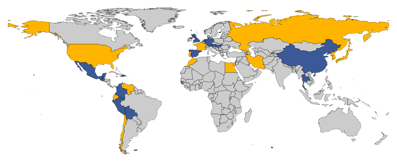
(a) 1816-1900

(b) 1900-1950

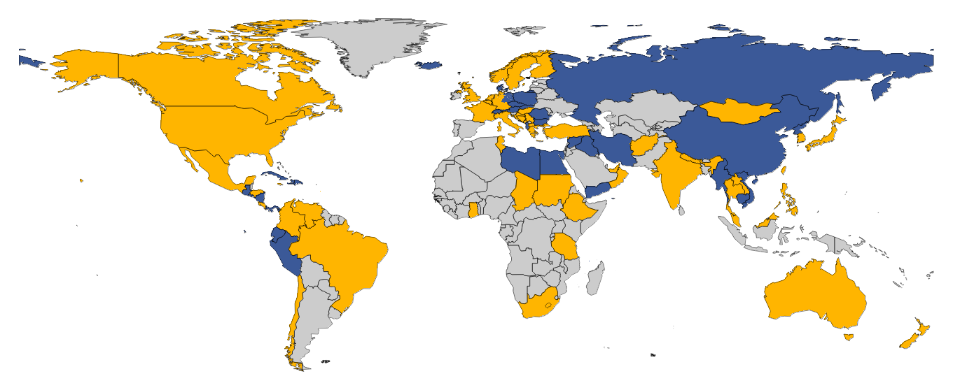
(c) 1950-1990

(d) 1990-2010

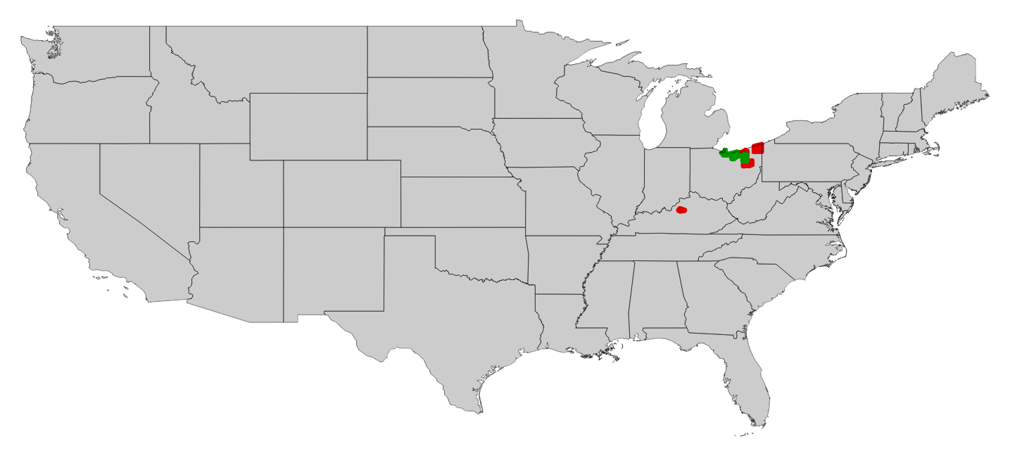
(e) Ohio Seed

(f) New York Seed

(g) California Seed

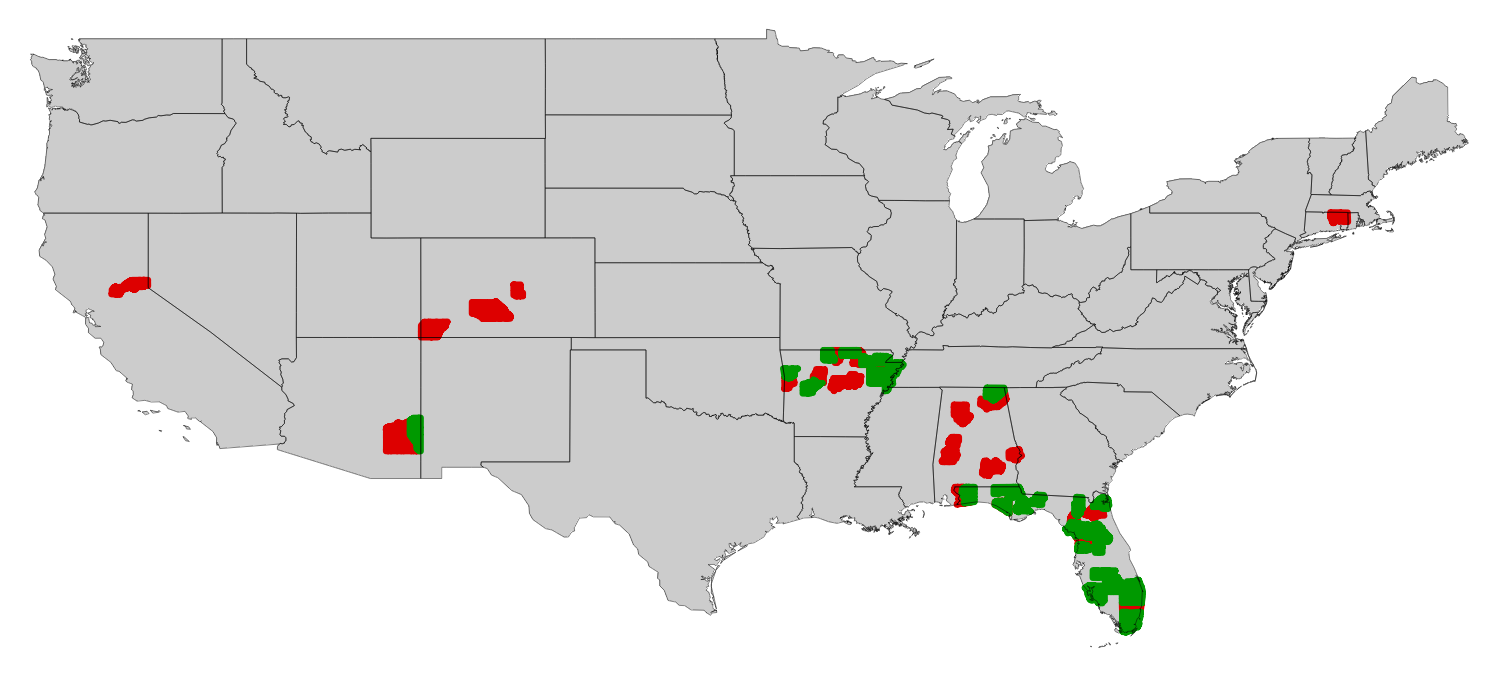
(h) Florida Seed

Figure 1: (a)-(d) Clusters found by LocBipartDC on the interstate dispute network, using the USA as the seed vertex. In each case, countries in the yellow cluster tend to enter conflicts with countries in the blue cluster and vice versa. (e)-(h) Clusters found by EvoCutDirected in the US migration network. There is a large net flow from the red counties to the green counties.

1 Introduction

Given an arbitrary vertex $u$ of a graph $G=(V,E)$ as input, a local graph clustering algorithm finds some low-conductance set $S\subset V$ containing $u$, while the algorithm runs in time proportional to the size of the target cluster and independent of the size of the graph $G$. Because of the increasing size of available datasets, which makes centralised computation too expensive, local graph clustering has become an important learning technique for analysing a number of large-scale graphs and has been applied to solve many other learning and combinatorial optimisation problems [1, 5, 11, 16, 25, 29, 30, 32].

1.1 Our Contribution

We study local graph clustering for learning the structure of clusters that are defined by their inter-connections, and present two local algorithms to achieve this objective in both undirected graphs and directed ones.

Our first result is a local algorithm for finding densely connected clusters in an undirected graph $G=(V,E)$: given any seed vertex $u$, our algorithm is designed to find two clusters $L,R$ around $u$, which are densely connected to each other and are loosely connected to $V\setminus(L\cup R)$. The design of our algorithm is based on a new reduction that allows us to relate the connections between $L,R$ and $V\setminus(L\cup R)$ to a single cluster in the resulting graph $H$, and a generalised analysis of Pagerank-based algorithms for local graph clustering. The significance of our designed algorithm is demonstrated by our experimental results on the Interstate Dispute Network from 1816 to 2010. By connecting two vertices (countries) with an undirected edge weighted according to the severity of their military disputes and using the USA as the seed vertex, our algorithm recovers two groups of countries that tend to have conflicts with each other, and shows how the two groups evolve over time. In particular, as shown in Figures 1(a)-(d), our algorithm not only identifies the changing roles of Russia, Japan, and eastern Europe in line with 20th century geopolitics, but also the reunification of east and west Germany around 1990.

We further study densely connected clusters in a directed graph (digraph). Specifically, given any vertex $u$ in a digraph $G=(V,E)$ as input, our second local algorithm outputs two disjoint vertex sets $L$ and $R$, such that (i) there are many edges from $L$ to $R$, and (ii) $L\cup R$ is loosely connected to $V\setminus(L\cup R)$. The design of our algorithm is based on the following two techniques: (1) a new reduction that allows us to relate the edge weight from $L$ to $R$, as well as the edge connections between $L\cup R$ and $V\setminus(L\cup R)$, to a single vertex set in the resulting undirected graph $H$; (2) a refined analysis of the ESP-based algorithm for local graph clustering. We show that our algorithm is able to recover local densely connected clusters in the US migration dataset, in which two vertex sets $L,R$ defined as above could represent a higher-order migration trend. In particular, as shown in Figures 1(e)–(h), by using different counties as starting vertices, our algorithm uncovers refined and more localised migration patterns than the previous work on the same dataset [10]. To the best of our knowledge, our work represents the first local clustering algorithm that achieves a similar goal.

1.2 Related Work

Li and Peng [15] study the same problem for undirected graphs, and present a random walk based algorithm. Andersen [1] studies a similar problem for undirected graphs under a different objective function, and our algorithm’s runtime significantly improves the one in [1]. There is some recent work on local clustering for hypergraphs [25], and algorithms for finding higher-order structures of graphs based on network motifs both centrally [7, 8] and locally [30]. These algorithms are designed to find different types of clusters, and cannot be directly compared with ours. Our problem is related to the problem of finding clusters in disassortative networks [22, 23, 31], although the existing techniques are based on semi-supervised, global methods while ours is unsupervised and local. There are also recent studies which find clusters with a specific structure in the centralised setting [10, 14]. Our current work shows that such clusters can be learned locally via our presented new techniques.

2 Preliminaries

Notation.

For any undirected and unweighted graph $G=(V_{G},E_{G})$ with $n$ vertices and $m$ edges, the degree of any vertex $v$ is denoted by $\deg_{G}(v)$, and the set of neighbours of $v$ is $N_{G}(v)$. For any $S\subseteq V$, its volume is $\mathrm{vol}_{G}(S)\triangleq\sum_{v\in S}\deg(v)$, its boundary is $\partial_{G}(S)\triangleq\{(u,v)\in E:u\in S~{}\mbox{and}~{}v\not\in S\}$, and its conductance is

$$\Phi_{G}(S)\triangleq\frac{|\partial_{G}(S)|}{\min\{\mathrm{vol}_{G}(S),\mathrm{vol}_{G}(V\setminus S)\}}.$$

For disjoint $S_{1},S_{2}\subset V_{G}$, $e(S_{1},S_{2})$ is the number of edges between $S_{1}$ and $S_{2}$. When $G=(V_{G},E_{G})$ is a digraph, for any $u\in V_{G}$ we use $\deg_{\mathrm{out}}(u)$ and $\deg_{\mathrm{in}}(u)$ to express the number of edges with $u$ as the tail or the head, respectively. For any $S\subset V_{G}$, we define $\mathrm{vol}_{\mathrm{out}}(S)=\sum_{u\in S}\deg_{\mathrm{out}}(u)$, and $\mathrm{vol}_{\mathrm{in}}(S)=\sum_{u\in S}\deg_{\mathrm{in}}(u)$.

For undirected graphs, we use $D_{G}$ to denote the $n\times n$ diagonal matrix with $(D_{G})_{v,v}=\deg_{G}(v)$ for any vertex $v\in V$, and we use $A_{G}$ to represent the adjacency matrix of $G$ defined by $(A_{G})_{u,v}=1$ if $\{u,v\}\in E_{G}$, and $(A_{G})_{u,v}=0$ otherwise. The lazy random walk matrix of $G$ is $W_{G}=(1/2)\cdot(I+D^{-1}_{G}A_{G})$. For any set $S\subset V_{G}$, $\chi_{S}$ is the indicator vector of $S$, i.e., $\chi_{S}(v)=1$ if $v\in S$, and $\chi_{S}(v)=0$ otherwise. If the set consists of a single vertex $v$, we write $\chi_{v}$ instead of $\chi_{\{v\}}$. Sometimes we drop the subscript $G$ when the underlying graph is clear from the context. For any vectors $x,y\in\mathbb{R}^{n}$, we write $x\preceq y$ if it holds for any $v$ that $x(v)\leq y(v)$. For any operators $f,g:\mathbb{R}^{n}\rightarrow\mathbb{R}^{n}$, we define $f\circ g:\mathbb{R}^{n}\rightarrow\mathbb{R}^{n}$ by $f\circ g(v)\triangleq f(g(v))$ for any $v$. For any vector $p$, we define the support of $p$ to be $\mathrm{supp}(p)=\{u:p(u)\neq 0\}$. The sweep sets of $p$ are defined by (1) ordering all the vertices such that

$$\frac{p(v_{1})}{\deg(v_{1})}\geq\frac{p(v_{2})}{\deg(v_{2})}\geq\ldots\geq\frac{p(v_{n})}{\deg(v_{n})},$$

and (2) constructing $S_{j}^{p}=\{v_{1},\ldots,v_{j}\}$ for $1\leq j\leq n$. Throughout this paper, we will consider vectors to be row vectors, so the random walk update step for a distribution $p$ is written as $pW$. For ease of presentation we consider only unweighted graphs; however, our analysis can be easily generalised to the weighted case. The omitted proofs can be found in the Appendix.

Pagerank.

Given an underlying graph $G$ with the lazy random walk matrix $W$, the personalised Pagerank vector $\mathrm{pr}(\alpha,s)$ is defined to be the unique solution of the equation

$$\mathrm{pr}(\alpha,s)=\alpha s+(1-\alpha)\mathrm{pr}(\alpha,s)W,$$ (1)

where $s\in\mathbb{R}^{n}_{\geq 0}$ is a starting vector and $\alpha\in(0,1]$ is called the teleport probability. Andersen et al. [4] show that the personalised Pagerank vector can be written as $\mathrm{pr}(\alpha,s)=\alpha\sum_{t=0}^{\infty}(1-\alpha)^{t}sW^{t}.$ Therefore, we could study $\mathrm{pr}(\alpha,s)$ through the following random process: pick some integer $t\in\mathbb{Z}_{\geq 0}$ with probability $\alpha(1-\alpha)^{t}$, and perform a $t$-step lazy random walk, where the starting vertex of the random walk is picked according to $s$. Then, $\mathrm{pr}(\alpha,s)$ describes the probability of reaching each vertex in this process.

Computing an exact Pagerank vector $\mathrm{pr}(\alpha,\chi_{v})$ is equivalent to computing the stationary distribution of a Markov chain on the vertex set $V$ which has a time complexity of $\Omega(n)$. However, since the probability mass of a personalised Pagerank vector is concentrated around some starting vertex, it is possible to compute a good approximation of the Pagerank vector in a local way. Andersen et al. [4] introduced the approximate Pagerank, which will be used in our analysis.

Definition 1.

A vector $p=\mathrm{apr}(\alpha,s,r)$ is an approximate Pagerank vector if $p+\mathrm{pr}(\alpha,r)=\mathrm{pr}(\alpha,s)$. The vector $r$ is called the residual vector.

The evolving set process.

The evolving set process (ESP) is a Markov chain whose states are sets of vertices $S_{i}\subseteq V$. Given a state $S_{i}$, the next state $S_{i+1}$ is determined by the following process: (1) choose $t\in[0,1]$ uniformly at random; (2) let $S_{i+1}=\{v\in V|\chi_{v}W\chi_{S_{i}}^{\intercal}\geq t\}$. The volume-biased ESP is a variant used to ensure that the Markov chain absorbs in the state $V$ rather than $\emptyset$. Andersen and Peres [2] gave a local algorithm for undirected graph clustering using the volume-biased ESP. In particular, they gave an algorithm $\texttt{GenerateSample}(u,T)$ which samples the $T$-th element from the volume-biased ESP with $S_{0}=\{u\}$.

3 The Algorithm for Undirected Graphs

Now we present a local algorithm for finding two clusters in an undirected graph with a dense cut between them. To formalise this notion, for any undirected graph $G=(V,E)$ and disjoint $L,R\subset V$, we follow Trevisan [27] and define the bipartiteness ratio

$$\beta(L,R)\triangleq 1-\frac{2e(L,R)}{\mathrm{vol}(L\cup R)}.$$

Notice that a low $\beta(L,R)$ value means that there is a dense cut between $L$ and $R$, and there is a sparse cut between $L\cup R$ and $V\setminus(L\cup R)$. In particular, $\beta(L,R)=0$ implies that $(L,R)$ forms a bipartite and connected component of $G$. We will describe a local algorithm for finding almost-bipartite sets $L$ and $R$ with a low value of $\beta(L,R)$.

3.1 The Reduction by Double Cover

The design of most local algorithms for finding a target set $S\subset V$ of low conductance is based on analysing the behaviour of random walks starting from vertices in $S$. In particular, when the conductance $\Phi_{G}(S)$ is low, a random walk starting from most vertices in $S$ will leave $S$ with low probability. However, for our setting, the target is a pair of sets $L,R$ with many connections between them. As such, a random walk starting in either $L$ or $R$ is very likely to leave the starting set. To address this, we introduce a novel technique based on the double cover of $G$ to reduce the problem of finding two sets of high conductance to the problem of finding one of low conductance.

Formally, for any undirected graph $G=(V_{G},E_{G})$, its double cover is the bipartite graph $H=(V_{H},E_{H})$ defined as follows: (1) every vertex $v\in V_{G}$ has two corresponding vertices $v_{1},v_{2}\in V_{H}$; (2) for every edge $\{u,v\}\in E_{G}$, there are edges $\{u_{1},v_{2}\}$ and $\{u_{2},v_{1}\}$ in $E_{H}$. See Figure 2 for an illustration.

Figure 2: An example of the construction of the double cover.

Now we present a tight connection between the value of $\beta(L,R)$ for any disjoint sets $L,R\subset V_{G}$ and the conductance of a single set in the double cover of $G$. To this end, for any $S\subset V_{G}$, we define $S_{1}\subset V_{H}$ and $S_{2}\subset V_{H}$ by $S_{1}\triangleq\{v_{1}~{}|~{}v\in S\}$ and $S_{2}\triangleq\{v_{2}~{}|~{}v\in S\}$. We formalise the connection in the following lemma.

Lemma 1.

Let $G$ be an undirected graph, $S\subset V$ with partitioning $(L,R)$, and $H$ be the double cover of $G$. Then, it holds that $\Phi_{H}(L_{1}\cup R_{2})=\beta_{G}(L,R)$.

Next we look at the other direction of this correspondence. Specifically, given any $S\subset V_{H}$ in the double cover of a graph $G$, we would like to find two disjoint sets $L\subset V_{G}$ and $R\subset V_{G}$ such that $\beta_{G}(L,R)=\Phi_{H}(S)$. However, such a connection does not hold in general. To overcome this, we restrict our attention to those subsets of $V_{H}$ which can be unambiguously interpreted as two disjoint sets in $V_{G}$.

Definition 2.

We call $S\subset V_{H}$ simple if $|\{v_{1},v_{2}\}\cap S|\leq 1$ holds for all $v\in V_{G}$.

Lemma 2.

For any simple set $S\subset V_{H}$, let $L=\{u:u_{1}\in S\}$ and $R=\{u:u_{2}\in S\}$. Then, $\beta_{G}(L,R)=\Phi_{H}(S).$

3.2 Design of the Algorithm

So far we have shown that the problem of finding densely connected sets $L,R\subset V_{G}$ can be reduced to finding $S\subset V_{H}$ of low conductance in the double cover $H$, and this reduction raises the natural question of whether existing local algorithms can be directly employed to find $L$ and $R$ in $G$. However, this is not the case: even though a set $S\subset V_{H}$ returned by most local algorithms is guaranteed to have low conductance, vertices of $G$ could be included in $S$ twice, and as such $S$ will not necessarily give us disjoint sets $L,R\subset V_{G}$ with low value of $\beta(L,R)$. See Figure 3 for an illustration.

Figure 3: The indicated vertex set $S\subset V_{H}$ has low conductance. However, since $S$ contains many pairs of vertices which correspond to the same vertex in $G$, $S$ gives us little information for finding disjoint $L,R\subset V_{G}$ with a low $\beta(L,R)$ value.

The simplify operator.

To take the example shown in Figure 3 into account, our objective is to design a local algorithm for finding some set $S\subset V_{H}$ of low conductance which is also simple. To ensure this, we introduce the simplify operator, and analyse its properties.

Definition 3 (Simplify operator).

Let $H$ be the double cover of $G$, where the two corresponding vertices of any $u\in V_{G}$ are defined as $u_{1},u_{2}\in V_{H}$. Then, for any $p\in\mathbb{R}^{2n}_{\geq 0}$, the simplify operator is a function $\sigma:\mathbb{R}^{2n}_{\geq 0}\rightarrow\mathbb{R}^{2n}_{\geq 0}$ defined by

$$(\sigma\circ p)(u_{1}) \triangleq\max(0,p(u_{1})-p(u_{2})),$$

$$(\sigma\circ p)(u_{2}) \triangleq\max(0,p(u_{2})-p(u_{1}))$$

for every $u\in V_{G}$.

Notice that, for any vector $p$ and any $u\in V_{G}$, at most one of $u_{1}$ and $u_{2}$ is in the support of $\sigma\circ p$; hence, the support of $\sigma\circ p$ is always simple. To explain the meaning of $\sigma$, for a vector $p$ one could view $p(u_{1})$ as our “confidence” that $u\in L$, and $p(u_{2})$ as our “confidence” that $u\in R$. Hence, when $p(u_{1})\approx p(u_{2})$, both $(\sigma\circ p)(u_{1})$ and $(\sigma\circ p)(u_{2})$ are small which captures the fact that we would not prefer to include $u$ in either $L$ or $R$. On the other hand, when $p(u_{1})\gg p(u_{2})$, we have $(\sigma\circ p)(u_{1})\approx p(u_{1})$, which captures our confidence that $u$ should belong to $L$. The following lemma summaries some key properties of $\sigma$.

Lemma 3.

The following holds for the $\sigma$-operator:

• $\sigma\circ(c\cdot p)=c\cdot(\sigma\circ p)$ for $p\in\mathbb{R}_{\geq 0}^{2n}$ and any $c\in\mathbb{R}_{\geq 0}$;

• $\sigma\circ(a+b)\preceq\sigma\circ a+\sigma\circ b$ for $a,b\in\mathbb{R}_{\geq 0}^{2n}$;

• $\sigma\circ(pW)\preceq(\sigma\circ p)W$ for $p\in\mathbb{R}_{\geq 0}^{2n}$.

While these three properties will all be used in our analysis, the third is of particular importance: it implies that, if $p$ is the probability distribution of a random walk in $H$, applying $\sigma$ before taking a one-step random walk would never result in lower probability mass than applying $\sigma$ after taking a one-step random walk. This means that no probability mass would be lost when the $\sigma$-operator is applied between every step of a random walk, in comparison with applying $\sigma$ at the end of an entire random walk process.

Description of the algorithm.

Our proposed algorithm is conceptually simple: every vertex $u$ of the input graph $G$ maintains two copies $u_{1},u_{2}$ of itself, and these two “virtual” vertices are used to simulate $u$’s corresponding vertices in the double cover $H$ of $G$. Then, as the neighbours of $u_{1}$ and $u_{2}$ in $H$ are entirely determined by $u$’s neighbours in $G$ and can be constructed locally, a random walk process in $H$ will be simulated in $G$. This will allow us to apply a local algorithm similar to the one by Anderson et al. [4] on this “virtual” graph $H$. Finally, since all the required information about $u_{1},u_{2}\in V_{H}$ is maintained by $u\in V_{G}$, the $\sigma$-operator will be applied locally.

The formal description of our algorithm is given in Algorithm 1, which invokes Algorithm 2 as the key component to compute $\mathrm{apr}_{H}(\alpha,\chi_{u_{1}},r)$. Specifically, Algorithm 2 maintains, for every vertex $u\in G$, tuples $(p(u_{1}),p(u_{2}))$ and $(r(u_{1}),r(u_{2}))$ to keep track of the values of $p$ and $r$ in $G$’s double cover. For a given vertex $u$, the entries in these tuples are expressed by $p_{1}(u),p_{2}(u),r_{1}(u),$ and $r_{2}(u)$ respectively. Every dcpush operation (Algorithm 3) preserves the invariant $p+\mathrm{pr}_{H}(\alpha,r)=\mathrm{pr}_{H}(\alpha,\chi_{v_{1}}),$ which ensures that the final output of Algorithm 2 is an approximate Pagerank vector. We remark that, although the presentation of the ApproximatePagerankDC procedure is similar to the one in Andersen et al. [4], in our dcpush procedure the update of the residual vector $r$ is slightly more involved: specifically, for every vertex $u\in V_{G}$, both $r_{1}(u)$ and $r_{2}(u)$ are needed in order to update $r_{1}(u)$ (or $r_{2}(u)$). That is one of the reasons that the performance of the algorithm in Andersen et al. [4] cannot be directly applied for our algorithm, and a more technical analysis, some of which is parallel to theirs, is needed in order to analyse the correctness and performance of our algorithm.

  Input: A graph $G$, starting vertex $u$, target volume $\gamma$, and target bipartiteness $\beta$

  Output: Two disjoint sets $L$ and $R$

1  Set $\alpha=\frac{\beta^{2}}{378}$, and $\epsilon=\frac{1}{20\gamma}$

Compute $p^{\prime}=\texttt{ApproximatePagerankDC}(u,\alpha,\epsilon)$

  Compute $p=\sigma\circ p^{\prime}$

  for $j\in[1,|\mathrm{supp}(p)|]$ do

     if $\Phi(S_{j}^{p})\leq\beta$ then

2        Set $L=\{u:u_{1}\in S_{j}^{p}\}$, and $R=\{u:u_{2}\in S_{j}^{p}\}$

return $(L,R)$

     end if

  end for

Algorithm 1 LocBipartDC

  Input: Starting vertex $v$, parameters $\alpha$ and $\epsilon$

  Output: Approximate Pagerank vector $\mathrm{apr}_{H}(\alpha,\chi_{v_{1}},r)$

  Set $p_{1}=p_{2}=r_{2}=\mathbf{0}$; set $r_{1}=\chi_{v}$

  while $\max_{(u,i)\in V\times\{1,2\}}\frac{r_{i}(u)}{\deg(u)}\geq\epsilon$ do

     Choose any $u$ and $i\in\{1,2\}$ such that $\frac{r_{i}(u)}{\deg(u)}\geq\epsilon$

     $(p_{1},p_{2},r_{1},r_{2})=\texttt{dcpush}(\alpha,(u,i),p_{1},p_{2},r_{1},r_{2})$

1  end while

return $p=\left[p_{1},p_{2}\right]$

Algorithm 2 ApproximatePagerankDC

  Input: $\alpha,(u,i),p_{1},p_{2},r_{1},r_{2}$

  Output: $(p^{\prime}_{1},p^{\prime}_{2},r^{\prime}_{1},r^{\prime}_{2})$

  Set $(p_{1}^{\prime},p_{2}^{\prime},r_{1}^{\prime},r_{2}^{\prime})=(p_{1},p_{2},r_{1},r_{2})$

1  Set $p^{\prime}_{i}(u)=p_{i}(u)+\alpha r_{i}(u)$; $r^{\prime}_{i}(u)=(1-\alpha)\frac{r_{i}(u)}{2}$

  for $v\in N_{G}(u)$ do

     Set $r^{\prime}_{3-i}(v)=r_{3-i}(v)+(1-\alpha)\frac{r_{i}(u)}{2\deg(u)}$

2  end for

return $(p^{\prime}_{1},p^{\prime}_{2},r^{\prime}_{1},r^{\prime}_{2})$

Algorithm 3 dcpush

3.3 Analysis of the Algorithm

To prove the correctness of our algorithm, we will show two complementary facts which we state informally here:

1. If there is a simple set $S\subset V_{H}$ with low conductance, then for most $u_{1}\in S$, the simplified approximate Pagerank vector $p=\sigma\circ\mathrm{apr}(\alpha,\chi_{u_{1}},r)$ will have a lot of probability mass on a small set of vertices.

2. If $p=\sigma\circ\mathrm{apr}(\alpha,\chi_{u_{1}},r)$ contains a lot of probability mass on some small set of vertices, then there is a sweep set of $p$ with low conductance.

As we have shown in Section 3.1, there is a direct correspondence between almost-bipartite sets in $G$, and low-conductance and simple sets in $H$. This means that the two facts above are exactly what we need to prove that Algorithm 1 can find densely connected sets in $G$.

We will first show in Lemma 4 how the $\sigma$-operator affects some standard mixing properties of Pagerank vectors in order to establish the first fact promised above. This lemma relies on the fact that $S\subset V_{G}$ corresponds to a simple set in $V_{H}$. This allows us to apply the $\sigma$-operator to the approximate Pagerank vector $\mathrm{apr}_{H}(\alpha,\chi_{u_{1}},r)$ while preserving a large probability mass on the target set.

Lemma 4.

For any set $S\subset V_{G}$ with partitioning $(L,R)$ and any constant $\alpha\in[0,1]$, there is a subset $S_{\alpha}\subseteq S$ with $\mathrm{vol}(S_{\alpha})\geq\mathrm{vol}(S)/2$ such that, for any vertex $v\in S_{\alpha}$, the simplified approximate Pagerank on the double cover $p=\sigma\circ\left(\mathrm{apr}_{H}(\alpha,\chi_{v_{1}},r)\right)$ satisfies

$$p(L_{1}\cup R_{2})\geq 1-\frac{2\beta(L,R)}{\alpha}-2\mathrm{vol}(S)\max_{u\in V}\frac{r(u)}{\deg(u)}.$$

To prove the second fact, we show as an intermediate lemma that the value of $p(u_{1})$ can be bounded with respect to its value after taking a step of the random walk: $pW(u_{1})$.

Lemma 5.

Let $G$ be a graph with double cover $H$, and $\mathrm{apr}(\alpha,s,r)$ be the approximate Pagerank vector defined with respect to $H$. Then, $p=\sigma\circ\left(\mathrm{apr}(\alpha,s,r)\right)$ satisfies that $p(u_{1})\leq\alpha\left(s(u_{1})+r(u_{2})\right)+(1-\alpha)(pW)(u_{1})$, and $p(u_{2})\leq\alpha\left(s(u_{2})+r(u_{1})\right)+(1-\alpha)(pW)(u_{2})$ for any $u\in V_{G}$.

Notice that applying the $\sigma$-operator for any vertex $u_{1}$ introduces a new dependency on the value of the residual vector $r$ at $u_{2}$. This subtle observation demonstrates the additional complexity introduced by the $\sigma$-operator when compared with previous analysis of Pagerank-based local algorithms [4]. Taking account of the $\sigma$-operator, we further analyse the Lovász-Simonovits curve defined by $p$, which is a common technique in the analysis of random walks on graphs [17]: we show that if there is a set $S$ with a large value of $p(S)$, there must be a sweep set $S_{j}^{p}$ with small conductance.

Lemma 6.

Let $G$ be a graph with double cover $H$, and let $p=\sigma\circ\left(\mathrm{apr}_{H}(\alpha,s,r)\right)$ such that $\max_{u\in V_{H}}\frac{r(u)}{d(u)}\leq\epsilon$. If there is a set of vertices $S\subset V_{H}$ and a constant $\delta$ such that $p(S)-\frac{\mathrm{vol}(S)}{\mathrm{vol}(V_{H})}\geq\delta$, then there is some $j\in[1,\left\lvert\mathrm{supp}(p)\right\rvert]$ such that $\Phi_{H}(S_{j}^{p})<6\sqrt{(1+\epsilon\mathrm{vol}(S))\alpha\ln(\frac{4}{\delta})\big{/}\delta}$.

We have now shown the two facts promised at the beginning of this subsection. Putting these together, if there is a simple set $S\subset V_{H}$ with low conductance then we can find a sweep set of $\sigma\circ\mathrm{apr}(\alpha,s,r)$ with low conductance. By the reduction from almost-bipartite sets in $G$ to low-conductance simple sets in $H$ our target set corresponds to a simple set $S\subset V_{H}$ which leads to Algorithm 1 for finding almost-bipartite sets. Our result is summarised as follows.

Theorem 1.

Let $G$ be an $n$-vertex undirected graph, and $L,R\subset V_{G}$ be disjoint sets such that $\beta(L,R)\leq\beta$ and $\mathrm{vol}(L\cup R)\leq\gamma$. Then, there is a set $C\subseteq L\cup R$ with $\mathrm{vol}(C)\geq\mathrm{vol}(L\cup R)/2$ such that, for any $v\in C$, $\texttt{LocBipartDC}\left(G,v,\gamma,\sqrt{7560\beta}\right)$ returns $(L^{\prime},R^{\prime})$ with $\beta(L^{\prime},R^{\prime})=O\!\left(\sqrt{\beta}\right)$ and ${\mathrm{vol}(L^{\prime}\cup R^{\prime})}=O\!\left(\beta^{-1}\gamma\right)$. Moreover, the algorithm has running time $O\!\left(\beta^{-1}\gamma\log n\right)$.

The quadratic approximation guarantee in Theorem 1 matches the state-of-the-art local algorithm for finding a single set with low conductance [5]. Furthermore, our result presents a significant improvement over the previous state-of-the-art by Li and Peng [15], whose design is based on an entirely different technique than ours. For any $\epsilon\in[0,1/2]$, their algorithm runs in time $O\!\left(\epsilon^{2}\beta^{-2}\gamma^{1+\epsilon}\log^{3}\gamma\right)$ and returns a set with volume $O\!\left(\gamma^{1+\epsilon}\right)$ and bipartiteness ratio $O\!\left(\sqrt{\beta/\epsilon}\right)$. In particular, their algorithm requires much higher time complexity in order to guarantee the same bipartiteness ratio $O\left(\sqrt{\beta}\right)$.

4 The Algorithm for Digraphs

We now turn our attention to local algorithms for finding densely-connected clusters in digraphs. In comparison with undirected graphs, we are interested in finding disjoint $L,R\subset V$ of some digraph $G=(V,E)$ such that most of the edges adjacent to $L\cup R$ are from $L$ to $R$. To formalise this, we define the flow ratio from $L$ to $R$ as

$$F(L,R)\triangleq 1-\frac{2e(L,R)}{\mathrm{vol}_{\mathrm{out}}(L)+\mathrm{vol}_{\mathrm{in}}(R)},$$

where $e(L,R)$ is the number of directed edges from $L$ to $R$. Notice that we take not only edge densities but also edge directions into account: a low $F(L,R)$-value tells us that almost all edges with their tail in $L$ have their head in $R$, and conversely almost all edges with their head in $R$ have their tail in $L$. One could also see $F(L,R)$ as a generalisation of $\beta(L,R)$. In particular, if we view an undirected graph as a digraph by replacing each edge with two directed edges, then $\beta(L,R)=F(L,R)$. In this section, we will present a local algorithm for finding such vertex sets in a digraph, and analyse the algorithm’s performance.

4.1 The Reduction by Semi-Double Cover

Given a digraph $G=(V_{G},E_{G})$, we construct its semi-double cover $H=(V_{H},E_{H})$ as follows: (1) every vertex $v\in V_{G}$ has two corresponding vertices $v_{1},v_{2}\in V_{H}$; (2) for every edge $(u,v)\in E_{G}$, we add the edge $\{u_{1},v_{2}\}$ in $E_{H}$, see Figure 4 for illustration. It is worth comparing this reduction with the one for undirected graphs:

• For undirected graphs, we apply the standard double cover and every undirected edge in $G$ corresponds to two edges in the double cover $H$;

• For digraphs, every directed edge in $G$ corresponds to one undirected edge in $H$. This asymmetry would allow us to “recover” the direction of any edge in $G$.

Figure 4: An example of a digraph and its semi-double cover.

We follow the use of $S_{1},S_{2}$ from Section 3: for any $S\subset V_{G}$, we define $S_{1}\subset V_{H}$ and $S_{2}\subset V_{H}$ by $S_{1}\triangleq\{v_{1}~{}|~{}v\in S\}$ and $S_{2}\triangleq\{v_{2}~{}|~{}v\in S\}$. The lemma below shows the connection between the value of $F_{G}(L,R)$ for any $L,R$ and $\Phi_{H}(L_{1}\cup R_{2})$.

Lemma 7.

Let $G$ be a digraph with semi-double cover $H$. Then, it holds for any $L,R\subset V_{G}$ that $F_{G}(L,R)=\Phi_{H}(L_{1}\cup R_{2})$. Similarly, for any simple set $S\subset V_{H}$, let $L=\{u:u_{1}\in S\}$ and $R=\{u:u_{2}\in S\}$. Then, it holds that $F_{G}(L,R)=\Phi_{H}(S)$.

4.2 Design and Analysis of the Algorithm

Our presented algorithm is a modification of the algorithm by Andersen and Peres [2]. Given a digraph $G$ as input, our algorithm simulates the volume-biased ESP on $G$’s semi-double cover $H$. Notice that the graph $H$ can be constructed locally in the same way as the local construction of the double cover. However, as the output set $S$ of an ESP-based algorithm is not necessarily simple, our algorithm only returns vertices $u\in V_{G}$ in which exactly one of $u_{1}$ and $u_{2}$ are included in $S$. The key procedure for our algorithm is given in Algorithm 4, in which the GenerateSample procedure is the one described at the end of Section 2.

  Input: Starting vertex $u$, $i\in\{1,2\}$, target flow ratio $\phi$

  Output: A pair of sets $L,R\subset V_{G}$

  Set $T=\lfloor(100\phi^{\frac{2}{3}})^{-1}\rfloor$.

  Compute $S=\texttt{GenerateSample}_{H}(u_{i},T)$

  Let $L=\{u\in V_{G}:u_{1}\in S$ and $u_{2}\not\in S\}$

1  Let $R=\{u\in V_{G}:u_{2}\in S$ and $u_{1}\not\in S\}$

return $L$ and $R$

Algorithm 4 EvoCutDirected (ECD)

Notice that in our constructed graph $H$, $\Phi(L_{1}\cup R_{2})\leq\phi$ does not imply that $\Phi(L_{2}\cup R_{1})\leq\phi$. Due to this asymmetry, Algorithm 4 takes a parameter $i\in\{1,2\}$ to indicate whether the starting vertex is in $L$ or $R$. If it is not known whether $u$ is in $L$ or $R$, two copies can be run in parallel, one with $i=1$ and the other with $i=2$. Once one of them terminates with the performance guaranteed in Theorem 2, the other can be terminated. Hence, we can always assume that it is known whether the starting vertex $u$ is in $L$ or $R$.

Now we sketch the analysis of the algorithm. Notice that, since the evolving set process gives us an arbitrary set on the semi-double cover, in Algorithm 4 we convert this into a simple set by removing any vertices $u$ where $u_{1}\in S$ and $u_{2}\in S$. The following definition allows us to discuss sets which are close to being simple.

Definition 4 ($\epsilon$-simple set).

For any set $S\subset V_{H}$, let $P=\{u_{1},u_{2}:u\in V_{G},u_{1}\in S~{}\mbox{and}~{}u_{2}\in S\}$. We call set $S$ $\epsilon$-simple if it holds that $\frac{\mathrm{vol}(P)}{\mathrm{vol}(S)}\leq\epsilon.$

The notion of $\epsilon$-simple sets measures the ratio of vertices in which both $u_{1}$ and $u_{2}$ are in $S$. In particular, any simple set defined in Definition 2 is $0$-simple. We show that, for any $\epsilon$-simple set $S\subset V_{H}$, one can construct a simple set $S^{\prime}$ such that $\Phi(S^{\prime})\leq\frac{1}{1-\epsilon}\cdot\left(\Phi(S)+\epsilon\right)$. Therefore, in order to guarantee that $\Phi(S^{\prime})$ is small, we need to construct $S$ such that $\Phi(S)$ is small and $S$ is $\epsilon$-simple for small $\epsilon$. Because of this, our presented algorithm uses a lower value of $T$ than the algorithm in Andersen and Peres [2]; this allows us to better control $\mathrm{vol}(S)$ at the cost of a slightly worse approximation guarantee. Our algorithm’s performance is summarised in Theorem 2.

Theorem 2.

Let $G$ be an $n$-vertex digraph, and $L,R\subset V_{G}$ be disjoint sets such that $F(L,R)\leq\phi$ and $\mathrm{vol}(L\cup R)\leq\gamma$. There is a set $C\subseteq L\cup R$ with $\mathrm{vol}(C)\geq\mathrm{vol}(L\cup R)/2$ such that, for any $v\in C$ and some $i\in\{1,2\}$, $\texttt{EvoCutDirected}(G,v,i,\phi)$ returns $(L^{\prime},R^{\prime})$ such that $F(L^{\prime},R^{\prime})=O\!\left(\phi^{\frac{1}{3}}\log^{\frac{1}{2}}n\right)$ and ${\mathrm{vol}(L^{\prime}\cup R^{\prime})}=O\left((1-\phi^{\frac{1}{3}})^{-1}\gamma\right)$. Moreover, the algorithm has running time $O\!\left(\phi^{-\frac{1}{2}}\gamma\log^{\frac{3}{2}}n\right)$.

To the best of our knowledge, this is the first local algorithm for digraphs that approximates a pair of densely connected clusters, and demonstrates that finding such a pair appears to be much easier than finding a low-conductance set in a digraph; in particular, existing local algorithms for finding a low-conductance set require the stationary distribution of the random walk in the digraph [3], the sublinear-time computation of which is unknown [9]. However, knowledge of the stationary distribution is not needed for our algorithm.

Further Discussion.

It is important to note that the semi-double cover construction is able to handle directed graphs which contain edges between two vertices $u$ and $v$ in both directions. In other words, the adjacency matrix of the digraph need not be skew-symmetric. This is an advantage of our approach over previous methods (e.g., [10]), and it would be a meaningful research direction to identify the benefit this gives our developed reduction.

It is also insightful to discuss why Algorithm 1 cannot be applied for digraphs, although the input digraph is translated into an undirected graph by our reduction. This is because, when translating a digraph into a bipartite undirected graph, the third property of the $\sigma$-operator in Lemma 3 no longer holds, since the existence of the edge $\{u_{1},v_{2}\}\in E_{H}$ does not necessarily imply that $\{u_{2},v_{1}\}\in E_{H}$. Indeed, Figure 5 gives a counterexample in which $\left(\sigma\circ(pW)\right)(u)\not\leq\left((\sigma\circ p)W\right)(u)$. This means that the typical analysis of a Pagerank vector with the Lovász-Simonovitz curve cannot be applied anymore. In our point of view, constructing some operator similar to our $\sigma$-operator and designing a Pagerank-based local algorithm for digraphs based on such an operator is a very interesting open question, and may help to close the gap in the approximation guarantee between the undirected and directed cases.

Figure 5: Consider the digraph and its semi-double cover above. Suppose $p(a_{1})=p(a_{2})=0.5$ and $p(b_{1})=p(b_{2})=0$. It is straightforward to check that $(\sigma\circ(pW))(b_{2})=0.25$ and $((\sigma\circ p)W)(b_{2})=0$.

In addition, we underline that one cannot apply the tighter analysis of the ESP process given by Andersen et al. [5] to our algorithm. The key to their analysis is an improved bound on the probability that a random walk escapes from the target cluster. In order to take advantage of this, they use a larger value of $T$ in the algorithm which relaxes the guarantee on the volume of the output set. Since our analysis relies on a very tight guarantee on the overlap of the output set with the target set, we cannot use their improvement in our setting.

5 Experiments

In this section we evaluate the performance of our proposed algorithms on both synthetic and real-world data sets. For undirected graphs, we compare the performance of our algorithm against the previous state-of-the-art [15], through the synthetic dataset with various parameters and apply the real-world dataset to demonstrate the significance of our algorithm. For directed graphs, we compare the performance of our algorithm with the state-of-the-art non-local algorithm since, to the best of our knowledge, our local algorithm for digraphs is the first such algorithm in the literature. All experiments were performed on a Lenovo Yoga 2 Pro with an Intel(R) Core(TM) i7-4510U CPU @ 2.00GHz processor and 8GB of RAM. Our code can be downloaded from https://github.com/pmacg/local-densely-connected-clusters.

5.1 Results for Undirected Graphs

5.1.1 Experiments on Synthetic Data

We first compare the performance of our algorithm, LocBipartDC, with the previous state-of-the-art given by Li & Peng [15], which we refer to as LP, on synthetic graphs generated from the stochastic block model (SBM). Specifically, we assume that the graph has $k=3$ clusters $\{C_{j}\}_{j=1}^{3}$, and the number of vertices in each cluster, denoted by $n_{1},n_{2}$ and $n_{3}$ respectively, satisfy $n_{1}=n_{2}=0.1n_{3}$. Moreover, any pair of vertices $u\in C_{i}$ and $v\in C_{j}$ is connected with probability $P_{i,j}$. We assume that $P_{1,1}=P_{2,2}=p_{1}$, $P_{3,3}=p_{2}$, $P_{1,2}=q_{1}$, and $P_{1,3}=P_{2,3}=q_{2}$. Throughout our experiments, we maintain the ratios $p_{2}=2p_{1}$ and $q_{2}=0.1p_{1}$, leaving the parameters $n_{1}$, $p_{1}$ and $q_{1}$ free. Notice that the different values of $q_{1}$ and $q_{2}$ guarantee that $C_{1}$ and $C_{2}$ are the ones optimising the $\beta$-value, which is why our proposed model is slightly more involved than the standard SBM.

We evaluate the quality of the output $(L,R)$ returned by each algorithm with respect to its $\beta$-value, the Adjusted Rand Index (ARI) [12], as well as the ratio of the misclassified vertices defined by $\frac{\left\lvert L\triangle C_{1}\right\rvert+\left\lvert R\triangle C_{2}\right\rvert}{\left\lvert L\cup C_{1}\right\rvert+\left\lvert R\cup C_{2}\right\rvert}$, where $A\triangle B$ is the symmetric difference between $A$ and $B$. All our reported results are the average performance of each algorithm over $10$ runs, in which a random vertex from $C_{1}\cup C_{2}$ is chosen as the starting vertex of the algorithm.

Setting the $\epsilon$ parameter in the LP algorithm.

The LP algorithm has an additional parameter over ours, which we refer to as $\epsilon_{LP}$. This parameter influences the runtime and performance of the algorithm and must be in the range $[0,1/2]$. In order to choose a fair value of $\epsilon_{LP}$ for comparison with our algorithm, we consider several values on graphs with a range of target volumes.

We generate graphs from the SBM such that $p_{1}=1/n_{1}$ and $q_{1}=100p_{1}$ and vary the size of the target set by varying $n_{1}$ between $100$ and $10,000$. For values of $\epsilon_{LP}$ in $\{0.01,0.02,0.1,0.5\}$, Figure 6(a) shows how the runtime of the LP algorithm compares to the LocBipartDC algorithm for a range of target volumes. In this experiment, the runtime of the LocBipartDC algorithm lies between the runtimes of the LP algorithm for $\epsilon_{LP}=0.01$ and $\epsilon_{LP}=0.02$. However, Figure 6(b) shows that the performance of the LP algorithm with $\epsilon_{LP}=0.01$ is significantly worse than the performance of the LocBipartDC algorithm and so for a fair comparison, we set $\epsilon_{LP}=0.02$ for the remainder of the experiments.

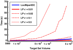
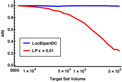
Figure 6: (a) A comparison of the runtimes of the LocBipartDC algorithm and the LP algorithm with various values of $\epsilon_{LP}$. (b) Setting $\epsilon_{LP}=0.01$ results in significantly worse performance than the LocBipartDC algorithm.

Comparison on the Synthetic Data.

Table 1: Full comparison between Algorithm 1 (LBDC) and the previous state-of-the-art [15] (LP). For clarity we report the target bipartiteness $\beta=\beta(C_{1},C_{2})$ and target volume $\gamma=\mathrm{vol}(C_{1}\cup C_{2})$ along with the SBM parameters.

Input graph parameters	Algo.	Runtime	$\beta$-value	ARI	Misclassified Ratio
$n_{1}=1,000$, $p_{1}=0.001$, $q_{1}=0.018$	LBDC	0.09	0.154	0.968	0.073
$\beta\approx 0.1$, $\gamma\approx 40,000$	LP	0.146	0.202	0.909	0.138
$n_{1}=10,000$, $p_{1}=0.0001$, $q_{1}=0.0018$	LBDC	0.992	0.215	0.940	0.145
$\beta\approx 0.1$, $\gamma\approx 400,000$	LP	1.327	0.297	0.857	0.256
$n_{1}=100,000$, $p_{1}=0.00001$, $q_{1}=0.00018$	LBDC	19.585	0.250	0.950	0.166
$\beta\approx 0.1$, $\gamma\approx 4,000,000$	LP	30.285	0.300	0.865	0.225
$n_{1}=1,000$, $p_{1}=0.004$, $q_{1}=0.012$	LBDC	1.249	0.506	0.503	0.763
$\beta\approx 0.4$, $\gamma\approx 40,000$	LP	1.329	0.597	0.445	0.785

We now compare the LocBipartDC and LP algorithms’ performance on graphs generated from the SBM with different values of $n_{1},p_{1}$ and $q_{1}$. As shown in Table 1, our algorithm not only runs faster, but also produces better clusters with respect to all three metrics. Secondly, since the clustering task becomes more challenging when the target clusters have higher $\beta$-value, we compare the algorithms’ performance on a sequence of instances with increasing value of $\beta$. Since $q_{1}/p_{1}=2(1-\beta)/\beta$, we simply fix the values of $n_{1},p_{1}$ as $n_{1}=1,000,p_{1}=0.001$, and generate graphs with increasing value of $q_{1}/p_{1}$; this gives us graphs with monotone values of $\beta$. As shown in Figure 7, our algorithms performance is always better than the previous stat-of-the-art.

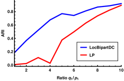
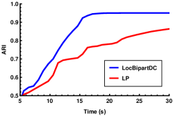
Figure 7: (a) The ARI of each algorithm when varying the target $\beta$-value. A larger $q_{1}/p_{1}$ ratio corresponds to a smaller $\beta$-value. (b) The ARI of each algorithm when bounding the runtime of the algorithm.

Thirdly, notice that both algorithms use some parameters to control the algorithm’s runtime and the output’s approximation ratio, which are naturally influenced by each other. To study this dependency, we generate graphs according to $n_{1}=100,000$, $p_{1}=0.000015$, and $q_{1}=0.00027$ which results in target sets with $\beta\approx 0.1$ and volume $\gamma\approx 6,000,000$. Figure 7(b) shows that, in comparison with the previous state-of-the-art, our algorithm takes much less time to produce output with the same ARI value.

5.1.2 Experiments on the Real-world Dataset

We demonstrate the significance of our algorithm on the Dyadic Militarised Interstate Disputes Dataset (v3.1) [19], which records every interstate dispute during 1816–2010, including the level of hostility resulting from the dispute and the number of casualties, and has been widely studied in the social and political sciences [18, 20] as well as the machine learning community [13, 21, 26]. For a given time period, we construct a graph from the data by representing each country with a vertex and adding an edge between each pair of countries weighted according to the severity of any military disputes between those countries. Specifically, if there’s a war between the two countries, the corresponding two vertices are connected by an edge with weight $30$; for any other dispute that is not part of an interstate war, the two corresponding vertices are connected by an edge with weight $1$. We always use the USA as the starting vertex of the algorithm, and our algorithm’s output, as visualised in Figure 1(a)-(d), can be well explained by geopolitics. The $\beta$-values of the pairs of clusters in Figures 1(a)-(d) are $0.361$, $0.356$, $0.170$ and $0.191$ respectively.

5.2 Results for Digraphs

Next we evaluate the performance of our algorithm for digraphs on synthetic and real-world datasets. Since there are no previous local digraph clustering algorithms that achieve similar objectives to ours, we compare the output of Algorithm 4 (ECD) with the state-of-the-art non-local algorithm proposed by Cucuringu et al. [10], and we refer this to as CLSZ in the following.

Synthetic Dataset.

We first look at the cyclic block model (CBM) described in Cucuringu et al. [10] with parameters $k$, $n$, $p$, $q$, and $\eta$. In this model, we generate a digraph with $k$ clusters $C_{1},\ldots,C_{k}$ of size $n$, and for $u,v\in C_{i}$, there is an edge between $u$ and $v$ with probability $p$ and the edge direction is chosen uniformly at random. For $u\in C_{i}$ and $v\in C_{i+1\mod k}$, there is an edge between $u$ and $v$ with probability $q$, and the edge is directed from $u$ to $v$ with probability $\eta$ and from $v$ to $u$ with probability $1-\eta$. Throughout our experiments, we fix $p=0.001$, $q=0.01$, and $\eta=0.9$.

Secondly, since the goal of our algorithm is to find local structure in a graph, we extend the cyclic block model with additional local clusters and refer to this model as CBM+. In addition to the parameters of the CBM, we introduce the parameters $n^{\prime},q^{\prime}_{1},q^{\prime}_{2}$, and $\eta^{\prime}$. In this model, the clusters $C_{1}$ to $C_{k}$ are generated as in the CBM, and there are two additional clusters $C_{k+1}$ and $C_{k+2}$ of size $n^{\prime}$. For $u,v\in C_{k+i}$ for $i\in\{1,2\}$, there is an edge between $u$ and $v$ with probability $p$ and for $u\in C_{k+1}$ and $v\in C_{k+2}$, there is an edge with probability $q^{\prime}_{1}$; the edge directions are chosen uniformly at random. For $u\in C_{k+1}\cup C_{k+2}$ and $v\in C_{1}$, there is an edge with probability $q^{\prime}_{2}$. If $u\in C_{k+1}$, the orientation is from $v$ to $u$ with probability $\eta^{\prime}$ and from $u$ to $v$ with probability $1-\eta^{\prime}$ and if $u\in C_{k+2}$, the orientation is from $u$ to $v$ with probability $\eta^{\prime}$ and from $v$ to $u$ with probability $1-\eta^{\prime}$. We always fix $q^{\prime}_{1}=0.5$, $q^{\prime}_{2}=0.005$, and $\eta^{\prime}=1$. Notice that the clusters $C_{k+1}$ and $C_{k+2}$ form a “local” cycle with the cluster $C_{1}$.

In Table 2, we report the average performance over 10 runs with a variety of parameters. We find that CLSZ can uncover the global structure in the CBM more accurately than ECD. On the other hand, CLSZ fails to identify the local cycle in the CBM+ model, while ECD succeeds.

Table 2: Comparison of ECD with CLSZ on synthetic data.

				Time		ARI
Model	$n^{\prime}$	$n$	$k$	ECD	CLSZ	ECD	CLSZ
CBM	-	$10^{3}$	$5$	$\mathbf{1.59}$	$3.99$	$0.92$	$\mathbf{1.00}$
CBM	-	$10^{3}$	$50$	$\mathbf{3.81}$	$156.24$	$0.99$	$0.99$
CBM+	$10^{2}$	$10^{3}$	$3$	$\mathbf{0.24}$	$6.12$	$\mathbf{0.98}$	$0.35$
CBM+	$10^{2}$	$10^{4}$	$3$	$\mathbf{0.32}$	$45.17$	$\mathbf{0.99}$	$0.01$

Real-world Dataset.

Now we evaluate the algorithms’ performance on the US Migration Dataset [28]. For fair comparison, we follow Cucuringu et al. [10] and construct the digraph as follows: every county in the mainland USA is represented by a vertex; for any vertices $j,\ell$, the edge weight of $(j,\ell)$ is given by $\left|\frac{M_{j,\ell}-M_{\ell,j}}{M_{j,\ell}+M_{\ell,j}}\right|$, where $M_{j,\ell}$ is the number of people who migrated from county $j$ to county $\ell$ between 1995 and 2000; in addition, the direction of $(j,\ell)$ is set to be from $j$ to $\ell$ if $M_{j,\ell}>M_{\ell,j}$, otherwise the direction is set to be the opposite.

For CLSZ, we follow their suggestion on the same dataset and set $k=10$. Both algorithms’ performance is evaluated with respect to the flow ratio, as well as the Cut Imbalance ratio used in their work. For any vertex sets $L$ and $R$, the cut imbalance ratio is defined by $\mathrm{CI}(L,R)=\frac{1}{2}\cdot\left|\frac{e(L,R)-e(R,L)}{\ e(L,R)+e(R,L)}\right|$, and a higher $\mathrm{CI}(L,R)$ value indicates the connection between $L$ and $R$ is more significant. Using counties in Ohio, New York, California, and Florida as the starting vertices, our algorithm’s outputs are visualised in Figures 1(e)-(h), and in Table 3 we compare them to the top $4$ pairs returned by CLSZ, which are shown in Figure 8. Our algorithm produces better outputs with respect to both metrics.

Table 3: Comparison of EvoCutDirected with CLSZ on the US migration dataset.

Figure	Algorithm	Cluster	Cut Imbalance	Flow Ratio
8(a)	CLSZ	Pair 1	$0.41$	$0.80$
8(b)	CLSZ	Pair 2	$0.35$	$0.83$
8(c)	CLSZ	Pair 3	$0.32$	$0.84$
8(d)	CLSZ	Pair 4	$0.29$	$0.84$
1(e)	EvoCutDirected	Ohio Seed	$0.50$	$0.56$
1(f)	EvoCutDirected	New York Seed	$0.49$	$0.58$
1(g)	EvoCutDirected	California Seed	$0.49$	$0.67$
1(h)	EvoCutDirected	Florida Seed	$0.42$	$0.79$

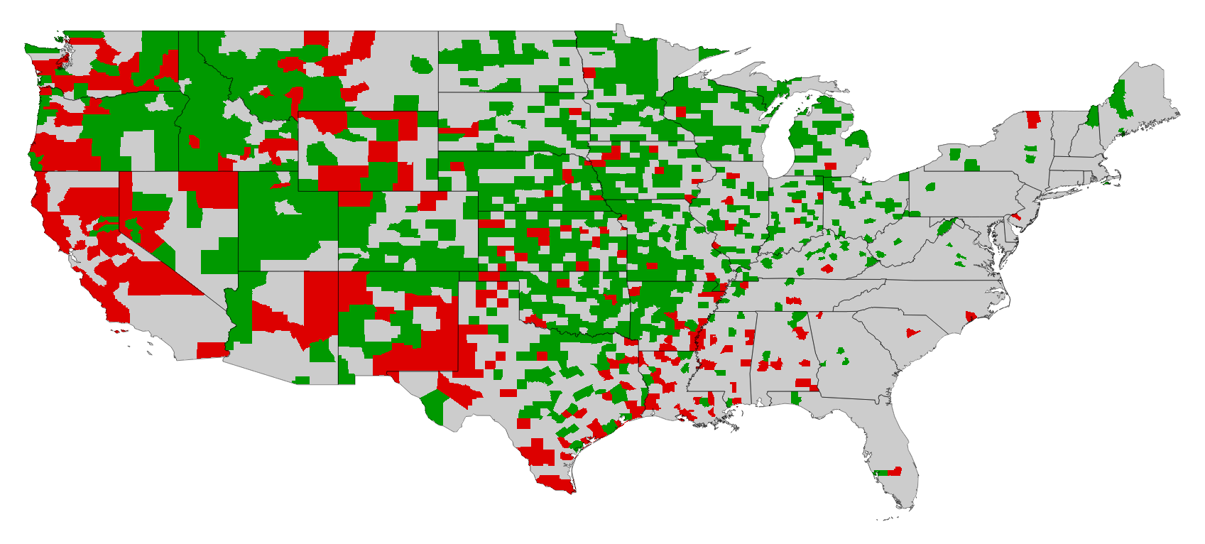
(a) CLSZ, Pair 1

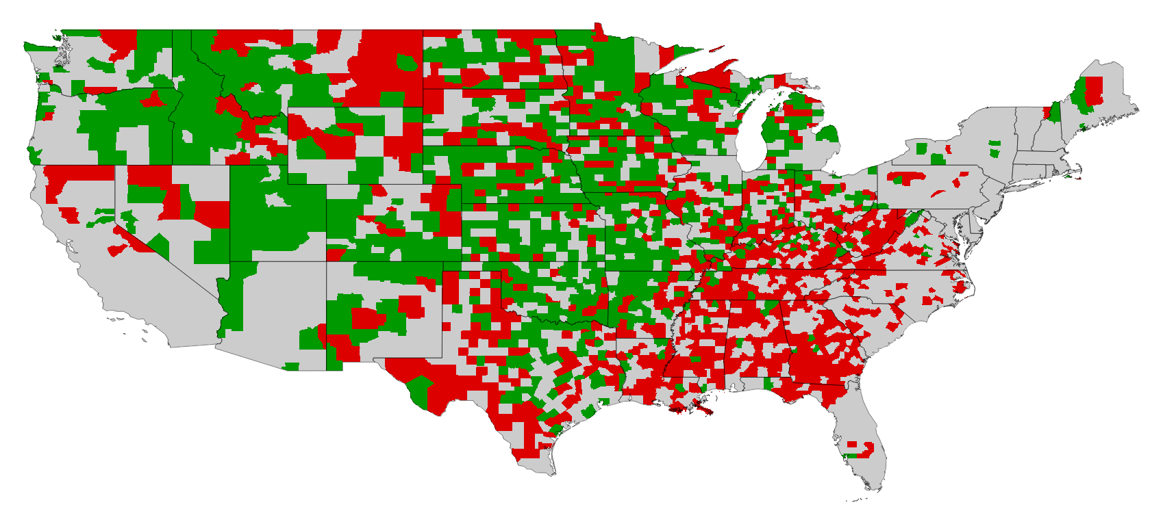
(b) CLSZ, Pair 2

(c) CLSZ, Pair 3

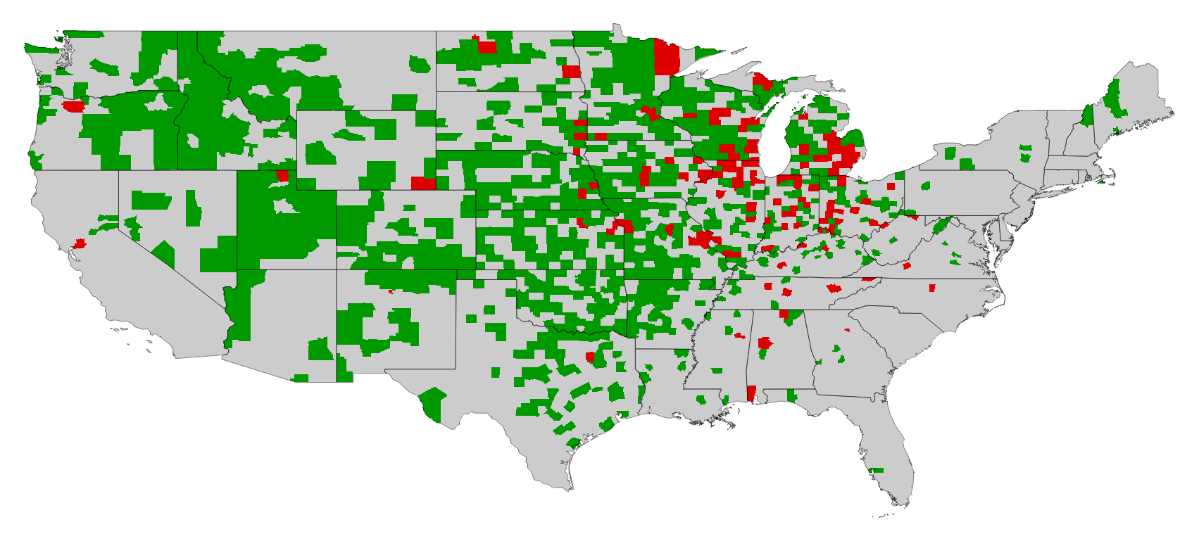
(d) CLSZ, Pair 4

Figure 8: The top $4$ pairs of clusters found by CLSZ on the US Migration dataset.

These experiments suggest that local algorithms are not only more efficient, but can also be much more effective than global algorithms when learning certain structures in graphs. In particular, some localised structure might be hidden when applying the objective function over the entire graph.

Appendix A Omitted detail from Section 3

In this section, we present all the omitted details from Section 3 of our paper. We formally introduce the Lovász-Simonovits curve and use it to analyse the performance of the LocBipartDC algorithm for undirected graphs.

The Lovász-Simonovits Curve.

Our analysis of the LocBipartDC algorithm is based on the Lovász-Simonovits curve, which has been used extensively in the analysis of local clustering algorithms [4, 32]. Lovász and Simonovits [17] originally defined the following function to reason about the mixing rate of Markov chains. For any vector $p\in\mathbb{R}_{\geq 0}^{n}$, we order the vertices such that

$$\frac{p(v_{1})}{\deg(v_{1})}\geq\frac{p(v_{2})}{\deg(v_{2})}\geq\ldots\geq\frac{p(v_{n})}{\deg(v_{n})},$$

and define the sweep sets of $p$ as $S_{j}^{p}=\{v_{1},\ldots,v_{j}\}$ for $1\leq j\leq n$. The Lovász-Simonovits curve, denoted by $p[x]$ for $x\in[0,\mathrm{vol}(V)]$, is defined by the points $p[\mathrm{vol}(S_{j}^{p})]\triangleq p(S_{j}^{p}),$ and is linear between those points for consecutive $j$. Lovász and Simonovits also show that

$$p\!\left[x\right]=\max_{\begin{subarray}{c}w\in[0,1]^{n}\\ \sum_{u\in V}w(u)\deg(u)=x\end{subarray}}\sum_{u\in V}w(u)p(u).$$ (2)

Proposition 1.

For any $p\in\mathbb{R}_{\geq 0}^{n}$ and any $S\subseteq V$, it holds that $p(S)\leq p\!\left[\mathrm{vol}(S)\right].$

Proof.

By definition, we have that $p(S)=\sum_{u\in V}\chi_{S}(u)p(u).$ Hence, by (2) we have that $p(S)\leq p\!\left[\mathrm{vol}(S)\right]$. ∎

Double Cover Reduction.

The following two proofs establish the reduction from almost-bipartite sets to sets with low conductance in the double cover and follow almost directly from the definition of the bipartiteness ratio and conductance.

Proof of Lemma 1.

Let $S^{\prime}=L_{1}\cup R_{2}$, and by definition we have that $\mathrm{vol}_{G}(S)=\mathrm{vol}_{H}(S^{\prime})$. On the other hand, it holds that

$$\mathrm{vol}_{H}(S^{\prime})=e_{H}(S^{\prime},V\setminus S^{\prime})+2e_{H}(S^{\prime},S^{\prime})=e_{H}(S^{\prime},V\setminus S^{\prime})+2e_{H}(L_{1},R_{2}),$$

which implies that

$$\Phi_{H}(S^{\prime})=\frac{e_{H}(S^{\prime},V\setminus S^{\prime})}{\mathrm{vol}_{H}(S^{\prime})}=\frac{\mathrm{vol}_{G}(S)-2e_{H}(L_{1},R_{2})}{\mathrm{vol}_{G}(S)}=1-\frac{2e_{G}(L,R)}{\mathrm{vol}_{G}(S)}=\beta_{G}(L,R),$$

which proves the statement. ∎

Proof of Lemma 2.

The statement follows by Lemma 1. ∎

The simplify operator.

We now study the $\sigma$-operator to establish the properties given in Lemma 3. Recall that the lazy random walk matrix for a graph is defined to be $W=\frac{1}{2}(I+D^{-1}A)$.

Proof of Lemma 3.

For any $u_{1}\in V_{H}$, we have by definition that

$$\sigma\circ(c\cdot p)(u_{1}) =\max(0,c\cdot p(u_{1})-c\cdot p(u_{2}))$$

$$=c\cdot\max(0,p(u_{1})-p(u_{2}))$$

$$=c\cdot\sigma\circ p(u_{1}),$$

and similarly we have $\sigma\circ(c\cdot p)(u_{2})=c\cdot\sigma\circ p(u_{2})$. Therefore, the first property holds.

Now we prove the second statement. Let $u_{1},u_{2}\in V_{H}$ be the vertices that correspond to $u\in V_{G}$. We have by definition that

$$\sigma\circ(a+b)(u_{1}) =\max(0,a(u_{1})+b(u_{1})-a(u_{2})-b(u_{2}))$$

$$=\max(0,a(u_{1})-a(u_{2})+b(u_{1})-b(u_{2}))$$

$$\leq\max(0,a(u_{1})-a(u_{2}))+\max(0,b(u_{1})-b(u_{2}))$$

$$=\sigma\circ a(u_{1})+\sigma\circ b(u_{1}),$$

where the last inequality holds by the fact that $\max(0,x+y)\leq\max(0,x)+\max(0,y)$ for any $x,y\in\mathbb{R}$. For the same reason, we have that

$$\sigma\circ(a+b)(u_{2})\leq\sigma\circ a(u_{2})+\sigma\circ b(u_{2}).$$

Combining these proves the second property of $\sigma$.

Finally, we will prove the third property. By the definition of matrix $W$, we have that

$$(pW)(u_{1})=\frac{1}{2}p(u_{1})+\frac{1}{2}\sum_{v\in N_{G}(u)}\frac{p(v_{2})}{\deg_{H}(v_{2})},$$

and

$$(pW)(u_{2})=\frac{1}{2}p(u_{2})+\frac{1}{2}\sum_{v\in N_{G}(u)}\frac{p(v_{1})}{\deg_{H}(v_{1})}.$$

Without loss of generality, we assume that $(pW)(u_{1})\geq(pW)(u_{2})$. This implies that $(\sigma\circ(pW))(u_{2})=0\leq((\sigma\circ p)W)(u_{2})$, hence it suffices to prove that $(\sigma\circ(pW))(u_{1})\leq((\sigma\circ p)W)(u_{1})$. By definition, we have that

$$(\sigma\circ(pW))(u_{1}) =\max(0,pW(u_{1})-pW(u_{2}))$$

$$=pW(u_{1})-pW(u_{2})$$

$$=\frac{1}{2}\left(p(u_{1})-p(u_{2})\right)+\frac{1}{2}\sum_{v\in N_{G}(u)}\left(\frac{p(v_{2})}{\deg_{H}(v_{2})}-\frac{p(v_{1})}{\deg_{H}(v_{1})}\right)$$

$$=\frac{1}{2}\left(p(u_{1})-p(u_{2})\right)+\frac{1}{2}\sum_{v\in N_{G}(u)}\frac{p(v_{2})-p(v_{1})}{\deg_{G}(v)},$$ (3)

where the last line follows by the fact that $\deg_{H}(v_{1})=\deg_{H}(v_{2})=\deg_{G}(v)$ for any $v\in V_{G}$. To analyse (3), notice that $p(v_{1})-p(v_{2})=(\sigma\circ p)(v_{1})-(\sigma\circ p)(v_{2})$ for any $v\in V_{G}$ for the following reasons:

• When $p(v_{1})\geq p(v_{2})$, we have that $(\sigma\circ p)(v_{1})-(\sigma\circ p)(v_{2})=\left(p(v_{1})-p(v_{2})\right)-0=p(v_{1})-p(v_{2})$;

• Otherwise, we have $p(v_{1})<p(v_{2})$ and $(\sigma\circ p)(v_{1})-(\sigma\circ p)(v_{2})=0-(p(v_{2})-p(v_{1}))=p(v_{1})-p(v_{2})$.

Therefore, we can rewrite (3) as

$$(\sigma\circ(pW))(u_{1}) =\frac{1}{2}((\sigma\circ p)(u_{1})-(\sigma\circ p)(u_{2}))+\frac{1}{2}\sum_{v\in N(u)}\frac{(\sigma\circ p)(v_{2})-(\sigma\circ p)(v_{1})}{\deg_{G}(v)}$$

$$\leq\frac{1}{2}\cdot(\sigma\circ p)(u_{1})+\frac{1}{2}\sum_{v\in N(u)}\frac{(\sigma\circ p)(v_{2})}{\deg_{G}(v)}$$

$$=((\sigma\circ p)W)(u_{1}),$$

where the inequality holds by the fact that $(\sigma\circ p)(u_{1})\geq 0$ and $(\sigma\circ p)(u_{2})\geq 0$ for any $u\in V_{G}$. Since the analysis above holds for any $v\in V_{G}$, we have that $\sigma\circ(pW)\preceq(\sigma\circ p)W$, which finishes the proof of the statement. ∎

Analysis of ApproximatePagerankDC.

The following lemma shows that dcpush maintains that throughout the algorithm, $\left[p_{1},p_{2}\right]$ is an approximate Pagerank vector on the double cover with residual $\left[r_{1},r_{2}\right]$.

Lemma 8.

Let $p^{\prime}_{1},p^{\prime}_{2},r^{\prime}_{1}$ and $r^{\prime}_{2}$ be the result of $\texttt{dcpush}((u,i),p_{1},p_{2},r_{1},r_{2})$. Let $p=\left[p_{1},p_{2}\right]$, $r=\left[r_{1},r_{2}\right]$, $p^{\prime}=\left[p^{\prime}_{1},p^{\prime}_{2}\right]$ and $r^{\prime}=\left[r^{\prime}_{1},r^{\prime}_{2}\right]$. Then, we have that

$$p^{\prime}+\mathrm{pr}_{H}(\alpha,r^{\prime})=p+\mathrm{pr}_{H}(\alpha,r).$$

Proof.

After the push operation, we have

$$p^{\prime} =p+\alpha r(u_{i})\chi_{u_{i}}$$

$$r^{\prime} =r-r(u_{i})\chi_{u_{i}}+(1-\alpha)r(u_{i})\chi_{u_{i}}W$$

where $W$ is the lazy random walk matrix on the double cover of the input graph. Then we have

$$p+\mathrm{pr}_{H}(\alpha,r) =p+\mathrm{pr}_{H}(\alpha,r-r(u_{i})\chi_{u_{i}})+\mathrm{pr}_{H}(\alpha,r(u_{i})\chi_{u_{i}})$$

$$=p+\mathrm{pr}_{H}(\alpha,r-r(u_{i})\chi_{u_{i}})+\left[\alpha r(u)\chi_{u_{i}}+(1-\alpha)\mathrm{pr}_{H}(\alpha,r(u)\chi_{u_{i}}W)\right]$$

$$=\left[p+\alpha r(u_{i})\chi_{u_{i}}\right]+\mathrm{pr}_{H}(\alpha,\left[r-r(u_{i})\chi_{u_{i}}+(1-\alpha)r(u_{i})\chi_{u_{i}}W\right])$$

$$=p^{\prime}+\mathrm{pr}_{H}(\alpha,r^{\prime}),$$

where we use the fact that $\mathrm{pr}(\alpha,\cdot)$ is linear and that

$$\mathrm{pr}(\alpha,s)=\alpha s+(1-\alpha)\mathrm{pr}(\alpha,sW),$$

which follows from the fact that $\mathrm{pr}(\alpha,s)=\alpha\sum_{t=0}^{\infty}(1-\alpha)^{t}sW^{t}$. ∎

The following lemma shows the correctness and performance guarantee of the ApproximatePagerankDC algorithm.

Lemma 9.

For a graph $G$ with double cover $H$ and any $v\in V_{G}$, $\texttt{ApproximatePagerankDC}(v,\alpha,\epsilon)$ runs in time $O(\frac{1}{\epsilon\alpha})$ and computes $p=\mathrm{apr}_{H}(\alpha,\chi_{v_{1}},r)$ such that $\max_{u\in V_{H}}\frac{r(u)}{\deg(u)}<\epsilon$ and $\mathrm{vol}(\mathrm{supp}(p)))\leq\frac{1}{\epsilon\alpha}$.

Proof.

By Lemma 8, we have that $p=\mathrm{apr}_{H}(\alpha,\chi_{v_{1}},r)$ throughout the algorithm and so this clearly holds for the output vector. By the stopping condition of the algorithm, it is clear that $\max_{u\in V_{H}}\frac{r(u)}{\mathrm{deg}(u)}<\epsilon$.

Let $T$ be the total number of push operations performed by ApproximatePagerankDC, and let $d_{j}$ be the degree of the vertex $u_{i}$ used in the $j$th push. The amount of probability mass on $u_{i}$ at time $j$ is at least $\epsilon d_{j}$ and so the amount of probability mass that moves from $r_{i}$ to $p_{i}$ at step $j$ is at least $\alpha\epsilon d_{i}$. Since $\|r_{1}\|_{1}+\|r_{2}\|_{1}=1$ at the beginning of the algorithm, we have that $\alpha\epsilon\sum_{j=1}^{T}d_{j}\leq 1,$ which implies that

$$\sum_{j=1}^{T}d_{j} \leq\frac{1}{\alpha\epsilon}.$$ (4)

Now, note that for every vertex in $\mathrm{supp}(p)$, there must have been at least one push operation on that vertex. So,

$$\mathrm{vol}(\mathrm{supp}(p))=\sum_{v\in\mathrm{supp}(p)}d(v)\leq\sum_{j=1}^{T}d_{j}\leq\frac{1}{\epsilon\alpha}.$$

Finally, to bound the running time, we can implement the algorithm by maintaining a queue of vertices satisfying $\frac{r(u)}{d(u)}\geq\epsilon$ and repeat the push operation on the first item in the queue at every iteration, updating the queue as appropriate. The push operation and queue updates can be performed in time proportional to $d(u)$ and so the running time follows from (4). ∎

Analysis of LocBipartDC.

We will make use of the following fact proved by Andersen et al. [4] which shows that the approximate Pagerank vector will have a large probability mass on a set of vertices if they have low conductance.

Proposition 2 ([4], Theorem 4).

For any vertex set $S$ and any constant $\alpha\in[0,1]$, there is a subset $S_{\alpha}\subseteq S$ with $\mathrm{vol}(S_{\alpha})\geq\mathrm{vol}(S)/2$ such that for any vertex $v\in S_{\alpha}$, the approximate PageRank vector $\mathrm{apr}(\alpha,\chi_{v},r)$ satisfies

$$\mathrm{apr}(\alpha,\chi_{v},r)(S)\geq 1-\frac{\Phi(S)}{\alpha}-\mathrm{vol}(S)\max_{u\in V}\frac{r(u)}{\deg(u)}.$$

The following proof generalises this result to show that applying the $\sigma$-operator to the approximate Pagerank vector maintains this large probability mass, up to a constant factor.

Proof of Lemma 4.

By Lemma 1 and Proposition 2, there is a set $S_{\alpha}\subseteq S$ with $\mathrm{vol}(S_{\alpha})\geq\mathrm{vol}(S)/2$ such that it holds for $v\in S_{\alpha}$ that

$$\mathrm{apr}_{H}(\alpha,\chi_{v},r)(L_{1}\cup R_{2})\geq 1-\frac{\beta(L,R)}{\alpha}-\mathrm{vol}(S)\max_{u\in V}\frac{r(u)}{\deg(u)}.$$

Therefore, by the definition of $p$ we have that

$$p(L_{1}\cup R_{2}) \geq\mathrm{apr}(\alpha,\chi_{v},r)(L_{1}\cup R_{2})-\mathrm{apr}(\alpha,\chi_{v},r)(L_{2}\cup R_{1})$$

$$\geq\mathrm{apr}(\alpha,\chi_{v},r)(L_{1}\cup R_{2})-\mathrm{apr}(\alpha,\chi_{v},r)(\overline{L_{1}\cup R_{2}})$$

$$\geq\mathrm{apr}(\alpha,\chi_{v},r)(L_{1}\cup R_{2})-(1-\mathrm{apr}(\alpha,\chi_{v},r)(L_{1}\cup R_{2}))$$

$$=2\cdot\mathrm{apr}(\alpha,\chi_{v},r)(L_{1}\cup R_{2})-1$$

$$\geq 1-\frac{2\beta(L,R)}{\alpha}-2\mathrm{vol}(S)\max_{u\in V}\frac{r(u)}{\deg(u)},$$

which proves the statement of the lemma. ∎

For the proof of Lemma 5, we need to carefully analyse the effect of the $\sigma$-operator on the approximate Pagerank vector, and in particular notice the effect of the residual vector $r$.

Proof of Lemma 5.

Let $u\in V_{G}$ be an arbitrary vertex. We have that

$$p(u_{1})$$

$$=\sigma\circ\big{(}\mathrm{pr}(\alpha,s)-\mathrm{pr}(\alpha,r)\big{)}(u_{1})$$

$$=\sigma\circ\big{(}\alpha s+(1-\alpha)\mathrm{pr}(\alpha,s)W-\alpha r-(1-\alpha)\mathrm{pr}(\alpha,r)W\big{)}(u_{1})$$

$$=\sigma\circ\big{(}\alpha s+(1-\alpha)\mathrm{apr}(\alpha,s,r)W-\alpha r\big{)}(u_{1})$$

$$=\max\Big{(}0,\big{(}\alpha s+(1-\alpha)\mathrm{apr}(\alpha,s,r)W\big{)}(u_{1})-\big{(}\alpha s+(1-\alpha)\mathrm{apr}(\alpha,s,r)W\big{)}(u_{2})+\alpha r(u_{2})-\alpha r(u_{1})\Big{)}$$

$$\leq\sigma\circ\big{(}\alpha s+(1-\alpha)\mathrm{apr}(\alpha,s,r)W\big{)}(u_{1})+\max(0,\alpha r(u_{2})-\alpha r(u_{1}))$$

$$\leq\sigma\circ\big{(}\alpha s+(1-\alpha)\mathrm{apr}(\alpha,s,r)W\big{)}(u_{1})+\alpha r(u_{2})$$

$$\leq\sigma\circ\big{(}\alpha s\big{)}(u_{1})+(1-\alpha)\sigma\circ\big{(}\mathrm{apr}(\alpha,s,r)W\big{)}(u_{1})+\alpha r(u_{2})$$

$$\leq\alpha s(u_{1})+\alpha r(u_{2})+(1-\alpha)(pW)(u_{1}),$$

where the first line follows by the definition of the approximate Pagerank, the second line follows by the definition of the Pagerank, and the last two inequalities follow by Lemma 3. This proves the first inequality, and the second inequality follows by symmetry. ∎

We now turn our attention to the Lovász-Simonovits curve defined by the simplified approximate Pagerank vector $p=\sigma\circ\mathrm{apr}(\alpha,s,r)$. We will bound the curve at some point by the conductance of the corresponding sweep set with the following lemma.

Lemma 10.

Let $p=\sigma\circ\left(\mathrm{apr}(\alpha,s,r)\right)$. It holds for any $j\in[1,n-1]$ that

$$p\!\left[\mathrm{vol}(S_{j}^{p})\right]$$

$$\leq \alpha\Big{(}s\!\left[\mathrm{vol}(S_{j}^{p})\right]+r\!\left[\mathrm{vol}(S_{j}^{p})\right]\Big{)}+(1-\alpha)\frac{1}{2}\Big{(}p\!\left[\mathrm{vol}(S_{j}^{p})-\left\lvert\partial(S_{j}^{p})\right\rvert\right]\Big{)}+(1-\alpha)\frac{1}{2}\Big{(}p\!\left[\mathrm{vol}(S_{j}^{p})+\left\lvert\partial(S_{j}^{p})\right\rvert\right]\Big{)}.$$

Since $\mathrm{vol}(S_{j}^{p})\pm\left\lvert\partial(S_{j}^{p})\right\rvert=\mathrm{vol}(S_{j}^{p})(1\pm\Phi(S_{j}^{p}))$, this tells us that when the conductance of the sweep set $S_{j}^{p}$ is large, the Lovász-Simonovits curve around the point $\mathrm{vol}(S_{j}^{p})$ is close to a straight line. For the proof of Lemma 10, we will view the undirected graph $H$ instead as a digraph, and each edge $\{u,v\}\in E_{H}$ as a pair of directed edges $(u,v)$ and $(v,u)$. For any edge $(u,v)$ and vector $p\in\mathbb{R}_{\geq 0}^{2n}$, let

$$p(u,v)=\frac{p(u)}{d(u)}$$

and for a set of directed edges $A$, let

$$p(A)=\sum_{(u,v)\in A}p(u,v).$$

Now for any set of vertices $S\subset V_{H}$, let $\mathrm{in}(S)=\{(u,v)\in E_{H}:v\in S\}$ and $\mathrm{out}(S)=\{(u,v)\in E_{H}:u\in S\}$. Additionally, for any simple set $S\subset V_{H}$, we define the “simple complement” of the set $S$ by

$$\widehat{S}=\{u_{2}:u_{1}\in S\}\cup\{u_{1}:u_{2}\in S\}.$$

We will need the following property of the Lovász-Simonovitz curve with regard to sets of edges.

Lemma 11.

For any set of edges $A$, it holds that

$$p(A)\leq p\!\left[\left\lvert A\right\rvert\right].$$

Proof.

For each $u\in V$, let $x_{u}=\left\lvert\{(u,v)\in A\}\right\rvert$ be the number of edges in $A$ with the tail at $u$. Then, we have by definition that

$$p(A) =\sum_{(u,v)\in A}\frac{p(u)}{d(u)}=\sum_{u\in V}\frac{x_{u}}{d(u)}p(u)$$

Since $\frac{x_{u}}{d(u)}\in[0,1]$ and

$$\sum_{u\in V}\frac{x_{u}}{d(u)}d(u)=\sum_{u\in V}x_{u}=\left\lvert A\right\rvert,$$

the statement follows from equation (2). ∎

We will also make use of the following lemma from [4].

Lemma 12 ([4], Lemma 4).

For any distribution $p$, and any set of vertices $A$,

$$pW(A)\leq\frac{1}{2}\cdot\left(p(\mathrm{in}(A)\cup\mathrm{out}(A))+p(\mathrm{in}(A)\cap\mathrm{out}(A))\right)$$

We now have all the pieces we need to prove the behaviour of the Lovász-Simonovits curve described in Lemma 10.

Proof of Lemma 10.

By definition, we have that

$$p(S)$$

$$=\sum_{u_{1}\in S}p(u_{1})+\sum_{u_{2}\in S}p(u_{2})$$

$$\leq\sum_{u_{1}\in S}\Big{(}\alpha\left(s(u_{1})+r(u_{2})\right)+(1-\alpha)(pW)(u_{1})\Big{)}+\sum_{u_{2}\in S}\Big{(}\alpha\left(s(u_{2})+r(u_{1})\right)+(1-\alpha)(pW)(u_{2})\Big{)}$$

$$=\alpha\cdot\Bigg{(}\sum_{u_{1}\in S}s(u_{1})+\sum_{u_{2}\in S}s(u_{2})+\sum_{u_{1}\in S}r(u_{2})+\sum_{u_{2}\in S}r(u_{1})\Bigg{)}+(1-\alpha)\cdot\Bigg{(}\sum_{u_{1}\in S}(pW)(u_{1})+\sum_{u_{2}\in S}(pW)(u_{2})\Bigg{)}$$

$$=\alpha\cdot\Big{(}s(S)+r\left(\widehat{S}\right)\!\Big{)}+(1-\alpha)\cdot pW(S)$$

$$\leq\alpha\cdot\Big{(}s(S)+r\left(\widehat{S}\right)\!\Big{)}+(1-\alpha)\cdot\frac{1}{2}\cdot\Big{(}p(\mathrm{in}(S)\cup\mathrm{out}(S))+p(\mathrm{in}(S)\cap\mathrm{out}(S))\Big{)},$$

where the first inequality follows by Lemma 5 and the last inequality follows by Lemma 12.

Now, recall that $p\!\left[\mathrm{vol}(S_{j}^{p})\right]=p(S_{j}^{p})$ and notice that $\mathrm{vol}\left(\widehat{S_{j}^{p}}\right)=\mathrm{vol}\left(S_{j}^{p}\right)$ holds by the definition of $\widehat{S}$. Hence, using Lemma 11, we have that

$$p\!\left[\mathrm{vol}(S_{j}^{p})\right]$$

$$=p(S_{j}^{p})$$

$$\leq\alpha\left(s(S_{j}^{p})+r\left(\widehat{S_{j}^{p}}\right)\right)+(1-\alpha)\cdot\frac{1}{2}\Big{(}p\left(\mathrm{in}(S_{j}^{p})\cup\mathrm{out}(S_{j}^{p})\right)+p(\mathrm{in}(S_{j}^{p})\cap\mathrm{out}(S_{j}^{p}))\Big{)}$$

$$\leq\alpha\Big{(}s\!\left[\mathrm{vol}(S_{j}^{p})\right]+r\!\left[\mathrm{vol}(S_{j}^{p})\right]\Big{)}+(1-\alpha)\cdot\frac{1}{2}\left(p\!\left[\left\lvert\mathrm{in}(S_{j}^{p})\cup\mathrm{out}(S_{j}^{p})\right\rvert\right]+p\!\left[\left\lvert\mathrm{in}(S_{j}^{p})\cap\mathrm{out}(S_{j}^{p})\right\rvert\right]\right).$$

It remains to show that

$$\left\lvert\mathrm{in}(S_{j}^{p})\cap\mathrm{out}(S_{j}^{p})\right\rvert=\mathrm{vol}(S_{j}^{p})-\left\lvert\partial(S_{j}^{p})\right\rvert,$$

and

$$\left\lvert\mathrm{in}(S_{j}^{p})\cup\mathrm{out}(S_{j}^{p})\right\rvert=\mathrm{vol}(S_{j}^{p})+\left\lvert\partial(S_{j}^{p})\right\rvert.$$

The first follows by noticing that $\left\lvert\mathrm{in}(S_{j}^{p})\cap\mathrm{out}(S_{j}^{p})\right\rvert$ counts precisely twice the number of edges with both endpoints inside $S_{j}^{p}$. The second follows since

$$\left\lvert\mathrm{in}(S_{j}^{p})\cup\mathrm{out}(S_{j}^{p})\right\rvert=\left\lvert\mathrm{in}(S_{j}^{p})\cap\mathrm{out}(S_{j}^{p})\right\rvert+\left\lvert\mathrm{in}(S_{j}^{p})\setminus\mathrm{out}(S_{j}^{p})\right\rvert+\left\lvert\mathrm{out}(S_{j}^{p})\setminus\mathrm{in}(S_{j}^{p})\right\rvert$$

and both the second and third terms on the right hand side are equal to $\left\lvert\partial(S_{j}^{p})\right\rvert$. ∎

To understand the following lemma, notice that since $p[0]=0$ and $p[\mathrm{vol}(H)]=1$, if the curve were simply linear then it would be the case that $p[k]=\frac{k}{\mathrm{vol}(H)}$ and so the following lemma bounds how far the Lovász-Simonovits curve deviates from this line. In particular, if there is no sweep set with small conductance, then the deviation must be small.

Lemma 13.

Let $p=\sigma\circ\left(\mathrm{apr}_{H}(\alpha,s,r)\right)$ such that $\max_{u\in V_{H}}\frac{r(u)}{d(u)}\leq\epsilon$, and $\phi$ be any constant in $[0,1]$. If $\Phi(S_{j}^{p})\geq\phi$ for all $j\in[1,\left\lvert\mathrm{supp}(p)\right\rvert]$, then

$$p[k]-\frac{k}{\mathrm{vol}(H)}\leq\alpha t+\alpha\epsilon kt+\sqrt{\min(k,\mathrm{vol}(H)-k)}\left(1-\frac{\phi^{2}}{8}\right)^{t}$$

for all $k\in[0,\mathrm{vol}(H)]$ and integer $t\geq 0$.

Proof.

For ease of discussion we write $k_{j}=\mathrm{vol}(S_{j}^{p})$ and let $\overline{k_{j}}=\min(k_{j},\mathrm{vol}(H)-k_{j})$. For convenience we will write

$$f_{t}(k)=\alpha t+\alpha\epsilon kt+\sqrt{\min(k,\mathrm{vol}(H)-k)}\left(1-\frac{\phi^{2}}{8}\right)^{t}.$$

We will prove by induction that for all $t\geq 0$,

$$p[k]-\frac{k}{\mathrm{vol}(H)}\leq f_{t}(k).$$

For the base case, this equation holds for $t=0$ for any $\phi$. Our proof is based on a case distinction: (1) For any integer $k\in[1,\mathrm{vol}(H)-1]$,

$$p[k]-\frac{k}{\mathrm{vol}(H)}\leq 1\leq\sqrt{\min(k,\mathrm{vol}(H)-k)}\leq f_{0}(k);$$

(2) For $k=0$ or $k=\mathrm{vol}(H)$, $p[k]-\frac{k}{\mathrm{vol}(H)}=0\leq f_{0}(k)$. The base case follows since $f_{0}$ is concave, and $p[k]$ is linear between integer values.

Now for the inductive case, we assume that the claim holds for $t$ and will show that it holds for $t+1$. It suffices to show that the following holds for every $j\in[1,\left\lvert\mathrm{supp}(p)\right\rvert]$:

$$p[k_{j}]-\frac{k_{j}}{\mathrm{vol}(H)}\leq f_{t+1}(k_{j}).$$

The theorem will follow because this equation holds trivially for $j=0$ and $j=n$ and $p[k]$ is linear between $k_{j}$ for $j\in\{0,n\}\cup[1,|\mathrm{supp}(p)|]$.

For any $j\in[1,|\mathrm{supp}(p)|]$, it holds by Lemma 10 that

$$p\!\left[k_{j}\right] \leq\alpha\left(s\!\left[k_{j}\right]+r\!\left[k_{j}\right]\right)+(1-\alpha)\frac{1}{2}\left(p\!\left[k_{j}-\left\lvert\partial(S_{j}^{p})\right\rvert\right]+p\!\left[k_{j}+\left\lvert\partial(S_{j}^{p})\right\rvert\right]\right)$$

$$\leq\alpha+\alpha\epsilon k_{j}+\frac{1}{2}\left(p\!\left[k_{j}-\Phi(S_{j}^{p})\cdot\overline{k_{j}}\right]+p\!\left[k_{j}+\Phi(S_{j}^{p})\cdot\overline{k_{j}}\right]\right)$$

$$\leq\alpha+\alpha\epsilon k_{j}+\frac{1}{2}\left(p\!\left[k_{j}-\phi\overline{k_{j}}\right]+p\!\left[k_{j}+\phi\overline{k_{j}}\right]\right),$$

where the second line uses the fact that $r\!\left[k_{j}\right]\leq\epsilon k_{j}$ and the last line uses the concavity of $p\!\left[k\right]$ and the fact that $\Phi(S_{j}^{p})\geq\phi$. By the induction hypothesis, we have that

$$p\!\left[k_{j}\right]$$

$$\leq\alpha+\alpha\epsilon k_{j}+\frac{1}{2}\left(f_{t}(k_{j}-\phi\overline{k_{j}})+\frac{k_{j}-\phi\overline{k_{j}}}{\mathrm{vol}(H)}+f_{t}(k_{j}+\phi\overline{k_{j}})+\frac{k_{j}+\phi\overline{k_{j}}}{\mathrm{vol}(H)}\right)$$

$$=\alpha+\alpha\epsilon k_{j}+\frac{k_{j}}{\mathrm{vol}(H)}+\frac{1}{2}\left(f_{t}(k_{j}+\phi\overline{k_{j}})+f_{t}(k_{j}-\phi\overline{k_{j}})\right)$$

$$\!\begin{aligned} &=\alpha+\alpha\epsilon k_{j}+\alpha t+\alpha\epsilon k_{j}t+\frac{k_{j}}{\mathrm{vol}(H)}\\ &\qquad+\frac{1}{2}\left(\sqrt{\min(k_{j}-\phi\overline{k_{j}},\mathrm{vol}(H)-k_{j}+\phi\overline{k_{j}})}+\sqrt{\min(k_{j}+\phi\overline{k_{j}},\mathrm{vol}(H)-k_{j}-\phi\overline{k_{j}})}\right)\left(1-\frac{\phi^{2}}{8}\right)^{t}\end{aligned}$$

$$\leq\alpha(t+1)+\alpha\epsilon k_{j}(t+1)+\frac{k_{j}}{\mathrm{vol}(H)}+\frac{1}{2}\left(\sqrt{\overline{k_{j}}-\phi\overline{k_{j}}}+\sqrt{\overline{k_{j}}+\phi\overline{k_{j}}}\right)\left(1-\frac{\phi^{2}}{8}\right)^{t}$$

Now, using the Taylor series of $\sqrt{1+\phi}$ at $\phi=0$, we see the following for any $x\geq 0$ and $\phi\in[0,1]$.

$$\frac{1}{2}\left(\sqrt{x-\phi x}+\sqrt{x+\phi x}\right) \leq\frac{\sqrt{x}}{2}\left(\left(1-\frac{\phi}{2}-\frac{\phi^{2}}{8}-\frac{\phi^{3}}{16}\right)+\left(1+\frac{\phi}{2}-\frac{\phi^{2}}{8}+\frac{\phi^{3}}{16}\right)\right)$$

$$\leq\sqrt{x}\left(1-\frac{\phi^{2}}{8}\right).$$

Applying this with $x=\overline{k_{j}}$, we have

$$p\!\left[k_{j}\right]-\frac{k_{j}}{\mathrm{vol}(H)} \leq\alpha(t+1)+\alpha\epsilon k_{j}(t+1)+\sqrt{\overline{k_{j}}}\left(1-\frac{\phi^{2}}{8}\right)\left(1-\frac{\phi^{2}}{8}\right)^{t}$$

$$=f_{t+1}(k_{j}),$$

which completes the proof. ∎

The next lemma follows almost directly from Lemma 13 by carefully choosing the value of $t$.

Proof of Lemma 6.

Let $H_{c}$ be a weighted version of the double cover with the weight of every edge equal to some constant $c$. Let $k=\mathrm{vol}_{H_{c}}(S)$ and $\overline{k}=\min(k,\mathrm{vol}(H_{c})-k)$. Notice that the behaviour of random walks and the conductance of vertex sets are unchanged by re-weighting the graph by a constant factor. As such, $p=\sigma\circ\mathrm{apr}_{H_{c}}(\alpha,s,r)$ and we let $\phi=\min_{j}\Phi_{H_{c}}(S_{j}^{p})$. Hence, by Lemma 13 it holds for any $t>0$ that

$$\delta <p\!\left[k\right]-\frac{k}{\mathrm{vol}(H_{c})}<\alpha t(1+\epsilon k)+\sqrt{\overline{k}}\left(1-\frac{\phi^{2}}{8}\right)^{t}.$$

Letting $v=\mathrm{vol}(H_{c})$ we set $t=\left\lceil\frac{8}{\phi^{2}}\ln\frac{2\sqrt{v/2}}{\delta}\right\rceil$. Now, assuming that

$$\delta\geq\frac{2}{\sqrt{v/2}}$$ (5)

we have

$$\delta<(1+\epsilon k)\alpha\left\lceil\frac{8}{\phi^{2}}\ln\frac{2\sqrt{v/2}}{\delta}\right\rceil+\frac{\delta}{2\sqrt{v/2}}\sqrt{\overline{k}}<\frac{9(1+\epsilon k)\alpha\ln(v/2)}{\phi^{2}}+\frac{\delta}{2}$$

We set $c$ such that

$$v=c\ \mathrm{vol}(H)=\mathrm{vol}(H_{c})=\left(\frac{4}{\delta}\right)^{2}$$

which satisfies (5) and implies that

$$\phi<\sqrt{\frac{18(1+\epsilon k)\alpha\ln(4/\delta)}{\delta}}.$$

By the definition of $\phi$, there must be some $S_{j}^{p}$ with the desired property. ∎

Finally, we prove the performance guarantees of Algorithm 1 in the following theorem.

Proof of Theorem 1.

We set the parameters of the main algorithm to be

• $\alpha=\widehat{\beta}^{2}/378=20\beta$

• $\epsilon=1/(20\gamma)$.

Let $p=\sigma\circ\left(\mathrm{apr}_{H}(\alpha,\chi_{v},r)\right)$ be the simplified approximate Pagerank vector computed in the algorithm, which satisfies that $\max_{v\in V_{H}}\frac{r(v)}{d(v)}\leq\epsilon$, and let $C^{\prime}=L_{1}\cup R_{2}$ be the target set in the double cover. Hence, by Lemma 4 we have that

$$p(C^{\prime})\geq 1-\frac{2\beta}{\alpha}-2\epsilon\cdot\mathrm{vol}(C)\geq 1-\frac{1}{10}-\frac{1}{10}=\frac{4}{5}.$$

Notice that, since $C^{\prime}$ is simple, we have that $\frac{\mathrm{vol}(C^{\prime})}{\mathrm{vol}(V_{H})}\leq\frac{1}{2}$ and

$$p(C^{\prime})-\frac{\mathrm{vol}(C^{\prime})}{\mathrm{vol}(V_{H})}\geq\frac{4}{5}-\frac{1}{2}=\frac{3}{10}.$$

Therefore, by Lemma 6 and choosing $\delta=3/10$, there is some $j\in[1,\left\lvert\mathrm{supp}(p)\right\rvert]$ such that

$$\Phi(S_{j}^{p}) <\sqrt{\frac{360}{3}(1+\epsilon\mathrm{vol}(C))\alpha\ln(\frac{40}{3})}\leq\sqrt{\left(1+\frac{1}{20}\right)7200\beta}=\widehat{\beta}.$$

Since such a $S_{j}^{p}$ is a simple set, by Lemma 1, we know that the sets $L^{\prime}=\{u\in V_{G}:u_{1}\in S_{j}^{p}\}$ and $R^{\prime}=\{u\in V_{G}:u_{2}\in S_{j}^{p}\}$ satisfy $\beta((,L)^{\prime},R^{\prime})\leq\widehat{\beta}$. For the volume guarantee, Lemma 9 gives that

$$\mathrm{vol}(\mathrm{supp}(p))\leq\frac{1}{\epsilon\alpha}=\frac{\gamma}{\beta}.$$

Since the sweep set procedure in the algorithm is over the support of $p$, we have that

$$\mathrm{vol}(L^{\prime}\cup R^{\prime})\leq\mathrm{vol}(\mathrm{supp}(p))\leq\beta^{-1}\gamma.$$

Now, we will analyse the running time of the algorithm. By Lemma 9, computing the approximate Pagerank vector $p^{\prime}$ takes time

$$O\!\left(\frac{1}{\epsilon\alpha}\right)=O\!\left(\beta^{-1}\gamma\right).$$

Since $\mathrm{vol}(\mathrm{supp}(p^{\prime}))=O\!\left(\frac{1}{\epsilon\alpha}\right)$, computing $\sigma\circ\left(p^{\prime}\right)$ can also be done in time $O\!\left(\beta^{-1}\gamma\right)$. The cost of checking each conductance in the sweep set loop is $O\!\left(\mathrm{vol}(\mathrm{supp}(p))\ln(n)\right)=O\!\left(\beta^{-1}\gamma\ln(n)\right)$. This dominates the running time of the algorithm, which completes the proof of the theorem. ∎

Appendix B Omitted detail from Section 4

In this section, we present all the omitted details from Section 4 of our paper. We will use the evolving set process to analyse the correctness and performance of the EvoCutDirected algorithm.

The evolving set process.

To understand the ESP update process, notice that $\chi_{v}W\chi_{S_{i}}^{\intercal}$ is the probability that a one-step random walk starting at $v$ ends inside $S_{i}$. Given that the transition kernel of the evolving set process is given by $\mathbf{K}(S,S^{\prime})=\mathbb{P}[S_{i+1}=S^{\prime}|S_{i}=S]$, the volume-biased ESP is defined by the transition kernel

$$\mathbf{\widehat{K}}(S,S^{\prime})=\frac{\mathrm{vol}(S^{\prime})}{\mathrm{vol}(S)}\mathbf{K}(S,S^{\prime})$$

We now give some useful facts about the evolving set process which we will use in our analysis of Algorithm 4. The first proposition tells us that an evolving set process running for sufficiently many steps is very likely to have at least one state with low conductance.

Proposition 3 ([6], Corollary 1).

Let $S_{0},S_{1},\ldots,S_{T}$ be sets drawn from the volume-biased evolving set process beginning at $S_{0}$. Then, it holds for any constant $c\geq 0$ that

$$\mathbb{P}\left[\min_{j\leq T}\Phi(S_{j})\leq\sqrt{c}\sqrt{4T^{-1}\ln(\mathrm{vol}(V))}\right]\geq 1-\frac{1}{c}.$$

If $(X_{0},X_{1},\ldots,X_{T})$ is a lazy random walk Markov chain with $X_{0}=x$ then for any set $A\subseteq V_{H}$ and integer $T$, let

$$\mathrm{esc}(x,T,A)\triangleq\mathbb{P}\left[\bigcup_{j=0}^{T}X_{j}\not\in A\right]$$

be the probability that the random walk leaves the set $A$ in the first $T$ steps. We will use the following results connecting the escape probability to the conductance of the set $A$ and the volume of the sets in the evolving set process.

Proposition 4 ([24], Proposition 2.5).

There is a set $A_{T}\subseteq A$ with $\mathrm{vol}(A_{T})\geq\frac{1}{2}\mathrm{vol}(A)$, such that it holds for any $x\in A_{T}$ that

$$\mathrm{esc}(x,T,A)\leq T\Phi(A).$$

Proposition 5 ([6], Lemma 2).

For any vertex $x$, let $S_{0},S_{1},\ldots,S_{T}$ be sampled from a volume-biased ESP starting from $S_{0}=\{x\}$. Then, it holds for any set $A\subseteq V_{H}$ and $\lambda>0$ that

$$\mathbb{P}\left[\max_{t\leq T}\frac{\mathrm{vol}(S_{t}\setminus A)}{\mathrm{vol}(S_{t})}>\lambda\mathrm{esc}(x,T,A)\right]<\frac{1}{\lambda}.$$

Analysis of EvoCutDirected.

We now come to the formal analysis of our algorithm for finding almost-bipartite sets in digraphs. We start by proving the connection between $F(L,R)$ in a digraph with the conductance of the set $L_{1}\cup R_{2}$ in the semi-double cover.

Proof of Lemma 7.

We define $S_{H}=L_{1}\cup R_{2}$, and have that

$$\Phi_{H}(S_{H}) =\frac{e(S_{H},V_{H}\setminus S_{H})}{\mathrm{vol}_{H}(S_{H})}$$

$$=\frac{\mathrm{vol}_{H}(S_{H})-2e_{H}(S_{H},S_{H})}{\mathrm{vol}_{H}(S_{H})}$$

$$=1-\frac{2e_{H}(S_{H},S_{H})}{\mathrm{vol}_{H}(S_{H})}$$

$$=1-\frac{2e_{G}(L,R)}{\mathrm{vol}_{\mathrm{out}}(L)+\mathrm{vol}_{\mathrm{in}}(R)}$$

$$=F_{G}(L,R).$$

This proves the first statement of the lemma. The second statement of the lemma follows by the same argument. ∎

We now show how removing all vertices $u$ where $u_{1}\in S$ and $u_{2}\in S$ affects the conductance of $S$ on the semi-double cover.

Lemma 14.

For any $\epsilon$-simple set $S\subset V_{H}$, let $P=\{u_{1},u_{2}:u\in V_{G},u_{1}\in S\mbox{ and }u_{2}\in S\}$ and set $S^{\prime}=S\setminus P$. Then, $\Phi(S^{\prime})\leq\frac{1}{1-\epsilon}(\Phi(S)+\epsilon).$

Proof.

By the definition of conductance, we have

$$\Phi(S^{\prime}) =\frac{e(S^{\prime},V\setminus S^{\prime})}{\mathrm{vol}(S^{\prime})}$$

$$\leq\frac{e(S,V\setminus S)+\mathrm{vol}(P)}{\mathrm{vol}(S)-\mathrm{vol}(P)}$$

$$\leq\frac{1}{1-\epsilon}\frac{e(S,V\setminus S)+\mathrm{vol}(P)}{\mathrm{vol}(S)}$$

$$\leq\frac{1}{1-\epsilon}\left(\frac{e(S,V\setminus S)}{\mathrm{vol}(S)}+\epsilon\right)$$

$$=\frac{1}{1-\epsilon}\left(\Phi(S)+\epsilon\right),$$

which proves the lemma. ∎

As such, we would like to show that the output of the evolving set process is very close to being a simple set. The following lemma shows that, by choosing the number of steps of the evolving set process carefully, we can very tightly control the overlap of the output of the evolving set process with the target set $S$, which we know to be simple.

Lemma 15.

Let $C\subset V_{H}$ be a set with conductance $\Phi(C)=\phi$, and let $T=(100\phi^{\frac{2}{3}})^{-1}$. There exists a set $C_{g}\subseteq C$ with volume at least $\mathrm{vol}(C)/2$ such that for any $x\in C_{g}$, with probability at least $7/9$, a sample path $(S_{0},S_{1},\ldots,S_{T})$ from the volume-biased ESP started from $S_{0}=\{x\}$ will satisfy the following:

• $\Phi(S_{t})<60\phi^{\frac{1}{3}}\ln^{\frac{1}{2}}\mathrm{vol}(V)$ for some $t\in[0,T]$;

• $\mathrm{vol}(S_{t}\cap C)\geq\left(1-\frac{1}{10}\phi^{\frac{1}{3}}\right)\mathrm{vol}(S_{t})$ for all $t\in[0,T]$.

Proof.

By Proposition 3, with probability at least $(1-1/9)$ there is some $t<T$ such that

$$\Phi(S_{t}) \leq 3\sqrt{4T^{-1}\ln\mathrm{vol}(V_{H})}=3\sqrt{400\phi^{\frac{2}{3}}\ln\mathrm{vol}(V_{H})}=60\phi^{\frac{1}{3}}\ln^{\frac{1}{2}}(\mathrm{vol}(V_{H})).$$

Then, by Proposition 4 we have that $\mathrm{esc}(x,T,C)\leq T\phi=\frac{1}{100}\phi^{1/3}$. Hence, by Proposition 5, with probability at least $9/10$,

$$\max_{t\leq T}\frac{\mathrm{vol}(S_{t}\setminus C)}{\mathrm{vol}(S_{t})}\leq 10\cdot\mathrm{esc}(x,T,C)\leq\frac{1}{10}\cdot\phi^{1/3}$$

Applying the union bound on these two events proves the statement of the lemma. ∎

Now we combine everything together to prove Theorem 2.

Proof of Theorem 2.

By Lemma 15, we know that, with probability at least $7/9$, the set $S$ computed by the algorithm will satisfy

$$\mathrm{vol}(S\cap C)\geq\left(1-\frac{1}{10}\phi^{\frac{1}{3}}\right)\mathrm{vol}(S).$$

Let $P=\{u_{1},u_{2}:u_{1}\in S$ and $u_{2}\in S\}$. Then, since $C$ is simple, we have that

$$\mathrm{vol}(P) \leq 2\cdot(\mathrm{vol}(S)-\mathrm{vol}(S\cap C))\leq 2\cdot\left(1-\left(1-\frac{1}{10}\phi^{\frac{1}{3}}\right)\right)\cdot\mathrm{vol}(S)=\frac{1}{5}\cdot\phi^{\frac{1}{3}}\mathrm{vol}(S),$$

which implies that $S$ is $(1/5)\cdot\phi^{\frac{1}{3}}$-simple. Therefore, by letting $S^{\prime}=S\setminus P$, we have by Lemma 14 that

$$\Phi(S^{\prime}) \leq\frac{1}{1-\epsilon}\cdot\left(\Phi(S)+\epsilon\right)\leq\frac{1}{1-\frac{1}{5}}\left(\Phi(S)+\frac{1}{5}\phi^{\frac{1}{3}}\right)\leq\frac{5}{4}\cdot\Phi(S)+\frac{1}{4}\cdot\phi^{\frac{1}{3}}.$$

Since $\Phi(S)=O\!\left(\phi^{\frac{1}{3}}\ln^{\frac{1}{2}}(n)\right)$ by Lemma 15, we have that $\Phi(S^{\prime})=O\!\left(\phi^{\frac{1}{3}}\ln^{\frac{1}{2}}(n)\right)$. For the volume guarantee, direct calculation shows that

$$\mathrm{vol}(S^{\prime})\leq\mathrm{vol}(S)\leq\frac{\mathrm{vol}(S\cap C)}{1-\frac{1}{10}\phi^{\frac{1}{3}}}\leq\frac{\mathrm{vol}(C)}{1-\phi^{\frac{1}{3}}}.$$

Finally, the running time of the algorithm is dominated by the GenerateSample method, which was shown in [6] to have running time $O\!\left(\mathrm{vol}(C)\phi^{-\frac{1}{2}}\ln^{\frac{3}{2}}(n)\right)$. ∎

References

- [1] Reid Andersen. A local algorithm for finding dense subgraphs. ACM Transactions on Algorithms (TALG), 6(4):1–12, 2010.
- [2] Reid Andersen and Kumar Chellapilla. Finding dense subgraphs with size bounds. In International Workshop on Algorithms and Models for the Web-Graph, pages 25–37, 2009.
- [3] Reid Andersen and Fan Chung. Detecting sharp drops in Pagerank and a simplified local partitioning algorithm. In International Conference on Theory and Applications of Models of Computation (TAMC’07), pages 1–12, 2007.
- [4] Reid Andersen, Fan Chung, and Kevin Lang. Local graph partitioning using Pagerank vectors. In 47th Annual IEEE Symposium on Foundations of Computer Science (FOCS’06), pages 475–486, 2006.
- [5] Reid Andersen, Shayan Oveis Gharan, Yuval Peres, and Luca Trevisan. Almost optimal local graph clustering using evolving sets. Journal of the ACM (JACM), 63(2):1–31, 2016.
- [6] Reid Andersen and Yuval Peres. Finding sparse cuts locally using evolving sets. In 41st Annual ACM Symposium on Theory of Computing (STOC’09), pages 235–244, 2009.
- [7] Austin R. Benson, David F. Gleich, and Jure Leskovec. Tensor spectral clustering for partitioning higher-order network structures. In 15th International Conference on Data Mining (ICDM’15), pages 118–126, 2015.
- [8] Austin R. Benson, David F. Gleich, and Jure Leskovec. Higher-order organization of complex networks. Science, 353(6295):163–166, 2016.
- [9] Michael B Cohen, Jonathan Kelner, John Peebles, Richard Peng, Anup B Rao, Aaron Sidford, and Adrian Vladu. Almost-linear-time algorithms for Markov chains and new spectral primitives for directed graphs. In 49th Annual ACM Symposium on Theory of Computing (STOC’17), pages 410–419, 2017.
- [10] Mihai Cucuringu, Huan Li, He Sun, and Luca Zanetti. Hermitian matrices for clustering directed graphs: Insights and applications. In 23rd International Conference on Artificial Intelligence and Statistics (AISTATS’20), pages 983–992, 2020.
- [11] Kimon Fountoulakis, Di Wang, and Shenghao Yang. -norm flow diffusion for local graph clustering. In 37th International Conference on Machine Learning (ICML’20), pages 3222–3232, 2020.
- [12] Alexander J. Gates and Yong-Yeol Ahn. The impact of random models on clustering similarity. The Journal of Machine Learning Research, 18(1):3049–3076, 2017.
- [13] Changwei Hu, Piyush Rai, and Lawrence Carin. Deep generative models for relational data with side information. In 34th International Conference on Machine Learning (ICML’17), pages 1578–1586, 2017.
- [14] Steinar Laenen and He Sun. Higher-order spectral clustering of directed graphs. In 34th Advances in Neural Information Processing Systems (NeurIPS’20), 2020.
- [15] Angsheng Li and Pan Peng. Detecting and characterizing small dense bipartite-like subgraphs by the bipartiteness ratio measure. In 24th International Symposium on Algorithms and Computation (ISAAC’13), pages 655–665, 2013.
- [16] Meng Liu and David F. Gleich. Strongly local -norm-cut algorithms for semi-supervised learning and local graph clustering. In 34th Advances in Neural Information Processing Systems (NeurIPS’20), 2020.
- [17] László Lovász and Miklós Simonovits. The mixing rate of Markov chains, an isoperimetric inequality, and computing the volume. In 31st Annual IEEE Symposium on Foundations of Computer Science (FOCS’90), pages 346–354, 1990.
- [18] Edward D. Mansfield, Helen V. Milner, and B. Peter Rosendorff. Why democracies cooperate more: Electoral control and international trade agreements. International Organization, 56(3):477–513, 2002.
- [19] Zeev Maoz, Paul L. Johnson, Jasper Kaplan, Fiona Ogunkoya, and Aaron P. Shreve. The dyadic militarized interstate disputes (MIDs) dataset version 3.0: Logic, characteristics, and comparisons to alternative datasets. Journal of Conflict Resolution, 63(3):811–835, 2019. Accessed: January 2021.
- [20] Philippe Martin, Thierry Mayer, and Mathias Thoenig. Make trade not war? The Review of Economic Studies, 75(3):865–900, 2008.
- [21] Aditya Krishna Menon and Charles Elkan. Link prediction via matrix factorization. In Machine Learning and Knowledge Discovery in Databases, pages 437–452, 2011.
- [22] Cristopher Moore, Xiaoran Yan, Yaojia Zhu, Jean-Baptiste Rouquier, and Terran Lane. Active learning for node classification in assortative and disassortative networks. In 17th ACM SIGKDD International Conference on Knowledge Discovery and Data Mining (KDD’11), pages 841–849, 2011.
- [23] Hongbin Pei, Bingzhe Wei, Kevin Chen-Chuan Chang, Yu Lei, and Bo Yang. Geom-GCN: Geometric Graph Convolutional Networks. In 7th International Conference on Learning Representations (ICLR’19), 2019.
- [24] Daniel A Spielman and Shang-Hua Teng. A local clustering algorithm for massive graphs and its application to nearly linear time graph partitioning. SIAM Journal on Computing (SICOMP), 42(1):1–26, 2013.
- [25] Yuuki Takai, Atsushi Miyauchi, Masahiro Ikeda, and Yuichi Yoshida. Hypergraph clustering based on pagerank. In 26th ACM SIGKDD International Conference on Knowledge Discovery and Data Mining (KDD’20), pages 1970–1978, 2020.
- [26] V. A. Traag and Jeroen Bruggeman. Community detection in networks with positive and negative links. Physical Review E, 80(3):036115, 2009.
- [27] Luca Trevisan. Max cut and the smallest eigenvalue. SIAM Journal on Computing (SICOMP), 41(6):1769–1786, 2012.
- [28] U.S. Census Bureau. United states 2000 census. https://web.archive.org/web/20150905081016/https://www.census.gov/population/www/cen2000/commuting/, 2000. Accessed: January 2021.
- [29] Di Wang, Kimon Fountoulakis, Monika Henzinger, Michael W. Mahoney, and Satish Rao. Capacity releasing diffusion for speed and locality. In 34th International Conference on Machine Learning (ICML’17), pages 3598–3607, 2017.
- [30] Hao Yin, Austin R Benson, Jure Leskovec, and David F Gleich. Local higher-order graph clustering. In 23rd ACM SIGKDD International Conference on Knowledge Discovery and Data Mining (KDD’17), pages 555–564, 2017.
- [31] Jiong Zhu, Yujun Yan, Lingxiao Zhao, Mark Heimann, Leman Akoglu, and Danai Koutra. Beyond homophily in graph neural networks: Current limitations and effective designs. In 34th Advances in Neural Information Processing Systems (NeurIPS’20), 2020.
- [32] Zeyuan Allen Zhu, Silvio Lattanzi, and Vahab Mirrokni. A local algorithm for finding well-connected clusters. In 30th International Conference on Machine Learning (ICML’13), pages 396–404, 2013.