Realizing GANs via a Tunable Loss Function

Abstract

We introduce a tunable GAN, called $\alpha$-GAN, parameterized by $\alpha\in(0,\infty]$, which interpolates between various $f$-GANs and Integral Probability Metric based GANs (under constrained discriminator set). We construct $\alpha$-GAN using a supervised loss function, namely, $\alpha$-loss, which is a tunable loss function capturing several canonical losses. We show that $\alpha$-GAN is intimately related to the Arimoto divergence, which was first proposed by Österriecher (1996), and later studied by Liese and Vajda (2006). We also study the convergence properties of $\alpha$-GAN. We posit that the holistic understanding that $\alpha$-GAN introduces will have practical benefits of addressing both the issues of vanishing gradients and mode collapse.

I Introduction

In [1], Goodfellow et al. introduced generative adversarial networks (GANs), a novel technique for training generative models to produce samples from an unknown (true) distribution using a finite number of real samples. A GAN involves two learning models (both represented by deep neural networks in practice): a generator model $G$ that takes a random seed in a low-dimensional (relative to the data) latent space to generate synthetic samples (by implicitly learning the true distribution without explicit probability models), and a discriminator model $D$ which classifies inputs (from either the true distribution or the generator) as real or fake. The generator wants to fool the discriminator while the discriminator wants to maximize the discrimination power between the true and generated samples. The opposing goals of $G$ and $D$ lead to a zero-sum min-max game in which a chosen value function is minimized and maximized over the model parameters of $G$ and $D$, respectively.

For the value function considered in vanilla GAN [1], when $G$ and $D$ are given enough training time and capacity, the min-max game is shown to have a Nash equilibrium leading to the generator minimizing the Jensen-Shannon divergence (JSD) between the true and the generated distributions. Subsequently, Nowozin et al.[4] showed that the GAN framework can minimize several $f$-divergences, including JSD, leading to $f$-GANs. Arguing that vanishing gradients are due to the sensitivity of $f$-divergences to mismatch in distribution supports, Arjovsky et al. [5] proposed Wasserstein GAN (WGAN) using a “weaker” Euclidean distance between distributions. This has led to a broader class of GANs based on integral probability metric (IPM) distances [6]. Yet neither the vanilla GAN nor the IPM GANs perform consistently well in practice due to a variety of issues that arise during training (e.g., mode collapse, vanishing gradients, oscillatory convergence, to name a few) [7, 8, 9, 10, 11], thus providing even less clarity on how to choose the value function.

In this work, we first formalize a supervised loss function perspective of GANs and propose a tunable $\alpha$-GAN based on $\alpha$-loss, a class of tunable loss functions [12, 13] parameterized by $\alpha\in(0,\infty]$ that captures the well-known exponential loss ($\alpha=1/2$) [14], the log-loss ($\alpha=1$) [15, 16], and the 0-1 loss ($\alpha=\infty$) [17, 18]. Ultimately, we find that $\alpha$-GAN reveals a holistic structure in relating several canonical GANs, thereby unifying convergence and performance analyses. Our main contributions are as follows:

• We present a unique global Nash equilibrium to the min-max optimization problem induced by the $\alpha$-GAN, provided $G$ and $D$ have sufficiently large capacity and the models can be trained sufficiently long (Theorem 1). When the discriminator is trained to optimality (where its strategy under $\alpha$-loss is a tilted distribution), the generator seeks to minimize the Arimoto divergence of order $\alpha$ (which has wide applications in statistics and information theory [19, 20]) between the true and the generated distributions, thereby providing an operational interpretation to the divergence. We note that our approach differs from Nowozin et al. $f$-GAN approach, please see Remark 1 for clarification.

• We show that $\alpha$-GAN interpolates between various $f$-GANs including vanilla GAN ($\alpha=1$), Hellinger GAN [4] ($\alpha=1/2$), Total Variation GAN [4] ($\alpha=\infty$), and IPM-based GANs including WGANs (when the discriminator set is appropriately constrained) by smoothly tuning the hyperparameter $\alpha$ (see Theorem 2 and (14)). Thus, $\alpha$-GAN allows a practitioner to determine how much they want to resemble vanilla GAN, for instance, since certain datasets/distributions may favor certain GANs (or even interpolation between certain GANs). Analogous to results on $\alpha$-loss in classification[13, 21], where the model performance saturates quickly for $\alpha\rightarrow\infty$, we expect a similar saturation for $\alpha$-GAN (see Figure 1). Thus, we posit that smooth tuning from JSD to IPM that results from increasing $\alpha$ from $1$ to $\infty$ can address issues like mode collapse, vanishing gradients, etc.

• In Theorem 3, we reconstruct the Arimoto divergence using the margin-based form of $\alpha$-loss [21] and the variational formulation of Nguyen et al. [17], which sheds more light on the convexity of the generator function of the divergence first proposed by Österreicher [22], and later studied by and Liese and Vajda [19].

• Finally, we study convergence properties of $\alpha$-GAN in the presence of sufficiently large number of samples and discriminator capacity. We show that Arimoto divergences for all $\alpha>0$ are equivalent in convergence (Theorem 5) generalizing such an equivalence known in the literature [5, 23] only for special cases, i.e., for $\alpha=1$ (Jensen-Shannon divergence), $\alpha=1/2$ (squared Hellinger distance), and $\alpha=\infty$ (total variation distance).

The remainder of the paper is organized as follows. We review $\alpha$-loss and background on GANs in Section II. We present the loss function perspective of GANs in Section III. We propose and analyze tunable $\alpha$-GAN in Section IV. Also, a connection between Arimoto divergence and the margin-based form of $\alpha$-loss is examined in Section IV-A. Finally, we study convergence properties of $\alpha$-GAN in Section V.

II $\alpha$-loss and GANs

We first review a tunable class of loss functions, $\alpha$-loss, that includes well-studied exponential loss ($\alpha=1/2$), log-loss ($\alpha=1$), and 0-1 loss ($\alpha=\infty$). Then, we present an overview of some related GANs in the literature.

Definition 1 (Sypherd et al. [21]).

For a set of distributions $\mathcal{P}(\mathcal{Y})$ over $\mathcal{Y}$, $\alpha$-loss $\ell_{\alpha}:\mathcal{Y}\times\mathcal{P}(\mathcal{Y})\rightarrow\mathbb{R}_{+}$ for $\alpha\in(0,1)\cup(1,\infty)$ is defined as

$$\ell_{\alpha}(y,\hat{P})\triangleq\frac{\alpha}{\alpha-1}\left(1-\hat{P}(y)^{\frac{\alpha-1}{\alpha}}\right).$$ (1)

By continuous extension, $\ell_{1}(y,\hat{P})\triangleq-\log{\hat{P}(y)}$, $\ell_{\infty}(y,\hat{P})\triangleq 1-\hat{P}(y)$, and $\ell_{0}(y,\hat{P})\triangleq\infty$.

Note that $\ell_{1/2}(y,\hat{P})=\hat{P}(y)^{-1}-1$, which is related to the exponential loss, particularly in the margin-based form [21]. Also, $\alpha$-loss is convex in the probability term $\hat{P}(y)$. Regarding the history of (1), Arimoto first studied $\alpha$-loss in finite-parameter estimation problems [24], and later Liao et al. used $\alpha$-loss to model the inferential capacity of an adversary to obtain private attributes [25]. Most recently, Sypherd et al. studied $\alpha$-loss in the machine learning setting [21], which is an impetus for this work.

II-A Background on GANs

Let $P_{r}$ be a probability distribution over $\mathcal{X}\subset\mathbb{R}^{d}$, which the generator wants to learn implicitly by producing samples by playing a competitive game with a discriminator in an adversarial manner. We parameterize the generator $G$ and the discriminator $D$ by vectors $\theta\in\Theta\subset\mathbb{R}^{n_{g}}$ and $\omega\in\Omega\subset\mathbb{R}^{n_{d}}$, respectively, and write $G_{\theta}$ and $D_{\omega}$ ($\theta$ and $\omega$ are typically the weights of neural network models for the generator and the discriminator, respectively). The generator $G_{\theta}$ takes as input a $d^{\prime}(\ll d)$-dimensional latent noise $Z\sim P_{Z}$ and maps it to a data point in $\mathcal{X}$ via the mapping $z\mapsto G_{\theta}(z)$. For an input $x\in\mathcal{X}$, the discriminator outputs $D_{\omega}(x)\in[0,1]$, the probability that $x$ comes from $P_{r}$ (real) as opposed to $P_{G_{\theta}}$ (synthetic). The generator and the discriminator play a two-player min-max game with a value function $V(\theta,\omega)$, resulting in a saddle-point optimization problem given by

$$\inf_{\theta\in\Theta}\sup_{\omega\in\Omega}V(\theta,\omega).$$ (2)

Goodfellow et al. [1] introduced a value function

$$V_{\text{VG}}(\theta,\omega)$$

$$=\mathbb{E}_{X\sim P_{r}}[\log{D_{\omega}(X)}]+\mathbb{E}_{Z\sim P_{Z}}[\log{(1-D_{\omega}(G_{\theta}(Z)))}]$$

$$=\mathbb{E}_{X\sim P_{r}}[\log{D_{\omega}(X)}]+\mathbb{E}_{X\sim P_{G_{\theta}}}[\log{(1-D_{\omega}(X))}]$$ (3)

and showed that when the discriminator class $\{D_{\omega}\}$, parametrized by $\omega$, is rich enough, (2) simplifies to finding the $\inf_{\theta\in\Theta}2D_{\text{JS}}(P_{r}||P_{G_{\theta}})-\log{4}$, where $D_{\text{JS}}(P_{r}||P_{G_{\theta}})$ is the Jensen-Shannon divergence [26] between $P_{r}$ and $P_{G_{\theta}}$. This simplification is achieved, for any $G_{\theta}$, by choosing the optimal discriminator

$$D_{\omega^{*}}(x)=\frac{p_{r}(x)}{p_{r}(x)+p_{G_{\theta}}(x)},$$ (4)

where $p_{r}$ and $p_{G_{\theta}}$ are the corresponding densities of the distributions $P_{r}$ and $P_{G_{\theta}}$, respectively, with respect to a base measure $dx$ (e.g., Lebesgue measure).

Generalizing this, Nowozin et al. [4] derived value function

$$V_{f}(\theta,\omega)=\mathbb{E}_{X\sim P_{r}}[D_{\omega}(X)]+\mathbb{E}_{X\sim P_{G_{\theta}}}[f^{*}(D_{\omega}(X))],$$ (5)

where $D_{\omega}:\mathcal{X}\rightarrow\mathbb{R}$ and $f^{*}(t)\triangleq\sup_{u}\left\{ut-f(u)\right\}$ is the Fenchel conjugate of a convex lower semincontinuous function $f$, for any $f$-divergence $D_{f}(P_{r}||P_{G_{\theta}}):=\int_{\mathcal{X}}p_{G_{\theta}}(x)f\left(\frac{p_{r}(x)}{p_{G_{\theta}}(x)}\right)dx$ [27, 28, 29] (not just the Jensen-Shannon divergence) leveraging its variational characterization [30]. In particular, $\sup_{\omega\in\Omega}V_{f}(\theta,\omega)=D_{f}(P_{r}||P_{G_{\theta}})$ when there exists $\omega^{*}\in\Omega$ such that $T_{\omega^{*}}(x)=f^{\prime}\left(\frac{p_{r}(x)}{p_{G_{\theta}}(x)}\right)$.

Highlighting the problems with the continuity of various $f$-divergences (e.g., Jensen-Shannon, KL, reverse KL, total variation) over the parameter space $\Theta$ [10], Arjovsky et al. [5] proposed Wasserstein-GAN (WGAN) using the following Earth Mover’s (also called Wasserstein-1) distance:

$$W(P_{r},P_{G_{\theta}})=\inf_{\Gamma_{X_{1}X_{2}}\in\Pi(P_{r},P_{G_{\theta}})}\mathbb{E}_{(X_{1},X_{2})\sim\Gamma_{X_{1}X_{2}}}\lVert{X_{1}-X_{2}}\rVert_{2},$$ (6)

where $\Pi(P_{r},P_{G_{\theta}})$ is the set of all joint distributions $\Gamma_{X_{1}X_{2}}$ with marginals $P_{r}$ and $P_{G_{\theta}}$. WGAN employs the Kantorovich-Rubinstein duality [31] using the value function

$$V_{\text{WGAN}}(\theta,\omega)=\mathbb{E}_{X\sim P_{r}}[D_{\omega}(X)]-\mathbb{E}_{X\sim P_{G_{\theta}}}[D_{\omega}(X)],$$ (7)

where the functions $D_{\omega}:\mathcal{X}\rightarrow\mathbb{R}$ are all 1-Lipschitz, to simplify $\sup_{\omega\in\Omega}V_{\text{WGAN}}(\theta,\omega)$ to $W(P_{r},P_{G_{\theta}})$ when the class $\Omega$ is rich enough. Although, various GANs have been proposed in the literature, each of them exhibits their own strengths and weaknesses in terms of convergence, vanishing gradients, mode collapse, computational complexity, etc. leaving the problem of instability unsolved [32].

III Loss Function Pespective of GANs

Noting that a GAN involves a classifier (i.e., discriminator), it is well known that the value function $V_{\text{VG}}(\theta,\omega)$ in (3) considered by Goodfellow et al. [1] is related to cross-entropy loss. While perhaps it has not been explicitly articulated heretofore in the literature, we first formalize this loss function perspective of GANs. In [33], Arora et al. observed that the $\log$ function in (3) can be replaced by any (monotonically increasing) concave function $\phi(x)$ (e.g., $\phi(x)=x$ for WGANs). More generally, we show that one can write $V(\theta,\omega)$ in terms of any classification loss $\ell(y,\hat{y})$ with inputs $y\in\{0,1\}$ (the true label) and $\hat{y}\in[0,1]$ (soft prediction of $y$). For a GAN, we have $(X|y=1)\sim P_{r}$, $(X|y=0)\sim P_{G_{\theta}}$, and $\hat{y}=D_{\omega}(x)$. With this, we define a value function

$$V(\theta,\omega) =\mathbb{E}_{X|y=1}[-\ell(y,D_{\omega}(X))]+\mathbb{E}_{X|y=0}[-\ell(y,D_{\omega}(X))]$$ (8)

$$=\mathbb{E}_{X\sim P_{r}}[-\ell(1,D_{\omega}(X))]+\mathbb{E}_{X\sim P_{G_{\theta}}}[-\ell(0,D_{\omega}(X))].$$ (9)

For cross-entropy loss, i.e., $\ell_{\text{CE}}(y,\hat{y})\triangleq-y\log{\hat{y}}-(1-y)\log{(1-\hat{y})}$, notice that the expression in (9) is equal to $V_{\text{VG}}$ in (3). For the value function in (9), we consider a GAN given by the min-max optimization problem:

$$\inf_{\theta\in\Theta}\sup_{\omega\in\Omega}V(\theta,\omega).$$ (10)

Let $\phi(\cdot):=-\ell(1,\cdot)$ and $\psi(\cdot):=-\ell(0,\cdot)$ in the sequel. The functions $\phi$ and $\psi$ are assumed to be monotonically increasing and decreasing functions, respectively, so as to retain the intuitive interpretation of the vanilla GAN (that the discriminator should output high values to real samples and low values to the generated samples). These functions should also satisfy the constraint

$$\phi(t)+\psi(t)\leq\phi({1}/{2})+\psi({1}/{2}),\ \text{for all}\ t\in[0,1],$$ (11)

so that the optimal discriminator guesses uniformly at random (i.e., outputs a constant value ${1}/{2}$ irrespective of the input) when $P_{r}=P_{G_{\theta}}$. A loss function $\ell(y,\hat{y})$ is said to be symmetric [34] if $\psi(t)=\phi(1-t)$, for all $t\in[0,1]$. Notice that the GAN considered by Arora et al. [33, (2)] is a specials case of $\eqref{eqn:lossfnbasedGAN}$, in particular, $\eqref{eqn:lossfnbasedGAN}$ recovers the form of GAN in [33, (2)] when the loss function $\ell(y,\hat{y})$ is symmetric. For symmetric losses, concavity of the function $\phi$ is a sufficient condition for satisfying (11), but not a necessary condition.

IV Tunable $\alpha$-GAN

In this section, we examine the loss function perspective of GANs by focusing on the GAN obtained by plugging in $\alpha$-loss. We first write $\alpha$-loss in (1) in the form of a binary classification loss to obtain

$$\ell_{\alpha}(y,\hat{y}):=\frac{\alpha}{\alpha-1}\left(1-y\hat{y}^{\frac{\alpha-1}{\alpha}}-(1-y)(1-\hat{y})^{\frac{\alpha-1}{\alpha}}\right),$$ (12)

for $\alpha\in(0,1)\cup(1,\infty)$. Note that (12) recovers $\ell_{\text{CE}}$ as $\alpha\rightarrow 1$. Now consider a tunable $\alpha$-GAN with a value function

$$V_{\alpha}(\theta,\omega)$$

$$=\mathbb{E}_{X\sim P_{r}}[-\ell_{\alpha}(1,D_{\omega}(X))]+\mathbb{E}_{X\sim P_{G_{\theta}}}[-\ell_{\alpha}(0,D_{\omega}(X))]$$

$$=\frac{\alpha}{\alpha-1}\times$$

$$\left(\mathbb{E}_{X\sim P_{r}}\left[D_{\omega}(X)^{\frac{\alpha-1}{\alpha}}\right]+\mathbb{E}_{X\sim P_{G_{\theta}}}\left[\left(1-D_{\omega}(X)\right)^{\frac{\alpha-1}{\alpha}}\right]-2\right).$$ (13)

We can verify that $\lim_{\alpha\rightarrow 1}V_{\alpha}(\theta,\omega)=V_{\text{VG}}(\theta,\omega)$ recovering the value function of the vanilla GAN. Also, notice that

$$\lim_{\alpha\rightarrow\infty}V_{\alpha}(\theta,\omega)=\mathbb{E}_{X\sim P_{r}}\left[D_{\omega}(x)\right]-\mathbb{E}_{X\sim P_{G_{\theta}}}\left[D_{\omega}(x)\right]-1$$ (14)

is the value function (modulo a constant) used in Intergral Probability Metric (IPM) based GANs, e.g., WGAN, McGan [35], Fisher GAN [36], and Sobolev GAN [37]. The resulting min-max game in $\alpha$-GAN is given by

$$\inf_{\theta\in\Theta}\sup_{\omega\in\Omega}V_{\alpha}(\theta,\omega).$$ (15)

The following theorem provides the min-max solution, i.e., Nash equilibrium, to the two-player game in (15) for the non-parametric setting, i.e., when the discriminator set $\Omega$ is large enough.

Theorem 1 (min-max solution).

For a fixed generator $G_{\theta}$, the discriminator $D_{\omega^{*}}(x)$ optimizing the $\sup$ in (15) is given by

$$D_{\omega^{*}}(x)=\frac{p_{r}(x)^{\alpha}}{p_{r}(x)^{\alpha}+p_{G_{\theta}}(x)^{\alpha}}.$$ (16)

For this $D_{\omega^{*}}(x)$, (15) simplifies to minimizing a non-negative symmetric $f_{\alpha}$-divergence $D_{f_{\alpha}}(\cdot||\cdot)$ as

$$\inf_{\theta\in\Theta}D_{f_{\alpha}}(P_{r}||P_{G_{\theta}})+\frac{\alpha}{\alpha-1}\left(2^{\frac{1}{\alpha}}-2\right),$$ (17)

where

$$f_{\alpha}(u)=\frac{\alpha}{\alpha-1}\left(\left(1+u^{\alpha}\right)^{\frac{1}{\alpha}}-(1+u)-2^{\frac{1}{\alpha}}+2\right),$$ (18)

for $u\geq 0$ and

$$D_{f_{\alpha}}(P||Q)=\frac{\alpha}{\alpha-1}\left(\int_{\mathcal{X}}\left(p(x)^{\alpha}+q(x)^{\alpha}\right)^{\frac{1}{\alpha}}dx-2^{\frac{1}{\alpha}}\right),$$ (19)

which is minimized iff $P_{G_{\theta}}=P_{r}$.

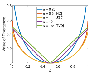
Figure 1: A plot of $D_{f_{\alpha}}$ in (19) for several values of $\alpha$ where $p\sim\text{Ber}(1/2)$ and $q\sim\text{Ber}(\theta)$. Note that HD, JSD, and TVD, are abbreviations for Hellinger, Jensen-Shannon, and Total Variation divergences, respectively. As $\alpha\rightarrow 0$, the curvature of the divergence increases, placing increasingly more weight on $\theta\neq 1/2$. Conversely, for $\alpha\rightarrow\infty$, $D_{f_{\alpha}}$ quickly resembles $D_{f_{\infty}}$, hence a saturation effect of $D_{f_{\alpha}}$.

Remark 1.

It can be inferred from (17) that when the discriminator is trained to optimality, the generator has to minimize the $f_{\alpha}$-divergence hinting at an application of $f$-GAN instead. Implementing $f_{\alpha}$-GAN directly via value function in (5) (for $f_{\alpha}$) involves finding convex conjugate of $f_{\alpha}$, which is challenging in terms of computational complexity making it inconvenient for optimization in the training phase of GANs. In contrast, our approach of using supervised losses circumvents this tedious effort and also provides an operational interpretation of $f_{\alpha}$-divergence via losses. A related work where an $f$-divergence (in particular, $\alpha$-divergence [38]) shows up in the context of GANs, even when the problem formulation is not via $f$-GAN, is by Cai et al. [3]. However, our work differs from [3] in that the value function we use is well motivated via supervised loss functions of binary classification and also recovers the basic GAN [1] (among others).

Remark 2.

As $\alpha\rightarrow 0$, note that (16) implies a more cautious discriminator, i.e., if $p_{G_{\theta}}(x)\geq p_{r}(x)$, then $D_{w^{*}}(x)$ decays more slowly from $1/2$, and if $p_{G_{\theta}}(x)\leq p_{r}(x)$, $D_{w^{*}}(x)$ increases more slowly from $1/2$. Conversely, as $\alpha\rightarrow\infty$, (16) simplifies to $D_{\omega^{*}}(x)=\mathbbm{1}\{p_{r}(x)>p_{G_{\theta}}(x)\}+\frac{1}{2}\mathbbm{1}\{p_{r}(x)=p_{G_{\theta}}(x)\}$, where the discriminator implements the Maximum Likelihood (ML) decision rule, i.e., a hard decision whenever $p_{r}(x)\neq p_{G_{\theta}}(x)$. In other words, (16) for $\alpha\rightarrow\infty$ induces a very confident discriminator. Regarding the generator’s perspective, (17) (and Figure 1) implies that the generator seeks to minimize the discrepancy between $P_{r}$ and $P_{G_{\theta}}$ according to the geometry induced by $D_{f_{\alpha}}$. Thus, the optimization trajectory traversed by the generator during training is strongly dependent on the practitioner’s choice of $\alpha\in(0,\infty]$. Please refer to Figure 2 for an illustration of this observation.

Figure 2: An idealized illustration on the probability simplex of the infimum over $\theta$ in (17) for $\alpha_{1},\alpha_{2}\in(0,\infty]$ such that $\alpha_{1}\neq\alpha_{2}$. The choice of $\alpha$ in the min-max game for the $\alpha$-GAN in (15) defines the optimization trajectory taken by the generator (versus an optimal discriminator as specified in (16)) by distorting the underlying geometry according to $D_{f_{\alpha}}$.

A detailed proof of Theorem 1 is in Appendix A. For intuition on the construction of the function in (18), see Theorem 3. Next we show that $\alpha$-GAN recovers various well known $f$-GANs.

Theorem 2 ($f$-GANs).

$\alpha$-GAN recovers vanilla GAN, Hellinger GAN (H-GAN) [4], and Total Variation GAN (TV-GAN) [4] as $\alpha\rightarrow 1$, $\alpha=\frac{1}{2}$, and $\alpha\rightarrow\infty$, respectively.

A detailed proof is in Appendix B.

IV-A Reconstructing Arimoto Divergence

It is interesting to note that the divergence $D_{f_{\alpha}}(\cdot||\cdot)$ (in (19)) that naturally emerges from the analysis of $\alpha$-GAN was first proposed by Österriecher [22] in the context of statistics and was later referred to as the Arimoto divergence by Liese and Vajda [19]. It was shown to have several desirable properties with applications in statistics and information theory [39, 40]. For example:

• A geometric interpretation of the divergence $D_{f_{\alpha}}$ in the context of hypothesis testing [22].

• $D_{f_{\alpha}}(P||Q)^{\min\{\alpha,\frac{1}{2}\}}$ defines a distance metric (satisfying the triangle inequality) on the set of probability distributions [20].

When the Arimoto divergence $D_{f_{\alpha}}$ was proposed, the convexity of the generating function $f_{\alpha}$ was proved via the traditional second derivative test [22, Lemma 1]. We present an alternative approach to arriving at the Arimoto divergence by utilizing the margin-based form of $\alpha$-loss (see [21]) where the convexity of $f_{\alpha}$ (and also the symmetric property of $D_{f_{\alpha}}(\cdot||\cdot)$) arises in a rather natural manner, thereby reconstructing the Arimoto divergence through a distinct conceptual perspective.

We do this by noticing that the Arimoto divergence falls into the category of a broad class of $f$-divergences that can be obtained from margin-based loss functions. Such a connection between margin-based losses in classification and the corresponding $f$-divergences was introduced by Nguyen et al. [17, Theorem 1]. They observed that, for a given margin-based loss function $\tilde{\ell}$, there is a corresponding $f$-divergence with the convex function $f$ defined as $f(u):=-\inf_{t}\left(u\tilde{\ell}(t)+\tilde{\ell}(-t)\right)$. The convexity of $f$ follows simply because the infimum of affine functions is concave, and this argument does not require $\tilde{\ell}$ to be convex. Additionally, the $f$-divergence obtained is always symmetric because $f$ satisfies $f(u)=uf(\frac{1}{u})$ since $\inf_{t}u\tilde{\ell}(t)+\tilde{\ell}(-t)=\inf_{t}\tilde{\ell}(t)+u\tilde{\ell}(-t)$.

The margin-based $\alpha$-loss [12] for $\alpha\in(0,1)\cup(1,\infty)$, $\tilde{\ell}_{\alpha}:\bar{\mathbb{R}}\rightarrow\mathbb{R}_{+}$ is defined as

$$\tilde{\ell}_{\alpha}(t)\triangleq\frac{\alpha}{\alpha-1}\left(1-{\sigma(t)}^{\frac{\alpha-1}{\alpha}}\right),$$ (20)

where $\sigma:\bar{\mathbb{R}}\rightarrow\mathbb{R}_{+}$ is the sigmoid function given by $\sigma(t)=(1+\mathrm{e}^{-t})^{-1}$. With these preliminaries in hand, we have the following result.

Theorem 3.

For the function $f_{\alpha}$ in (18), it holds that

$$f_{\alpha}(u)=-\inf_{t}\left(u\tilde{\ell}_{\alpha}(t)+\tilde{\ell}_{\alpha}(-t)\right)-\frac{\alpha}{\alpha-1}\left(2^{\frac{1}{\alpha}}-2\right)\\ \text{for}\ u\geq 0.$$ (21)

A detailed proof is in Appendix D.

V Convergence Properties of $\alpha$-GAN

We study convergence properties of $\alpha$-GAN under the assumption of sufficiently large number of samples and discriminator capacity (similar to [23]). Liu et al. [23] addressed a fundamental question in the context of convergence analysis of GANs, in general: For a sequence of generated distributions, does convergence of a divergence between the generated distribution and a fixed real distribution (that the generator wants to minimize) to the global minimum lead to some standard notion of distributional convergence to the real distribution? They answer this question in the affirmative provided $\mathcal{X}$ is a compact metric space. They define adversarial divergences [23, Definition 1] which capture the divergences used by a number of existing GANs that include vanilla GAN [1], $f$-GAN [4], WGAN [5], and MMD-GAN [41]. For strict adversarial divergences (a subclass of the adversarial divergences where the minimizer of the divergence is uniquely the real distribution), they showed that convergence of divergence to global minimum implies weak convergence of the generated distribution to the real distribution. They also obtain a structural result on the class of strict adversarial divergences [23, Corollary 12] based on a notion of relative strength between adversarial divergences.

We first borrow the following terminology from Liu et al. [23] in order to study convergence properties of $\alpha$-GAN: A strict adversarial divergence $\tau_{1}$ is said to be stronger than another adversarial divergence $\tau_{2}$ (or $\tau_{2}$ is said to be weaker than $\tau_{1}$) if for any sequence of probability distributions $(P_{n})$ and target distribution $P$, $\tau_{1}(P\|P_{n})\rightarrow 0$ implies $\tau_{2}(P\|P_{n})\rightarrow 0$. We say $\tau_{1}$ is equivalent to $\tau_{2}$ is $\tau_{1}$ is both stronger and weaker than $\tau_{2}$. We say $\tau_{1}$ is strictly stronger than $\tau_{2}$ if $\tau_{1}$ is stronger than $\tau_{2}$ but not equivalent. We say $\tau_{1}$ and $\tau_{2}$ are not comparable if $\tau_{1}$ is neither stronger nor weaker than $\tau_{2}$.

Arjovsky et al. [5] proved that Jensen-Shannon divergence is equivalent to total variation distance. Later Liu et al. showed that squared Hellinger distance is also equivalent to both these divergences, meaning that all the three divergences belong to the same equivalence class (see [23, Figure 1]). Noticing that squared Hellinger distance, Jensen-Shannon divergence, and total variation distance correspond to Arimoto divergences $D_{f_{\alpha}}(\cdot||\cdot)$ for $\alpha=1/2$, $\alpha=1$, and $\alpha=\infty$, respectively, it is natural to ask the question: Are Arimoto divergences for all $\alpha>0$ equivalent? We answer this question in the affirmative in Theorem 5, thereby adding the Arimoto divergences for all other $\alpha$ also to the same equivalence class. As a motivation for a proof of this, we first give an alternative and more simpler proof for the equivalence of Jensen-Shannon divergence and total variation distance  [5, Theorem 2(1)].

Theorem 4.

The Jensen-Shannon divergence is equivalent to the total variation distance.

Proof.

We first show that the total variation distance is stronger than the Jensen-Shannon divergence. Consider a sequence of probability distributions $(P_{n})$ such that $D_{\text{TV}}(P_{n}||P)\rightarrow 0$. Using the fact that the total variation distance upper bounds the Jensen-Shannon divergence [26, Theorem 3], we have $D_{\text{JS}}(P_{n}||P)\leq(\log{2})D_{\text{TV}}(P_{n}||P)$, for each $n\in\mathbbm{N}$. This implies that $D_{\text{JS}}(P_{n}||P)\rightarrow 0$ since $D_{\text{TV}}(P_{n}||P)\rightarrow 0$. This greatly simplifies the corresponding proof of [5, Theorem 2(1)] which uses measure-theoretic analysis, in particular, the Radon-Nikodym theorem. The proof for the other direction, i.e., the Jensen-Shannon divergence is stronger than the total variation distance, is exactly along the same lines as that of [5, Theorem 2(1)] using triangular and Pinsker’s inequalities. ∎

Theorem 5.

Arimoto divergences for all $\alpha>0$ are equivalent. That is, for a sequence of probability distributions $(P_{n})$, $D_{f_{\alpha_{1}}}(P_{n}||P)\rightarrow 0$ if and only if $D_{f_{\alpha_{2}}}(P_{n}||P)\rightarrow 0$ for any $\alpha_{1}\neq\alpha_{2}$.

A detailed proof is in Appendix C.

VI Conclusion

We have shown that a classical information-theoretic measure (Arimoto divergence) characterizes the ideal performance of a modern machine learning algorithm ($\alpha$-GAN) which interpolates between several canonical GANs. For future work, we will investigate $\alpha$-GAN in practice, with particular interest in its generalization guarantees and its efficacy to reduce mode collapse.

Appendix A Proof of Theorem 1

For a fixed generator, $G_{\theta}$, we first solve the optimization problem

$$\sup_{\omega\in\Omega}\int_{\mathcal{X}}\frac{\alpha}{\alpha-1}\left(p_{r}(x)D_{\omega}(x)^{\frac{\alpha-1}{\alpha}}+p_{G_{\theta}}(x)(1-D_{\omega}(x))^{\frac{\alpha-1}{\alpha}}\right).$$ (22)

Consider the function

$$g(y)=\frac{\alpha}{\alpha-1}\left(ay^{\frac{\alpha-1}{\alpha}}+b(1-y)^{\frac{\alpha-1}{\alpha}}\right),$$ (23)

for $a,b\in\mathbb{R}_{+}$ and $y\in[0,1]$. To show that the optimal discriminator is given by the expression in (16), it suffices to show that $g(y)$ achieves its maximum in $[0,1]$ at $y^{*}=\frac{a^{\alpha}}{a^{\alpha}+b^{\alpha}}$. Notice that for $\alpha>1$, $y^{\frac{\alpha-1}{\alpha}}$ is a concave function of $y$, meaning the function $g$ is concave. For $0<\alpha<1$, $y^{\frac{\alpha-1}{\alpha}}$ is a convex function of $y$, but since $\frac{\alpha}{\alpha-1}$ is negative, the overall function $g$ is again concave. Consider the derivative $g^{\prime}(y^{*})=0$, which gives us

$$y^{*}=\frac{a^{\alpha}}{a^{\alpha}+b^{\alpha}}.$$ (24)

This gives (16). With this, the optimization problem in (15) can be written as $\inf_{\theta\in\Theta}C(G_{\theta})$, where

$$C(G_{\theta})=\frac{\alpha}{\alpha-1}\times$$

$$\left[\int_{\mathcal{X}}\left(p_{r}(x)D_{\omega^{*}}(x)^{\frac{\alpha-1}{\alpha}}+p_{G_{\theta}}(x)(1-D_{\omega^{*}}(x))^{\frac{\alpha-1}{\alpha}}\right)dx-2\right]$$ (25)

$$=\frac{\alpha}{\alpha-1}\Bigg{[}\int_{\mathcal{X}}\Bigg{(}p_{r}(x)\left(\frac{p_{r}(x)^{\alpha}}{p_{r}(x)^{\alpha}+p_{G_{\theta}}(x)^{\alpha}}\right)^{\frac{\alpha-1}{\alpha}}+$$

$$\hskip 12.0ptp_{G_{\theta}}(x)\left(\frac{p_{r}(x)^{\alpha}}{p_{r}(x)^{\alpha}+p_{G_{\theta}}(x)^{\alpha}}\right)^{\frac{\alpha-1}{\alpha}}\Bigg{)}dx-2\Bigg{]}$$ (26)

$$=\frac{\alpha}{\alpha-1}\left(\int_{\mathcal{X}}\left(p_{r}(x)^{\alpha}+p_{G_{\theta}}(x)^{\alpha}\right)^{\frac{1}{\alpha}}dx-2\right)$$ (27)

$$=D_{f_{\alpha}}(P_{r}||P_{G_{\theta}})+\frac{\alpha}{\alpha-1}\left(2^{\frac{1}{\alpha}}-2\right),$$ (28)

where for the convex function $f_{\alpha}$ in (18),

$$D_{f_{\alpha}}(P_{r}||P_{G_{\theta}})=\int_{\mathcal{X}}p_{G_{\theta}}(x)f_{\alpha}\left(\frac{p_{r}(x)}{p_{G_{\theta}}(x)}\right)dx$$ (29)

$$=\frac{\alpha}{\alpha-1}\left(\int_{\mathcal{X}}\left(p_{r}(x)^{\alpha}+p_{G_{\theta}}(x)^{\alpha}\right)^{\frac{1}{\alpha}}dx-2^{\frac{1}{\alpha}}\right).$$ (30)

This gives us (17). Since $D_{f_{\alpha}}(P_{r}||P_{G_{\theta}})\geq 0$ with equality if and only if $P_{r}=P_{G_{\theta}}$, we have $C(G_{\theta})\geq\frac{\alpha}{\alpha-1}\left(2^{\frac{1}{\alpha}}-2\right)$ with equality if and only if $P_{r}=P_{G_{\theta}}$.

Appendix B Proof of Theorem 2

First, using L’Hôpital’s rule we can verify that, for $a,b>0$,

$$\lim_{\alpha\rightarrow 1}\frac{\alpha}{\alpha-1}\left(\left(a^{\alpha}+b^{\alpha}\right)^{\frac{1}{\alpha}}-2^{\frac{1}{\alpha}-1}(a+b)\right)\\ =a\log{\left(\frac{a}{\frac{a+b}{2}}\right)}+b\log{\left(\frac{b}{\frac{a+b}{2}}\right)}.$$ (31)

Using this, we have

$$D_{f_{1}}(P_{r}||P_{G_{\theta}})\triangleq\lim_{\alpha\rightarrow 1}D_{f_{\alpha}}(P_{r}||P_{G_{\theta}})$$ (32)

$$=\lim_{\alpha\rightarrow 1}\frac{\alpha}{\alpha-1}\left(\int_{\mathcal{X}}\left(p_{r}(x)^{\alpha}+p_{G_{\theta}}(x)^{\alpha}\right)^{\frac{1}{\alpha}}dx-2^{\frac{1}{\alpha}}\right)$$ (33)

$$=\lim_{\alpha\rightarrow 1}\Bigg{[}\frac{\alpha}{\alpha-1}\times$$

$$\int_{\mathcal{X}}\left(\left(p_{r}(x)^{\alpha}+p_{G_{\theta}}(x)^{\alpha}\right)^{\frac{1}{\alpha}}-2^{\frac{1}{\alpha}-1}(p_{r}(x)+p_{G_{\theta}}(x))\right)dx\Bigg{]}$$ (34)

$$=\int_{\mathcal{X}}p_{r}(x)\log{\frac{p_{r}(x)}{\left(\frac{p_{r}(x)+p_{G_{\theta}}(x)}{2}\right)}}dx+$$

$$\hskip 12.0pt\int_{\mathcal{X}}p_{G_{\theta}}(x)\log{\frac{p_{G_{\theta}}(x)}{\left(\frac{p_{r}(x)+p_{G_{\theta}}(x)}{2}\right)}}dx$$ (35)

$$=:2D_{\text{JS}}(P_{r}||P_{G_{\theta}}),$$ (36)

where $D_{\text{JS}}(\cdot||\cdot)$ is the Jensen-Shannon divergence. Now, as $\alpha\rightarrow 1$, (17) equals $\inf_{\theta\in\Theta}2D_{\text{JS}}(P_{r}||P_{G_{\theta}})-\log{4}$ recovering vanilla GAN.

Substituting $\alpha=\frac{1}{2}$ in (19), we get

$$D_{f_{\frac{1}{2}}}(P_{r}||P_{G_{\theta}}) =-\int_{\mathcal{X}}\left(\sqrt{p_{r}(x)}+\sqrt{p_{G_{\theta}}(x)}\right)^{2}dx+4$$ (37)

$$=\int_{\mathcal{X}}\left(\sqrt{p_{r}(x)}-\sqrt{p_{G_{\theta}}(x)}\right)^{2}dx$$ (38)

$$=:2D_{\text{H}^{2}}(P_{r}||P_{G_{\theta}}),$$ (39)

where $D_{\text{H}^{2}}(P_{r}||P_{G_{\theta}})$ is the squared Hellinger distance. For $\alpha=\frac{1}{2}$, (17) gives $2\inf_{\theta\in\Theta}D_{\text{H}^{2}}(P_{r}||P_{G_{\theta}})-2$ recovering Hellinger GAN (up to a constant).

Noticing that, for $a,b>0$, $\lim_{\alpha\rightarrow\infty}\left(a^{\alpha}+b^{\alpha}\right)^{\frac{1}{\alpha}}=\max\{a,b\}$ and defining $\mathcal{A}:=\{x\in\mathcal{X}:p_{r}(x)\geq p_{G_{\theta}}(x)\}$, we have

$$D_{f_{1}}(P_{r}||P_{G_{\theta}})\triangleq\lim_{\alpha\rightarrow\infty}D_{f_{\alpha}}(P_{r}||P_{G_{\theta}})$$ (40)

$$=\lim_{\alpha\rightarrow\infty}\frac{\alpha}{\alpha-1}\left(\int_{\mathcal{X}}\left(p_{r}(x)^{\alpha}+p_{G_{\theta}}(x)^{\alpha}\right)^{\frac{1}{\alpha}}dx-2^{\frac{1}{\alpha}}\right)$$ (41)

$$=\int_{\mathcal{X}}\max\{p_{r}(x),p_{G_{\theta}}(x)\}\ dx-1$$ (42)

$$=\int_{\mathcal{X}}\max\{p_{r}(x)-p_{G_{\theta}}(x),0\}\ dx$$ (43)

$$=\int_{\mathcal{A}}(p_{r}(x)-p_{G_{\theta}}(x))\ dx$$ (44)

$$=\int_{\mathcal{A}}\frac{p_{r}(x)-p_{G_{\theta}}(x)}{2}\ dx+\int_{\mathcal{A}^{c}}\frac{p_{G_{\theta}}(x)-p_{r}(x)}{2}\ dx$$ (45)

$$=\frac{1}{2}\int_{\mathcal{X}}\left|p_{r}(x)-p_{G_{\theta}}(x)\right|\ dx$$ (46)

$$=:D_{\text{TV}}(P_{r}||P_{G_{\theta}}),$$ (47)

where $D_{\text{TV}}(P_{r}||P_{G_{\theta}})$ is the total variation distance between $P_{r}$ and $P_{G_{\theta}}$. Thus, as $\alpha\rightarrow\infty$, (17) equals $\inf_{\theta\in\Theta}D_{\text{TV}}(P_{r}||P_{G_{\theta}})-1$ recovering TV-GAN (modulo a constant).

Appendix C Proof of Theorem 5

Consider a sequence of probability distributions $(P_{n})$. To prove the theorem, notice that it suffices to show that Arimoto divergence for any $\alpha>0$ is equivalent to the total variation distance, i.e., $D_{f_{\alpha}}(P_{n}||P)\rightarrow 0$ if and only if $D_{\text{TV}}(P_{n}||P)\rightarrow 0$. To this end, we employ a property of Arimoto divergence which gives lower and upper bounds on it in terms of the total variation distance. In particular, Österreicher and Vajda [20, Theorem 2] proved that for any $\alpha>0$, probability distributions $P$ and $Q$, we have

$$\psi_{\alpha}(D_{\text{TV}}(P||Q))\leq D_{f_{\alpha}}(P||Q)\leq\psi_{\alpha}(1)D_{\text{TV}}(P||Q),$$ (48)

where the function $\psi_{\alpha}:[0,1]\rightarrow\mathcal{R}$ defined by $\psi_{\alpha}(p)=\frac{\alpha}{\alpha-1}\left(\left(\left(1+p\right)^{\alpha}+\left(1-p\right)^{\alpha}\right)^{\frac{1}{\alpha}}-2^{\frac{1}{\alpha}}\right)$ for $\alpha\in(0,1)\cup(1,\infty)$ is convex and strictly monotone increasing such that $\psi_{\alpha}(0)=0$ and $\psi_{\alpha}(1)=\frac{\alpha}{\alpha-1}\left(2-2^{\frac{1}{\alpha}}\right)$.

We first prove the ‘only if’ part, i.e., Arimoto divergence is stronger than the total variation distance. Suppose $D_{f_{\alpha}}(P_{n}||P)\rightarrow 0$. From the lower bound in (48), it follows that $\psi_{\alpha}(D_{\text{TV}}(P_{n}||P))\leq D_{f_{\alpha}}(P_{n}||P)$, for each $n\in\mathbbm{N}$. This implies that $\psi_{\alpha}(D_{\text{TV}}(P_{n}||P))\rightarrow 0$. We show below that $\psi_{\alpha}$ is invertible and $\psi_{\alpha}^{-1}$ is continuous. Then it would follow that $\psi_{\alpha}^{-1}\psi_{\alpha}(D_{\text{TV}}(P_{n}||P))=D_{\text{TV}}(P_{n}||P)\rightarrow\psi_{\alpha}^{-1}(0)=0$ proving that Arimoto divergence is stronger than the total variation distance. It remains to show that $\psi_{\alpha}$ is invertible and $\psi_{\alpha}^{-1}$ is continuous. Invertibility follows directly from the fact that $\psi_{\alpha}$ is strictly monotone increasing function. For the continuity of $\psi_{\alpha}^{-1}$, it suffices to show that $\psi_{\alpha}(C)$ is closed for a closed set $C\subseteq[0,1]$. The closed set $C$ is compact since a closed subset of a compact set ($[0,1]$ in this case) is also compact. Note that convexity of $\psi_{\alpha}$ implies continuity and $\psi_{\alpha}(C)$ is compact since a continuous function of a compact set is also compact. By Heine-Borel theorem, this gives that $\psi_{\alpha}(C)$ is closed (and bounded) as desired.

For the ‘if part’, i.e., to prove that the total variation distance is stronger than Arimoto divergence, consider a sequence of probability distributions $(P_{n})$ such that $D_{\text{TV}}(P_{n}||P)\rightarrow 0$. It follows from the upper bound in $\eqref{eqn:boundsonArimoto}$ that $D_{f_{\alpha}}(P_{n}||P)\leq D_{\text{TV}}(P_{n}||P)$, for each $n\in\mathbbm{N}$. This implies that $D_{f_{\alpha}}(P_{n}||P)\rightarrow 0$ which completes the proof.

Appendix D Proof of Theorem 3

We know from [12, Corollary 1] that for $\eta\in[0,1]$,

$$\inf_{t}\eta\tilde{\ell}_{\alpha}(t)+(1-\eta)\tilde{\ell}_{\alpha}(-t) =\frac{\alpha}{\alpha-1}\left(1-\left(\eta^{\alpha}+(1-\eta)^{\alpha}\right)^{\frac{1}{\alpha}}\right).$$

This implies that

$$\inf_{t}\frac{\eta}{1-\eta}\tilde{\ell}_{\alpha}(t)+\tilde{\ell}_{\alpha}(-t)\\ =\frac{\alpha}{\alpha-1}\left(1+\frac{\eta}{1-\eta}-\left(\left(\frac{\eta}{1-\eta}\right)^{\alpha}+1\right)^{\frac{1}{\alpha}}\right)$$ (49)

Now substituting $u$ for $\frac{\eta}{1-\eta}$ and taking negation in (49), we get

$$-\inf_{t}u\tilde{\ell}_{\alpha}(t)+\tilde{\ell}_{\alpha}(-t)=\frac{\alpha}{\alpha-1}\left(\left(u^{\alpha}+1\right)^{\frac{1}{\alpha}}-(1+u)\right),\\ \text{for}\ u\geq 0$$ (50)

giving us (21).

References

- [1] I. J. Goodfellow, J. Pouget-Abadie, M. Mirza, B. Xu, D. Warde-Farley, S. Ozair, A. Courville, and Y. Bengio, “Generative adversarial nets,” in Proceedings of the 27th International Conference on Neural Information Processing Systems - Volume 2, 2014, p. 2672–2680.
- [2] J. H. Lim and J. C. Ye, “Geometric GAN,” arXiv preprint arXiv:1705.02894, 2017.
- [3] L. Cai, Y. Chen, N. Cai, W. Cheng, and H. Wang, “Utilizing amari-alpha divergence to stabilize the training of generative adversarial networks,” Entropy, vol. 22, no. 4, p. 410, 2020.
- [4] S. Nowozin, B. Cseke, and R. Tomioka, “-GAN: Training generative neural samplers using variational divergence minimization,” in Proceedings of the 30th International Conference on Neural Information Processing Systems, 2016, p. 271–279.
- [5] M. Arjovsky, S. Chintala, and L. Bottou, “Wasserstein generative adversarial networks,” in Proceedings of the 34th International Conference on Machine Learning, vol. 70, 2017, pp. 214–223.
- [6] T. Liang, “How well generative adversarial networks learn distributions,” arXiv preprint arXiv:1811.03179, 2018.
- [7] F. Huszár, “How (not) to train your generative model: Scheduled sampling, likelihood, adversary?” arXiv preprint arXiv:1511.05101, 2015.
- [8] L. Metz, B. Poole, D. Pfau, and J. Sohl-Dickstein, “Unrolled generative adversarial networks,” arXiv preprint arXiv:1611.02163, 2016.
- [9] T. Salimans, I. Goodfellow, W. Zaremba, V. Cheung, A. Radford, and X. Chen, “Improved techniques for training GANs,” arXiv preprint arXiv:1606.03498, 2016.
- [10] M. Arjovsky and L. Bottou, “Towards principled methods for training generative adversarial networks,” arXiv preprint arXiv:1701.04862, 2017.
- [11] I. Gulrajani, F. Ahmed, M. Arjovsky, V. Dumoulin, and A. C. Courville, “Improved training of Wasserstein GANs,” in Advances in Neural Information Processing Systems, vol. 30, 2017.
- [12] T. Sypherd, M. Diaz, L. Sankar, and P. Kairouz, “A tunable loss function for binary classification,” in IEEE International Symposium on Information Theory, 2019, pp. 2479–2483.
- [13] T. Sypherd, M. Diaz, L. Sankar, and G. Dasarathy, “On the -loss landscape in the logistic model,” in IEEE International Symposium on Information Theory, 2020, pp. 2700–2705.
- [14] Y. Freund and R. E. Schapire, “A decision-theoretic generalization of on-line learning and an application to boosting,” Journal of Computer and System Sciences, vol. 55, no. 1, pp. 119 – 139, 1997.
- [15] N. Merhav and M. Feder, “Universal prediction,” IEEE Transactions on Information Theory, vol. 44, no. 6, pp. 2124–2147, 1998.
- [16] T. A. Courtade and R. D. Wesel, “Multiterminal source coding with an entropy-based distortion measure,” in IEEE International Symposium on Information Theory, 2011, pp. 2040–2044.
- [17] X. Nguyen, M. J. Wainwright, and M. I. Jordan, “On surrogate loss functions and f-divergences,” The Annals of Statistics, vol. 37, no. 2, pp. 876–904, 2009.
- [18] P. L. Bartlett, M. I. Jordan, and J. D. Mcauliffe, “Convexity, classification, and risk bounds,” Journal of the American Statistical Association, vol. 101, no. 473, pp. 138–156, 2006.
- [19] F. Liese and I. Vajda, “On divergences and informations in statistics and information theory,” IEEE Transactions on Information Theory, vol. 52, no. 10, pp. 4394–4412, 2006.
- [20] F. Österreicher and I. Vajda, “A new class of metric divergences on probability spaces and its applicability in statistics,” Annals of the Institute of Statistical Mathematics, vol. 55, no. 3, pp. 639–653, 2003.
- [21] T. Sypherd, M. Diaz, J. K. Cava, G. Dasarathy, P. Kairouz, and L. Sankar, “A tunable loss function for robust classification: Calibration, landscape, and generalization,” arXiv preprint arXiv:1906.02314, 2019.
- [22] F. Österreicher, “On a class of perimeter-type distances of probability distributions,” Kybernetika, vol. 32, no. 4, pp. 389–393, 1996.
- [23] S. Liu, O. Bousquet, and K. Chaudhuri, “Approximation and convergence properties of generative adversarial learning,” Advances in Neural Information Processing Systems, vol. 30, 2017.
- [24] S. Arimoto, “Information-theoretical considerations on estimation problems,” Information and control, vol. 19, no. 3, pp. 181–194, 1971.
- [25] J. Liao, O. Kosut, L. Sankar, and F. P. Calmon, “A tunable measure for information leakage,” in 2018 IEEE International Symposium on Information Theory (ISIT). IEEE, 2018, pp. 701–705.
- [26] J. Lin, “Divergence measures based on the shannon entropy,” IEEE Transactions on Information Theory, vol. 37, no. 1, pp. 145–151, 1991.
- [27] A. Rényi, “On measures of entropy and information,” in Proceedings of the Fourth Berkeley Symposium on Mathematical Statistics and Probability, 1961, pp. 547–561.
- [28] I. Csiszár, “Information-type measures of difference of probability distributions and indirect observation,” Studia Scientiarum Mathematicarum Hungarica, vol. 2, pp. 229–318, 1967.
- [29] S. M. Ali and S. D. Silvey, “A general class of coefficients of divergence of one distribution from another,” Journal of the Royal Statistical Society. Series B (Methodological), vol. 28, no. 1, pp. 131–142, 1966.
- [30] X. Nguyen, M. J. Wainwright, and M. I. Jordan, “Estimating divergence functionals and the likelihood ratio by convex risk minimization,” IEEE Transactions on Information Theory, vol. 56, no. 11, pp. 5847–5861, 2010.
- [31] C. Villani, Optimal transport: old and new. Springer Science & Business Media, 2008, vol. 338.
- [32] M. Wiatrak, S. V. Albrecht, and A. Nystrom, “Stabilizing generative adversarial networks: A survey,” arXiv preprint arXiv:1910.00927, 2019.
- [33] S. Arora, R. Ge, Y. Liang, T. Ma, and Y. Zhang, “Generalization and equilibrium in generative adversarial nets (GANs),” in Proceedings of the 34th International Conference on Machine Learning, vol. 70, 2017, pp. 224–232.
- [34] M. D. Reid and R. C. Williamson, “Composite binary losses,” The Journal of Machine Learning Research, vol. 11, pp. 2387–2422, 2010.
- [35] Y. Mroueh, T. Sercu, and V. Goel, “McGan: Mean and covariance feature matching GAN,” in Proceedings of the 34th International Conference on Machine Learning, vol. 70, 2017, pp. 2527–2535.
- [36] Y. Mroueh and T. Sercu, “Fisher GAN,” in Advances in Neural Information Processing Systems, vol. 30, 2017.
- [37] Y. Mroueh, C.-L. Li, T. Sercu, A. Raj, and Y. Cheng, “Sobolev GAN,” arXiv preprint arXiv:1711.04894, 2017.
- [38] S.-i. Amari, -Divergence and -Projection in Statistical Manifold. New York, NY: Springer New York, 1985, pp. 66–103.
- [39] P. Cerone, S. S. Dragomir, and F. Österreicher, “Bound on extended -divergences for a variety of classes,” Kybernetika, vol. 40, no. 6, pp. 745–756, 2004.
- [40] I. Vajda, “On metric divergences of probability measures,” Kybernetika, vol. 45, no. 6, pp. 885–900, 2009.
- [41] G. K. Dziugaite, D. M. Roy, and Z. Ghahramani, “Training generative neural networks via maximum mean discrepancy optimization,” arXiv preprint arXiv:1505.03906, 2015.