Prior-Aware Distribution Estimation for Differential Privacy

Abstract

Joint distribution estimation of a dataset under differential privacy is a fundamental problem for many privacy-focused applications, such as query answering, machine learning tasks and synthetic data generation. In this work, we examine the joint distribution estimation problem given two data points: 1) differentially private answers of a workload computed over private data and 2) a prior empirical distribution from a public dataset. Our goal is to find a new distribution such that estimating the workload using this distribution is as accurate as the differentially private answer, and the relative entropy, or KL divergence, of this distribution is minimized with respect to the prior distribution. We propose an approach based on iterative optimization for solving this problem. An application of our solution won second place in the NIST 2020 Differential Privacy Temporal Map Challenge, Sprint 2.

1 Introduction

Personal information collected as flat tabular data is used in many real world applications, such as medical records, community survey records and web visit records [1, 2, 3]. Releasing these sensitive records to the public enables a variety of scientific research, but introduces risk due to privacy leakage. Differential privacy (DP) is a state-of-the-art technique used to prevent privacy leakage [4]. Releasing a synthetic dataset under differential privacy provides public access to data along with strong privacy guarantees.

A common way to synthesize tabular data under DP is to privately learn the joint distribution by injecting noise according to a DP mechanism, such as the Laplace mechanism. When using the Laplace mechanism, we inject noise to each domain value, which results in extremely high error when the total domain size is large, which is common for datasets with multiple attributes. To mitigate this problem, many probabilistic-graphical-model based solutions are proposed, such as decomposing the joint distribution into a product of multiple small marginal distributions through either a Bayesian [5] or Markov network [6, 7, 8, 9]. Another line of approach is to privately learn the joint distribution through estimation. One example, MWEM [10], updates the joint distribution according to the observed noisy marginal distribution using the multiplicative rule. Another example, PGM [8], learns the joint distribution on a graphical model from a marginal manifold while maximizing the entropy of non-observed distributions. All of these techniques are based on first estimating answers to linear queries under DP and then constructing a synthetic dataset from that.

However, all of these approaches assume no knowledge about the data before learning the joint distribution. Given a sensitive dataset for a specific domain, similar datasets can often be found that have been released publicly in the past. We can treat the empirical joint distribution from the public dataset as a prior for our private joint distribution, which contains more information that can not be learned from the DP answers of a workload.

In this work, we consider the joint distribution estimation problem given a prior distribution and the answers to a linear query workload under DP. Our goal is to find a joint distribution such that the answers to the given workload derived from this distribution are sufficiently accurate, and the relative entropy, or KL divergence, of this distribution with respect to the prior is minimized. We believe this approach can improve the quality of the synthetic dataset sampled from the inferred joint distribution to evaluate more queries accurately even outside the given workload, as long as the prior captures the information precisely that we cannot learn from the DP answers of the given workload.

A similar approach is found in PMWPub [11]. It combines MWEM with public data by initializing the joint distribution with the public distribution and updating it using the multiplicative rule according to the noisy answer of the query selected through exponential mechanism from a fixed query class. The goal for PMWPub is to have a synthetic dataset such that any query from the fixed query class can be evaluated accurately. Unlike PMWPub, our goal is to estimate the joint distribution such that not only the given workload can be evaluated accurately, but also the relative entropy of the new distribution with respect to the prior is low.

Our contributions are as follows:

• We initiate the study of joint distribution estimation given a public prior and DP answers to a workload of linear queries.

• The estimated distribution has two characteristics: 1) it has low $L_{1}$ error with respect to the workload. 2) it has low relative entropy with respect to the prior.

• The estimated distribution is tractable since its support is covered by the support of the public prior, which is derived from a public dataset and is tractable by nature.

• An application of this approach was the second place winning solution in the NIST 2020 Differential Privacy Temporal Map Challenge, Sprint 2 [12].

2 Preliminaries

Data. We consider a flat tabular data $D$ with $m$ attributes and $n$ tuples. The domain for each attribute $A_{i}$ is $\Sigma_{i}$, and the domain for a tuple $t$ in $D$ is $\Sigma=\Sigma_{1}\times\Sigma_{2}\times\ldots\Sigma_{m}$. We assume each attribute domain is a discrete domain . Denote $N$ as the size of domain $\Sigma$. We consider a natural ordering of all the domain values in $\Sigma$ such that $\Sigma=\{v_{1},v_{2},...,v_{N}\}$. We use $h=[h_{1},h_{2},\ldots h_{N}]$ to denote the frequency for each domain value $v_{i}$ in $D$, which is a histogram on the domain $\Sigma$ for $D$. We further denote $x=[x_{1},x_{2},\ldots x_{N}]$ where $x_{i}=h_{i}/n$ as the empirical density distribution of the data $D$. We also use the notation $x(v_{i})$ to refer $x_{i}$.

Workload. A linear query $u$ is a vector of size $N$, such that the answer is given as $u^{T}x$. If $u$ only contains $\{0,1\}$, it asks the empirical probability that a tuple in $D$ satisfies any of the predicates defined by $u$. A workload $W$ of $M$ linear queries is a matrix of size $M\times N$, such that the answer is given as $y=Wx$. We assume $W$ only contains $\{0,1\}$, which means all queries are empirical probability queries for some predicates. A $k$-way marginal query is a workload $W$ such that it asks the marginal probability empirically for some $k$ attributes. Denote $u[i]$ as the $i$-th entry in the vector $u$ and $W[i,j]$ as the entry at $i$-th row and $j$-th column. Denote $W[i,*]$ as the $i$-th row in $W$ and $W[*,j]$ as the $j$-th column in $W$. We use $\left\lVert\cdot\right\rVert_{p}$ as the $L_{p}$ norm. Notice that for a matrix $W$, $\left\lVert W\right\rVert_{1}$ is the max entry and $\left\lVert W\right\rVert_{1,1}$ is the sum of absolute values of all entries.

Differential Privacy. We assume the workload is answered under differential privacy.

Definition 2.1 (Differential Privacy).

A randomized mechanism $M:\Sigma^{*}\rightarrow\mathcal{R}$ satisfies $\epsilon$-differential privacy (DP) if for any neighboring datasets $D$ and $D^{\prime}$ which differ by a single tuple, and every event $O\subseteq\mathcal{R}$, we have:

$$\ln{\frac{P(M(D)\in O)}{P(M(D^{\prime})\in O)}}\leq\epsilon$$

A typical differential private mechanism is Laplace mechanism, which adds Laplace noise to the workload answers with the scale proportional to the global sensitivity that is the maximum change of the workload answers by changing one row in the data [4]. We denote $\tilde{y}$ as the mechanism output about answering $y=Wx$.

Prior Distribution We assume a public dataset with the same domain of the private dataset is available. Usually, the mutual information between the public dataset and the private dataset is not trivial. We consider the empirical density distribution from the public dataset as a prior $p$, which is also a vector of size $N$.

Definition 2.2 (KL Divergence [13]).

Given two distributions $q$ and $p$ on the same domain $\Sigma$, the KL divergence is defined as

$$D_{KL}(q||p)=\sum_{v_{i}\in\Sigma}q(v_{i})\log\frac{q(v_{i})}{p(v_{i})}$$ (1)

. This is also called the relative entropy of $q$ with respect to $p$.

Problem Statement. Given a private dataset $D$ with $n$ tuples and a workload $W$ of queries about $x$, the empirical density distribution of $D$, we assume $W$ is answered by some mechanism that satisfies $\epsilon$-DP, such as Laplace mechanism [4] and HDMM [14], and denote the noisy answer as $\tilde{y}$. We also assume a prior distribution $p$ is given, which is the empirical density distribution from a public dataset. The goal is to find a new distribution $q$ such that the followings are satisfied.

• 1) Estimating $W$ from $q$ is at least as accurate as $\tilde{y}$; i.e., we want to minimize the $L1$ distance between $Wq$ and $\tilde{y}$.

• 2) Given the constraint that the distribution $q$ must minimize the $L_{1}$ distance between $Wq$ and $\tilde{y}$, we want $q$ to be as similar as possible to the prior $p$; i.e., the relative entropy of $q$ with respect to the prior $p$, or KL divergence $D_{KL}(q||p)$, is low, according to the minimum relative entropy principle (MRE) [15, 16, 17, 18]. When $p$ is a uniform prior, minimizing the KL divergence $D_{KL}(q||p)$ is equivalent to the principle of maximum entropy [19].

3 Distribution Estimation

In this work, we consider two sources of information that can help us to estimate the distribution of the private data: the prior distribution $p$ and the noisy answer $\tilde{y}$ of the workload $W$. Since $\tilde{y}$ is derived directly from the private data and the prior $p$ is purely an initial guess, we treat $\tilde{y}$ as the first-class information and $p$ as the second-class information. That is, when we estimate the private distribution $q$, we want $Wq$ to be similar to $\tilde{y}$ as much as possible. If there is nothing more we can learn from the noisy answer $\tilde{y}$, we then learn from the prior $p$.

3.1 Two-stage Optimization

Given two optimization goals for the distribution estimation problem, we divide the optimization into two stages. In the first stage, we aim to find a set of valid distribution $q$ such that the $L_{1}$ distance between $Wq$ and $\tilde{y}$ is minimized. Denote $y^{*}=\operatorname*{arg\,min}_{y}\{\left\lVert y-\tilde{y}\right\rVert_{1}\mid\exists z,\left\lVert z\right\rVert_{1}=1,z\geq 0,Wz=y\}$. We argue that $Wq=y^{*}$ is the sufficient and necessary condition that $\left\lVert Wq-\tilde{y}\right\rVert_{1}$ is minimized.

In the second stage, we minimize the relative entropy of $q$ with respect to the prior $p$ with the constraint that $q$ must satisfy $Wq=y^{*}$, which follows the MRE principle:

$$\min\leavevmode\nobreak\ \sum_{v_{i}\in\Sigma}q(v_{i})\log\frac{q(v_{i})}{p(v_{i})}$$

$$s.t.\leavevmode\nobreak\ Wq=y^{*}$$

$$\sum_{v_{i}\in\Sigma}q(v_{i})=1$$

$$\forall v_{i}\in\Sigma,q(v_{i})\geq 0$$ (2)

and denote $q$ as $q^{*}$ when the minimum is achieved. This is the final estimation of the private distribution.

3.2 Optimization Implementation

The first optimization problem is a linear programming problem, which can be solved efficiently if the size of $z$ is small, which is the domain size of the data $D$. When the domain size is large, we can narrow down the domain of $q$ to the support from the prior $p$, which could be much smaller than the original domain size; i.e., $y^{*}=\operatorname*{arg\,min}_{y}\{\left\lVert y-\tilde{y}\right\rVert_{1}\mid\exists z,\left\lVert z\right\rVert_{1}=1,z\geq 0,\left(\forall v_{i}\in\Sigma,p(v_{i})=0\implies z(v_{i})=0\right),Wz=y\}$.

For the second optimization problem, one can apply the method of Lagrange multipliers to solve:

$$\mathcal{L}(q,\lambda,\mu)=\sum_{v_{i}\in\Sigma}q(v_{i})\log\frac{q(v_{i})}{p(v_{i})}-\lambda^{T}(Wq-y^{*})-\mu(\left\lVert q\right\rVert_{1}-1)$$

where the vector $\lambda$ and $\mu$ are Lagrange multipliers. The optimal solution for the original problem is thus given by the values when $\nabla{\mathcal{L}}=0$. Solving $\nabla{\mathcal{L}}=0$ gives [15]

$$q(v_{i})=p(v_{i})\exp\left[-1-\mu-\lambda^{T}W[*,i]\right]$$ (3)

Since KL divergence is convex and the workload $W$ is linear, the solution is unique ([20], chapter 8). However, it is not clear to have a closed form about $\lambda$ and $\mu$.

In the next section, we propose an iterative optimization approach to achieve both optimization goals, which improves the computational efficiency of solving the linear programming problem and bypasses solving the Lagrange multipliers from the equations.

3.3 Iterative Optimization

We consider merging two optimizations into one:

$$\min\leavevmode\nobreak\ \left\lVert Wq-\tilde{y}\right\rVert_{1}$$

$$s.t.\leavevmode\nobreak\ q\in\underset{z\in\mathcal{S}}{\operatorname*{arg\,min}}\left(\sum_{v_{i}\in\Sigma}z(v_{i})\log\frac{z(v_{i})}{p(v_{i})}\right)$$

$$\mathcal{S}=\{z\mid\left\lVert Wz-\tilde{y}\right\rVert_{1}=\left\lVert Wq-\tilde{y}\right\rVert_{1},$$

$$\qquad\quad\;\;\,\left\lVert z\right\rVert_{1}=1,z\geq 0\}$$ (4)

, which finds the optimal distribution $q^{*}$ such that $\left\lVert Wq^{*}-\tilde{y}\right\rVert_{1}$ is minimized first and then the relative entropy of $q^{*}$ with respect to the prior $p$ is also minimized.

Based on this observation, we consider an iterative approach to find the optimal. At the beginning, we set $q$ as $p$. For each iteration, we select some queries from the workload with $L_{1}$-norm equal to 1 as a partial workload $W_{s}$, with corresponding partial noisy answers $\tilde{y}_{s}$. A typical partial workload $W_{s}$ with $L_{1}$-norm equal to 1 is a marginal query. We then find a new positive answer $y_{s}$ to the partial workload, such that $\left\lVert y_{s}-\tilde{y}_{s}\right\rVert_{1}$ is minimized. The sum of $y_{s}$ should be equal to $1$ if $W_{s}$ covers the entire domain, otherwise it should be within $1$. We then update $q$ according to $W_{s}$ and $y_{s}$ such that the relative entropy of $q$ with respect to the prior $p$ is minimized while we ensure $W_{s}q=y_{s}$. The details of distribution update is defined below. After $q$ is updated, we then move on to the next iteration by treating $q$ as the new prior, until the limit of iterations is met.

Definition 3.1 (Distribution Update Function).

Given a prior $p$, a partial workload $W_{s}$ with $L_{1}$-norm equal to 1 and the corresponding optimal answer $y_{s}$, the function $f$ defined as follows is a distribution such that for each domain value $v_{j}\in\Sigma$ :

$$f(p;W_{s},y_{s})[j]=$$

$$\begin{cases}\frac{p[j]y_{s}[i]}{W_{s}[i,*]^{T}p},&\text{if}\leavevmode\nobreak\ \exists i,W_{s}[i,j]>0\leavevmode\nobreak\ \&\leavevmode\nobreak\ W_{s}[i,*]^{T}p>0\\ \frac{y_{s}[i]}{\left\lVert W_{s}[i,*]\right\rVert_{1}},&\text{if}\leavevmode\nobreak\ \exists i,W_{s}[i,j]>0\leavevmode\nobreak\ \&\leavevmode\nobreak\ W_{s}[i,*]^{T}p=0\\ \frac{p[j](1-\left\lVert y_{s}\right\rVert_{1})}{1-\left\lVert W_{s}p\right\rVert_{1}},&\text{if}\leavevmode\nobreak\ \forall i,W_{s}[i,j]=0\leavevmode\nobreak\ \&\leavevmode\nobreak\ 1-\left\lVert W_{s}p\right\rVert_{1}>0\\ \frac{(1-\left\lVert y_{s}\right\rVert_{1})}{N-\left\lVert W_{s}\right\rVert_{1,1}},&\text{if}\leavevmode\nobreak\ \forall i,W_{s}[i,j]=0\leavevmode\nobreak\ \&\leavevmode\nobreak\ 1-\left\lVert W_{s}p\right\rVert_{1}=0\\ \end{cases}$$

Theorem 3.1 (Least Relative Entropy Update).

Given a prior $p$, a partial workload $W_{s}$ with $L_{1}$-norm equal to 1 and the corresponding optimal answer $y_{s}$, the distribution update function $f(p;W_{s},y_{s})$ finds the distribution that is of minimal relative entropy with respect to the prior $p$.

Algorithm 1 Iterative Distribution Estimation

1:A $M\times N$ workload $W$, the corresponding DP answer $\tilde{y}$ based on a private dataset, the public prior $p$, and an iteration parameter $T$.

2:The estimated distribution $q$ of the underlying private data.

3:function IDE($W$, $\tilde{y}$, $p$, $T$)

4:     $q^{(0)}\leftarrow p$

5:     for $t\leftarrow 1\ldots T$ do

6:         Randomly select a partial workload $W_{s}$ from $W$ such that $\left\lVert W_{s}\right\rVert_{1}=1$.

7:         Let $\tilde{y}_{s}$ be the corresponding answers from $\tilde{y}$ regarding to $W_{s}$.

8:         if $\left\lVert W_{s}\right\rVert_{1,1}=N$ then

9:              $y_{s}\leftarrow\operatorname*{arg\,min}_{\left\lVert y_{s}\right\rVert_{1}=1,y_{s}\geq 0}\{\left\lVert y_{s}-\tilde{y}_{s}\right\rVert_{1}\}$

10:         else

11:              $y_{s}\leftarrow\operatorname*{arg\,min}_{\left\lVert y_{s}\right\rVert_{1}\leq 1,y_{s}\geq 0}\{\left\lVert y_{s}-\tilde{y}_{s}\right\rVert_{1}\}$

12:         end if

13:         $q^{(t)}\leftarrow f(q^{(t-1)};W_{s},y_{s})$ $\triangleright$ See Def 3.1

14:     end for

15:     return $q^{(T)}$.

16:end function

Algorithm 1 illustrates the flow of the iterative approach to find $q^{*}$. After each iteration, we reduce the loss about $\left\lVert Wq-\tilde{y}\right\rVert_{1}$, while the rule of distribution update also keeps the updated distribution to be close to the previous distribution in the sense of relative entropy. After sufficient iterations, the loss $\left\lVert Wq-\tilde{y}\right\rVert_{1}$ of the final distribution should be close to the minimal, and the relative entropy of $q$ with respect to the prior $p$ as $D_{KL}(q||p)$ is low. It is not yet clear how convergent this iterative algorithm is.

To boost the computational efficiency, we can narrow down the domain of $q$ as the support of the public prior $p$ for the algorithm. After the algorithm is finished, we can implicitly extend the distribution of $q$ to the full domain such that $q(v_{i})=0$ if $p(v_{i})=0$.

4 Application

In “2020 Differential Privacy Temporal Map Challenge” [12], an application of our approach was the second place winning solution for the sprint 2. This challenge is basically to generate a synthetic dataset such that its k-way marginals has low error.

Data. The data considered in the contest is a subset of IPUMS American Community Survey data [2] about demographic and financial features for some states across some years. The data about states Ohio and Illinois from 2012-2018 is given as a public dataset. Each row of data includes the geographical and temporal features: PUMA and YEAR, and other 33 additional survey features, such as the biological features, work-related features and financial features. The privacy is at the individual level, and we define individual stability $\Delta$ as the max number of records that is associated with a single individual.

Measurement. The error of the synthetic dataset is measured as follows. Both the synthetic dataset and the ground-truth data are first grouped by the PUMA and YEAR. For each group, we randomly choose two attributes other than PUMA and YEAR, generate the marginal distributions empirically from the synthetic and the ground-truth dataset, and compute the $L_{1}$ distance between two marginal distributions, which ranges from 0 to 2. This is repeated for a fixed number of times for each group, and the error for each group is the average $L_{1}$ distance across repetitions. If the total count of a group differs from the true count by 250, the error of that group will be set to 2 as the bias penalty. The final error is the average of errors from all groups.

4.1 Algorithm

The main idea for our approach is based on “select-measure-reconstruct” [14]. We first select some marginal queries, measure them by Laplace mechanism, and then reconstruct the joint distribution by updating the public prior using Algorithm 1 “Iterative Distribution Estimation”. We define it as a subroutine Prior_Update in Algorithm 2 (see Appendix), as it takes a prior as input and outputs an updated prior. An updated prior can be further updated by calling Prior_Update again. We apply this idea in Algorithm 2. Here we consider grouping the private data $D$ by PUMA and YEAR. Each group is expressed as a triple $(puma,year,h)$, where $h$ is the frequency distribution. At the first round, we re-group the data by STATE, which is inferred from the PUMA attribute, and then apply the subroutine to each STATE partition to update the prior. This is because we believe the joint distributions of all PUMA-YEAR groups in the same STATE are similar, and we have sufficient data to update the prior accurately. The workload chosen for the state-level data is denoted as $W_{S}$. Now we get a new prior for each STATE. Within each STATE, we run this subroutine for each PUMA-YEAR group with the new prior. The workload chosen for the group-level data is denoted as $W_{G}$.

Theorem 4.1.

Algorithm 2 satisfies $\epsilon$-DP.

4.2 Parameter Tuning

We also do a heavy parameter tuning for the contest, especially for the choice of workloads.

Workload $W_{S}$ and $W_{G}$. We only consider marginal queries for our workloads. The goal is to find marginal queries such that after we estimate the distribution based on the DP answers of these marginal queries, the total error of all 2-way marginal queries is low. This problem can be viewed as selecting a strategy workload for the target workload with all 2-way marginals in the framework of HDMM [14]. Unlike HDMM, of which the strategy selection is data independent, we consider a data dependent strategy to select the workload based on the public dataset. Given the public dataset, we compute the pair-wise mutual information [21] for all attributes, and covert it into a graph by adding edges with high mutual information. We then select some cliques from the graph as the workload $W_{S}$ for the state-level data, based on the idea of learning distribution by graphical model [5, 6, 7, 8, 9]. For data of each PUMA-YEAR group, since the data size is much smaller, we cannot learn many high-way marginals accurately, so we assume the correlation between attributes in the prior is accurate and we only need to learn some roots in the graphical model. In practice, we select some one-way marginal queries for the workload $W_{G}$ such that those attributes are approximately independent according to the public dataset.

Iteration parameter $T$. The iteration parameter $T$ should be set as a large number to ensure the iterative distribution estimation converges. In practice, we set $T$ as two times the number of marginal queries in the workload during the contest due to the run-time limit. However, if the code implementation is faster, $T$ should be set larger.

4.3 Result

In the contest, the final evaluation is based on a secret dataset that is not publicly accessible. We evaluate our algorithm locally on a private dataset that is the same as the public dataset. Notice that the algorithm doesn’t know that they are the same. Figure 1 shows the average $L_{1}$ error of random 50 2-way marginals for each PUMA-YEAR group under $\epsilon=10$, which is around 0.2 to 0.4. There is also no bias penalty for the synthetic dataset. The result is based on one run of the algorithm.

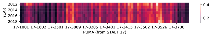
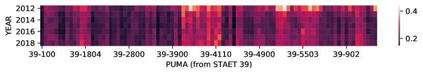
Figure 1: Average L1 error of random 50 2-way marginals for each PUMA-YEAR group under $\epsilon=10$.

Appendix A Algorithms

Algorithm 2 Synthetic Data Generation

1:A workload $W_{S}$ for the state-level data, a workload $W_{G}$ for the group-level data, the private data $D$ as a set of $\{(puma,year,h)\}$ where $h$ is the frequency distribution for the group $(puma,year)$, the public prior $p$, the individual stability $\Delta$, the privacy budget $\epsilon$, and an iteration parameter $T$.

2:A synthetic dataset.

3:function Prior_Update($W,h,p,T,\epsilon_{0}$)

4:     $\tilde{n}\leftarrow\left\lVert h\right\rVert_{1}+Laplace(\Delta/\epsilon_{0})$

5:     $\tilde{n}\leftarrow\lfloor\max\{\tilde{n},0\}\rceil$

6:     $\tilde{y}\leftarrow Wh+Laplace(\left\lVert W\right\rVert_{1}\Delta/\epsilon_{0})$

7:     $\tilde{y}\leftarrow\tilde{y}/\tilde{n}$

8:     $p^{\prime}\leftarrow$ IDE($W,\tilde{y},p,T$) $\triangleright$ See Algorithm 1

9:     return $p^{\prime}$, $\tilde{n}$

10:end function

11:$D^{\prime}\leftarrow\emptyset$

12:$\epsilon_{0}\leftarrow\epsilon/4$

13:for $S\leftarrow$ GROUP-BY($D$, STATE) do

14:     $h_{s}\leftarrow\sum_{(puma,year,h)\in S}h$

15:     $p_{s},\tilde{n}_{s}\leftarrow$ Prior_Update($W_{S},h_{s},p,T,\epsilon_{0}$)

16:     for $(puma,year,h_{g})\in S$ do

17:         $p_{g},\tilde{n}_{g}\leftarrow$ Prior_Update($W_{G},h_{g},p_{s},T,\epsilon_{0}$)

18:         $h^{\prime}\leftarrow$ sample $\tilde{n}_{g}$ tuples from $p_{g}$

19:         $D^{\prime}\leftarrow D^{\prime}\cup(puma,year,h^{\prime})$

20:     end for

21:end for

22:return $D^{\prime}$.

Appendix B Theorem Proof

See 3.1

Proof.

(sketch) Consider the value of $q(v_{i})$ in the optimal solution. For a partial workload $W_{s}$ with $L1$-norm equal to 1, the optimal solution according to the Lagrange function has a simple form:

$$q(v_{i})=p(v_{i})\exp\left[-1-\mu-\lambda_{j}\right]$$

for some $j$ such that $W_{s}[j,i]=1$. We discuss the case latter when there is no $j$ such that this condition holds. Now we fix $j$, from the constraints we have

$$\sum_{i\mid W_{s}[j,i]=1}q(v_{i})=y_{s}[j]$$

. Together we have

$$\sum_{i\mid W_{s}[j,i]=1}p(v_{i})\exp\left[-1-\mu-\lambda_{j}\right]=y_{s}[j]$$

, which implies

$$\exp\left[-1-\mu-\lambda_{j}\right]=\frac{y_{s}[j]}{\sum_{i\mid W_{s}[j,i]=1}p(v_{i})}$$

. Take this back to the first equation, we have

$$q(v_{i})=p(v_{i})\frac{y_{s}[j]}{\sum_{i\mid W_{s}[j,i]=1}p(v_{i})}$$

When $\sum_{i\mid W_{s}[j,i]=1}p(v_{i})=0$, we divide $y_{s}[j]$ equally for each $q(v_{i})$.

For $q(v_{i})$ in the case that there is no $j$ such that $W_{s}[j,i]=1$, the optimal solution has this form:

$$q(v_{i})=p(v_{i})\exp\left[-1-\mu\right]$$

Similar analysis can be applied to this case. Notice that in this case, from the constraints we know that the sum of all such $q(v_{i})$ should be equal to $1-\left\lVert y_{s}\right\rVert_{1}$. ∎

See 4.1

Proof.

(sketch) Each call of Prior_Update runs two Laplace mechanisms sequentially, each satisfy $\epsilon_{0}$-DP. For each PUMA-YEAR group, it is taken (partially) as the input for Prior_Update twice. According to sequential composition rule and parallel composition rule, the entire algorithm satisfies $4\epsilon_{0}$-DP, which is also $\epsilon$-DP. ∎

References

- [1] Fida Kamal Dankar and Khaled El Emam. Practicing differential privacy in health care: A review. Trans. Data Priv., 6(1):35–67, 2013.
- [2] Steven Ruggles, Sarah Flood, Ronald Goeken, Josiah Grover, Erin Meyer, Jose Pacas, and Matthew Sobek. Ipums usa: Version 11.0 [dataset]. Minneapolis, MN: IPUMS, 2021. https://doi.org/10.18128/D010.V11.0.
- [3] Liyue Fan, Luca Bonomi, Li Xiong, and Vaidy Sunderam. Monitoring web browsing behavior with differential privacy. In Proceedings of the 23rd international conference on World wide web, pages 177–188, 2014.
- [4] Cynthia Dwork, Frank McSherry, Kobbi Nissim, and Adam Smith. Calibrating noise to sensitivity in private data analysis. In Theory of cryptography conference, pages 265–284. Springer, 2006.
- [5] Jun Zhang, Graham Cormode, Cecilia M Procopiuc, Divesh Srivastava, and Xiaokui Xiao. Privbayes: Private data release via bayesian networks. ACM Transactions on Database Systems (TODS), 42(4):1–41, 2017.
- [6] Rui Chen, Qian Xiao, Yu Zhang, and Jianliang Xu. Differentially private high-dimensional data publication via sampling-based inference. In Proceedings of the 21th ACM SIGKDD international conference on knowledge discovery and data mining, pages 129–138, 2015.
- [7] Garrett Bernstein, Ryan McKenna, Tao Sun, Daniel Sheldon, Michael Hay, and Gerome Miklau. Differentially private learning of undirected graphical models using collective graphical models. In International Conference on Machine Learning, pages 478–487. PMLR, 2017.
- [8] Ryan McKenna, Daniel Sheldon, and Gerome Miklau. Graphical-model based estimation and inference for differential privacy. In International Conference on Machine Learning, pages 4435–4444. PMLR, 2019.
- [9] Huanyu Zhang, Gautam Kamath, Janardhan Kulkarni, and Steven Wu. Privately learning markov random fields. In International Conference on Machine Learning, pages 11129–11140. PMLR, 2020.
- [10] Moritz Hardt, Katrina Ligett, and Frank McSherry. A simple and practical algorithm for differentially private data release. arXiv preprint arXiv:1012.4763, 2010.
- [11] Terrance Liu, Giuseppe Vietri, Thomas Steinke, Jonathan Ullman, and Zhiwei Steven Wu. Leveraging public data for practical private query release. arXiv preprint arXiv:2102.08598, 2021.
- [12] 2020 differential privacy temporal map challenge. https://www.nist.gov/ctl/pscr/open-innovation-prize-challenges/current-and-upcoming-prize-challenges/2020-differential.
- [13] Solomon Kullback. Information theory and statistics. Courier Corporation, 1997.
- [14] Ryan McKenna, Gerome Miklau, Michael Hay, and Ashwin Machanavajjhala. Optimizing error of high-dimensional statistical queries under differential privacy. arXiv preprint arXiv:1808.03537, 2018.
- [15] Allan D Woodbury and Tadeusz J Ulrych. Minimum relative entropy: Forward probabilistic modeling. Water Resources Research, 29(8):2847–2860, 1993.
- [16] Stefano Olivares and Matteo GA Paris. Quantum estimation via the minimum kullback entropy principle. Physical Review A, 76(4):042120, 2007.
- [17] Zhangshuan Hou and Yoram Rubin. On minimum relative entropy concepts and prior compatibility issues in vadose zone inverse and forward modeling. Water Resources Research, 41(12), 2005.
- [18] Heinz Mühlenbein and Robin Höns. The estimation of distributions and the minimum relative entropy principle. Evolutionary Computation, 13(1):1–27, 2005.
- [19] Edwin T Jaynes. Information theory and statistical mechanics. Physical review, 106(4):620, 1957.
- [20] Jagat Narain Kapur. Maximum-entropy models in science and engineering. John Wiley & Sons, 1989.
- [21] Ralf Steuer, Jürgen Kurths, Carsten O Daub, Janko Weise, and Joachim Selbig. The mutual information: detecting and evaluating dependencies between variables. Bioinformatics, 18(suppl_2):S231–S240, 2002.