Gaussian Mixture Estimation
from Weighted Samples

Abstract

We consider estimating the parameters of a Gaussian mixture density with a given number of components best representing a given set of weighted samples. We adopt a density interpretation of the samples by viewing them as a discrete Dirac mixture density over a continuous domain with weighted components. Hence, Gaussian mixture fitting is viewed as density re-approximation. In order to speed up computation, an expectation–maximization method is proposed that properly considers not only the sample locations, but also the corresponding weights. It is shown that methods from literature do not treat the weights correctly, resulting in wrong estimates. This is demonstrated with simple counterexamples. The proposed method works in any number of dimensions with the same computational load as standard Gaussian mixture estimators for unweighted samples.

TOA short=TOA, long=time of arrival, long-plural-form=times of arrival TDOA short=TDOA, long=time difference of arrival, long-plural-form=time differences of arrival DOTA short=DOTA, long=difference of times of arrival, long-plural-form=differences of times of arrival, short-plural-form=DOTAs ROTA short=ROTA, long=round trip time of arrival, long-plural-form=round trip times of arrival LTDOA short=L-TDOA, long=local time difference of arrival, long-plural-form=local time differences of arrival LDOTA short=L-DOTA, long=local differences of times of arrival, long-plural-form=local differences of times of arrival DOTD short=DOTD, long=difference of time differences TTT short=TTT, long=target transmission time TDOT short=TDOT, long=time difference of transmissions, long-plural-form=time difference of transmissions SSR short=SSR, long=secondary surveillance radar PSR short=PSR, long=primary surveillance radar LORAN short=LORAN, long=long range navigation system MLAT short=MLAT, long=multilateration MLE short=MLE, long=maximum likelihood estimator RSS short=RSS, long=received signal strength AOA short=AOA, long=angle of arrival ML short=ML, long=maximum likelihood MAP short=MAP, long=maximum a posteriori MMSE short=MMSE, long=minimum mean square error RMSE short=RMSE, long=root mean square error LS short=LS, long=least squares LM short=LM, long=Levenberg-Marquardt GNSS short=GNSS, long=global navigation satellite systems GPS short=GPS, long=Global Positioning System ADSB short=ADS-B, long=automatic dependent surveillance – broadcast TOF short=TOF, long=time of flight LORAWAN short=LoRaWAN, long=Long Range Wide Area Network 3DUSCT short=3D-USCT, long=3D-Ultrasound Computer Tomography EKF short=EKF, long=Extended Kalman Filter UKF short=UKF, long=Unscented Kalman Filter SDR short=SDR, long=software–defined radio CPU short=CPU, long=central processing unit CRLB short=CRLB, long=Cramér–Rao lower bound VR short=VR, long=virtual reality SME short=SME, long=Symmetric Measurement Equation LCD short=LCD, long=Localized Cumulative Distribution EM short=EM, long=expectation–maximization S2KF short=S²KF, long=Smart Sampling Kalman Filter ODE short=ODE, long=ordinary differential equation GM short=GM, long=Gaussian mixture DM short=DM, long=Dirac mixture LRKF short=LRKF, long=linear regression Kalman filter CoDiCo short=CoDiCo, long=coupled discrete and continuous densities vMF short=vMF, long=von Mises–Fisher DMD short=DMD, long=Dirac mixture density PDF short=PDF, long=probability density function CDF short=CDF, long=cumulative density function PCD short=PCD, long=projected cumulative distribution

1 Introduction

Gaussian mixture (GM) GM estimation is ubiquitous in signal processing and machine learning. Given a set of samples, the parameters of a GM are determined in such a way as to best fit the samples in a maximum likelihood way. Solutions for equally weighted samples are readily available, EM based methods being the most prevalent because of low computational requirements and ease of implementation.

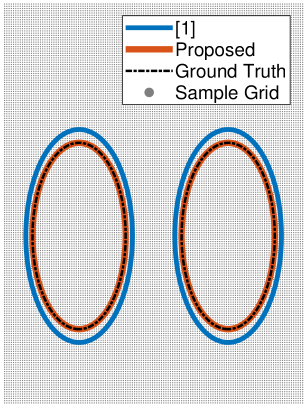
So it comes as a surprise that GM estimation for weighted samples is hard to find in literature. It might be even more surprising that the standard reference Gebru16 gives incorrect results, see Fig. 1.

(a) “separated” components

(b) “overlapping” components

Figure 1: Two-dimensional GM parameter estimation using EM from Gebru16 (blue line), and EM according to our proposed method (red line). Compare the ground truth (black line). Equidistant samples (grey dots) were weighted with the GM density function and given to the EM algorithms.

2 Context

Applications for sample-to-density function approximation include clustering of unlabled data jain1999 ; larsen2002 , multi-target tracking Prembida06 ; Clark2007 , group tracking Pang2011 , multilateration Tzoreff2017 ; Li2018 , and arbitrary density representation in nonlinear filters Dovera2011 ; FUSION20_Frisch .

A popular basic solution to this is the $k$-means algorithm. It does not find a complete density representation, only the means of the individual clusters. The $k$-means algorithm uses hard sample-to-mean associations, therefore yields merely approximate solutions but can be computationally optimized using $k$-d trees Kanungo2002 ; Hamerly2002 . Moreover, the global optimum can be found deterministically Likas2003 , therefore it can be used to provide an initial guess for more elaborate algorithms.

A sample-to-density approximation that is optimal in a maximum likelihood sense can be searched with numerical optimization techniques such as the Newton algorithm that has quadratic convergence but high computational demand per iteration, quasi-Newton methods, the method of scoring, or the conjugate gradient method with slower convergence but less computational effort per iteration Redner84_EM .

2.1 State-of-the-art

The EM algorithm has been used for decades Dempster77 ; wu83_EM to solve statistical problems. It converges rather slowly, especially if the GM components are poorly separated, but it provides a valid parameter set in every iteration step, i.e., nonnegative and normalized component weights and positive semidefinite covariance matrices, without the need of any artificial safeguards. The EM algorithm features good global convergence to some local optimum, is very easy to implement, has low computational cost per iteration when using optimized libraries for standard statistical tasks, and needs little storage Redner84_EM . There are extensions of the EM to automatically determine the optimal number of Gaussian components Figueiredo2002 ; Zhang2004 ; Melynkov2012 .

2.2 Contribution

The contribution of this paper is a fast, simple, and practical EM method for the correct treatment of weighted samples in Gaussian mixture estimation.

3 Problem Formulation

For an observed set of $L$ weighted samples

$${{\mathbf{Y}}}=\left\{\left\{{\alpha}_{1},{\underline{s}}_{1}\right\},\left\{{\alpha}_{2},{\underline{s}}_{2}\right\},\ldots,\left\{{\alpha}_{L},{\underline{s}}_{L}\right\}\right\}$$

with sample locations ${\underline{s}}_{i}$ as vectors in the $D$-dimensional Euclidean space $\mathbb{R}^{D}$, and scalar weights ${\alpha}_{i}$, we want to find a GM density function with $M$ Gaussian components

$$f({\underline{x}}|{{\mathbf{\Theta}}}) =\sum_{m=1}^{M}{w}_{m}\,{\cal N}\!\left({\underline{x}}-{\underline{\mu}}_{m},\;{{\mathbf{C}}}_{m}\right)\enspace,$$ (1)

$${\cal N}\!\left({\underline{x}}-{\underline{\mu}},\;{{\mathbf{C}}}\right) =\frac{\exp\!\left\{-\frac{1}{2}\left({\underline{x}}-{\underline{\mu}}\right)^{\top}\!{{\mathbf{C}}}^{-1}\left({\underline{x}}-{\underline{\mu}}\right)\right\}}{\sqrt{\left|2\pi{{\mathbf{C}}}\right|}}\enspace,$$ (2)

with nonnegative component weights ${w}_{m}\geq 0$ that are normalized, $\sum_{m=1}^{M}{w}_{m}=1$, component means ${\underline{\mu}}_{m}\in\mathbb{R}^{D}$, and component covariances ${{\mathbf{C}}}_{m}\in\mathbb{R}^{D\times D}$. The GM should explain the observed samples as good as possible. We thus estimate GM parameters ${{\mathbf{\Theta}}}$

$${{\mathbf{\Theta}}} =\left\{\left\{{w}_{1},{\underline{\mu}}_{1},{{\mathbf{C}}}_{1}\right\},\;\ldots,\;\left\{{w}_{M},{\underline{\mu}}_{M},{{\mathbf{C}}}_{M}\right\}\right\}$$ (3)

from the weighted samples ${{\mathbf{Y}}}$, ideally in a maximum likelihood sense

$$\widehat{{\mathbf{\Theta}}} =\operatorname*{arg\,max}_{{\mathbf{\Theta}}}\left\{f_{{{{\mathbf{Y}}}|{{\mathbf{\Theta}}}}}^{\!}({{\mathbf{Y}}}\,|\,{{\mathbf{\Theta}}})\right\}\enspace.$$ (4)

This can be done via numerical optimization or, more efficiently, using the EM algorithm. For the EM algorithm, we additionally consider a hidden variable ${{\mathbf{H}}}$. It contains the association probabilities $\eta_{i,m}$ between samples $\left\{{\alpha}_{i},{\underline{s}}_{i}\right\}$ and GM components $\left\{{w}_{m},{\underline{\mu}}_{m},{{\mathbf{C}}}_{m}\right\}\,$.

4 Key Idea

We believe that the following two things should give the same contribution to the result: First, one sample with double weight, and second, two single-weight samples that are arranged with infinitesimally small or zero distance. Therefore, we propose to determine the hidden association parameters ${{\mathbf{H}}}$ only based on sample locations. In other words we use the observed sample weights only in the maximization step and not in the expectation step.

For the maximization step, we propose to estimate GM component weights, means, and covariances as a weighted average, where weighting is the product of observed sample weights and sample-to-GM component associations.

5 Implementation of Proposed Method

Associations ${{\mathbf{H}}}$ between Samples and GM components are unknown but necessary for an EM algorithm in order to independently calculate moments of individual mixtures. Marginalization over all possible associations

$$f_{{{{\mathbf{Y}}}|{{\mathbf{\Theta}}}}}^{\!}({{\mathbf{Y}}}|{{\mathbf{\Theta}}}) =\int f_{{{{\mathbf{H}}},{{\mathbf{Y}}}|{{\mathbf{\Theta}}}}}^{\!}({{\mathbf{H}}},{{\mathbf{Y}}}\,|\,{{\mathbf{\Theta}}}){\,\operatorfont{d}}{{\mathbf{H}}}\enspace,$$ (5)

is infeasible, hence the separation into expectation and maximization steps according to the EM algorithm.

5.1 Expectation Step

Besides the given observed data ${{\mathbf{Y}}}$, we assume an estimate ${\widehat{{\mathbf{\Theta}}}^{(r)}}$ of the parameter vector containing the GM parameters $\left\{{w}_{m}^{(r)},{\underline{\mu}}_{m}^{(r)},{{\mathbf{C}}}_{m}^{(r)}\right\}\,$,  $m\in\left\{1,\ldots,M\right\}$, with iteration index $(r)$, to obtain a new estimate of the hidden data ${\widehat{{\mathbf{H}}}^{(r+1)}}$

$$\eta_{i,m}^{(r+1)}=\frac{{w}_{m}\,{\cal N}\!\left({\underline{s}}_{i}-{\underline{\mu}}_{m}^{(r)},\;{{\mathbf{C}}}_{m}^{(r)}\right)}{\sum_{\widetilde{m}=1}^{M}{w}_{\widetilde{m}}\,{\cal N}\!\left({\underline{s}}_{i}-{\underline{\mu}}_{\widetilde{m}}^{(r)},\;{{\mathbf{C}}}_{\widetilde{m}}^{(r)}\right)}\enspace,$$ (6)

with matrix elements $\left[{\widehat{{\mathbf{H}}}^{(r+1)}}\right]_{i,m}\!=\eta_{i,m}^{(r+1)}$. Due to the normalization such that the row sum is equal to one, ${\widehat{{\mathbf{H}}}^{(r+1)}}$ describes a “probability of association” for each sample $i$ to each component $m$ of the GM.

5.2 Maximization Step

Using said estimate of the hidden data ${\widehat{{\mathbf{H}}}^{(r+1)}}$ and also the observed data ${{\mathbf{Y}}}$, i.e., sample locations ${\underline{s}}_{i}$ and sample weights ${\alpha}_{i}$, we obtain a new estimate of the parameter vector ${\widehat{{\mathbf{\Theta}}}^{(r+1)}}$

$${w}_{m}^{(r+1)} =\frac{\sum_{i=1}^{L}\eta_{i,m}^{(r+1)}{\alpha}_{i}}{\sum_{\widetilde{m}=1}^{M}\sum_{\tilde{i}=1}^{L}\eta_{\tilde{i},\widetilde{m}}^{(r+1)}{\alpha}_{\tilde{i}}}\enspace,$$ (7)

$${\underline{\mu}}_{m}^{(r+1)} =\frac{\sum_{i=1}^{L}\eta_{i,m}^{(r+1)}{\alpha}_{i}\,{\underline{s}}_{i}}{\sum_{\tilde{i}=1}^{L}\eta_{\tilde{i},m}^{(r+1)}{\alpha}_{\tilde{i}}}\enspace,$$ (8)

$${{\mathbf{C}}}_{m}^{(r+1)} =\frac{\sum_{i=1}^{L}\eta_{i,m}^{(r+1)}{\alpha}_{i}\left({\underline{s}}_{i}-{\underline{\mu}}_{m}^{(r+1)}\right)\left({\underline{s}}_{i}-{\underline{\mu}}_{m}^{(r+1)}\right)^{\top}}{\sum_{\tilde{i}=1}^{L}\eta_{\tilde{i},m}^{(r+1)}{\alpha}_{\tilde{i}}}\enspace.$$ (9)

(d) Weights; “overlapping” components

(e) Means; “overlapping” components

(f) Standard deviations; “overlapping” components

(g) Densities; “separated” components

(h) Densities; “overlapping” components

Figure 2: A simple scalar example with two GM components. Equidistant samples were weighted with the ground truth probability density function, and the GM parameters (component weights, means, and variances) were estimated with our proposed method (red lines) and the method from Gebru16 (blue lines). Ideally, the estimations should converge to the ground truth (black dashed lines) after some iterations.

5.3 Split Sample Linearity

The obtained parameter estimate ${\widehat{{\mathbf{\Theta}}}^{(r+1)}}$, after performing one expectation and maximization step for some given prior parameter estimate ${\widehat{{\mathbf{\Theta}}}^{(r)}}$, is identical whether we have a set of weighted samples

$${{\mathbf{Y}}}=\left\{\left\{{\alpha}_{1},{\underline{s}}_{1}\right\},\left\{{\alpha}_{2},{\underline{s}}_{2}\right\},\ldots,\left\{{\alpha}_{L},{\underline{s}}_{L}\right\}\right\}\;,$$

or “split samples” with, e.g., two samples and two weights at each sample location, i.e.,

$$\widetilde{{\mathbf{Y}}}= \bigg{\{}\left\{{\alpha}_{1}^{(1)}\!,\,{\underline{s}}_{1}\right\},\left\{{\alpha}_{1}^{(2)}\!,\,{\underline{s}}_{1}\right\},\;\left\{{\alpha}_{2}^{(1)}\!,\,{\underline{s}}_{2}\right\},\left\{{\alpha}_{2}^{(2)}\!,\,{\underline{s}}_{2}\right\},$$ (10)

$$\quad\ldots,\;\left\{{\alpha}_{L}^{(1)}\!,\,{\underline{s}}_{L}\right\},\left\{{\alpha}_{L}^{(2)}\!,\,{\underline{s}}_{L}\right\}\bigg{\}}\enspace,$$ (11)

with ${\alpha}_{i}={\alpha}_{i}^{(1)}+{\alpha}_{i}^{(2)}\;\forall\;i\in\left\{1,\ldots,L\right\}$. This is because association probabilities $\eta_{i,m}^{(r+1)}$ in the expectation step do not depend on sample weights ${\alpha}_{i}$, and for the maximization step due to its linearity it does not matter whether there are two samples with weights ${\alpha}_{i}^{(1)}\!,\,{\alpha}_{i}^{(2)}$ at the same location ${\underline{s}}_{i}\,$, or only one sample that contains their combined weight ${\alpha}_{i}$.

Note that the same holds for any other linear combination of more than two weights and samples at each same sample location, moreover not all but only a few sample locations may exhibit “split samples”. We see this invariance against “split samples” as a logical sanity check the method should pass in order to be consistent.

6 Implementation in Gebru16

For comparison, we quote the implementation from Gebru16 ; Gebru14 and highlight the differences to what we propose.

6.1 Expectation Step in Gebru16

For estimating the associations $\eta_{i,m}^{(r+1)}$ between samples ${\underline{s}}_{i}$ and GM components $\left\{{w}_{m}^{(r)},{\underline{\mu}}_{m}^{(r)},{{\mathbf{C}}}_{m}^{(r)}\right\}$, the covariances ${{\mathbf{C}}}_{m}^{(r)}$ of the individual Gaussian components are scaled in Gebru16 based on the sample weights ${\alpha}_{i}$

$$\eta_{i,m}^{(r+1)}=\frac{{w}_{m}\,{\cal N}\!\left({\underline{s}}_{i}-{\underline{\mu}}_{m}^{(r)},\;{{\mathbf{C}}}_{m}^{(r)}/{\alpha}_{i}\right)}{\sum_{\widetilde{m}=1}^{M}{w}_{\widetilde{m}}\,{\cal N}\!\left({\underline{s}}_{i}-{\underline{\mu}}_{\widetilde{m}}^{(r)},\;{{\mathbf{C}}}_{\widetilde{m}}^{(r)}/{\alpha}_{i}\right)}\enspace.$$ (12)

We however propose to use the GM covariances ${{\mathbf{C}}}_{m}^{(r)}$ without any sample-specific adaptions (6).

6.2 Maximization Step in Gebru16

In Gebru16 , sample weights ${\alpha}_{i}$ are not considered when calculating the Gaussian mixture component weights ${w}_{m}^{(r+1)}$

$${w}_{m}^{(r+1)} =\frac{1}{L}\sum_{i=1}^{L}\eta_{i,m}^{(r+1)}\enspace,$$ (13)

compare (7). Calculation of component means ${\underline{\mu}}_{m}^{(r+1)}$

$${\underline{\mu}}_{m}^{(r+1)} =\frac{\sum_{i=1}^{L}\eta_{i,m}^{(r+1)}{\alpha}_{i}{\underline{s}}_{i}}{\sum_{\tilde{i}=1}^{L}\eta_{\tilde{i},m}^{(r+1)}{\alpha}_{\tilde{i}}}$$ (14)

is identical to our proposed method (8). For component covariance estimation ${{\mathbf{C}}}_{m}^{(r+1)}$, the difference between Gebru16 and our proposed method (9) is that sample weights ${\alpha}_{i}$ are not considered for normalization

$${{\mathbf{C}}}_{m}^{(r+1)} =\frac{\sum_{i=1}^{L}\eta_{i,m}^{(r+1)}{\alpha}_{i}\left({\underline{s}}_{i}-{\underline{\mu}}_{m}^{(r+1)}\right)\left({\underline{s}}_{i}-{\underline{\mu}}_{m}^{(r+1)}\right)^{\top}}{\sum_{\tilde{i}=1}^{L}\eta_{\tilde{i},m}^{(r+1)}}\enspace.$$ (15)

6.3 Split Sample Linearity in Gebru16

For the EM method according to Gebru16 , the result of each iteration is different when we “split” some samples in different ways, e.g., in two parts (11). Therefore, a double sample weight is not equivalent with two samples at the same location. The evaluation section will demonstrate that not only the individual iteration results, but also the final result differs from our proposed method, and from the ground truth.

7 Evaluation and Comparison with Gebru16

As the simplest example, we define a one-dimensional GM with two components. A large number of equidistant samples is placed in the relevant region, and the GM density function at each sample location is used as the respective sample weight. Furthermore, some random initial guess of the GM parameters is given. Two algorithms are compared in solving this density estimation problem. First, our proposed method as defined in Sec. 5, and second, the method as proposed in Gebru16 and replicated here in Sec. 6.

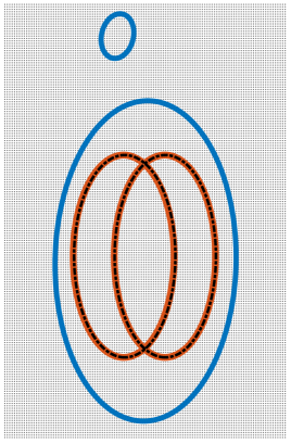
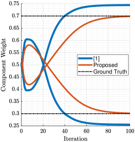
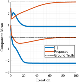
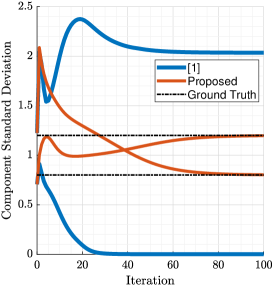
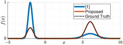
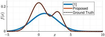
One setup is defined where the two Gaussian components are rather “separated”, this can be solved with about 15 iteration steps, see Fig. 5.2 (a, b, c). A second setup has Gaussian components that are closer together and exhibit some “overlap” of probability mass. Both EM algorithms need much more iteration steps to converge here, see Fig. 5.2 (d, e, f).

For the “separated” Gaussian components we find that all algorithms provide a very good estimation of the GM component means after about three iterations. The weighting factor estimates need more iterations to converge and are slightly off with the algorithm from Gebru16 . Standard deviations from Gebru16 are not reliable at all. Only our proposed method provides accurate results here. In the “overlapping” setup, the GM component weight, mean, and variance estimates converge to solutions that are significantly off the ground truth when using the method from Gebru16 . Our proposed method needs more iterations to converge but finds the accurate solution in the end.

8 Conclusions

Considering weighted samples opens new applications for GM estimation, e.g., in the field of Bayesian estimation, see FUSION20_Frisch . The correct treatment of weighted samples in GM estimation was derived. It was shown that current approaches have a serious flaw that leads to wrong estimates. The proper modifications can simply be added to existing GM estimation code to extend its applicability to weighted samples. The proposed method is also a plugin replacement for standard GM estimators as it is backwards compatible for unweighted samples.

References

- (1) I. D. Gebru, X. Alameda-Pineda, F. Forbes, and R. Horaud, “EM Algorithms for Weighted-Data Clustering with Application to Audio-Visual Scene Analysis,” IEEE Transactions on Pattern Analysis and Machine Intelligence, vol. 38, no. 12, pp. 2402–2415, 2016.
- (2) A. K. Jain, M. N. Murty, and P. J. Flynn, “Data Clustering: A Review,” ACM Comput. Surv., vol. 31, no. 3, p. 264–323, Sep. 1999. [Online]. Available: https://doi.org/10.1145/331499.331504
- (3) J. Larsen, A. Szymkowiak, and L. K. Hansen, “Probabilistic Hierarchical Clustering With Labeled and Unlabeled Data,” International Journal of Knowledge Based Intelligent Engineering Systems, vol. 6, no. 1, pp. 56–63, 2002.
- (4) C. Premebida and U. Nunes, “A Multi-Target Tracking and GMM-Classifier for Intelligent Vehicles,” in 2006 IEEE Intelligent Transportation Systems Conference, 2006, pp. 313–318.
- (5) D. E. Clark and J. Bell, “Multi-Target State Estimation and Track Continuity for the Particle PHD Filter,” IEEE Transactions on Aerospace and Electronic Systems, vol. 43, no. 4, pp. 1441–1453, 2007.
- (6) S. K. Pang, J. Li, and S. J. Godsill, “Detection and tracking of coordinated groups,” IEEE Transactions on Aerospace and Electronic Systems, vol. 47, no. 1, pp. 472–502, 2011.
- (7) E. Tzoreff and A. J. Weiss, “Expectation-Maximization Algorithm for Direct Position Determination,” Signal Processing, vol. 133, pp. 32–39, 2017. [Online]. Available: https://www.sciencedirect.com/science/article/pii/S0165168416302821
- (8) H. Li, J. K. Ng, V. C. Cheng, and W. K. Cheung, “Fast Indoor Localization for Exhibition Venues With Calibrating Heterogeneous Mobile Devices,” Internet of Things, vol. 3-4, pp. 175–186, 2018. [Online]. Available: https://www.sciencedirect.com/science/article/pii/S2542660518300611
- (9) L. Dovera and E. Della Rossa, “Multimodal Ensemble Kalman Filtering Using Gaussian Mixture Models,” Computational Geosciences, vol. 15, no. 2, pp. 307–323, Mar 2011. [Online]. Available: https://doi.org/10.1007/s10596-010-9205-3
- (10) D. Frisch and U. D. Hanebeck, “Progressive Bayesian Update Using Interleaved Gaussian Mixture and Dirac Mixture,” in Proceedings of the 23rd International Conference on Information Fusion (Fusion 2020), Virtual, Jul. 2020.
- (11) T. Kanungo, D. M. Mount, N. S. Netanyahu, C. D. Piatko, R. Silverman, and A. Y. Wu, “An Efficient K-Means Clustering Algorithm: Analysis and Implementation,” IEEE Transactions on Pattern Analysis and Machine Intelligence, vol. 24, no. 7, pp. 881–892, 2002.
- (12) G. Hamerly and C. Elkan, “Alternatives to the K-Means Algorithm That Find Better Clusterings,” in Proceedings of the Eleventh International Conference on Information and Knowledge Management, ser. CIKM ’02. New York, NY, USA: Association for Computing Machinery, 2002, p. 600–607. [Online]. Available: https://doi.org/10.1145/584792.584890
- (13) A. Likas, N. Vlassis, and J. J. Verbeek, “The Global K-Means Clustering Algorithm,” Pattern Recognition, vol. 36, no. 2, pp. 451–461, 2003, biometrics. [Online]. Available: https://www.sciencedirect.com/science/article/pii/S0031320302000602
- (14) R. A. Redner and H. F. Walker, “Mixture Densities, Maximum Likelihood and the EM Algorithm,” SIAM Review, vol. 26, no. 2, pp. 195–239, 1984.
- (15) A. P. Dempster, N. M. Laird, and D. B. Rubin, “Maximum Likelihood from Incomplete Data Via the EM Algorithm,” Journal of the Royal Statistical Society: Series B (Methodological), vol. 39, no. 1, pp. 1–22, 1977.
- (16) C. F. J. Wu, “On the Convergence Properties of the EM Algorithm,” The Annals of Statistics, vol. 11, no. 1, pp. 95–103, 1983.
- (17) M. A. T. Figueiredo and A. K. Jain, “Unsupervised Learning of Finite Mixture Models,” IEEE Transactions on Pattern Analysis and Machine Intelligence, vol. 24, no. 3, pp. 381–396, 2002.
- (18) B. Zhang, C. Zhang, and X. Yi, “Competitive EM Algorithm for Finite Mixture Models,” Pattern Recognition, vol. 37, no. 1, pp. 131–144, 2004. [Online]. Available: https://www.sciencedirect.com/science/article/pii/S0031320303001407
- (19) V. Melnykov and I. Melnykov, “Initializing the EM Algorithm in Gaussian Mixture Models with an Unknown Number of Components,” Computational Statistics & Data Analysis, vol. 56, no. 6, pp. 1381–1395, 2012. [Online]. Available: https://www.sciencedirect.com/science/article/pii/S0167947311003963
- (20) I. D. Gebru, X. Alameda-Pineda, R. Horaud, and F. Forbes, “Audio-Visual Speaker Localization Via Weighted Clustering,” in 2014 IEEE International Workshop on Machine Learning for Signal Processing (MLSP), 2014, pp. 1–6.