[assumption]

Resource allocation problems with expensive function evaluations

1 Introduction

Resource allocation problems are among the classical problems in operations research, with the earliest investigations in the 1950s (Koopman, , 1953). In a generic resource allocation problem, a decision maker has a fixed amount of resources, and the goal is to divide these over a set of players, tasks or projects such that a cost function is minimized. Many variations of this problem have been studied in literature, with either continuous or integer variables, objective functions that are separable or non-separable and convex or non-convex. The unifying characteristic for most of these formulations is a single (linear or non-linear) constraint on the total amount of resource to be allocated, aside of variable bounds. Thus, resource allocation problems can be seen as a special case of nonlinear (integer) programming (Hochbaum, , 2007). Resource allocation problems are amongst others encountered in production and inventory management, economics, finance, allocation of computer resources, and telecommunications. We refer to Bretthauer and Shetty, (2002), Patriksson, (2008), Katoh et al., (2013), and Patriksson and Strömberg, (2015) for reviews of problem formulations, algorithms and applications. Recent applications also include vaccine allocation in epidemiology (Duijzer et al., , 2018) and decentralized energy management (Schoot Uiterkamp, , 2021). The latter also provides an overview of algorithms and complexity results for various problem formulations.

In current solution approaches, it is generally assumed that the cost associated with a particular resource allocation is easily computed. However, determining the cost (or value) of allocating a certain number of resources to an individual project or player may be non-trivial in practical applications; this may be expensive, either financially or time-wise. In such cases, the resource allocation problem is said to have expensive function evaluations. If funds or time are limited, the problem cannot readily be solved using existing solution approaches. The purpose of this paper is to introduce the resource allocation problem with expensive function evaluations, and present solution methods.

1.1 Contributions

We present methods to find optimal or near-optimal solutions to integer resource allocation problems, while limiting the number of function evaluations. To the best of our knowledge, the (integer) resource allocation problem with expensive function evaluations has not been studied in literature. We consider problem formulations with both convex and non-convex non-increasing cost functions.

We propose two novel solution methods. The first, the 1-Opt method, starts with a feasible allocation and subsequently evaluates new points where a single move (1-opt step) potentially leads to improved allocations. This method is exact for convex cost functions, and a heuristic for non-convex cost functions. The second proposed method, the sandwich method, also guarantees a globally optimal solution for non-convex cost functions. It sandwiches the cost function between an upper and lower bound, and evaluates those points that are expected to furthest reduce this gap. Both methods are compared to several benchmark methods, including the NOMAD solver (Audet et al., , 2022).

The performance of the methods is compared on various randomly generated instances, both with convex and non-convex cost functions. We also investigate the influence of early termination of the methods, i.e., what intermediate solution and objective value bounds can be obtained when the method is manually terminated by the decision-maker. Furthermore, we consider two applications from radiation therapy planning with ‘near-convex’ cost functions. To summarize, our contributions are the following:

• We formulate the resource allocation problem with expensive function evaluations, and present heuristic and exact solution methods that aim to limit the number of function evaluations.

• We present numerical experiments on randomly generated instances with convex and non-convex cost functions, and instances from two radiation therapy applications. Whereas the sandwich method performs best on both the convex and non-convex randomly generated instances, the 1-Opt method performs best on the near-convex radiation therapy instances. Both methods consistently outperform the benchmark methods.

1.2 Applications

The resource allocation problem with expensive function evaluations has several areas of application. Two examples are capital investment and radiation therapy planning.

In making strategic capital investment decisions, decision makers often have to allocate a certain research or marketing budget over a number of projects. For an individual project, finding the most efficient way to spend this money may require costly simulations, expensive market potential research or consultancy costs. Thus, one aims to limit the number of such initial studies during the decision-making process. For example, in the Netherlands a quantitative approach to flood protection has been adopted (Eijgenraam et al., , 2014). For each dike-ring area, 53 in total, one can determine how to efficiently improve flood protection standards given a certain budget, but these studies are time-expensive.

In radiation therapy planning for cancer treatments, we have encountered resource allocation problems with expensive function evaluations in two situations. These are studied in the numerical experiments in Section 3.5.

1. Proton therapy is an expensive and in many countries scarce radiation therapy modality, and the available treatment slots should be allocated to those patients who are expected to benefit the most. Determining the optimal radiation therapy treatment plan for a cancer patient given a certain amount of proton slots is computationally expensive, and these allocation decisions need to be made on a weekly basis for potentially large patient populations.

2. During the planning process of volumetric modulated arc therapy (VMAT), a particular radiation therapy delivery method, the gantry (i.e., the treatment device) rotates around the patient while continuously irradiating the patient. One typically tries to limit treatment delivery time, which in some approaches translates to an upper bound on the total available treatment time. This time needs to be efficiently allocated to different segments of the entire 360 degree arc. The optimal delivery plan for each arc segments depends on the allocated treatment time, and is computationally expensive to compute.

1.3 Problem formulation

The resource allocation problem aims to allocate a finite set of identical items over a set of players, indexed $i=1,\dotsc,n$, such that a cost function is minimized. Typically, this cost function is separable. Let an allocation be represented by decision variable $\bm{x}\in\mathbb{N}_{+}^{n}$, and let $B\in\mathbb{N}_{+}$ denote the total allocation budget, $\bm{b}\in\mathbb{N}_{+}^{n}$ the individual budgets and $f_{i}:\{0,\dotsc,b_{i}\}\mapsto\mathbb{R}$ the non-increasing cost function for player $i$. Then the resource allocation problem reads

$$P(f)\leavevmode\nobreak\ \leavevmode\nobreak\ \leavevmode\nobreak\ \leavevmode\nobreak\ \min_{\bm{x}}\leavevmode\nobreak\ \leavevmode\nobreak\ \sum_{i=1}^{n}f_{i}(x_{i})$$ (1a)

s.t. $$\leavevmode\nobreak\ \sum_{i=1}^{n}x_{i}=B$$ (1b)

$$\leavevmode\nobreak\ 0\leq x_{i}\leq b_{i},\leavevmode\nobreak\ x_{i}\text{ integer},\leavevmode\nobreak\ \forall i=1,\dotsc,n.$$ (1c)

This problem is referred to as $P(f)$, where a problem instance is represented by the objective function $f:\mathbb{R}^{n}\mapsto\mathbb{R}$ defined by $f(\bm{x})=\sum_{i}f_{i}(x_{i})$. The optimal objective value of problem $P(f)$ is denoted $z^{\ast}(f)$, the objective value of a feasible solution $\bm{x}$ evaluated on $f$ is denoted $z(\bm{x},f)$.

We study cases in which every individual cost function $f_{i}$ is deterministic yet unknown a priori (black-box) and for which it is expensive to determine the cost of allocating a certain number of resources to a certain player, which we call a function evaluation.

Assumption 1.

The expense of evaluating $f_{i}(x_{i})$ for any $x_{i}$ and $i=1,\dotsc,n$ is much larger than $(\gg)$ the expense of solving $P(\cdot)$ with known function values.

Goal: To find an optimal solution to $P(f)$ while using as few function evaluations of functions $f_{i}$, $i=1,\dotsc,n$, as possible.

Without knowing the cost functions, $P(f)$ is not fully specified and cannot be solved directly. We propose methods that solve a sequence of subproblems that use partial information available on functions $f_{i}(\cdot)$, $i=1,\dotsc,n$. This information is captured in a set of deterministic, known cost functions $c_{i}:\{0,\dotsc,b_{i}\}\mapsto\mathbb{R}$, $i=1,\dotsc,n$ and the associated, fully specified and solvable, resource allocation problem is denoted $P(c)$.

1.4 Assumptions

We make several technical assumptions to ensure Problem 1 is both interesting and solvable. We assume that the total allocation budget is restrictive (i.e. not each player $i$ can be allocated their budget $b_{i}$), so that all items are allocated in an optimal allocation. For ease of exposition it is additionally assumed that the individual budgets do not exceed the total allocation budget. Furthermore, we assume to know bounds on functions $f_{i}$. For ease of exposition, we let these bounds be $[0,M]$ for every function, where $M\in\mathbb{R}_{+}$ is some large number; other bounds may be chosen. These assumptions are summarized below.

Assumption 2.

It holds that

1. $\bm{b}^{\top}\bm{e}>B$

2. $B\geq b_{i}$ for all $i=1,\dotsc,n$

3. $0\leq f_{i}(x_{i})\leq M$ for all $x_{i}\in\{0,\dotsc,b_{i}\}$, $i=1,\dotsc,n$.

The naive approach is to compute for each player $i$ the values of $f_{i}(x_{i})$ for all feasible $x_{i}$, and solve $P(f)$ using any standard method. This requires $\bm{b}^{\top}\bm{e}+n$ expensive function evaluations. Any solution method (heuristic, approximation or exact) should have limited function evaluations to be of practical value.

The difficulty of finding the optimal solution to $P(f)$ using few function evaluations depends on what information is available concerning the behavior of the functions $f_{i}$. We consider two extreme cases. First, we assume that all functions $f_{i}$, $i=1,\dotsc,n$, are known to be convex and non-increasing in $x_{i}$. This may for example occur in resource allocation problems in marketing, where projects often exhibit diminishing returns to scale. Afterwards we assume all functions $f_{i}$, $i=1,\dotsc,n$, are solely known to be non-increasing in $x_{i}$. In both cases, we assume no other second-order or probabilistic information on the behavior of functions $f_{i}$ is known. In some applications, it may be known that the cost of computing $f_{i}(k)$ is not constant, e.g., it might increase in $k$. In such cases, minimizing total evaluation expenses is not equivalent to minimizing the total number of function evaluations. We assume not to have such information available.

1.5 Literature review

Optimization problems with expensive function evaluations can also be solved using derivative-free optimization (DFO) approaches (Audet and Hare, , 2017; Larson et al., , 2019). These methods have been developed for many problem types where derivatives cannot be computed or approximated. This is amongst others the case if the objective function is a black-box, e.g., if it is evaluated via computer simulations. Some DFO methods, e.g., Brekelmans et al., (2005), also try to limit the number of function evaluations.

The majority of DFO research focuses on optimization problems with solely continuous variables; integer and mixed-integer approaches are more recent. Ploskas and Sahinidis, (2021) provide a review of DFO algorithms and software for mixed-integer problems. Most of the presented algorithms work for problems with only bound constraints, although linear constraints (such as the resource allocation budget constraint) can be included via penalty objective terms. Larson et al., (2021) consider derivative-free minimization of a convex function on an integer lattice. They use an underestimator that interpolates between previously evaluated points; the underestimator determines new points to be evaluated, until global optimality is certified. Their approach does not use overestimators and does not exploit separability of the objective function. The sandwich method proposed in the current paper is similar, but alleviates these two limitations.

A drawback of ignoring separability is that the solution space is vastly larger. In problem (1), there are $n+\bm{b}^{\top}\bm{e}$ data points $f_{i}(x_{i})$ that may be evaluated. Ignoring separability, one can distinguish $\prod_{i=1}^{n}(b_{i}+1)$ function values $f(\bm{x})$, which grows exponentially in $n$.

In Section 3 the open-source DFO solver NOMAD (Audet et al., , 2022) is used as a benchmark for the newly proposed solution methods. In preliminary numerical experiments, we also tested MISO (Müller, , 2016), BFO (Porcelli and Toint, , 2017), and Matlab’s genetic algorithm (GA) implementation, but these yielded unsatisfactory results. MISO starts with an intial Latin Hypercube experimental design. Because such designs are typically non-collapsing on the $n$-dimensional feasible region, every individual cost function $f_{i}$ is already evaluated on most of its domain $\{0,\dotsc,b_{i}\}$. Similarly, Matlab’s GA uniformly samples an initial population from the feasible region, which also results in (near)-complete evaluation of all individual cost functions.

The BFO solver, when applied to a pure integer problem, considers an individual variable $x_{i}$, and attempts to increase or decrease its value until no further improvement is possible, and then moves to the next variable. For the current problem, this means that each variable $x_{1},x_{2},\dotsc$ is set at value $b_{1},b_{2},\dotsc$ until the total budget $B$ is reached. No local search step is performed. Preliminary numerical experiments show that this brute-force approach is outperformed by other benchmark methods.

Altogether, because DFO methods are not developed specifically for resource allocation problems, and/or do not use separability of cost functions, they may be outperformed by dedicated solution approaches.

2 Solution methods

In this section two solution methods are presented for solving or approximating $P(f)$ using few expensive function evaluations. Their solution quality guarantees are discussed for both convex and non-convex cost functions. First, we define valid lower and upper bounds on the cost functions, given a set of evaluated points, for convex and non-convex cost functions. Subsequently, we describe the 1-Opt method and the sandwich method.

2.1 Bounds for non-convex cost functions

If for a player $i$ not all points on the cost curve are evaluated, we can obtain a lower and upper bound for each point based on the points that we do have evaluated, with more points yielding tighter bounds. Figure 1 gives an example for a non-convex non-increasing cost function $f_{i}:\{0,\dotsc,b_{i}\}\rightarrow[0,M]$, with $b_{i}=6$. In Figure 1(a) two points are evaluated: $f_{i}(0)$ and $f_{i}(6)$. The horizontal blue and red line illustrates that the values $f_{i}(6)$ and $f_{i}(0)$ are lower and upper bounds for $f_{i}(k)$ for all $k$, respectively, because $f_{i}$ is non-increasing. In Figure 1(b) additionally $f_{i}(2)$ is evaluated. The extra evaluated point improves the upper or lower bound for all non-evaluated points $f_{i}(k)$, $k=0,\dotsc,b_{i}$. Large gaps between the upper and lower bound on a particular $f_{i}(k)$ suggest that computing that point yields much information on the true shape of $f_{i}$. However, it is important to note that this information does not necessarily contribute to solving $P(f)$; some parts of $f_{i}$ may be irrelevant for the optimal solution.

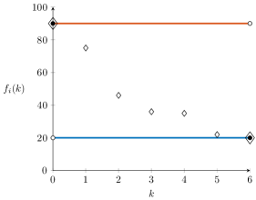
(a) Two data points.

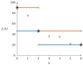
(b) Three data points.

Figure 1: Non-convex cost functions. Evaluated and non-evaluated points are indicated by large and small diamonds, respectively. If $f_{i}(k)$ is evaluated for only a few values of $k$, we have an upper (red) and lower (blue) bound for the non-evaluated points. Discontinuity points are indicated by circles.

We proceed by constructing lower and upper bounds. Define the evaluation indicator

$$v_{i,k}=\begin{cases}1&\text{ if }f_{i}(k)\text{ has been evaluated}\\ 0&\text{otherwise,}\end{cases}$$ (2)

and let $V$ denote the matrix with elements $v_{i,k}$. For a given evaluation matrix $V$ one can construct lower and upper bound cost functions $l_{i},u_{i}:\{0,\dotsc,b_{i}\}\mapsto\mathbb{R}$ for each player $i$. The lower and upper bounds on $f_{i}(k)$ are given by

$$l_{i}(k) =\max\{0,\max_{p\geq k}f_{i}(p)v_{i,p}\}$$ (3a)

$$u_{i}(k) =\min\{M,\min_{q\leq k}f_{i}(q)v_{i,q}\}.$$ (3b)

If $v_{i,p}=1$ for some $p\geq k$ then the lower bound is always attained at the smallest such $p$ because $f_{i}(p)$ is decreasing in $p$. For the same reason, if $v_{i,q}=1$ for some $q\leq k$ then the upper bound is always attained at the largest such $q$. For evaluated points $f_{i}(k)$, the lower and upper bounds coincide. Let $l(\bm{x}):=\sum_{i}l_{i}(x_{i})$ and $u(\bm{x}):=\sum_{i}u_{i}(x_{i})$. Then it holds that $z^{\ast}(l)\leq z^{\ast}(f)\leq z^{\ast}(u)$.

2.2 Bounds for convex cost functions

If cost functions are known to be convex, better lower and upper bounds can be obtained. Figure 2 gives an example for a single convex (non-increasing) cost function $f_{i}:\{0,\dotsc,b_{i}\}\rightarrow[0,M]$, with $b_{i}=6$. In Figure 2(a) two points are evaluated: $f_{i}(0)$ and $f_{i}(6)$. The horizontal blue line illustrates that the value $f_{i}(6)$ is a lower bound for $f_{i}(k)$ for all $k$, because $f_{i}$ is non-increasing. Furthermore, due to convexity of $f_{i}$ the red line connecting the two points is an upper bound for all $f_{i}(k)$, $k=0,\dotsc,b_{i}$. In Figure 2(b) the point $f_{i}(3)$ is also evaluated. The lines through $f_{i}(0)$ and $f_{i}(3)$, and $f_{i}(3)$ and $f_{i}(6)$ yield new upper bounds (red) and/or lower bounds (blue) for non-evaluated points $f_{i}(k)$, $k\in\{0,\dotsc,b_{i}\}$. The best lower and upper bounds are indicated with solid lines.

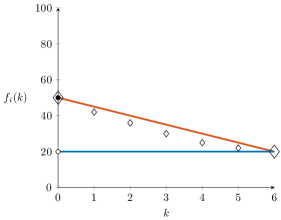
(a) Two data points

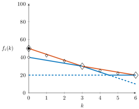
(b) Three data points.

Figure 2: Convex cost functions. Evaluated and non-evaluated points are indicated by large and small diamonds, respectively. If $f_{i}(k)$ is evaluated for only a few values of $k$, we have an upper (red) and lower (blue) bound for the non-evaluated points. The best bounds are indicated by solid lines, redundant bounds are not displayed. Discontinuity points are indicated by circles.

We will construct the upper bound value $u_{i}(k)$ for a particular unobserved point $f_{i}(k)$; the lower bound is analogous. First, we note that if $v_{i,p}=0$ for all $p=0,\dotsc,b_{i}$ for the given $i$, then $f_{i}(k)\leq M$ is an upper bound. Second, if $q>k$ and $v_{i,q}=1$ then

$$f_{i}(k)\leq M\frac{q-k}{q}+f_{i}(q)\frac{k}{q},$$ (4)

because $f_{i}(p)\leq M$. Third, if $p<k$ and $v_{i,p}=1$ then

$$f_{i}(k)\leq f_{i}(p),$$ (5)

because $f_{i}$ is non-increasing. Lastly, if $p<k<q$ and $v_{i,p}=v_{i,q}=1$ then the line connecting these two data points constitutes an upper bound:

$$f_{i}(k)\leq f_{i}(p)\frac{q-k}{q-p}+f_{i}(q)\frac{k-p}{q-p},$$ (6)

because $f_{i}(k)$ is convex. Note that if $p<q<k$ or $k<p<q$ then this line provides a lower bound on $f_{i}(k)$. Lower bounds are obtained similarly. Similar to Section 2.1, let $l_{i},u_{i}:\{0,\dotsc,b_{i}\}\mapsto\mathbb{R}$ denote the functions with the tightest lower and upper bounds for the cost function of player $i$. For evaluated points $f_{i}(k)$, the lower and upper bounds coincide. Again, let $l(\bm{x}):=\sum_{i}l_{i}(x_{i})$ and $u(\bm{x}):=\sum_{i}u_{i}(x_{i})$, and we obtain bounds $z^{\ast}(l)\leq z^{\ast}(f)\leq z^{\ast}(u)$.

2.3 1-Opt method

The 1-Opt method can start at any feasible solution, and aims to improve the objective value in each iteration, by moving a single item from one player to another. One beneficial property is that the initial allocation can be varied based on problem specific information.

The 1-Opt method assumes that for each player $i$ two adjacent points on the cost curve are evaluated, and that the set of evaluated points admits an initial allocation $\bm{x}^{0}$. In each iteration, the method starts with the optimal allocation restricted to only the evaluated data points, and evaluates a single additional point that is adjacent to those already evaluated. The selected new point is the one for which evaluation yields the highest best-case improvement. If the evaluation of such an adjacent point cannot lead to a direct improvement over the current allocation, the method terminates.

Let $\bm{x}^{t}$ denote the allocation at the start of iteration $t$. For each player $i$, let $\theta_{i}$ and $\eta_{i}$ denote the lower bound on the marginal degradation and the upper bound on the marginal gain, respectively:

$$l_{i}(x_{i}^{t}-1)-f_{i}(x_{i}^{t})$$ (7a)

$$\eta_{i}^{t} =f_{i}(x_{i}^{t})-l_{i}(x_{i}^{t}+1).$$ (7b)

In each iteration, $S^{-}$ is the set of players from who an item can be removed, and $\min_{i\in S^{-}}\{\theta_{i}^{t}\}$ is the minimum (i.e., best case) cost increase from removing an item from an eligible player. Similarly, $S^{+}$ is the set of players to who an extra item can be allocated, and $\max_{j\in S^{+}}\{\eta_{j}^{t}\}$ is the maximum (i.e., best case) cost decrease from adding an item to an eligible player. Let $d^{t}$ denote the difference:

$$d^{t}:=\max_{\begin{subarray}{c}i\in S^{-},j\in S^{+}\\ i\neq j\end{subarray}}\{\eta_{j}^{t}-\theta_{i}^{t}\}.$$ (8)

As long as $d$ is strictly larger than zero it may be possible to improve the current allocation by moving a single item (i.e., a 1-opt step).

In each iteration $t$, the method considers all players $i\in S^{+}$ with $v_{i,x_{i}^{t}+1}^{t}=0$, i.e., the players for whom the direct cost decrease after addition of an item is unknown. For such a player $i$, evaluating point $f_{i}(x_{i}^{t}+1)$ yields a best-case improvement of

$$\Delta_{i}^{+,t}=\eta_{i}^{t}-\min_{j}\{\theta_{j}^{t}:j\in S^{-}\backslash\{i\},\leavevmode\nobreak\ v_{j,x_{j}^{t}-1}=1\}.$$ (9)

For other players $i$ set $\Delta_{i}^{+,t}=-\infty$. Allocating an additional item to player $i$ will in the best-case scenario yield an improvement $\eta_{i}$ for that player. The inner minimization in (9) removes the item from the player with the lowest (known) deterioration. Similarly, the method considers all players $i\in S^{-}$ with $v_{i,x_{i}^{t}-1}^{t}=0$, i.e., the players for who the direct cost increase after removal of an item is unknown. For such a player $i$, evaluating point $f_{i}(x_{i}^{t}-1)$ yields a best-case improvement of

$$\Delta_{i}^{-,t}=\max_{j}\{\eta_{j}^{t}:j\in S^{+}\backslash\{i\},\leavevmode\nobreak\ v_{j,x_{j}^{t}+1}=1\}-\theta_{i}^{t},$$ (10)

For other players $i$ set $\Delta_{i}^{-,t}=-\infty$.

Let $i_{t}$ be the maximizer of $\max_{i}\max\{\Delta_{i}^{-,t},\Delta_{i}^{+,t}\}$. Then, either point $f_{i_{t}}(x_{i_{t}}^{t}-1)$ or point $f_{i_{t}}(x_{i_{t}}^{t}+1)$ is evaluated in the current iteration. Subsequently, the optimal allocation on the current set of evaluated points is determined, and the next iteration starts.

For convex cost functions, the current allocation is changed as follows. If the true cost change (as opposed to the best-case change) is indeed negative, the current allocation is changed according to the 1-opt step. One item is added (if $\Delta_{i_{t}}^{+,t}>\Delta_{i_{t}}^{-,t}$) or removed (if $\Delta_{i_{t}}^{+,t}<\Delta_{i_{t}}^{-,t}$) from player $i_{t}$. This item is taken from or moved to player $j_{k}$, the optimizer7 of the inner minimization/maximization of (9) or (10). In case of convex cost functions, this 1-opt step is the only change to the allocation in each iteration. On the other hand, for non-convex cost functions it is possible that after a function evaluation there are multiple changes to the current allocation. To ensure the optimal allocation over all currently evaluated points, resource allocation problem (1) is solved with the additional constraint that only evaluated data points can be used. Pseudocode is given by Algorithm 1.

begin

       Set $t=0$, set $V^{0}$ according to initial information, and determine $l^{0}$;

       Solve $P(f)$ restricted to evaluated data points;

       Denote the solution by $\bm{x}^{0}$;

       Let $S^{-}=\{i:x_{i}^{0}>0\}$ and determine $\theta_{i}^{0}$ for all $i\in S^{-}$;

       Let $S^{+}=\{j:x_{j}^{0}<b_{j}\}$ and determine $\eta_{j}^{0}$ for all $j\in S^{+}$;

       Set $d^{0}=\max\{\eta_{j}^{0}-\theta_{i}^{0}\leavevmode\nobreak\ |\leavevmode\nobreak\ i\in S^{-},j\in S^{+},i\neq j\}$;

       while $d^{t}>0$ do

             for $i=1:n$ do

                   if $i\in S^{+}\land v_{i,x_{i}^{t}+1}^{t}=0$ then

                         $\Delta_{i}^{+,t}=\eta_{i}^{t}-\min_{j}\{\theta_{j}^{t}:j\in S^{-}\backslash\{i\},\leavevmode\nobreak\ v_{j,x_{j}^{t}-1}^{t}=1\}$;

                   else

                        $\Delta_{i}^{+,t}=-\infty$;

                   end if

                  if $i\in S^{-}\land v_{i,x_{i}^{t}-1}^{t}=0$ then

                         $\Delta_{i}^{-,t}=\max_{j}\{\eta_{j}^{t}:j\in S^{+}\backslash\{i\},\leavevmode\nobreak\ v_{j,x_{j}^{t}+1}^{t}=1\}-\theta_{i}^{t}$;

                   else

                        $\Delta_{i}^{-,t}=-\infty$;

                   end if

                  

             end for

            Set $i_{t}\in\operatorname*{arg\,max}_{i}\max\{\Delta_{i}^{-,t},\Delta_{i}^{+,t}\}$;

             if $\Delta_{i_{t}}^{-,t}<\Delta_{i_{t}}^{+,t}$ then

                   Set $\lambda_{t}=1$ and let $j_{t}\in\operatorname*{arg\,min}_{j}\{\theta_{j}^{t}:j\in S^{-}\backslash\{i_{t}\},\leavevmode\nobreak\ v_{j,x_{j}^{t}-1}^{t}=1\}$;

                  

            else

                   Set $\lambda_{t}=-1$ and let $j_{t}\in\operatorname*{arg\,max}_{j}\{\eta_{j}^{t}:j\in S^{+}\backslash\{i_{t}\},\leavevmode\nobreak\ v_{j,x_{j}^{t}+1}^{t}=1\}$;

                  

             end if

            Set $V^{t+1}=V^{t}$;

             Evaluate $f_{i_{t}}(x_{i_{t}}^{t}+\lambda_{t})$ and set $v_{i,x_{i_{t}}^{t}+\lambda_{t}}^{t+1}=1$;

             Solve $P(f)$ restricted to evaluated data points;

             Denote the solution by $\bm{x}^{t+1}$;

             Determine $l^{t+1}$;

             Let $S^{-}=\{i:x_{i}^{t+1}>0\}$ and determine $\theta_{i}$ for all $i\in S^{-}$;

             Let $S^{+}=\{j:x_{j}^{t+1}<b_{j}\}$ and determine $\eta_{j}$ for all $j\in S^{+}$;

             Set $d^{t}=\max\{\eta_{j}^{t}-\theta_{i}^{t}\leavevmode\nobreak\ |\leavevmode\nobreak\ i\in S^{-},j\in S^{+},i\neq j\}$;

             Set $t\leftarrow t+1$;

            

       end while

      Set $\bm{x}^{\text{1-opt}}=\bm{x}^{t}$;

      

end

Algorithm 1 1-Opt method

The following lemma shows that the 1-Opt method guarantees the optimal solution for convex cost functions.

Lemma 1.

Let cost functions $f_{i}:\{0,\dotsc,b_{i}\}\rightarrow[0,M]$ be convex and non-increasing for all $i=1,\dotsc,n$. Then the 1-Opt solution $\bm{x}^{\text{1-opt}}$ is optimal to (1).

Proof.

The 1-Opt method terminates with solution $\bm{x}^{\text{1-opt}}$ if and only if $d\leq 0$. This is equivalent to

$$\max_{\begin{subarray}{c}i\in S^{-},j\in S^{+}\\ i\neq j\end{subarray}}\Big{\{}\big{(}f_{j}(x_{j}^{\text{1-opt}})-l_{j}(x_{j}^{\text{1-opt}}+1)\big{)}-\big{(}l_{i}(x_{i}^{\text{1-opt}}-1)-f_{i}(x_{i}^{\text{1-opt}})\big{)}\Big{\}}\leq 0.$$ (11)

Thus, for each pair $(i,j)\in S^{-}\times S^{+}$ with $i\neq j$ the following inequalities hold:

$$\begin{aligned} f_{j}(x_{j}^{\text{1-opt}})-f_{j}(x_{j}^{\text{1-opt}}+1)\leq&f_{j}(x_{j}^{\text{1-opt}})-l_{j}(x_{j}^{\text{1-opt}}+1)\\ \leq&l_{i}(x_{i}^{\text{1-opt}}-1)-f_{i}(x_{i}^{\text{1-opt}})\\ \leq&f_{i}(x_{i}^{\text{1-opt}}-1)-f_{i}(x_{i}^{\text{1-opt}}),\end{aligned}$$ (12)

where the first and last inequalities holds because $l_{i}(k)$ is a lower bound to $f_{i}(k)$ for all $i,k$. The first term is the ‘true’ cost decrease of assigning an extra item to an eligible player $i$, and the last term is the true cost increase of removing an item from another eligible player $j$. The decrease is smaller than the increase for any player pair $(i,j)$, so moving any item from one player to another cannot yield an improvement to the current allocation.

Due to convexity of cost functions $f_{i}$, moving multiple items cannot yield an improvement either. With each additional item involved, the minimum cost increase of removing the item from one player will grow, while the maximum cost decrease of adding the item to another player will diminish. Thus, the current allocation $\bm{x}^{\text{1-opt}}$ is optimal to (1). ∎

The number of function evaluations depends largely on the set of initially evaluated points. Without problem specific information, one can start with a uniform initialization of matrix $V$, e.g., one can evaluate the points associated with $\lfloor B/n\rfloor$ and $\lfloor B/n\rfloor+1$ items for each player (if this is feasible).

The 1-Opt method maintains feasibility in each iteration, and the objective value of the current allocation is always exactly known. Thus, if the method is terminated in any iteration $t$, the current solution $\bm{x}^{t}$ can directly be implemented. Its objective value is an upper bound for the objective value of the final allocation $\bm{x}^{\text{1-opt}}$.

2.4 Sandwich method

The 1-Opt method is a heuristic if the cost functions are not known to be convex. In this section we present a method that yields the optimal solution to the resource allocation problem for both convex and non-convex cost functions. The sandwich method (SW) directly uses the lower and upper bound cost function $l$ and $u$ on the true cost function $f$ that are presented in Section 2.2 and Section 2.1. The sandwich method is inspired by Siem et al., (2011), who use sandwich methods, both with and without derivative information, to approximate univariate convex functions.

Let $l^{t}$ and $u^{t}$ denote the lower and upper bound cost functions at the start of iteration $t$. In every iteration $t$, we solve the lower bound problem, to obtain objective value $z^{\ast}(l^{t})$ and optimal solution $\bm{x}^{l,t}$. The value $z^{\ast}(l^{t})=z(\bm{x}^{l,t},l^{t})$ is a lower bound to the true optimal objective value $z^{\ast}(f)$. Additionally, $z(\bm{x}^{l,t},u^{t})$ is an upper bound. The sandwich method uses these bounds to formulate an objective value gap. Define

$$g^{t}:=z(\bm{x}^{l,t},u^{t})-z(\bm{x}^{l,t},l^{t}).$$ (13)

The SW method iteratively improves the lower and upper bounds on the objective value as more data points have been evaluated, and the goal is to evaluate those points that reduce the gap between the upper and lower bound objective value the most. Thus, it ‘sandwiches’ the true cost function (and objective value). As soon as the gap is small enough the method terminates. Solution $\bm{x}^{l,t}$ is the final solution, and the objective value is in the interval $[z(\bm{x}^{l,t},l^{t}),z(\bm{x}^{l,t},u^{t})]$. Note that in any iteration $t$ the value $z(\bm{x}^{u,t},u^{t})$ is also an upper bound on the final objective value, but it is not an upper bound for the objective value corresponding to allocation $\bm{x}^{l,t}$.

As long as the gap $g^{t}$ is larger than a pre-specified tolerance $\epsilon$, a new iteration starts in which a new point $f_{i}(k)$ is evaluated; this point is chosen according to some decision rule DR. With $\epsilon=0$ the sandwich method guarantees optimality, both for convex and non-convex cost functions. Pseudocode is given by Algorithm 2.

begin

       Set $t=0$, Pick $\epsilon>0$, set $V^{0}$ according to initial information;

       Determine $l^{0},u^{0}$, solve $P(l^{0})$ and determine $g^{0}$;

       while $g^{t}>\epsilon$ do

             Let $(i,k)=\text{DR}(V^{t},l^{t},u^{t})$;

             Evaluate $f_{i}(k)$ and determine $V^{t+1}$;

             Determine cost functions $l^{t+1}$ and $u^{t+1}$;

             Solve $P(l^{t+1})$ and let $\bm{x}^{l,t+1}$ denote the solution;

             Determine $g^{t+1}$;

             Set $t\leftarrow t+1$;

            

       end while

      Set $\bm{x}^{\text{sw}}=\bm{x}^{l,t}$;

      

end

Algorithm 2 Sandwich method

The corresponding objective value is $z(\bm{x}^{\text{sw}},f)$. Irrespective of the chosen decision rule, this is within $\epsilon$ of the global optimum.

Lemma 2.

Let cost functions $f_{i}:\{0,\dotsc,b_{i}\}\mapsto[0,M]$ be convex and non-increasing for all $i=1,\dotsc,n$. Then it holds that $z(\bm{x}^{\text{sw}},f)\leq z^{\ast}(f)+\epsilon$.

Proof.

Let $l^{t}$ and $u^{t}$ denote the lower and upper bound matrices at the start of iteration $t$. Let $\bm{x}^{\ast}$, $\bm{x}^{l,t}$ and $\bm{x}^{u,t}$ be minimizers of $P(f)$, $P(l^{t})$ and $P(u^{t})$, respectively. Then the following sequence of lower bounds holds for $z^{\ast}(f)$:

$$z^{\ast}(l^{t})=z(\bm{x}^{l,t},l^{t})\leq z(\bm{x}^{\ast},l^{t})\leq z(\bm{x}^{\ast},f)=z^{\ast}(f).$$ (14)

The first inequality holds because $\bm{x}^{\ast}$ is feasible for $P(l^{t})$ but not necessarily optimal. The second inequality holds because $l_{i}(k)\leq f_{i}(k)$ for all $i,k$. Similarly, the following sequence of upper bounds holds:

$$z(\bm{x}^{l,t},u^{t})\geq z(\bm{x}^{u,t},u^{t})=z^{\ast}(u^{t})\geq z(\bm{x}^{u,t},f)\geq z(\bm{x}^{\ast},f)=z^{\ast}(f).$$ (15)

The first inequality holds because $\bm{x}^{l,t}$ is feasible for $P(u^{t})$ but not necessarily optimal. The second inequality holds because $u_{i}(k)\geq f_{i}(k)$ for all $i,k$, and the third inequality holds because $\bm{x}^{u,t}$ is feasible for $P(f)$ but not necessarily optimal. Thus, at any iteration $t$ the following holds for solution $\bm{x}^{L,t}$:

$$z(\bm{x}^{L,t},l^{t})\leq z^{\ast}(f)\leq z(\bm{x}^{L,t},u^{t}).$$ (16)

By construction, if at iteration $t$ the condition

$$z(x_{i}^{L,t},f)\leq z^{\ast}(f)+\epsilon,$$ (17)

does not hold, a new function value $f_{i}(k)$ is evaluated for some $i,k$ in the next iteration in order to reduce the gap. After $n+\bm{b}^{\top}\bm{e}$ iterations, all values $f_{i}(k)$ have been evaluated for all $k\in\{0,\dotsc,b_{i}\}$ and all $i=1,\dotsc,n$, so $l_{i}(k)=f_{i}(k)=u_{i}(k)$ for all $i,k$, and the inequalities in (16) reduce to equalities. Thus, after at most $n+\bm{b}^{\top}\bm{e}$ iterations the condition (17) must be satisfied. ∎

It remains to specify the decision rule DR that picks the new data point to be evaluated in each iteration. Several options are presented below:

• Random (SW-RND): Randomly picks a point $(i,k)$ that has not been evaluated yet at the start of iteration $t$, i.e., with $v_{i,k}^{t}=0$.

• Maximum difference - all points (SW-A): Determines for all $(i,k)$ the difference between upper bound $u_{i}^{t}(k)$ and lower bound $l_{i}^{t}(k)$ for the given set of evaluated data points $V^{t}$ at the start of iteration $t$. It then evaluates the data point for which this difference is largest.

• Maximum difference - restricted to points in $\bm{x}^{l,t}$ and/or $\bm{x}^{u,t}$ (SW-R): Similar to decision rule SW-A, except that in each iteration only those data points are considered that were chosen in the current allocation $\bm{x}^{l,t}$ and/or $\bm{x}^{u,t}$. If no such points exist, it falls back on SW-A. Note that this rule additionally solves ILP $P(u^{t})$ in each iteration.

Decision rule SW-R is expected to perform best; SW-RND and SW-A are included in the numerical experiments to illustrate the influence of the employed decision rule.

As a fourth decision rule, we also considered amending SW-R to consider only those data points that were chosen either in the allocation $\bm{x}^{l,t}$ or $\bm{x}^{u,t}$, but not both. The rationale is that for such points, the true value may provide more information than for points that are chosen in both allocations. For the latter, the point is chosen regardless of whether its value is at the lower or upper bound, so allocations are not sensitive to its value. Preliminary experiments indicate that in many iterations $t$ there are no not yet evaluated points that are chosen in $\bm{x}^{l,t}$ or $x^{u,t}$, but not both. Thus, this decision rule often falls back on SW-R, and is not considered further in the numerical experiments in Section 3.

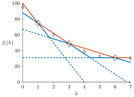
(a) Player 1. The points $f_{1}(1)$, $f_{1}(3)$ and $f_{1}(6)$ have been evaluated.

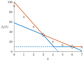
(b) Player 2. The points $f_{2}(3)$ and $f_{2}(6)$ have been evaluated.

Figure 3: Illustration of sandwich method using convexity-based bounds, with allocation budget $B=9$ and upper bound $M=100$. Evaluated and non-evaluated points are indicated by large and small diamonds, respectively. Lower bounds are blue and upper bound are red; the best bounds are indicated by solid lines, redundant bounds are not displayed. The lower bound solution is $\bm{x}^{l}=(5,4)$ and the upper bound solution is $\bm{x}^{u}=(4,5)$.

Figure 3 illustrates the SW method for a situation with two players; for player 1 three points are evaluated and for player 2 two points are evaluated. There are in total 11 non-evaluated points. If decision rule SW-RND is used to determine the next evaluated point, one of these points is selected at random. Decision rule SW-A evaluates point $f_{2}(0)$, for it has the largest gap. For decision rules SW-R, the solutions to $P(l)$ and $P(u)$ are taken into account. The lower bound solution in the current evaluation is $\bm{x}^{l}=(5,4)$ and the upper bound solution is $\bm{x}^{u}=(4,5)$. Among these four points, the gap at $f_{2}(4)$ is largest: this point is evaluated by SW-R.

2.5 Illustration of evaluated points

To compare and contrast the solution methods, Figure 4 illustrates the progress of the methods 1-Opt, SW-RND, SW-A and SW-R for two instances with convex and non-convex cost functions ($n=3$, $b_{i}=7$ for all $i$, $B=10$).

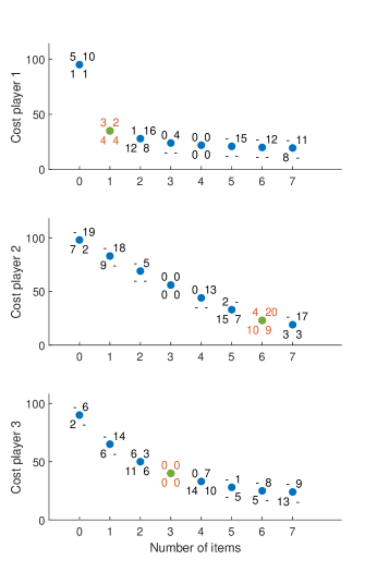
(a) Convex cost functions.

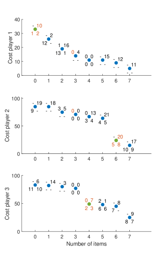
(b) Non-convex cost functions.

Figure 4: Illustration of solution method progress on instances with 3 players, for convex and non-convex cost functions. Per (player, data point), the two numbers indicate in what iteration that point was evaluated for the methods 1-Opt (top left), SW-RND (top right), SW-A (bottom left) and SW-R (bottom right). If the data point is the final allocation for that player for a method, the number is colored red. The symbol ‘-’ indicates that the point was not evaluated by the method. The optimal allocation is indicated with green dots. Vertical axis shifted left for presentation clarity.

In Figure 4(a) (convex), the cost function for player 1 has a fast initial drop and marginal improvements after that. For player 2 the improvement rate is near constant, and for player 3 a gradually diminishing improvement can be observed. Overall, 1-Opt, SW-RND, SW-A and SW-R require $12$, $23$, $18$ and $13$ function evaluations, respectively. All methods find the optimal allocation with objective value $98.0$. Method 1-Opt starts with evaluating $f_{i}(3)$ and $f_{i}(4)$ for all players. For player 1, it subsequently evaluates data points to the left, whereas for player 2 it evaluates data points to the right of the initial points. For player 3 it evaluates only a single additional point. All sandwich methods start with the initial evaluation of $f_{1}(4)$, $f_{2}(3)$ and $f_{3}(3)$. SW-RND randomly chooses the next points to evaluate, which results in evaluating nearly all points. SW-A and SW-R perform significantly better. SW-A evaluates roughly the same points as 1-Opt. However, it can evaluate non-adjacent points, e.g., for player 2 it evaluates $f_{2}(k)$ for $k=0,3,5,6,7$.

In Figure 4(b) (non-convex), the cost function for player 1 is non-convex, but decreases gradually (note the difference in vertical axis scaling). The cost functions for players 2 and 3 exhibit drops of larger magnitudes that lead to non-convexity. Method 1-Opt results in an allocation with objective value 134 (9 function evaluations). The sandwich methods all yield the optimal objective value of 106; SW-RND requires 24 function evaluations (i.e., it evaluates all points), SW-A 16 function evaluations and SW-R 13 function evaluations. After a few iterations, 1-Opt cannot find any point where evaluating may result in a direct improvement, and thus terminates. Consequently, it finds only a locally optimal solution.

2.6 Extensions

The problem formulation (1) can be adapted in various ways. A more general version is obtained by replacing budget constraint (1b) by a general linear or convex constraint. Both the 1-Opt and the sandwich method can be applied to such formulations as well, but for ease of exposition we used a simple linear constraint. Another more general version of (1) is obtained by letting $\varphi:\mathbb{R}^{n}\mapsto\mathbb{R}$ and using the composite objective

$$\varphi(f_{1}(x_{1}),\dotsc,f_{n}(x_{n})),$$ (18)

where $\varphi(\cdot)$ is an explicitly known function, e.g., the pointwise maximum function. The inequalities (14) and (15) in the proof of Lemma 2 remain valid, so the sandwich method can be applied to this more general version. The local search concept of the 1-Opt method can be extended to more general composite objective functions as well. However, this requires several modifications, as its current formulation utilizes operations that are specific to the sum function.

3 Numerical experiments

We test the solution methods on both randomly generated test instances and instances stemming from applications. Section 3.1 describes the setup of the numerical experiments: the used benchmark methods and initialization. In Section 3.2 and Section 3.3, we report and discuss the performance of the solution methods on randomly generated instances with convex and non-convex cost functions, respectively. Section 3.4 considers solution guarantees when the methods are terminated early. In Section 3.5, the methods are applied to instances from two applications in radiation therapy treatment planning. In the numerical experiments, problems of form (1) are solved via their ILP representation (see Appendix A) using Gurobi 9.0 (Gurobi Optimization LLC, , 2022).

3.1 Setup

To put the performance of the 1-Opt method and the sandwich methods into perspective, we compare the methods with three benchmark methods in terms of their obtained objective value and number of function evaluations. The first benchmark method is the NOMAD solver (Audet et al., , 2022), which is the best performing open-source derivative-free solver in our preliminary numerical experiments (see Section 1.5). NOMAD does not guarantee an optimal solution, neither for the convex nor the non-convex instances. By default, NOMAD does not consider separability of cost functions but only tracks evaluations of the entire cost function $f(\bm{x})$. As such, it does not track function evaluations of cost functions $f_{i}$ for individual players $i$. In the numerical experiments, this is registered using a custom callback function. However, this does mean that NOMAD may perform iterations without considering new values of $f_{i}(x_{i})$ for any player $i$. Consequently, it does not necessarily recognize that all individual cost functions have been fully evaluated and thus may not terminate at that time.

The other two benchmark methods are simple constructive methods: the myopic method (MY) and the prescient method (PR). The myopic method is a greedy method that starts with zero items allocated, and allocates in each iteration a single item to the player with the largest immediate gain. Section C.1 describes the myopic method. The prescient method is similar to the myopic method, but is less greedy. It takes into account the average gain over the remaining horizon for each player, and also assigns items to a player if its immediate gain is low, but its average gain is high. Section C.2 describes the prescient method. Both the myopic and the prescient method guarantee the optimal allocation for convex cost functions, but are heuristics for non-convex cost functions.

For the initialization of the 1-Opt method, for each player both the data points corresponding to $\lfloor B/n\rfloor$ and $\lfloor B/n\rfloor+1$ items are evaluated to obtain $V^{0}$. For the sandwich methods we set $\epsilon=0$, to ensure optimality of the allocations. Matrix $V^{0}$ is set as follows. We assign $\lfloor B/n\rfloor$ to each player. The remaining allocation budget $B-n\lfloor B/n\rfloor$ is evenly allocated, starting from player one; let $\bm{x}^{0}$ denote the resulting allocation. Matrix $V^{0}$ is obtained by evaluating all data points corresponding to $\bm{x}^{0}$.

3.2 Randomly generated convex cost functions

3.3 Randomly generated non-convex cost functions

3.4 Early termination

3.5 Two applications in radiation therapy planning

Radiation therapy (RT) is one of the predominant treatment modalities for cancer, and treatment planning for RT relies heavily on mathematical optimization. In the current section, we describe two applications in RT treatment planning that give rise to resource allocation problems with expensive function evaluations, and illustrate the developed methods on instances of both applications.

In both applications, the allocation cost functions need not be convex in theory, but they are near-convex in practice. This means that 1-Opt and the benchmark methods MY, PR do not guarantee optimality. For 1-Opt and the sandwich methods, we report results using bounds with and without the convexity assumption. Note that if the convexity assumption is used while cost functions are in fact not convex, the sandwich methods lose their optimality guarantee. However, with the convexity assumption tighter lower and upper bounds are obtained, which might translate to fewer function evaluations.

Proton therapy slot allocation

Volumetric modulated arc therapy

4 Conclusion

In practical applications of resource allocation problems, evaluating the objective function for a given number of resources can be expensive. Thus, it may be necessary to use only few function evaluations during the decision-making process. However, current solution methods for resource allocation problems do not take this aspect into account. At the same time, derivative-free integer optimization methods do not properly use the separable objective structure that is typically encountered in resource allocation problems. To bridge this gap, we introduced solution methods for integer resource allocation problems that aim to limit the number of function evaluations. We have considered formulations with both convex and non-convex separable cost functions; for convex cost functions both the 1-Opt and sandwich methods guarantee an optimal solution. For non-convex cost functions, only the sandwich methods guarantee optimality.

From our numerical experiments, we conclude that for convex cost functions the sandwich method SW-R requires fewest function evaluations on large-scale instances, and 1-Opt is comparable to SW-R for small instances. For non-convex cost functions, 1-Opt uses fewer function evaluations than SW-R, but is prone to getting stuck in a local minimum. This may result in substantially worse allocations than the sandwich methods (which are exact by construction). Depending on the instance type, the presented methods have a function evaluation percentage between $21\%$ and $63\%$ (of the maximum number of function evaluations), and consistently outperform several benchmark methods including the NOMAD solver.

In practical applications, cost functions may be ‘near-convex’, as demonstrated in two application stemming from radiation therapy. In those cases, 1-Opt can provide a near-optimal solution while substantially outperforming the sandwich methods in number of function evaluations. The numerical results indicate that both the choice of bounds (with or without convexity assumption) and the starting point can influence the resulting objective value and the required number of function evaluations. For implementation of the presented solution methods in particular applications, both of these topics require further research.

Appendix A ILP representation

Resource allocation problem (1) is equivalent to the following integer (binary) linear programming (ILP) problem:

$$P(F)\leavevmode\nobreak\ =\leavevmode\nobreak\ \leavevmode\nobreak\ \leavevmode\nobreak\ \min_{\bm{y}}\leavevmode\nobreak\ \leavevmode\nobreak\ \sum_{i=1}^{n}\sum_{k=0}^{b_{i}}F_{i,k}y_{i,k}$$ (A.1a)

s.t. $$\leavevmode\nobreak\ \sum_{i=1}^{n}\sum_{k=0}^{b_{i}}ky_{i,k}=B$$ (A.1b)

$$\leavevmode\nobreak\ y_{i,k}\in\{0,1\},\leavevmode\nobreak\ \forall k=0,\dotsc,b_{i},\forall i=1,\dotsc,n,$$ (A.1c)

with $F_{i,k}=f_{i}(k)$, for all $k=1,\dotsc,b_{i}$, and $i=1,\dotsc,n$. For known objective coefficients, problem (A.1) can be solving using any standard ILP solver. The optimal allocation $\bm{x}^{\ast}$ can be recovered from an optimal solution $\bm{y}^{\ast}$ via $\bm{x}_{i}=\sum_{k=0}^{b_{i}}ky_{i,k}$ for all $i$.

Appendix B Radiation therapy data

Figure 1(a) plots the BED for all patients $i=1,\dotsc,17$ as a function of the number of allocated proton slots, for the proton therapy example in Section 3.5. Figure 1(b) plots the fluence map matching inaccuracy $h_{m}$ for all arc segments $m=1,\dotsc,36$ as a function of time (sec), for the VMAT example in Section 3.5.

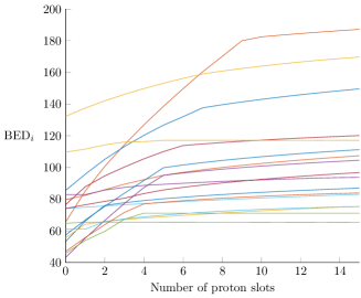
(a) Payoff functions $\text{BED}_{i}$ for patient
$i=1,\dotsc,17$.

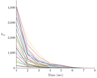
(b) Fluence map matching inaccuracy functions $h_{m}$ for arc segments $m=1,\dotsc,36$.

Figure B.1: Cost functions for the radiation therapy examples in Section 3.5.

Appendix C Benchmark methods

C.1 Myopic method

The myopic method (MY), or greedy method, is an iterative procedure where in each iteration a single item is allocated to a player with the largest immediate gain. For an allocation $\bm{x}^{t}$ at the start of iteration $t$, the immediate gain of getting an extra item for player $i$ is given by

$$G_{i}(x_{i}^{t})=f_{i}(x_{i}^{t})-f_{i}(x_{i}^{t}+1),$$ (C.1)

which is non-negative, because $f_{i}$ is non-increasing. The method initializes by computing the immediate gain at zero items for each player $i$, i.e., evaluating $f_{i}(0)$ and $f_{i}(1)$. Then, the player $i$ with the highest immediate gain is assigned the item and its new immediate gain is computed, unless the player $i$ has reached its individual allocation budget $b$. The myopic method starts with $2n$ function evaluations. After that, it performs $B$ allocation iterations. Except for the last iteration, each of these requires at most one additional function evaluation. Thus, the total number of black-box function evaluations for the myopic method is at most $2n+B-1$.

The total allocation budget $B$ has a large influence on the performance. For instances with a high total allocation budget, we can start with $x_{i}^{0}=b_{i}$ for all players $i$ (i.e., assigning $\bm{b}^{\top}\bm{e}$ items), and remove items until feasible. In particular, in each iteration we remove the item for the player $i$ whose gain for their currently last item is smallest. It is easy to show that if $2B>\bm{b}^{\top}\bm{e}$ this requires less iterations in the worst-case than starting with $x_{i}^{0}=0$ for all $i$. Pseudocode for the case $2B\leq\bm{b}^{\top}\bm{e}$ is given in Algorithm 3. The case with $2B>\bm{b}^{\top}\bm{e}$ is comparable.

begin

       Set $t=0$, and set $S=\{1,\dotsc,n\}$, $J=S$;

       Set $x_{i}^{0}=0$ for all $i\in S$;

       Evaluate $f_{i}(0)$ and $f_{i}(1)$ for all $i\in S$;

       while $t<B$ do

             Determine $G_{i}(x_{i}^{t})$ for all $i\in J$;

             Let $j_{t}\in\operatorname*{arg\,max}_{i\in J}G_{i}(x_{i}^{t})$;

             Set $x_{j_{t}}^{t+1}=x_{j_{t}}^{t}+1$;

             Set $x_{i}^{t+1}=x_{i}^{t}$ for all $i\in S\backslash\{j_{t}\}$;

             if $x_{j_{t}}^{t}+1<b_{i}\leavevmode\nobreak\ \land\leavevmode\nobreak\ t<B-1$ then

                   Evaluate $f_{j_{t}}(x_{j_{t}}^{t}+2)$;

                  

            else

                   Set $J\leftarrow J\backslash\{j_{t}\}$;

                  

             end if

            Set $t\leftarrow t+1$;

            

       end while

      Set $\bm{x}^{\text{ma}}=\bm{x}^{t}$.

end

Algorithm 3 Myopic method for $2B\leq\bm{b}^{\top}\bm{e}$

For convex cost functions the myopic method is exact, as proved in Lemma 3.

Lemma 3.

Let cost functions $f_{i}:\{0,\dotsc,b_{i}\}\rightarrow[0,M]$ be convex and non-increasing for all $i=1,\dotsc,n$. Then the myopic solution $\bm{x}^{\text{ma}}$ is optimal to (1).

Proof.

The proof is given for the case $2B\leq\bm{b}^{\top}\bm{e}$, the case $2B>\bm{b}^{\top}\bm{e}$ is similar. Let $G^{t}$ denote the objective value improvement in iteration $t$ and let $J_{t}=\{i:x_{i}^{t}<b_{i}\}$, i.e., the set of players eligible for allocation in iteration $t$. For all $t\geq 0$ it holds that

$$G^{t} :=\max_{i\in J_{t}}G_{i}(x_{i}^{t})\geq\max_{i\in J_{t+1}}G_{i}(x_{i}^{t+1})=G^{t+1},$$ (C.2)

where the inequality holds due to convexity of $f_{i}$ for all $i$ and the fact that $J_{t+1}\subseteq J_{t}$. With $\bm{x}^{\text{ma}}$ the allocation resulting from the myopic method and $z(\bm{x}^{\text{ma}},f)$ the corresponding objective value, it holds that

$$z(\bm{x}^{\text{ma}},f)= \sum_{i=1}^{n}f_{i}(x_{i}^{\text{ma}})=\sum_{i=1}^{n}f_{i}(0)-\sum_{t=0}^{B-1}G^{t},$$ (C.3)

i.e., the total cost is the sum of individual player costs at the zero allocation minus the gain in each iteration. From (C.2) and (C.3) it follows that allocating a number of $c$ ($\leq B$) extra items to a subset of players in any way decreases (i.e., improves) the objective value by at most $cG^{B}$. To maintain feasibility, $c$ items must be removed from the other players, which increases (i.e., deteriorates) the objective value by at least $G^{B-1}+\dotsc+G^{B-c}$, which is larger than $cG^{B}$. Thus, the current allocation $\bm{x}^{\text{ma}}$ is optimal. ∎

C.2 Prescient method

For non-convex cost functions, the myopic method may have poor performance. This poor performance exhibits particularly in those cases where the immediate gain for a player $i$ at $x_{i}$ is small, but larger gains are possible for higher values of $x_{i}$. To remedy this, we propose a new heuristic that bases decisions both on the immediate gain and the average gain over the remaining horizon for that player. The prescient method (PR) has the same structure as the myopic method and also allocates items one-by-one. With an allocation $\bm{x}^{t}$ at the start of iteration $t$, the maximum number of items that can be allocated to player $i$ is

$$\beta_{i}^{t}(x_{i}^{t}):=\min\{b_{i},x_{i}^{t}+B-t\}.$$ (C.4)

The average improvement for player $i$ over the interval $[x_{i}^{t},\beta_{i}^{t}(x_{i}^{t})]$ is

$$A_{i}(x_{i}^{t}) =\frac{f_{i}(x_{i}^{t})-u_{i}(\beta_{i}^{t}(x_{i}^{t}))}{\beta_{i}^{t}(x_{i}^{t})-x_{i}^{t}},$$ (C.5a)

where the upper bound value $u_{i}(\beta_{i}^{t}(x_{i}^{t}))$ is used because $f_{i}(\beta_{i}^{t}(x_{i}^{t}))$ need not be evaluated. Thus, the reported average gain is conservative. The score of player $i$ at $x_{i}^{t}$ is defined as

$$s_{i}(x_{i}^{t}):=\max\{G_{i}(x_{i}^{t}),A_{i}(x_{i}^{t})\}.$$ (C.6)

In each iteration, the item is allocated to the player $i$ with the currently highest score8. The prescient method starts with $3n$ function evaluations. After that, it performs $B$ allocation iterations. Except for the last iteration, each of these requires at most one additional function evaluation. Thus, the total number of black-box function evaluations for the prescient method is at most $3n+B-1$.

Similar to the myopic method, for instances with a high total allocation budget we can start with $x_{i}^{0}=b_{i}$ for all players $i$ (i.e., assigning $\bm{b}^{\top}\bm{e}$ items), and remove items until feasible. Similar to the myopic method, removing items requires fewer iterations (in the worst-case) than adding items if $2B\leq\bm{b}^{\top}\bm{e}$. Pseudocode for the case $2B\leq\bm{b}^{\top}\bm{e}$ is given in Algorithm 4.

begin

       Set $t=0$, and set $S=\{1,\dotsc,n\}$, $J=S$;

       Set $x_{i}^{0}=0$ for all $i\in S$;

       Evaluate $f_{i}(0)$, $f_{i}(1)$ and $f_{i}(b)$ for all $i\in S$;

       while $t<B$ do

             Determine $s_{i}(x_{i}^{t})$ for all $i\in J$;

             Let $j_{t}\in\operatorname*{arg\,max}_{i\in J}s_{i}(x_{i}^{t})$;

             Set $x_{j_{t}}^{t+1}=x_{j_{t}}^{t}+1$;

             Set $x_{i}^{t+1}=x_{i}^{t}$ for all $i\in S\backslash\{j_{t}\}$;

             if $x_{j_{t}}^{t}+1<b\leavevmode\nobreak\ \land\leavevmode\nobreak\ t<B-1$ then

                   Evaluate $f_{j_{t}}(x_{j_{t}}^{t}+2)$;

                  

             else if $x_{j_{t}}^{t}+1=b$ then

                   Set $J\leftarrow J\backslash\{j_{t}\}$;

                  

             Set $t\leftarrow t+1$;

            

       end while

      Set $\bm{x}^{\text{pa}}=\bm{x}^{t}$;

      

end

Algorithm 4 Prescient method for $2B\leq\bm{b}^{\top}\bm{e}$

For convex cost functions the prescient method is exact, as proved in Lemma 4.

Lemma 4.

Let cost functions $f_{i}:\{0,\dotsc,b_{i}\}\rightarrow[0,M]$ be convex and non-increasing for all $i=1,\dotsc,n$. Then the prescient solution $\bm{x}^{\text{pa}}$ is optimal to (1).

Proof.

Due to convexity of cost functions $f_{i}$, it holds that $G_{i}(x_{i})\geq A_{i}(x_{i})$ and, consequently, $s_{i}(x_{i})=G_{i}(x_{i})$ for all feasible $x_{i}$ and all $i=1,\dotsc,n$. Thus, the prescient method uses the same allocation rule as the myopic method in each iteration, and optimality follows from Lemma 3. ∎

Both presented benchmark methods, the myopic and the prescient method, are optimal for convex cost functions, and the latter requires an equal or higher number of function evaluations than the former. However, for non-convex cost functions the prescient method is expected to perform better because it also accounts for possible non-convexities via the score function (C.6).

In the numerical experiments, we use Algorithms 3 and 4 if $2B\leq\bm{b}^{\top}\bm{e}$. Otherwise, we use their counterparts starting with each player $i$ allocated $b_{i}$ items, and use the described procedure to remove items instead.

Lastly, we note that simple adaptations may improve the myopic and prescient method. For example, the direct gain of a player need not be computed if the (upper bound on the) total possible gain for the player is lower than the direct gain of another player. For ease of exposition, we do not incorporate such adaptations.

References

- Audet and Hare, (2017) Audet, C. and Hare, W. (2017). Derivative-free and blackbox optimization. Springer.
- Audet et al., (2022) Audet, C., Le Digabel, S., Tribes, C., and Rochon Montplaisir, V. (2022). The NOMAD project. https://www.gerad.ca/nomad, Accessed 22-01-2022.
- Balvert and Craft, (2017) Balvert, M. and Craft, D. (2017). Fast approximate delivery of fluence maps for IMRT and VMAT. Phys. Med. Biol., 62(4):1225–1247.
- Brekelmans et al., (2005) Brekelmans, R., Driessen, L., Hamers, H., and den Hertog, D. (2005). Constrained optimization involving expensive function evaluations: a sequential approach. Eur. J. Oper. Res., 160:121–138.
- Bretthauer and Shetty, (2002) Bretthauer, K. M. and Shetty, B. (2002). The nonlinear knapsack problem - algorithms and applications. Eur. J. Oper. Res., 138:459–472.
- Craft et al., (2014) Craft, D., Bangert, M., Long, T., Papp, D., and Unkelbach, J. (2014). Shared data for intensity modulated radiation therapy (IMRT) optimization research: the CORT dataset. GigaScience, 3(1):37.
- Duijzer et al., (2018) Duijzer, L. E., van Jaarsveld, W. L., Wallinga, J., and Dekker, R. (2018). Dose-optimal vaccine allocation over multiple populations. Prod. Oper. Manag., 27(1):143–159.
- Ehrgott et al., (2008) Ehrgott, M., Güler, Ç., Hamacher, H. W., and Shao, L. (2008). Mathematical optimization in intensity modulated radiation therapy. 4OR-Q. J. Oper. Res., 6:199–262.
- Eijgenraam et al., (2014) Eijgenraam, C., Kind, J., Bak, C., Brekelmans, R., den Hertog, D., Duits, M., …, and Kuijken, W. (2014). Economically efficient standards to protect the Netherlands against flooding. Interfaces, 44(1):7–21.
- Fowler, (1989) Fowler, J. F. (1989). The linear-quadratic formula and progress in fractionated radiotherapy. Brit. J. Radiol., 62(740):679–694.
- Gurobi Optimization LLC, (2022) Gurobi Optimization LLC (2022). Gurobi optimizer reference manual. http://www.gurobi.com.
- Hall and Giaccia, (2012) Hall, E. J. and Giaccia, A. J. (2012). Radiobiology for the radiologist. Lippincott Williams & Wilkins. Philadelphia, Pennsylvania, USA.
- Hochbaum, (2007) Hochbaum, D. S. (2007). Complexity and algorithms for nonlinear optimization problems. Ann. Oper. Res., 153:257–296.
- Katoh et al., (2013) Katoh, N., Shioura, A., and Ibaraki, T. (2013). Resource allocation problems. In Pardalos, P. M., Ding-Zhu, D., and Graham, R. L., editors, Handbook of combinatorial optimization, second edition, pages 2897–2988. Springer Reference.
- Kelly et al., (2019) Kelly, M., van Amerongen, J. H. M., Balvert, M., and Craft, D. (2019). Dynamic fluence map sequencing using piecewise linear leaf position functions. Biomed. Phys. Eng. Express, 5(2):025036.
- Koopman, (1953) Koopman, B. O. (1953). The optimum distribution of effort. J. Oper. Res. Soc. Am., 1(2):52–63.
- Langendijk et al., (2013) Langendijk, J. A., Lambin, P., De Ruysscher, D., Widder, J., Bos, M., and Verheij, M. (2013). Selection of patients for radiotherapy with protons aiming at reduction of side effects: the model-based approach. Radiother. Oncol., 107(3):267–273.
- Larson et al., (2021) Larson, J., Leyffer, S., Palkar, P., and Wild, S. M. (2021). A method for convex black-box integer global optimization. J. Glob. Optim., 80:439–477.
- Larson et al., (2019) Larson, J., Menickelly, M., and Wild, S. M. (2019). Derivative-free optimization methods. Acta Numer., 28:287–404.
- Loizeau et al., (2021) Loizeau, N., Fabiano, S., Papp, D., Stützer, K., Jakobi, A., Bandurska-Luque, A., …, and Unkelbach, J. (2021). Optimal allocation of proton therapy slots in combined proton-photon radiotherapy. Int. J. Radiat. Oncol. Biol. Phys. Articles in Press.
- Müller, (2016) Müller, J. (2016). MISO: mixed-integer surrogate optimization framework. Optim. Eng., 17:177–203.
- Otto, (2008) Otto, K. (2008). Volumetric modulated arc therapy: IMRT in a single gantry arc. Med. Phys., 35(1):310–317.
- Patriksson, (2008) Patriksson, M. (2008). A survey on the continuous nonlinear resource allocation problem. Eur. J. Oper. Res., 185:1–46.
- Patriksson and Strömberg, (2015) Patriksson, M. and Strömberg, C. (2015). Algorithms for the continuous nonlinear resource allocation problem - new implementations and numerical studies. Eur. J. Oper. Res., 243:703–722.
- Ploskas and Sahinidis, (2021) Ploskas, N. and Sahinidis, V. (2021). Review and comparison of algorithms and software for mixed-integer derivative-free optimization. Online first article.
- Porcelli and Toint, (2017) Porcelli, M. and Toint, P. L. (2017). BFO, a trainable derivative-free Brute Force Optimizer for nonlinear bound-constrained optimization and equilibrium computations with continuous and discrete variables. ACM T. Math. Software, 44(1):6:1–25.
- Schoot Uiterkamp, (2021) Schoot Uiterkamp, M. H. H. (2021). Duality driven optimization in energy management - offline and online algorithms for resource allocation problems. PhD thesis, University of Twente, The Netherlands.
- Siem et al., (2011) Siem, A. Y. D., den Hertog, D., and Hoffmann, A. L. (2011). A method for approximating univariate convex functions using only function value evaluations. INFORMS J. Comput., 23(4):591–604.
- Ten Eikelder et al., (2019) Ten Eikelder, S. C. M., den Hertog, D., Bortfeld, T., and Perkó, Z. (2019). Optimal combined proton-photon therapy schemes based on the standard BED model. Phys. Med. Biol., 64(6):065011.
- Van Amerongen, (2017) Van Amerongen, J. H. M. (2017). Fast approximate delivery of fluence maps in volumetric modulated arc therapy. Master’s thesis, Tilburg University, The Netherlands. Available at https://www.researchgate.net/publication/351853663_Fast_Approximate_Delivery_of_Fluence_Maps_in_Volumetric_Modulated_Arc_Therapy.