An Approximate Coupled Cluster Theory via Nonlinear Dynamics and Synergetics: the Adiabatic Decoupling Conditions
Abstract
The coupled cluster iteration scheme is analysed as a multivariate discrete-time map using nonlinear dynamics and synergetics. The nonlinearly coupled set of equations to determine the cluster amplitudes are driven by a fraction of the entire set of the cluster amplitudes. These driver amplitudes enslave all other amplitudes through a synergistic inter-relationship, where the latter class of amplitudes behave as the auxiliary variables. The driver and the auxiliary variables exhibit vastly different time scales of relaxation during the iteration process to reach the fixed points. The fast varying auxiliary amplitudes are small in magnitude, while the driver amplitudes are large, and they have a much longer time scale of relaxation. Exploiting their difference in relaxation time-scale, we employ an adiabatic decoupling approximation, where each of the fast relaxing auxiliary modes are expressed as unique functional of the principal amplitudes. This results in a tremendous reduction in the independent degrees of freedom. On the other hand, only the driver amplitudes are determined accurately via exact coupled cluster equations. We will demonstrate that the iteration scheme has an order of magnitude reduction in computational scaling than the conventional scheme. With a few pilot numerical examples, we would demonstrate that this scheme can achieve very high accuracy with significant savings in computational time.
I Introduction
Coupled Cluster (CC)[1, 2, 3, 4] is a versatile tool for accurately solving electronic Schrödinger equation. In single reference CC (SRCC) method, one introduces an exponential wave-operator which induces electronic correlation by its action on a reference determinant: . Here is a sum of many-body hole-particle excitation operators and is the reference function, which, in closed shell SRCC, is usually chosen to be Hartree-Fock (HF) determinant. The cluster operators, which are the unknown variables, are determined by projecting the similarity transformed effective Hamiltonian against the excited determinants. Thus the effect of excited determinants is folded on to the reference determinant, and one may compute energy by evaluating the expectation value of the effective Hamiltonian with respect to the reference determinant : .
Due to the exponential parametrization of the wave operator, the equations to determine the cluster amplitudes are inherently nonlinear. Thus the usual way to solve for the amplitudes is to employ an iterative procedure, and demand that each amplitude corresponding to the matrix element between the ground and the excited states is zero upon convergence of the iterative procedure. In other words, , where is the amplitude associated with and denotes the combined hole and particle labels associated with the excitations. This implies that for the CC theory with singles and doubles excitations scheme, one needs to solve for () number of cluster amplitudes, where and are the numbers of the hole and particle orbitals respectively. Note that in CC theory, all the cluster operators are nonlinearly coupled. Owing to the hole-particle excitation structure, the cluster operators do not contract among themselves; however, various powers of the cluster operators necessarily contract with the one and two-body terms in Hamiltonian. This ensures that the effective Hamiltonian may contain up to quartic power of the cluster operators in the CCSD scheme. Due to the contraction of the cluster operators with the Hamiltonian, the method scales as at worst, which is a formidable scaling for large molecular systems.
There have been several manuscripts addressing the steep computational scaling of CC theory, and prescribing different ways to circumvent it. However, little effort has been made to approach this issue by exploiting the inherent nonlinearity of the amplitude equations. This manuscript aims to provide a recipe to address this problem, and provide a solution by analysing the time series associated with its iteration scheme and exploiting an interdependence of the amplitudes which is usually evident in multivariate dynamics. Szakács and Surján[5, 6], for the first time, demonstrated that the CC iteration scheme under an input perturbation shows chaotic dynamics. Some of the present authors had shown that the dynamics associated with a double similarity transformed CC[7, 8, 9] iterations follows the universality of time-discrete map of one-parameter family. The authors analysed the phase space trajectory under an input perturbation and demonstrated a full period-doubling bifurcation cascade that precedes the onset of the chaos. As such, it was shown that such a time-discrete multivariate map of one parameter family obeys the universality of Feigenbaum dynamics[10]. It was also established that there exists interesting inter-relationship among the cluster operators. In a follow-up work[11], the authors had demonstrated that the macroscopic pattern of the entire iteration dynamics is governed by a few principal cluster operators, which were taken to be the unstable modes, and they were assigned to be the order parameters. On the other hand, there exist numerous amplitudes which are smaller in magnitude, and they are enslaved under the principal amplitudes. They were described as the auxiliary amplitudes. As such, it was conjectured that the auxiliary amplitudes can be expressed as unique functionals of the principal amplitudes. Based on this observation from non-linear dynamics and Synergetics [12, 13, 14], the authors introduced a supervised shallow machine learning (ML) model, based on Kernel Ridge regression [15] technique, to train the auxiliary amplitudes [15] as functions of the principal amplitudes. The resulting hybrid CC-ML scheme was demonstrated to have remarkable sub-microHartree accuracy compared to the canonical CCSD scheme with 40-50% savings of the computational time[16].
In this work, we analytically establish the inter-relationship among the cluster operators during the iteration process. We analyse the relaxation time for each of the cluster operators to reach their predefined converged values, which are taken to be the fixed points of the dynamics. We establish that the principal amplitudes, which are large in magnitude take a higher number of steps to reach their fixed points, while the smaller auxiliary amplitudes take much fewer iterations. As such, there is a significant difference in which these two sets of amplitudes relax, although there is no distinct boundary to define these two sets of amplitudes. We have exploited this different time scales of relaxation to decouple their equations; In what follows, we will show that the under an “adiabatic” approximation, the auxiliary amplitudes can be written analytically as functions of the principal amplitudes alone. Contrary to that, the principal amplitudes, which are much fewer in numbers, can be accurately determined via a feedback coupling of two sets of amplitudes. This amounts to assigning the principal amplitudes as the independent variables of the dynamics while the auxiliary amplitudes are the dependent variables. Through this decoupling procedure, we would demonstrate that there is a tremendous reduction in the independent degrees of freedom in the iteration dynamics. This results in a significant reduction in the computational scaling, which we will demonstrate analytically and numerically.
The paper is organised as follows: in Section II, we establish the concept of principal and auxiliary amplitudes, and show that they have different time scales to reach their respective fixed point solutions. This would motivate us to express the dependent auxiliary amplitudes as the functions of the principal amplitudes. Exploiting this, we would outline a bird’s-eye-view of the newly developed method in Section III which we would refer as the Adiabatically Decoupled CC (AD-CC) theory. In Section IIIA, we explicitly present the adiabatic decoupling conditions where we analytically show the dependence of the auxiliary amplitudes on the principal amplitudes, and derive the working equation to determine the auxiliary amplitudes. Section IIIB deals with the feedback coupling mechanism where the principal and the auxiliary amplitudes are allowed to couple to determine the former set of amplitudes. We would demonstrate the genesis of two non-equivalent schemes, and analyse the computational scaling associated each of them. In Section IV, we demonstrate the efficacy of the newly developed schemes within CC doubles (CCD) approximation by applying it to a number of molecular systems with varied electronic complexities. In this section, we would also numerically analyse the scaling of the methods by taking a few molecular examples. Finally, in Section V, we will summarise and present a few probable future directions.
II The Principal and the Auxiliary Amplitudes, and Their Relaxation Time Scale:
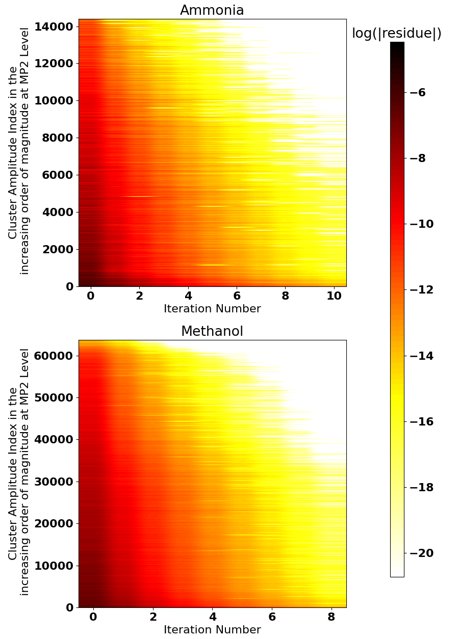
As we mentioned previously in the introduction, the different cluster amplitudes have different time scales in reaching their fixed point solutions, which are taken as the converged values of the amplitudes with a predefined tolerance. In order to show this difference in the relaxation time-scale for different amplitudes, in Fig. 1, we have shown the variation of the absolute residues (defined as the numerator on the right-hand side in Eq. 2) as a function of the iteration step for two different molecules. Note that the residue is a measure of the difference of the amplitudes in successive iterations (see Eq. 2). Here in the vertical axis, we have arranged the first order cluster amplitudes in an increasing order of magnitudes top to bottom, and this is expected to give a fairly good estimate of their relative ordering even after the convergence. Here in the plot, the red colour signifies the larger magnitude of the residue, while the smaller ones are towards white. Note that larger the magnitude of the amplitudes, the larger is the variation of the amplitudes (i.e., a larger magnitude of the residues). Also, note that the larger amplitudes take a longer time to settle. This implies that the residues associated to these larger amplitudes take much higher number of iterations to go below a threshold of tolerance. They are thus the unstable modes of the dynamics. On the other hand, smaller the amplitudes, the residues take fewer iterations to get below the threshold, and thus they are the stable modes in the dynamics. Clearly, there is a difference in the time scale for the large and the small amplitudes to reach their respective fixed points.
In this article, we exploit this difference in their time scale to simplify the convergence procedure. In what follows, we would show that it is possible to restrict the iteration process to determine only the largest amplitudes which have longer relaxation time scale, while the smaller amplitudes would simply be parametrized as the functionals of the previously mentioned large amplitudes. This is the central topic in Synergetics where one deals with the dimensionality reduction in multivariate nonlinear dynamics to work with fewer degrees of freedom. At this stage, let us set the nomenclatures and notations. The large amplitudes that play the the role of unstable modes, and drive the overall iteration process will be termed interchangeably as the driver or the principal amplitudes. Space spanned by these principal amplitudes will be termed as the largest subspace (LS), and the operators corresponding to the principal amplitudes will simply be called as the principal cluster operators. Let us generically denote these principal amplitudes as . Thus the set denotes the collection of all the principal cluster amplitudes which belong to the LS. Let us denote their dimension as . On the other hand, the smaller amplitudes (the stable modes of the dynamics, having a shorter time scale) which supposedly “work under” the principal amplitudes would be referred to as the auxiliary amplitudes. In Synergetics, the principal and auxiliary amplitudes are referred to as the ‘master’ and ‘slave’ variables. The space spanned by the slaved amplitudes will be termed as the smaller subspace (SS). Let us denote the set of the auxiliary amplitudes generically as . The in the subscript stands for ‘small’ to indicate that they are much smaller in magnitude than ’s. The dimension of the smaller subset, denoted by is much larger than : . Note that at this stage, we have not followed any established procedure to distinguish the principal and the auxiliary amplitudes. Rather, the principal amplitudes are taken to be a small fraction (10%-20% of elements having the highest magnitude) of the total nonzero amplitudes. However, a more rigorous choice of the principal amplitudes and the LS can be made based on the information theoretical techniques, or by analysing the Lyapunov exponents arising out of the Jacobian stability matrix. This will be the topic of a future publication. In the current work, by exploiting the difference in the relaxation time scale of the principal and auxiliary amplitudes, we will analytically establish their interdependence. We would also schematically show how an iteration scheme can be built at a much cheaper computational scaling based on the above observations.
III The Circular Causality Relationship between the Principal and Auxiliary Amplitudes:
As discussed previously, the fundamental assumptions of Synergetics dictate that the macroscopic progression of the iteration process is almost entirely governed by the principal cluster amplitudes belonging to LS. As shown in Fig. 1, these principal amplitudes have a longer time scale of relaxation to reach the fixed point solutions. Contrary to that, there is the smaller subspace, SS, which contains all the remaining smaller cluster amplitudes. The variation of the auxiliary amplitudes is suppressed and we can assume that their contribution to the macroscopic dynamics is asymptotically negligible. These auxiliary cluster amplitudes are thus enslaved under the driver amplitudes, and they are thus often termed as ‘slave’ amplitudes. Following the principles of Synergetics and our earlier work, we conjecture that each of the auxiliary amplitudes can be written as a functional of the principal driver amplitudes.
| (1) |
Here small denotes the index of the auxiliary amplitudes and they belong to the smaller subset. Thus . The set denotes the entire group of the principal amplitudes which is a collection of elements. denotes the discrete time step. Assuming that the auxiliary amplitudes have a much faster and suppressed variation compared to the large principal amplitudes which are characterized by slow relaxation time scale to reach the fixed points, we employ an adiabatic decoupling condition such that one may approximate the functional form for each excitation associated with the auxiliary amplitudes. Unlike our previous attempt to numerically simulate via supervised machine learning, in this work, we analytically arrive at a set of equations for each of the auxiliary amplitudes. This is achieved via decoupling the fast and slow relaxing variables, and exploiting the fact that the variation of the auxiliary amplitudes has little effect in the macroscopic features of the iteration dynamics. Thus their subdynamics is asymptotically negligible. This allows us to express each of the auxiliary amplitudes uniquely by alone. Contrary to that, only the principal amplitudes are determined more accurately via the usual algebraic or diagrammatic techniques which allows the feedback of the auxiliary amplitudes , as well as the coupling with other principal amplitudes . Our overall method relies on the adiabatic decoupling of the fast relaxing stable modes from the slow unstable modes via adiabatic decoupling. In what follows, we will demonstrate that the determination of both the principal and auxiliary amplitudes may be done with a tremendous reduction in computational scaling than the conventional solution of the coupled cluster equations. We will elaborate upon both these steps in the subsequent subsections. Here in Fig. 2, we give a bird’s-eye-view of the entire iteration scheme which consists of these two steps connected via what is referred to as the circular causality loop.
We first choose the principal cluster amplitudes from the first order perturbative estimate. At this stage, the choice of the principal amplitudes is made solely based on the magnitude of the first order cluster operators, and the chosen large amplitudes are assumed to span the LS. All the remaining cluster amplitudes with smaller magnitudes are taken to be the auxiliary enslaved variables. While this choice of the principal amplitudes is good enough for all the practical purposes, as mentioned before, this is somewhat ad-hoc and one needs to resort to a more sophisticated technique to pick up the unstable modes. In an ensuing article, we would demonstrate how one may choose the principal amplitudes via the maximization of the mutual information. However, this will not be discussed any further in the present article. The largest amplitudes are then mapped on to the smaller auxiliary amplitudes via step-I using the adiabatic decoupling condition. In the next subsection, we will show that in order to determine the auxiliary amplitudes, only the principal amplitudes are allowed to contribute, while the coupling among the auxiliary amplitudes are switched off. Thus each of the auxiliary amplitudes are written as unique functional of the principal amplitudes. The large driver amplitudes and the auxiliary amplitudes thus obtained via adiabatic decoupling are then allowed to couple to obtain an updated set of principal amplitudes as shown in step-II. This overall feedback mechanism is known as the circular causality loop in Synergetics, which is continued till all the principal amplitudes (and hence the auxiliary amplitudes due to their fixed functional dependence on the principal amplitudes) are converged. In the next subsection, we will discuss both these steps in more detail and show their exact interdependence.
III.1 The Parametrization of the Auxiliary Amplitudes: the Adiabatic Decoupling Condition:
In this subsection, we would elaborate upon the forward mapping in which the auxiliary amplitudes are expressed in terms of the principal amplitudes, as shown by step-I in Fig. 2. Here we borrow heavily from the statistical description of self-organization where many variables coherently “work together” without any external stimuli[14, [Chapter~7]haken2013synergetics]. Let us look at the coupled cluster iteration scheme as a self-organizing system containing various interacting subsystems.
Let us consider the coupled cluster Jacobi iteration scheme:
| (2) |
Here is the cluster operator, is the one and two electron Hamiltonian matrix element. denotes the associated amplitudes with hole-particle excitation structure ‘’. The notation means the composite inside the parenthesis, generated out of the contraction of Hamiltonian and the cluster operator(s) have the hole-particle excitation structure as . At this stage, we have not distinguished between the principal and the auxiliary amplitudes. Thus, is a generalised notation of the hole-particle excitations, which can be either principal or auxiliary amplitudes. is the associated denominator, usually taken to be the Hartree-Fock orbital energy difference. As such, in CC theory, as shown earlier, there is a bunch of amplitudes which enslave subsystems composed of auxiliary amplitudes. In a more generalized case with multiple subsystems, they are separately defined by several groups of non-interacting auxiliary variables which are enslaved under separate interacting groups of the master amplitudes. In the simplest case scenario, the iteration process in CC theory can be viewed as an interplay of two interacting subsystems: one containing the principal amplitudes while the second one contains only the auxiliary slave amplitudes. As shown previously via the circular causality relationship, the master variables (principal amplitudes) determine the dynamics of the slave variables (auxiliary amplitudes), while the updated slave amplitudes pass on their feedback to the master amplitudes without affecting the macroscopic pattern of the overall dynamics. Here we show how enslaved amplitudes are governed solely via the master amplitudes.
As mentioned previously, the amplitudes are grouped into two classes: the principal amplitudes, denoted as , and the auxiliary amplitudes, denoted as {. A general structure of the iteration scheme for different principal amplitudes (necessarily belonging to the largest subset) may be written as:
| (3) |
As before, the notation means the composite inside the parenthesis have the hole-particle excitation structure as . Similarly, the equations for determining the enslaved auxiliary amplitudes, , read as:
| (4) |
Note that till now, the s appearing in the second and third terms on the right hand side of the above equations contain both the principal and auxiliary amplitudes. One may cast the above two equations schematically for the principal and auxiliary amplitudes as:
| (5) |
and,
| (6) |
Here we have extracted out the diagonal contribution from the linear terms, in which the hole-particle excitation in the cluster operator has the same indices as the composite residue. is thus the collection of the Hamiltonian matrix elements associated with the diagonal term, which upon contraction to produces the composite having same hole-particle structure same as . Hence to distinguish this term from the two body matrix element which itself has hole-particle excitation structure as , the former is depicted by the superscript . Here is a general nonlinear function that contains the constant term, and various linear (except diagonal) and all nonlinear terms which arise out of the Baker-Campbell-Hausdorff expansion. Note that Eqs. 5 and 6 have the general structure as:
| (7) |
Here in Eq. 7 is the generalised
notation of the collection of the Hamiltonian matrix
elements, , which accompanies the diagonal terms
in the equations for various ’s.
Note that has opposite sign to that
of which is evident from their leading order
contributions, and is a measure of the damping constant
associated with the relaxation process of .
Here we sketchily analyse the leading order contribution
to the damping constant .
The leading order contribution to in Eqs.
5 and 6 is the difference in
energies involving orbitals of .
Please see the Appendix for the detailed structure of
the Hamiltonian matrix element associated with these
diagonal terms in the orbital basis. Since the inverse of
the damping constant is proportional to the time scale of
relaxation, one may split the amplitudes into slow and fast
relaxing modes by analysing the leading order Hamiltonian
matrix elements.
Note that the principal amplitudes are large in magnitude
and they are labelled by orbitals which are energetically
close. Hence they have smaller damping constants, and
thus they are characterized by a longer time of relaxation
to reach their respective fixed points. On the other hand,
the auxiliary amplitudes are labelled by orbitals which are
energetically well separated. The leading term
contributing to the damping constant, involving the
Hartree-Fock orbital energy difference, appearing in the
equations for , is large. Thus
the auxiliary amplitudes are characterized by larger
damping constant and a shorter time scale of relaxation.
We are now in a position to apply the adiabatic condition
to simplify the working equations. Noting the fact that
the principal and the auxiliary amplitudes exhibit vastly
different time scale of relaxation, and that
the variation of the auxiliary amplitudes are suppressed,
one may invoke an adiabatic approximation by putting
.
Furthermore, as we argued earlier, we assume that the
magnitude of the auxiliary amplitudes, is
much smaller compared to the principal amplitudes:
. As a consequence, we may put
to zero for all values of in the
equations for the auxiliary amplitudes. This allows
us to write down the equations for the auxiliary
amplitudes as
| (8) |
where are put to zero in the nonlinear terms in Eq. 6. Note that the right hand side of Eq. 8 has only and hence no coupling is allowed among the auxiliary cluster amplitudes in their equations.
We can now expand the above equations in terms of explicit contraction between the Hamiltonian matrix elements and the cluster operators which will help us in discerning the scaling associated to each term. The second equation in Eq. 8 may be written explicitly as:
| (9) |
Here has explicitly been written as the Hamiltonian matrix element , which upon contraction with produces the composite that has the same hole-particle excitation as . An explicit expression for is given in the appendix. We reiterate that this term is to be distinguished from the first term inside the parenthesis in the right-hand side of the above equation. Here means the matrix element of Hamiltonian, which has the hole-particle excitation structure as . Note that in Eq. 9, only the principal cluster operators and appear in the right hand side, and there is no term which contains the auxiliary amplitudes. It is interesting to note that the auxiliary amplitudes are not frozen to predefined values; rather they relax in each iteration step via a fixed functional dependence on the principal amplitudes as shown in Eq. 9.
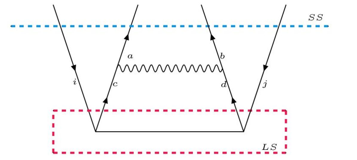

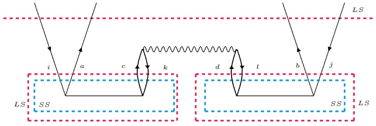
Let us now consider the scaling associated with the construction of the linear and the nonlinear terms in Eq. 9, as shown by term I and II, respectively. The most expensive diagram in the conventional CCSD arises where two particle orbitals contract with the two-body cluster operators. The scaling associated with the construction of this term is . The same term is represented diagrammatically in Fig. 3. Note that according to term-I in Eq. 9, the set of uncontracted indices in Fig. 3 must correspond to the cluster operators belonging to the smaller subspace, and this is generated by the contraction of the Hamiltonian matrix element with the principal cluster operators. Thus and . This term can be generated at a scaling . Note that is only a small fraction (usually 10%-20%, vide infra) of the total number of cluster operators. This leads to an order of magnitude reduction in scaling in constructing the most expensive CC diagram.
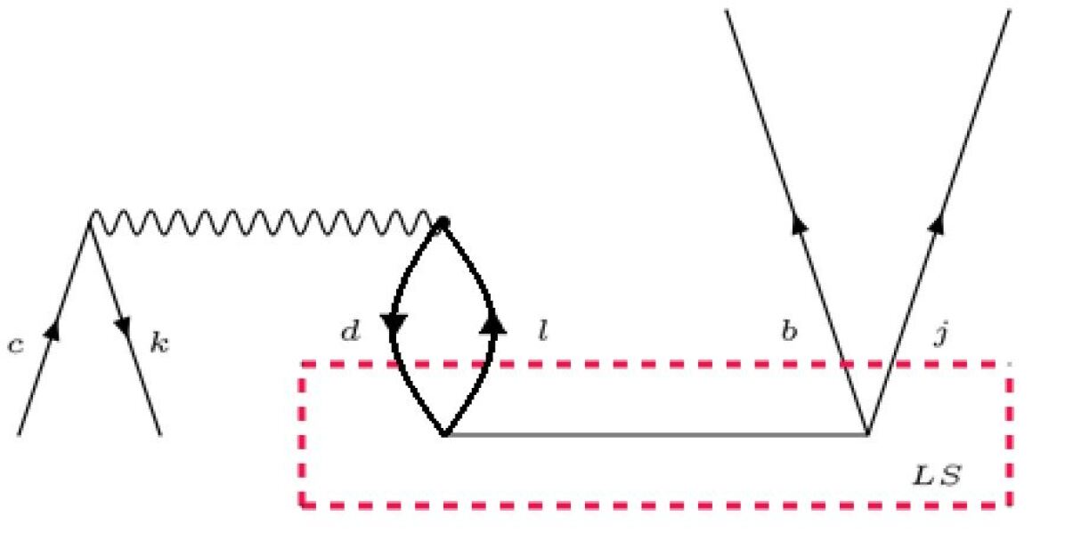
We now turn our attention to the construction of the nonlinear terms as indicated by II in Eq. 9. Let us consider the diagram as shown by Fig. 4a. As it was in the case for the linear term, here also the set of uncontracted indices corresponds to the auxiliary cluster operators. Thus, . This term is generated via the contraction of the Hamiltonian with two principal cluster operators: , and . Like the conventional CC theory, this too can be constructed via an optimal intermediate shown in Fig. 4b. In order to generate this intermediate, one may restrict the pair of orbitals and to unique pair labels that appear in one of the vertices of the principal operators (in the LS). This is a small fraction of terms compared to keeping number of terms in an unrestricted manner. Thus the construction of the intermediate takes matrix operations. Here , which is smaller than . Thus the overall computational scaling to construct the intermediate, , is much smaller than the conventional as required in the conventional CC. The construction of the final diagram via this intermediate and takes the same computational scaling. Thus the overall scaling for the generation of the auxiliary amplitudes are reduced by at least an order of magnitude compared to the conventional CCSD. We now focus on the feedback coupling to determine the principal cluster amplitudes as shown in step II of the circular causality diagram.
III.2 The Feedback coupling: Determination of the principal driver amplitudes:
As we had shown in the earlier section, due to the difference in the time scale, the auxiliary amplitudes can be decoupled from the principal amplitudes by demanding that the variation of the former is suppressed during the iteration process. This, coupled with the elimination of the auxiliary amplitudes from their equations due to their smallness in magnitude, allows us to write the auxiliary amplitudes in terms of the functionals of the principal amplitudes alone. We now focus on the determination of the principal amplitudes. Noting the fact that each auxiliary amplitudes are functionals of the principal amplitudes, one may now rewrite Eq. 5 as:
| (10) |
Here we have explicitly shown that the auxiliary amplitudes appearing in various are functions of the principal amplitudes. Absorbing the diagonal term, one may recast Eq. 3 as:
| (11) |
with
| (12) |
Here, we have explicitly shown the different combinations of the linear and the nonlinear terms that appear with various powers of the principal and auxiliary cluster amplitudes. As we argued above, the auxiliary amplitudes are written explicitly as functional of the principal amplitudes, and they are determined via Eq. 9. Depending on which set of terms are retained in the equations of the principal amplitudes in Eq. 11, we have devised two schemes having different levels of sophistication, as discussed below.
In scheme-I, we have kept all the terms (I-VI) in Eq. 11, and we will refer this scheme as AD-CC (Scheme-I). This thus introduces complete feedback of the auxiliary amplitudes to the equations for the principal amplitudes, and hence the principal amplitudes are determined exactly. On the other hand, since the auxiliary amplitudes are much smaller in magnitude compared to the principal amplitudes, one may selectively include only those terms in Eq. 11 where the auxiliary amplitudes are kept only up to the linear power. This implies that all the nonlinear terms which include auxiliary amplitudes may safely be neglected. Thus in AD-CC (Scheme-II), we have retained terms (I-IV), and have neglected terms (V-VI) in Eq. 11 for determining the principal cluster amplitudes. We will show in the next section that although this may seem to be a rather drastic approximation, the accuracy of the results does not deteriorate much compared to scheme-I. In fact, AD-CC (Scheme-II) may be chosen as an excellent cost effective way to solve CC theory without scarifying the accuracy significantly. It will also be pretty evident that the results are systematically improvable by going from scheme-II to scheme-I, since the latter has a more complete expression for the principal amplitudes. One may also design a mid-way scheme where all the terms (I-V) are included and only term VI is neglected in Eq. 11. However, in the present work, we have not considered this alternative. Below, we discuss the computational scaling for the determination of the principal amplitudes via both the schemes.
Note that in both schemes-I and scheme-II, both the linear terms, II and III, are included in Eq. 11. This implies that both the principal and the auxiliary cluster operators contract to the Hamiltonian to generate a composite structure where the uncontracted indices may take only those values which together characterize a principal cluster operator. This is diagrammatically shown via the most expensive CC diagram in Fig. 5. Note that in Fig. 5, unlike Fig. 3, the set of uncontracted indices necessarily characterize a principal cluster operator, whereas the horizontal solid line can be both principal and auxiliary cluster operators. Since the uncontracted indices are restricted to the LS elements, one trivially can construct this term at a scaling of . Although the diagram shown in Fig. 5 is superficially same as that of Fig. 3, note that they have different interpretations in two different contexts.
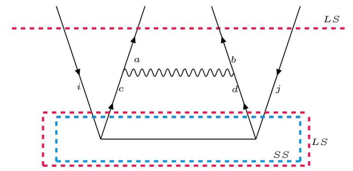
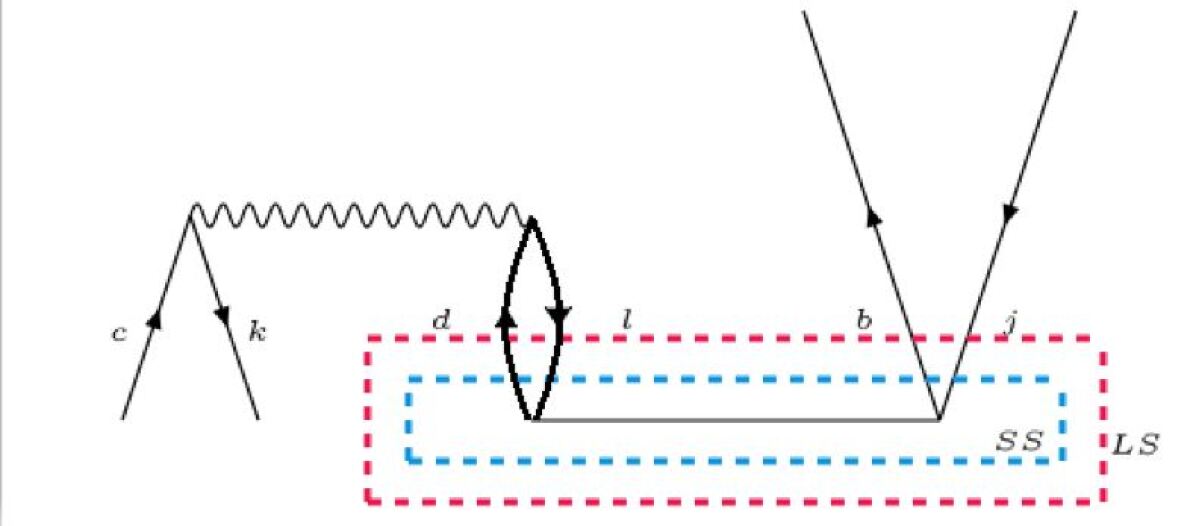
We now turn our attention to analyse the scaling of the nonlinear diagrams in Eq. 11. One may again construct diagrams of similar topology like those appearing in Fig. 4a, and interpret it in the context of Eq. 11. Here we analyse a diagram as shown in Fig. 6a, having similar topology to that of Fig. 4a. Note that like the linear term, the set of uncontracted index can take only those elements which characterize a principal cluster amplitude. However, in AD-CC (scheme-I), the cluster operators and can be both principal and auxiliary operators as evident from Eq. 11. Since the set of uncontracted indices belong to LS, in order to construct the intermediate as shown in Fig 6b, one may restrict the pair of orbitals and to unique pair labels which appear in one of the vertices of the principal cluster operators. Note that the orbitals and can take up any value from the entire set of occupied and unoccupied orbitals respectively. Thus to construct the intermediate, one needs to perform matrix operations, which is less than matrix operations needed to construct the same intermediate in the conventional CC theory. The next step to construct the entire diagram takes computational scaling.
On the other hand, in AD-CC (scheme-II), the cluster operators and can only be the principal cluster operators. That implies that the intermediate, as shown in Fig 6b, can be constructed with a computational scaling of . Note that this is one to two order of magnitude reduction compared to the conventional scaling necessary to construct the diagram. In the next section, we will present a few prototypical numerical results to demonstrate the efficacy of both the schemes. We will also demonstrate the relative scaling of our schemes for the construction of the linear and nonlinear terms that appear in the forward mapping (step-I, Fig. 2) and backward mapping (step-II, Fig. 2) compared to the conventional CCD scheme.
IV Results and Discussion
In this section, we demonstrate the efficacy of the AD-CC (scheme-I/II) with a number of molecular systems. As the proof of the concept, we will restrict our applications to adiabatically decoupled CCD (AD-CCD) theory, although the generalization to include singles or triples and higher excitations is fairly straightforward. All the calculations were done using our in-house CC codes, and the convergence threshold for all the calculations was set to be . No DIIS routine was used to accelerate the calculations although doing so is fairly straightforward.
| Ammonia () Asymmetric | Methanol () (slightly symmetric) | Ethene () (highly symmetric) | ||||||||||
| LS Size (% of Non zero elements) | 10 | 15 | 20 | 25 | 10 | 15 | 20 | 25 | 10 | 15 | 20 | 25 |
| 95 | 96 | 98 | 99 | 266 | 274 | 279 | 282 | 176 | 209 | 225 | 234 | |
| Linear term construction (Eq. 9, term-I, Fig. 3) AD-CCD:CCD = | 0.1 | 0.15 | 0.2 | 0.25 | 0.05 | 0.075 | 0.1 | 0.125 | 0.01 | 0.015 | 0.02 | 0.025 |
| Linear term construction (Eq. 11, term-II +III, Fig. 5) AD-CCD:CCD = | 0.1 | 0.15 | 0.2 | 0.25 | 0.05 | 0.075 | 0.1 | 0.125 | 0.01 | 0.015 | 0.02 | 0.025 |
| Intermediate term construction (for term-II in Eq. 9; Fig. 4b) AD-CCD:CCD = | 0.08 | 0.12 | 0.163 | 0.206 | 0.037 | 0.0573 | 0.077 | 0.0975 | 0.0055 | 0.01 | 0.014 | 0.0183 |
| Intermediate term construction (for terms-IV+V+VI in Eq. 11; Fig. 6b) AD-CCD (Scheme-I):CCD: | 0.79 | 0.8 | 0.816 | 0.825 | 0.74 | 0.76 | 0.773 | 0.78 | 0.55 | 0.653 | 0.70 | 0.73 |
| Intermediate term construction (for term-IV in Eq. 11; Fig. 6b) AD-CCD (Scheme-II):CCD = | 0.08 | 0.12 | 0.163 | 0.206 | 0.037 | 0.057 | 0.077 | 0.0975 | 0.0055 | 0.01 | 0.014 | 0.018 |
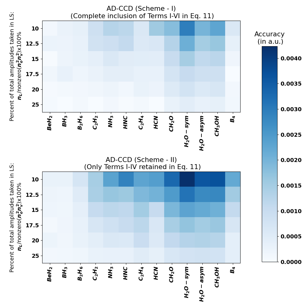
In Fig. 7, we have demonstrated the accuracy of our models for a few molecular systems with varied degree of complexity and size. In the vertical axis, we plot the dimension of the largest subset, which is chosen to vary from 10% to 25% of the total nonzero cluster amplitudes. We reiterate once again that the choice of the LS is somewhat not very elegant, although for all the practical purposes, this is fairly accurate. In Fig. 7, the colour coding of the individual boxes represent the difference of AD-CCD schemes from the canonical CCD calculations. The darker shades imply a larger deviation, while the lighter shades imply a smaller difference.
The upper panel of Fig. 7 shows the accuracy of a few molecules in their equilibrium and away from equilibrium geometries in cc-pVDZ basis in AD-CCD scheme-I, while the lower panel shows the accuracy for scheme-II. Clearly, for all the molecules under consideration, the AD-CCD (scheme-I) shows sub milliHartree () accuracy compared to the conventional CCD with the LS chosen to be the largest 15% of the total cluster amplitudes. The method, as expected, shows a systematic improvement in accuracy as one includes more elements in the LS. With the LS dimension of 20% of the total cluster amplitudes and above, the method, on an average, shows accuracy of the order of 0.1 . Since the AC-CCD (scheme-II) includes an incomplete coupling of the auxiliary amplitudes in the equations for the principal amplitudes, one expects somewhat less accuracy, particularly with smaller size of the LS. This is clearly evident that one needs to increase the LS dimension to 20% to achieve a sub- accuracy in AD-CCD (scheme-II). Nonetheless, scheme-II shows, on an average, deviation of 0.5 with the LS taken to be the 20% of the total number of nonzero cluster amplitudes. On the other hand, AD-CCD (scheme-I) requires 15% of the total nonzero cluster amplitudes to achieve a similar accuracy.
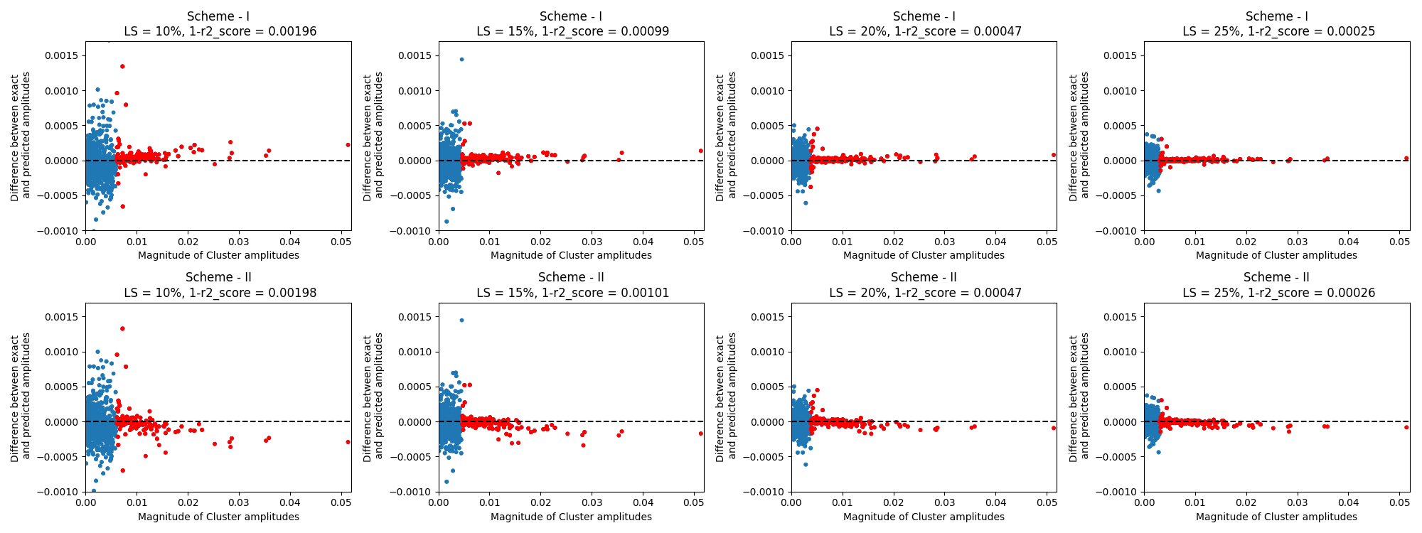
In order to demonstrate the exactness of the cluster amplitudes, in Fig. 8, we have plotted the difference of the exact CCD amplitudes and those predicted via Eqs. 9 and 11 for water molecule at equilibrium in cc-pVDZ basis. The red dots are the principal amplitudes obtained via Eq. 11, while the blue dots signify the auxiliary cluster amplitudes obtained from Eq. 9. Clearly, the smaller amplitudes get more and more accurate as one increases the LS dimension. This in turn results in accurate prediction of the principal amplitudes as well, since the auxiliary amplitudes provide the feedback coupling to the principal amplitudes via Eq. 11. It is to be noted that with increase in the LS dimension, there is a systematic improvement of the accuracy of the predicted cluster amplitudes with the overall R2 score of 0.99804 at 10% to 0.99975 at 25% with AD-CCD (scheme-I). The approximated AD-CCD (scheme-II) also shows quite a similar trend (R2 score=0.99974 at 25%), although it is marginally less accurate with smaller dimension of the LS (R2 score=0.99802 at 10%). This is quite expected as scheme-II uses a drastically approximated equation to determine the principal amplitudes where all the nonlinear terms containing the auxiliary amplitudes are neglected. However, with increase in the LS dimension, both the schemes tend to produce similar results as shown over a number of molecular applications in Fig. 7. We reiterate that the remarkable accuracy of AD-CCD, scheme-I in particular, has been achieved with an order of magnitude reduction in computational scaling which will be demonstrated below.
Lastly, we turn our attention to demonstrate the reduction in computational scaling of both the schemes over the conventional CCD. We would be presenting with three different molecular systems having varied degrees of complexity. In Table 1, we have presented the ratio of the computational scaling required for the forward and backward mappings (step-I and step-II, of Fig. 2) for both the schemes to that of the conventional CCD in order to construct the most expensive linear diagram (and the intermediates to the nonlinear diagrams). The rate determining step to the conventional CCD calculations is the construction of the linear diagram where two particle orbitals contract. The scaling associated to this diagram is . Construction of the diagram having same topological structure in both the forward mapping and the feedback coupling scales as . For the highly distorted molecule without any symmetry, the dimension of the LS, , is at max taken to be 10-25% of the total (nonzero) cluster amplitudes for sub accuracy. This leads to at least 75%-90% reduction in computational scaling for the construction of the most expensive CCD diagram which has two particle contraction. We now analyse the computational cost associated with the construction of the intermediates, which in conventional CCD scales as . For AD-CCD (scheme-I), as we have shown in Fig. 6a, we have a lower scaling of , where is the number of unique excitation vertex that appears in the two-body principal cluster operators in the LS. The variation of is shown in Table 1 for different choices of the LS dimension and for different molecules. Clearly, varies sub-linearly with the increase in LS dimension, . Usually, is about 70-80% of . Thus, the construction of the intermediate in Fig. 6a takes computational scaling of about . For AD-CCD (scheme-II), on the other hand, allows only the principal amplitudes in the nonlinear term of the feedback coupling (step-II of Fig. 2). Thus, it further reduces the computational scaling to , which is only about 8-20% of . However, as evident from Fig. 7, this does not deteriorate the accuracy of AD-CCD (scheme-II), particularly with a conservative choice of the LS. We should note that for AD-CCD (scheme-I), in a small basis set, the scaling required for the construction of the intermediate for the nonlinear term is often comparable to the computational scaling required to construct the linear diagram with two particle contraction. On the other hand, in large basis sets, the construction of the linear diagram is the rate determining step. However, we reiterate that in our AD-CCD schemes, the scaling for the construction of this is drastically reduced by 70-80%.
V Conclusion and Future Outlook
In this article, we had developed a novel variant of an approximated CC theory where the solution of two sets of the cluster amplitudes are decoupled. The method relies upon an adiabatic approximation where the fast relaxing stable amplitudes are decoupled and expressed as fixed functionals of the slow moving unstable amplitudes. The principal amplitudes, which are the unstable modes of the iteration dynamics, are determined accurately via exact CC equations that include the coupling of all unstable amplitudes and a feedback coupling of the stable auxiliary amplitudes. Two approximated schemes have been proposed which differ in the level of the inclusion of the nonlinear terms containing the auxiliary amplitudes. As a proof of the concept, we have included only the double excitations in our applications. Both the resulting schemes of AD-CCD have been applied to a number of molecules in their equilibrium and away from equilibrium geometries, and they show remarkable accuracy compared to the conventional CCD. While the typical accuracy of the methods depend on the dimension of the chosen LS, a conservative choice of the LS leads to the results which is accurate up to the order of one hundredth of a . This is achieved with a computational scaling of the order of 10%-25% of the typical scaling of CCD, at worst.
While the current choice of the LS is fairly general and works for all practical purposes, this is not the optimal choice by any means. One may rely upon Lyapunov stability analysis or information theoretic techniques to choose the optimal LS and reduce the computational scaling even further. Moreover, a generalization to the current work to include triples and higher excitations is straightforward, and will be subject to one of our forthcoming publications.
VI Acknowledgments
The authors thank Mr. Anish Chakraborty, IIT Bombay, for many stimulating discussions about the structure of the program. RM acknowledges the financial support from Industrial Research and Consultancy Centre, IIT Bombay, and Science and Engineering Research Board, Government of India, for financial support.
Data Availability
The data is available upon reasonable request to the corresponding author.
References
- C̆íz̆ek [1966] J. C̆íz̆ek, J. Chem. Phys. 45, 4256 (1966).
- C̆íz̆ek [1969] J. C̆íz̆ek, Adv. Chem. Phys. 14, 35 (1969).
- Čížek and Paldus [1971] J. Čížek and J. Paldus, Int. J. Quantum Chem. 5, 359 (1971).
- Bartlett and Musiał [2007] R. J. Bartlett and M. Musiał, Reviews of Modern Physics 79, 291 (2007).
- Szakács and Surján [2008a] P. Szakács and P. R. Surján, 43, 314 (2008a).
- Szakács and Surján [2008b] P. Szakács and P. R. Surján, Int. J. Quantum Chem. 108, 2043 (2008b).
- Maitra and Nakajima [2017] R. Maitra and T. Nakajima, J. Chem. Phys. 147, 204108 (2017).
- Maitra, Akinaga, and Nakajima [2017] R. Maitra, Y. Akinaga, and T. Nakajima, J. Chem. Phys. 147, 074103 (2017).
- Tribedi, Chakraborty, and Maitra [2020] S. Tribedi, A. Chakraborty, and R. Maitra, Journal of Chemical Theory and Computation 16, 6317–6328 (2020).
- Feigenbaum [1978] M. J. Feigenbaum, Journal of statistical physics 19, 25 (1978).
- Agarawal, Chakraborty, and Maitra [2020] V. Agarawal, A. Chakraborty, and R. Maitra, The Journal of Chemical Physics 153, 084113 (2020).
- Haken [1989] H. Haken, Rep. Prog. Phys. 52, 515 (1989).
- Haken and Wunderlin [1982] H. Haken and A. Wunderlin, Z. Phys. B 47, 179 (1982).
- Haken [1983] H. Haken, “Nonlinear equations. the slaving principle,” in Advanced Synergetics: Instability Hierarchies of Self-Organizing Systems and Devices (Springer Berlin Heidelberg, Berlin, Heidelberg, 1983) pp. 187–221.
- Pedregosa et al. [2011] F. Pedregosa, G. Varoquaux, A. Gramfort, V. Michel, B. Thirion, O. Grisel, M. Blondel, P. Prettenhofer, R. Weiss, V. Dubourg, J. Vanderplas, A. Passos, D. Cournapeau, M. Brucher, M. Perrot, and E. Duchesnay, Journal of Machine Learning Research 12, 2825 (2011).
- Agarawal et al. [2021] V. Agarawal, S. Roy, A. Chakraborty, and R. Maitra, The Journal of Chemical Physics 154, 044110 (2021).
- Haken [2013] H. Haken, Synergetics: Introduction and advanced topics (Springer Science & Business Media, 2013).
VII APPENDIX:
| (13) |