ergm 4: New Features

Abstract

The ergm package supports the statistical analysis and simulation of network data. It anchors the statnet suite of packages for network analysis in R introduced in a special issue in Journal of Statistical Software in 2008. This article provides an overview of the new functionality in the 2021 release of ergm version 4. These include more flexible handling of nodal covariates, term operators that extend and simplify model specification, new models for networks with valued edges, improved handling of constraints on the sample space of networks, and estimation with missing edge data. We also identify the new packages in the statnet suite that extend ergm’s functionality to other network data types and structural features and the robust set of online resources that support the statnet development process and applications.

Keywords statistical software  $\cdot$ statnet  $\cdot$ ERGM  $\cdot$ exponential-family random graph models  $\cdot$ valued networks

1 Introduction

The statnet suite of packages for R (R Core Team, 2021) was first introduced in 2008, in volume 24 of Journal of Statistical Software, a special issue devoted to statnet. Together, these packages, which had already gone through the maturing process of multiple releases, provided an integrated framework for the statistical analysis of network data: from data storage and manipulation, to visualization, estimation and simulation. Since that time the existing packages have undergone continual updates to improve and add capabilities, and many new packages have been added to extend the range of network data that can be modeled (e.g., dynamic, valued, sampled, multilevel). It is the ergm package, however, that provides the statistical foundation for all of the other modeling packages in the statnet suite. Version 4 of ergm, released in 2021, is a major upgrade, representing more than a decade of changes and improvements since (Hunter, Handcock, et al., 2008). This paper describes the many updates to the functionality of the package of interest to end users. It is a companion to (Krivitsky et al., 2022), which discusses computational improvements in ergm version 4.

The exponential-family random graph model (ERGM) is a general statistical framework for modeling the probability of a link (or tie) between nodes in a network. It is implemented by the ergm package and most of its related packages in the statnet suite. We consider networks over a set of nodes $N=\{1,2,\dotsc,n\}$. If $\mathbb{Y}\subseteq N\times N$ denotes a set of potential pairwise relationships among them, a binary network sample space can be regarded as $\mathcal{Y}\subseteq 2^{\mathbb{Y}}$, a subset of the power set of potential relationships. More generally, we can define $\mathbb{S}$ to be a (possibly multivariate) set of possible relationship values. Then, the sample space $\mathcal{Y}\subseteq\mathbb{S}^{\mathbb{Y}}$ is a set whose elements are of the form $\{Y\!_{i,j}:{{(i,j)}\in\mathbb{Y}}\}$, where each $Y\!_{i,j}$, which we will call a dyad, maps the node pair ${{(i,j)}\in\mathbb{Y}}$ into $\mathbb{S}$ and denotes the value of the relationship of ${{(i,j)}\in\mathbb{Y}}$.

We begin by briefly presenting the fully general ERGM framework, referring interested readers to Schweinberger et al. (2020) for additional technical details. A random network $\mathbf{Y}$ is distributed according to an ERGM, written $\mathbf{Y}\sim\operatorname{ERGM}_{\mathcal{Y},h,\bm{\eta},\mathbf{g}}({\bm{\theta}})$, if

$$\operatorname{Pr}_{{\bm{\theta}},\mathcal{Y},h,\bm{\eta},\mathbf{g}}(\mathbf{Y}=\mathbf{y})=\frac{h(\mathbf{y})\exp\{\bm{\eta}({\bm{\theta}})^{\top}\mathbf{g}(\mathbf{y})\}}{\kappa_{h,\bm{\eta},\mathbf{g}}({\bm{\theta}},\mathcal{Y})},\ {\mathbf{y}\in\mathcal{Y}}.$$ (1)

In Equation (1), $\mathcal{Y}$ is the sample space of networks; ${\bm{\theta}}$ is a $q$-dimensional parameter vector; $h(\mathbf{y})$ is a reference measure, typically a constant in the case of binary ERGMs; $\bm{\eta}$ is a mapping from ${\bm{\theta}}$ to the $p$-vector of canonical parameters, a linear mapping in non-curved ERGMs, and commonly an identity mapping $\bm{\eta}({\bm{\theta}})\equiv{\bm{\theta}}$; $\mathbf{g}$ is a $p$-vector of sufficient statistics; and $\kappa_{h,\bm{\eta},\mathbf{g}}({\bm{\theta}},\mathcal{Y})$ is the normalizer given by $\sum_{{\mathbf{y}^{\prime}\in\mathcal{Y}}}h(\mathbf{y}^{\prime})\exp\{\bm{\eta}({\bm{\theta}})^{\top}\mathbf{g}(\mathbf{y}^{\prime})\}$, which is often intractable for models that seek to reproduce the dependence across ties induced by social effects such as triadic closure. The natural parameter space of the model is $\bm{\Theta}_{\text{N}}\stackrel{{\scriptstyle\text{def}}}{{=}}\{{\bm{\theta}}:\kappa_{h,\bm{\eta},\mathbf{g}}({\bm{\theta}},\mathcal{Y})<\infty\}$.

For a particular network application, one would typically employ a special case of the fully general Equation (1). For instance, for binary ERGMs we typically define $h(\mathbf{y})$ to be a constant, as discussed in Section 6.1, in which case the sufficient statistics can be thought of as modifying a uniform baseline distribution over the potentially observable networks. Many of the features of ergm and the related packages that comprise the statnet suite address the statistical complications that arise from modeling network data using special cases of the ERGM in Equation (1).

In particular, the statistical framework implemented in ergm is computationally intensive for models that specify dyadic dependence, when $\operatorname{Pr}_{{\bm{\theta}},\mathcal{Y},h,\bm{\eta},\mathbf{g}}(\mathbf{Y}=\mathbf{y})$ cannot be decomposed into a product of simple functions of $y_{i,j}$. In this case, the package relies on a central Markov chain Monte Carlo (MCMC) algorithm for estimation and simulation, along with maximum pseudo-likelihood estimation, contrastive divergence, and simulated annealing in some contexts. Substantial improvements have been made to all of these algorithms, producing efficiency and speed gains of up to several orders of magnitude (Krivitsky et al., 2022). This article describes the most important new capabilities that have been added to ergm and its related packages since volume 24 of Journal of Statistical Software appeared in 2008. This includes both the capabilities introduced in the version 4 release itself and in releases 2.2.0–3.10.4, which postdate the JoSS volume. Versions in which each new capability was introduced can be obtained by running news(package="ergm").

In the examples throughout the article, we assume the reader is familiar with the basic syntax and features of ergm included in the 2008 JoSS volume. In some cases we demonstrate new, more general, functionality by comparison, using the old syntax and the new to produce the same result, then moving on with the new syntax to demonstrate the additional utilities.

The source code for the latest version of the ergm package, along with the LICENSE information under GPL-3, is available at https://github.com/statnet/ergm.

2 Extension packages in the statnet suite

The statistical models supported by the statnet suite have been extended by a growing number of new packages that provide additional functionality in the general ERGM framework. While the focus of this article is the base ergm package, in this section we provide a brief overview of the extension packages and their specific applications. Open source package development is on GitHub under the statnet organization. Online tutorials, found at https://github.com/statnet/Workshops/wiki, exist for ergm and many of these extension packages, and most packages also include extended vignettes. Some of the key extension packages, and the resources that support them, include:

Building custom terms for models

One of the unique aspects of this modeling framework is that each network statistic in an ERGM requires a specialized algorithm for computing the value of the statistic from the data. The ergm package has over 150 of the most common terms encoded—see vignette('ergm-term-crossRef') or help("ergmTerm") for the full list—but the existing terms are a small subset of the possible terms one can use in an ERGM. For those who need a custom term, the package ergm.userterms (Hunter et al., 2013) is designed to simplify the process of coding up new terms for use in ERG model specification. Online workshop materials provide an overview of the process, and demonstrate the use of this package (Hunter & Goodreau, 2019).

Modeling temporal (dynamic) network data

The statnet suite contains several packages that provide a robust framework for storing, visualizing, describing and modeling temporal network data: The networkDynamic package extends network to provide data storage and management utilities, the tsna package extends sna (Butts, 2008) to provide descriptive statistics for network objects that change over time, the ndtv package provides a wide range of utilities for visualizing dynamic networks and saving both static and animated output in standard formats, and tergm extends ergm to fit the class of separable temporal ERGMs, from both sampled and fully observed network data (Krivitsky & Handcock, 2014). There are two online workshops that demonstrate these tools: one that demonstrates a typical workflow from data inspection to temporal modeling (Morris & Krivitsky, 2015), and another that focuses on descriptive analyses and visualization (Bender-deMoll, 2016).

Modeling valued edges

The ergm itself contains a framework for modeling real-valued edges (see Section 6 and Section 4). Several other packages provide specialized components for specific types of valued edges: ergm.count for counts, ergm.rank for ordered categories. The relevant theory supporting these packages may be found in Krivitsky (2012) and Krivitsky & Butts (2017), respectively. latentnet for latent space models also supports non-binary responses, although in a somewhat different manner (Krivitsky et al., 2009; Krivitsky & Handcock, 2008). Package vignettes and online workshop materials provide an overview of the theory, and demonstrate the use of these packages (Krivitsky & Butts, 2019).

Working with egocentrically sampled network data

In the social and health sciences, egocentrically sampled network data is the most common form of data available, because it can be collected using standard sample survey methods. The ergm.ego package provides methods for estimating ERGMs from egocentrically sampled network data, with a principled framework for statistical inference. The theory and an application of these methods may be found in Krivitsky & Morris (2017). Online workshop materials provide an overview of the framework and demonstrate the use of the package (Morris & Krivitsky, 2019).

Multimode, multilayer, and multilevel networks

In the social sciences, it is increasingly common to collect and fit ERGMs on data on multiple relationship types (Krivitsky et al., 2020; Wang, 2012) and ensembles of networks (Slaughter & Koehly, 2016). These capabilities are implemented in an extension package ergm.multi. We refer the reader to the package manual and workshops for further information.

Modeling diffusion and epidemics on networks

One of the most active application areas for ERGMs and TERGMs is in the field of epidemic modeling. The EpiModel package is built on the statnet platform, and provides a unique set of tools for statistically principled modeling of epidemics on networks (Jenness et al., 2018). A robust set of online training materials is available at the EpiModel website.

3 Enhanced handling of nodal covariates

Version 4 of ergm standardizes and provides greater flexibility for handling covariates used by terms in an ERGM. In particular, these covariates can be modified “on-the-fly” during model specification. A vignette called nodal_attributes is included in the package and illustrates some of the new capabilities.

Here, we describe some of these enhancements using ergm’s faux.mesa.high dataset, a simulated in-school friendship network based on data collected on 205 students. We will focus on the Grade attribute, an ordinal categorical variable with values 7 through 12 that can be accessed via the %v% operator:

data(faux.mesa.high)

(faux.mesa.high %v% "Grade")[1:20]  # Look at first 20 nodes' (students') grade levels

##  [1]  7  7 11  8 10 10  8 11  9  9  9 11  9 11  8 10 10  7 10  7

Grade level is typical of the kind of covariate used to model selective mixing in social networks: different hypotheses lead to different model specifications. ergm 4 provides greater flexibility than earlier versions of ergm to easily define and explore different specifications.

We will sometimes call summary() and other times call ergm() to demonstrate the functionality and output below.

3.1 Transformations of covariates

It is sometimes desirable to specify a transformation of a nodal attribute as a covariate in a model term. Most ergm terms now support a new user interface, inspired by purrr (Henry & Wickham, 2020), to specify transformations on one or more nodal attributes. Terms typically use this new interface via arguments called attr, attrs, by, or on; the interpretation of the argument depends on its type:

character string

Extract the vertex attribute with this name.

character vector of length greater than 1

Extract the vertex attributes and paste them together, separated by dots if the term expects categorical attributes and (typically) combine into a covariate matrix if it expects quantitative attributes.

function

The function is called on the network on the left-hand side of the main ergm formula and is expected to return a vector or matrix of appropriate dimension. (Shorter vectors and matrix columns will be recycled as needed.)

formula

Borrowing the interface from tidyverse, the expression on the right hand side of the formula is evaluated in an environment of the vertex attributes of the network, expected to return a vector or matrix of appropriate dimension. (Shorter vectors and matrix columns will be recycled as needed.) Within this expression, the network itself is accessible as either . or .nw.

AsIs object created by I()

Use as is, checking only for correct length and type, with optional attribute "name" providing the predictor’s name.

For instance, here are three ways to compute the value of

$$g(\mathbf{y})=\sum_{{{(i,j)}\in\mathbb{Y}}}y_{i,j}(\text{Grade}_{i}+\text{Grade}_{j}),$$

which in an ERGM may be interpreted as the linear effect of grade on overall activity of an actor:

summary(faux.mesa.high ~ nodecov("Grade")                    # String

                       + nodecov(~Grade)                     # Formula

                       + nodecov(function(nw) nw%v%"Grade")) # Function

##        nodecov.Grade        nodecov.Grade nodecov.nw%v%"Grade"
##                 3491                 3491                 3491

Here is a more complicated formula-based use of nodecov, where the first statistic is

$$g(\mathbf{y})=\sum_{{{(i,j)}\in\mathbb{Y}}}y_{i,j}\left(\frac{\left|\text{Grade}_{i}-\overline{\text{Grade}}\right|}{n}+\frac{\left|\text{Grade}_{j}-\overline{\text{Grade}}\right|}{n}\right),$$

and $n$ is the number of nodes, i.e., the network size, of the network:

summary(faux.mesa.high ~ nodecov(~abs(Grade - mean(Grade)) / network.size(.))

                       + nodecov(~(Grade - mean(Grade)) / network.size(.)))

## nodecov.abs(Grade-mean(Grade))/network.size(.)    nodecov.(Grade-mean(Grade))/network.size(.)
##                                      2.8565140                                     -0.2637716

The non-zero output of the second statistic above, which omits the absolute value, may be counterintuitive if you are expecting it to return the sample mean grade, $\overline{\text{Grade}}$. Node factor statistics, however, are not the sample mean grade: each node is not counted exactly once, but rather the number of cases it contributes is equal to its degree.

Taking advantage of nodecov’s new ability to take matrix-valued arguments, we might also evaluate a polynomial effect of Grade, as in the following quadratic example:

coef(summary(ergm(faux.mesa.high ~ edges + nodecov(~cbind(Grade, Grade2=Grade^2)))))

##                  Estimate Std. Error MCMC %   z value     Pr(>|z|)
## edges           8.7297963 3.52880543      0  2.473867 0.0133659343
## nodecov.Grade  -1.4597723 0.39614405      0 -3.684953 0.0002287445
## nodecov.Grade2  0.0768836 0.02154632      0  3.568294 0.0003593133

In the code above, the column for Grade^2 is explicitly named Grade2 whereas the column for Grade is named implicitly by R itself. Omitting the name for a column not otherwise named by R would result in a warning, as it is good practice to name all variables in the model.

Alternatively, we can use stats::poly for orthogonal polynomials. Here, the test for significance of the quadratic term is identical to the non-orthogonal example, up to rounding error (though the estimate is different given the orthogonal specification):

coef(summary(ergm(faux.mesa.high ~ edges + nodecov(~poly(Grade, 2)))))

##                          Estimate Std. Error MCMC %    z value     Pr(>|z|)
## edges                   -4.662459 0.07309281      0 -63.788207 0.0000000000
## nodecov.poly(Grade,2).1 -1.207241 0.68018706      0  -1.774866 0.0759199607
## nodecov.poly(Grade,2).2  2.512615 0.70416949      0   3.568196 0.0003594477

We can even pass a nodal covariate that is not already contained in the network object. This example randomly generates a binary-valued nodal covariate and sets its name attribute to be used as a label:

set.seed(123)  # Make exact output reproducible

randomcov <- structure(rbinom(network.size(faux.mesa.high), 1, 0.5), name = "random")

summary(faux.mesa.high ~ nodefactor(I(randomcov)))

## nodefactor.random.1
##                 199

This syntax therefore allows for simulation or estimation of models with inputs taken from arbitrary R functions or data sources, facilitating the incorporation of ERGMs into more general tool chains.

3.2 Coding categorical attributes

For model terms that use categorical attributes, ergm 4 has extended the methods for selecting and/or transforming levels via the use of the argument levels. Some terms, such as the sender and receiver statistics of the $p_{1}$ model (Holland & Leinhardt, 1981) and the corresponding sociality statistics for undirected networks, treat the node labels themselves as a categorical attribute. These terms use the nodes= argument, rather than the levels= argument, to select a subset of the nodes.

Typically, levels or nodes has a default that is sensible for the term in question. (Information about the defaults of a term [name] may be obtained by typing help("[name]-ergmTerm") or ergmTerm?[name].) Interpretation of the possible values of the levels and nodes arguments is available by typing help(nodal_attributes). This interpretation is summarized as follows:

AsIs object created by I()

Use the given level, list of levels, or vector of levels as is.

numeric or logical vector

Used for indexing of a list of all possible levels (typically, unique values of the attribute) in default order (typically lexicographic). Logical values are recycled to the length of the vector indexed. In particular, levels=TRUE retains all levels. Negative values exclude. To specify numeric or logical levels literally, wrap them in I().

NULL

Retain all possible levels; usually equivalent to passing TRUE.

character vector

Use the given level(s) as is.

function

The function is called in an environment in which the network itself is accessible as .nw, the list of unique values of the attribute as . or as .levels, and the attribute vector itself as .attr. Its return value is interpreted as above.

formula

The expression on the right hand side of the formula is evaluated in an environment in which the network itself is accessible as .nw, the list of unique values of the attribute as . or as .levels, and the attribute vector itself as .attr. Its return value is interpreted as above.

predefined function

For convenience, a number of useful functions have been predefined. LARGEST, which refers to the most frequent category, so, say, to set such a category as the baseline, pass levels=-LARGEST. LARGEST(n) will refer to the n largest categories. SMALLEST works analogously, and ties in frequencies are broken arbitrarily.

Returning to the faux.mesa.high example, we may treat Grade as a categorical variable even though its values are numeric. We see that Grade has six levels, numbered from 7 to 12:

table(faux.mesa.high %v% "Grade")

##
##  7  8  9 10 11 12
## 62 40 42 25 24 12

We may exclude the three smallest levels or, equivalently, include levels 7, 8, and 9. Below are five of the myriad ways to do this in the context of computing basic categorical effects on node activity, implemented by nodefactor. In the second expression, I() is necessary so that 7:9 is not treated as a vector of indices.

summary(faux.mesa.high ~ nodefactor(~Grade, levels = -SMALLEST(3)))

## nodefactor.Grade.7 nodefactor.Grade.8 nodefactor.Grade.9
##                153                 75                 65

summary(faux.mesa.high ~ nodefactor(~Grade, levels = I(7:9)))

## nodefactor.Grade.7 nodefactor.Grade.8 nodefactor.Grade.9
##                153                 75                 65

summary(faux.mesa.high ~ nodefactor(~Grade, levels = c("7", "8", "9")))

## nodefactor.Grade.7 nodefactor.Grade.8 nodefactor.Grade.9
##                153                 75                 65

summary(faux.mesa.high ~ nodefactor("Grade", levels = function(a) a %in% 7:9))

## nodefactor.Grade.7 nodefactor.Grade.8 nodefactor.Grade.9
##                153                 75                 65

summary(faux.mesa.high ~ nodefactor("Grade", levels = ~. %in% 7:9))

## nodefactor.Grade.7 nodefactor.Grade.8 nodefactor.Grade.9
##                153                 75                 65

Any of the arguments of Section 3.1 may also be wrapped in COLLAPSE_SMALLEST(attr, n, into), a convenience function that will transform the attribute by collapsing the n least frequent categories into one, naming it according to the into argument where into must be of the same type (numeric, character, etc.) as the vertex attribute in question. Consider the Race factor of the faux.mesa.high network, where we use levels=TRUE to display all levels since the default is levels=-1:

summary(faux.mesa.high ~ nodefactor("Race", levels = TRUE))

## nodefactor.Race.Black  nodefactor.Race.Hisp nodefactor.Race.NatAm nodefactor.Race.Other
##                    26                   178                   156                     1
## nodefactor.Race.White
##                    45

Because the Hisp and NatAm categories are so much larger than the other three categories in this network, we may wish to combine the Black, White, and Other categories. The code below accomplishes this using COLLAPSE_SMALLEST while also demonstrating how to use the magrittr package’s pipe function, %>%, for improved readability:

library(magrittr)

summary(faux.mesa.high ~ nodefactor((~Race) %>%

    COLLAPSE_SMALLEST(3, "BWO"), levels = TRUE))

##   nodefactor.Race.BWO  nodefactor.Race.Hisp nodefactor.Race.NatAm
##                    72                   178                   156

3.3 Mixing matrices

Mixing matrices, which refer to the cross-tabulation of all edges by the categorical attributes of the two nodes, are a common feature in models that seek to represent selective mixing. The mm model term, which stands for “mixing matrix,” generalizes the familiar nodemix term from the original ergm implementation for this purpose. Like nodemix, mm creates statistics consisting of the cells of a matrix of counts in which the columns and rows correspond to the levels of two categorical nodal covariates. For mm, however, these covariates may or may not be the same, making it more general. We use it here to demonstrate the levels2 argument.

Typing help("mm-ergmTerm") or, equivalently, ergmTerm?mm, shows that the binary-network version of the term takes the form mm(attrs, levels=NULL, levels2=-1). The attrs argument is a two-sided formula where the left and right sides are the rows and columns, respectively, of the mixing matrix; if only a one-sided formula or attribute name is given then the rows and columns are taken to be the same. The optional levels argument can similarly be a one- or two-sided formula, and it specifies the levels of the row and column variables to keep. Finally, the optional levels2 argument may be used to select only a subset of the matrix of statistics resulting from attrs and levels.

Using this functionality, we may specify custom mixing patterns that depend upon attribute values. For instance, if we believe that the break between junior high school (grades 7–9) and high school (grades 10–12) creates a barrier to friendships across the boundary, we can create an indicator variable Grade $\geq 10$, then compute a mixing matrix on that variable using mm using a single call:

# Mixing between lower and upper grades, with default specification:

summary(faux.mesa.high ~ mm(~Grade >= 10))

## mm[Grade>=10=FALSE,Grade>=10=TRUE]  mm[Grade>=10=TRUE,Grade>=10=TRUE]
##                                 27                                 43

# Mixing with levels2 modified:

summary(faux.mesa.high ~ mm(~Grade >= 10, levels2 = NULL))

## mm[Grade>=10=FALSE,Grade>=10=FALSE]  mm[Grade>=10=FALSE,Grade>=10=TRUE]
##                                 133                                  27
##   mm[Grade>=10=TRUE,Grade>=10=TRUE]
##                                  43

The Grade>=10 indicator variable is False (for junior high school) and True (for high school), and with the undirected friendships, this produces three possible combinations of the grade indicator—False/False, False/True, and True/True. For the default specification, levels = NULL keeps all levels of the Grade>=10 indicator variable and levels2 = -1 eliminates the first statistic (False/False) in the set of 3. For the modified specification, the levels2 = NULL argument keeps all of the statistics.

We can also use the mm formula interface to filter out certain statistics from the full set of potential comparisons. An example from the nodal_attributes vignette within the ergm package using the unmodified Grade attribute defines levels2 as a one-sided formula whose right side is a function that returns TRUE or FALSE, depending on whether both elements of .levels —the list of values taken by a pair of nodes—are in the set c(7, 8). The example therefore captures mixing statistics only involving students in grades 7 or 8:

summary(faux.mesa.high ~ mm("Grade", levels2 = ~sapply(.levels,

                           function(pair) pair[[1]] %in% c(7,8) && pair[[2]] %in% c(7,8))))

## mm[Grade=7,Grade=7] mm[Grade=7,Grade=8] mm[Grade=8,Grade=8]
##                  75                   0                  33

Finally, we give an example using two covariates, allowing us to capture the tendency of sets of individuals defined by values of Grade to mix with sets of individuals defined by values of Race:

summary(faux.mesa.high ~ mm(Grade>=10 ~ Race,

                             levels = TRUE ~ c("Hisp", "NatAm", "White")))

##   mm[Grade>=10=TRUE,Race=Hisp] mm[Grade>=10=FALSE,Race=NatAm]  mm[Grade>=10=TRUE,Race=NatAm]
##                             43                            115                             41
## mm[Grade>=10=FALSE,Race=White]  mm[Grade>=10=TRUE,Race=White]
##                             30                             15

With all values of Grade>=10 (i.e., False and True) and three values of Race allowed according to the levels argument, the full mixing matrix here would include $2\times 3$ statistics, though the default levels2=-1 omits the first of these so there is no Grade>=10=FALSE,Race=Hisp statistic. When interpreting mixing matrix effects of this type, bear in mind that two covariates need not partition the vertex set in the same ways. Here, for instance, there can be students both above and below grade 10 with each race/ethnicity.

The nodemix term can do many of the same things that mm can do. For both terms, levels2 can take a matrix as input; in particular, for nodemix this argument can take character matrices to map multiple cells to the same statistic. For instance, in the faux.mesa.high dataset, if we want to group all sex-homophilous (male-male or female-female) ties together in the same statistic while keeping the heterophilous (male-female) ties separate, we can pass to levels2 a $2\times 2$ matrix with matching non-blank entries along the diagonal and blanks off the diagonal:

m <- matrix(c("homophilous", "", "", "homophilous"), 2, 2)

summary(faux.mesa.high ~ nodemix("Sex", levels2 = m))

## mix.Sex.homophilous         mix.Sex.F.M
##                 132                  71

4 Term operators

ergm 4 introduces a new way to augment an ergm function call that we call a term operator, or simply operator. In mathematics, an operator is a function, like differentiation, that takes functions as its inputs; analogously, a term operator takes one or more ERGM formulas as input and transforms them by modifying their inputs and/or outputs. Most operators therefore have a general form X(formula, ...) where X is the name of the operator, typically capitalized, formula is a one-sided formula specifying the network statistics to be evaluated, and the remaining arguments control the transformation applied to the network before formula is evaluated and/or to the transformation applied to the network statistics obtained by evaluating formula. Operators are documented alongside other terms, accessible as help("[name]-ergmTerm") or ergmTerm?[name], and we describe some frequently used operators below.

4.1 Network filters

Several operators allow the user to evaluate model terms on filtered versions of the network, i.e., on particular subsets of the existing nodes and/or edges.

4.1.1 Filtering edges

The operator F(formula, filter) evaluates the terms in formula on a filtered network, with filtering specified by filter. Here, filter is the right-hand side of a formula that must contain one binary dyad-independent ergm term, having exactly one statistic with a dyadwise contribution of 0 for a 0-valued dyad. That is, the term must be expressible as

$$g(\mathbf{y})=\sum_{{{(i,j)}\in\mathbb{Y}}}f_{i,j}(y_{i,j}),$$ (2)

where for all possible $(i,j)$, $f_{i,j}(0)=0$. One may verify that condition (2) implies that an ERGM containing the single term $g(\mathbf{y})$ has the property that the dyads $Y\!_{i,j}$ are jointly independent, which is why such a term is called “dyad-independent”. Examples of such terms include nodemix, nodematch, nodefactor, nodecov, and edgecov. Then, formula will be evaluated on a network constructed by taking $\mathbf{y}$ and keeping only those edges for which $f_{i,j}(y_{i,j})\neq 0$. This predicate can be modified slightly by very simple comparison or logical expressions in the filter formula. In particular, placing ! in front of the term negates it (i.e., keep $(i,j)$ only if $f_{i,j}(y_{i,j})=0$) and comparison operators (==, <, etc.) allow comparing $f_{i,j}(y_{i,j})$ to values other than 0.

Sampson’s Monks (Sampson, 1968) can provide illustrative examples. ergm includes a version of these data reporting cumulative liking nominations over the three time periods Sampson asked a group of monks to identify those they liked. This directed, 18-node network is depicted in Figure 1.

data(sampson)

lab <- paste0(1:18, " ", substr(samplike %v% "group", 1, 1), ": ", samplike %v% "vertex.names")

plot(samplike, displaylabels = TRUE, label = lab)

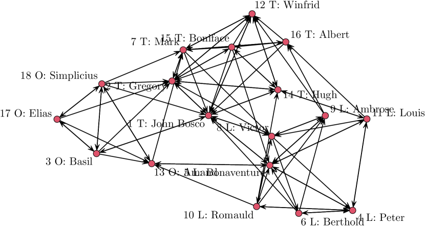
Figure 1: The monks dataset, with edges indicating directed liking relationships at any of three time points and nodes numbered from 1 to 18 and with group membership as assigned by Sampson indicated by L for Loyalists, O for Outcasts, and T for Young Turks.

As an example of the F operator, the code below uses four different methods to summarize the number of ties between pairs of nodes in the Turks group in the samplike dataset:

data(sampson)

summary(samplike ~ nodematch("group", diff=TRUE, levels="Turks")

                 + F(~nodematch("group"), ~nodefactor("group", levels="Turks"))

                 + F(~edges, ~nodefactor("group", levels="Turks") == 2)

                 + F(~edges, ~!nodefactor(~group!="Turks")))

##                                 nodematch.group.Turks
##                                                    30
## F(nodefactor("group",levels="Turks"))~nodematch.group
##                                                    30
##        F(nodefactor("group",levels="Turks")==2)~edges
##                                                    30
##                 F(!nodefactor(~group!="Turks"))~edges
##                                                    30

Here, the third method works because this particular $f_{i,j}(y_{i,j})$ counts how many of the two nodes $i$ and $j$ are Turks, and so equals 2 if and only if both are; and the fourth method works because the new $f_{i,j}(y_{i,j})$ is 0 only if neither $i$ nor $j$ is a non-Turks node.

It is also possible to filter on a quantitative variable. For instance, an alternative way to count the number of edges in faux.mesa.high that match on "Grade" is to report total edges after filtering by node pairs whose absolute difference on the "Grade" variable is less than 1:

cbind(summary(faux.mesa.high ~ nodematch("Grade")),

      summary(faux.mesa.high ~ F(~edges, ~absdiff("Grade") < 1)))

##                 [,1] [,2]
## nodematch.Grade  163  163

While filter must be dyad-independent, formula can have dyad-dependent terms as well. For instance, we may count the transitive triples—i.e., triples $(i,j,k)$ where $y_{i,j}=y_{j,k}=y_{i,k}=1$—in the samplike network, then perform the same count on the subnetwork consisting only of those edges connecting two monks not in attendance in the minor seminary of Cloisterville before coming to the monastery:

summary(samplike ~ ttriple + F(~ttriple, ~nodefactor("cloisterville") == 0))

##                                   ttriple F(nodefactor("cloisterville")==0)~ttriple
##                                       154                                        12

4.1.2 Treating directed networks as undirected

The operator Symmetrize(formula, rule) evaluates the terms in formula on an undirected network constructed by symmetrizing the underlying directed network according to rule. The possible values of rule, which match the terminology of the symmetrize function of the sna package, are (a) “weak”, (b) “strong”, (c) “upper”, and (d) “lower”; for any $i<j$, these four values result in an undirected tie between $i$ and $j$ if and only if (a) either $y_{i,j}$ or $y_{j,i}$ equals 1, (b) both $y_{i,j}$ and $y_{j,i}$ equal 1, (c) $y_{i,j}=1$, and (d) $y_{j,i}=1$. For example,

summary(samplike ~ Symmetrize(~edges, "strong") + mutual + Symmetrize(~edges, "weak") + edges)

## Symmetrize(strong)~edges                   mutual   Symmetrize(weak)~edges
##                       28                       28                       60
##                    edges
##                       88

will compute the number of node pairs $i<j$ with reciprocated edges, equivalent to mutuality, i.e., $y_{i,j}=y_{j,i}=1$, along with the number of node pairs in which at least one edge is present; summing these values yields the total number of directed edges.

4.1.3 Extracting subgraphs

The operator S(formula, attrs) evaluates the terms in formula on an induced subgraph constructed from vertices identified by attrs. The attrs argument either takes a value as explained in Section 3.2 for the nodes= argument or, to obtain a bipartite network, a two-sided formula with the left-hand side specifying the tails and the right-hand side specifying the heads. For instance, suppose that we wish to model the density and mutuality dynamics within the group “Young Turks” as different from those of the rest of the network:

coef(summary(ergm(samplike~edges + mutual + S(~edges + mutual, ~(group == "Turks")),

                  control = snctrl(seed = 123))))

##                             Estimate Std. Error MCMC %   z value     Pr(>|z|)
## edges                      -2.007074  0.2377493      0 -8.441979 3.120095e-17
## mutual                      2.351613  0.4996500      0  4.706519 2.519819e-06
## S((group=="Turks"))~edges   2.812378  0.8650057      0  3.251282 1.148857e-03
## S((group=="Turks"))~mutual -2.165222  1.1965294      0 -1.809585 7.036009e-02

Thus, the density within the group is statistically significantly higher, whereas the reciprocation within the group is lower, though not statistically significantly at the 5% level.

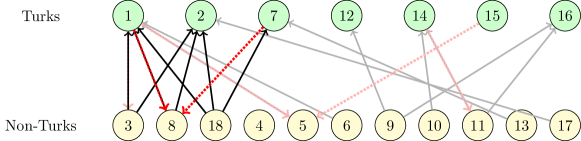
Figure 2: A bipartite induced subgraph between Turks (green) and Non-Turks (yellow). Edges involved in at least one undirected 4-cycle are emphasized. When directed edges from Non-Turks to Turks (black) are viewed as bipartite (undirected) edges, we obtain 4-cycles (3, 1, 18, 2), (3, 1, 8, 2), and (8, 1, 18, 2). When directed edges from Turks to Non-Turks (dotted red) are also included, we obtain the additional 4-cycles (8, 1, 18, 7) and (8, 2, 18, 7).

As another example, illustrated in Figure 2, consider the directed edges from non-Young Turks to Young Turks. Creating the induced subgraph from these edges results in a bipartite network—which is always taken to be undirected even though the edges were originally directed—we may count the number of four-cycles:

summary(samplike ~ S(~cycle(4), (group != "Turks") ~ (group == "Turks")))

## S((group!="Turks"),(group=="Turks"))~cycle4
##                                           3

On the other hand, if we treat the original network as undirected using Symmetrize before creating the induced bipartite subgraph, we see additional four-cycles. This example also illustrates that term operators may be nested arbitrarily:

summary(samplike ~ Symmetrize(~S(~cycle(4), (group != "Turks") ~ (group == "Turks")), "weak"))

## Symmetrize(weak)~S((group!="Turks"),(group=="Turks"))~cycle4
##                                                            5

Finally, we illustrate a common use case in which Symmetrize is used to analyze mutuality in a directed network as a function of a predictor. The faux.dixon.high dataset is a directed friendship network of seventh through twelfth graders. Suppose we wish to check how strongly the tendency toward mutuality in friendships is affected by students’ closeness in grade level.

data(faux.dixon.high)

FDHfit <- ergm(faux.dixon.high ~ edges + mutual + absdiff("grade")

               + Symmetrize(~absdiff("grade"), "strong"), control=snctrl(seed=321))

coef(summary(FDHfit))

##                                    Estimate Std. Error MCMC %    z value      Pr(>|z|)
## edges                            -3.2492290 0.04728446      0 -68.716639  0.000000e+00
## mutual                            3.2447618 0.11742536      0  27.632549 4.523720e-168
## absdiff.grade                    -0.9139858 0.04289319      0 -21.308413 9.485629e-101
## Symmetrize(strong)~absdiff.grade -0.4130642 0.17653795      0  -2.339804  1.929386e-02

After correcting for the overall network density, the propensity for friendships to be reciprocated, and the predictive effect of grade difference on friendship formation, the difference in grade level has a statistically significant negative effect on the tendency to form mutual friendships ($p$-value = 0.019).

4.2 Interaction effects

For binary ERGMs, interactions between dyad-independent ergm terms can be specified in a manner similar to lm and glm via the : and * operators. (See Section 4.1 for a definition of dyad-independent.)

Let us first consider the colon (:) operator. Generally, if term A creates $p_{\texttt{A}}$ statistics and term B creates $p_{\texttt{B}}$ statistics, then A:B will create $p_{\texttt{A}}\times p_{\texttt{B}}$ new statistics. If A and B are dyad-independent terms, expressed for $a=1,\dotsc,p_{\texttt{A}}$ and $b=1,\dotsc,p_{\texttt{B}}$ as

$$g_{\texttt{A}}(\mathbf{y})=\sum_{{{(i,j)}\in\mathbb{Y}}}x^{\texttt{A}}_{i,j}y_{i,j}\text{\ and\ }g_{\texttt{B}}(\mathbf{y})=\sum_{{{(i,j)}\in\mathbb{Y}}}x^{\texttt{B}}_{i,j}y_{i,j}$$

for appropriate covariate matrices $X^{\texttt{A}}$ and $X^{\texttt{B}}$, then the corresponding interaction term is

$$g_{\texttt{A:B}}(\mathbf{y})=\sum_{{{(i,j)}\in\mathbb{Y}}}x^{\texttt{A}}_{i,j}x^{\texttt{B}}_{i,j}y_{i,j}.$$ (3)

As an example, consider the Grade and Sex effects, expressed as model terms via nodefactor, in the faux.mesa.high dataset:

summary(faux.mesa.high ~ nodefactor("Grade", levels = TRUE):nodefactor("Sex"))

##  nodefactor.Grade.7:nodefactor.Sex.M  nodefactor.Grade.8:nodefactor.Sex.M
##                                   70                                   99
##  nodefactor.Grade.9:nodefactor.Sex.M nodefactor.Grade.10:nodefactor.Sex.M
##                                   63                                   46
## nodefactor.Grade.11:nodefactor.Sex.M nodefactor.Grade.12:nodefactor.Sex.M
##                                   38                                   26

In the call above, we deliberately include all Grade-factor levels via levels=TRUE, whereas we employ the default behavior of nodefactor for the Sex factor, which leaves out one level. Thus, the 6-level Grade factor and the 2-level Sex factor, with one level of the latter omitted, produce $6\times 1$ interaction terms in this example.

The * operator, by contrast, produces all interactions in addition to the main effects or statistics. Therefore, in the scenario described above, A*B will add $p_{\texttt{A}}+p_{\texttt{B}}+p_{\texttt{A}}\times p_{\texttt{B}}$ statistics to the model. Below, we use the default behavior of nodefactor on both the 6-level Grade factor and the 2-level Sex factor, together with an additional edges term, to produce a model with $1+5+1+5\times 1$ terms:

m <- ergm(faux.mesa.high ~ edges + nodefactor("Grade") * nodefactor("Sex"))

print(summary(m), digits = 3)

## Call:
## ergm(formula = faux.mesa.high ~ edges + nodefactor("Grade") *
##     nodefactor("Sex"))
##
## Maximum Likelihood Results:
##
##                                      Estimate Std. Error MCMC % z value Pr(>|z|)
## edges                                  -3.028      0.173      0  -17.53  < 1e-04 ***
## nodefactor.Grade.8                     -1.424      0.263      0   -5.41  < 1e-04 ***
## nodefactor.Grade.9                     -1.166      0.229      0   -5.10  < 1e-04 ***
## nodefactor.Grade.10                    -1.633      0.357      0   -4.58  < 1e-04 ***
## nodefactor.Grade.11                    -0.328      0.237      0   -1.38  0.16714
## nodefactor.Grade.12                    -0.794      0.324      0   -2.45  0.01429 *
## nodefactor.Sex.M                       -1.764      0.240      0   -7.36  < 1e-04 ***
## nodefactor.Grade.8:nodefactor.Sex.M     1.386      0.202      0    6.86  < 1e-04 ***
## nodefactor.Grade.9:nodefactor.Sex.M     1.012      0.211      0    4.79  < 1e-04 ***
## nodefactor.Grade.10:nodefactor.Sex.M    1.347      0.264      0    5.11  < 1e-04 ***
## nodefactor.Grade.11:nodefactor.Sex.M    0.419      0.240      0    1.75  0.08074 .
## nodefactor.Grade.12:nodefactor.Sex.M    1.059      0.290      0    3.65  0.00026 ***
## ---
## Signif. codes:  0 ’***’ 0.001 ’**’ 0.01 ’*’ 0.05 ’.’ 0.1 ’ ’ 1
##
##      Null Deviance: 28987  on 20910  degrees of freedom
##  Residual Deviance:  2189  on 20898  degrees of freedom
##
## AIC: 2213  BIC: 2308  (Smaller is better. MC Std. Err. = 0)

Equation (3) implies that the change statistic corresponding to dyad ${(i,j)}$ is given by $x^{\texttt{A}}_{i,j}x^{\texttt{B}}_{i,j}$; that is, the change statistic for the interaction is the product of the change statistics. One may define interaction change statistics for arbitrary pairs of terms similarly—that is, by taking the interaction change statistic as the product of the corresponding change statistics—though in the case of dyad-dependent terms it is unclear that a change statistic obtained as the product of change statistics corresponds to any ERGM sufficient statistic in the sense of Equation (1). Therefore, attempting to create interactions involving dyad-dependent terms will create an error by default in ergm. If one wishes to create such interactions anyway, the default behavior may be changed using the interact.dependent term option as described in Section 8.6.2. Interactions involving curved ERGM terms are not supported in ergm 4.

Since interaction terms are defined by multiplying change statistics dyadwise and then (for dyad-independent terms) summing over all dyads, interactions of terms are not the same as products of those terms. For instance, given a nodal covariate "a", the interaction of nodecov("a") with itself is different than the effect of the square of the covariate, as we observe in the case of the wealth covariate of the (undirected) Florentine marriage dataset:

data(florentine)

summary(flomarriage ~ nodecov("wealth"):nodecov("wealth") + nodecov(~wealth^2))

## nodecov.wealth:nodecov.wealth              nodecov.wealth^2
##                        284058                        187814

4.3 Reparametrizing the model

The term operator Sum(formulas, label) allows arbitrary linear combinations of existing statistics to be added to the model. Suppose $\mathbf{g}_{1}(\mathbf{y}),\dotsc,\mathbf{g}_{K}(\mathbf{y})$ is a set of $K$ vector-valued network statistics, each corresponding to one or more ergm terms and of arbitrary dimension. Also suppose that $A_{1},\dotsc,A_{K}$ is a set of known constant matrices all having the same number of rows such that each matrix multiplication $A_{k}\mathbf{g}_{k}(\mathbf{y})$ is well-defined. Then it is now possible to define the statistic

$$\mathbf{g}_{\text{Sum}}(\mathbf{y})=\sum_{k=1}^{K}A_{k}\mathbf{g}_{k}(\mathbf{y}).$$

The first argument to Sum is a formula or a list of $K$ formulas, each representing a vector statistic. If a formula has a left-hand side, the left-hand side will be used to define the corresponding $A_{k}$ matrix: If it is a scalar or a vector, $A_{k}$ will be a diagonal matrix thus multiplying each element by its corresponding element; and if it is a matrix, $A_{k}$ will be used directly. When no left-hand side is given, $A_{k}$ is defined as 1. To simplify this function for some common cases, if the left-hand side is "sum" or "mean", the sum (or mean) of the statistics in the formula is calculated.

As an example, consider a vector of statistics consisting of the numbers of friendship ties received by each subgroup of Sampson’s monks:

summary(samplike ~ nodeifactor("group", levels = TRUE))

##    nodeifactor.group.Loyal nodeifactor.group.Outcasts    nodeifactor.group.Turks
##                         29                         13                         46

We may create a single statistic equal to the friendship ties received by both groups of non-Outcasts by adding the first and third components of the nodefactor vector, either by left-multiplying by $\begin{bmatrix}1&0&1\end{bmatrix}$ or by deselecting the second component at the nodeifactor level and summing the remaining two:

summary(samplike ~ Sum(cbind(1, 0, 1) ~ nodeifactor("group", levels = TRUE), "nf.L_T") +

                    Sum("sum" ~ nodeifactor("group", levels = -2), "nf.L_T"))

## Sum~nf.L_T Sum~nf.L_T
##         75         75

Whereas the Sum operator operates on network statistics, Parametrize(formula, params, map, gradient=NULL, minpar=-Inf, maxpar=+Inf, cov=NULL) operates on the parameters. The formula argument specifies a vector statistic $\mathbf{g}_{k}(\mathbf{y})$ involving one or more terms and, if curved terms are specified, a mapping $\bm{\eta}_{k}({\bm{\theta}})$. The remaining arguments follow the curved ERGM template: The function map must take arguments x, n, and ... and map the parameter vector (whose length and names are specified by the params argument) into the domain of $\bm{\eta}_{k}$, transforming an ERGM term $\bm{\eta}_{k}({\bm{\theta}}_{k})^{\top}\mathbf{g}_{k}(\mathbf{y})$ to $\bm{\eta}_{k}(\bm{\eta}_{\star}({\bm{\theta}}_{k}))^{\top}\mathbf{g}_{k}(\mathbf{y})$, where $\bm{\eta}_{\star}$ is the function specified by map. The function gradient must take the same arguments as map and return the gradient matrix, minpar and maxpar specify the box constraints of the domain of map, and cov provides an optional argument to map. If formula is not curved, $\bm{\eta}_{k}({\bm{\theta}})$ is simply the identity function.

To simplify this function for some common special cases, if map="rep", the parameter vector will simply be replicated to make it as long as required by $\bm{\eta}_{k}({\bm{\theta}})$, and the gradient will be evaluated automatically. Similarly, if the user is certain that map is linear or affine, the gradient will be calculated automatically if gradient="linear" is specified.

To illustrate this, consider a simple model with the baseline edge effect and a single attractiveness effect for monks who are not Outcasts. Following are four different ways to specify this model:

# Calculated nodal covariate:

f1 <- samplike ~ edges + nodeifactor(~group != "Outcasts")

summary(f1)

##                              edges nodeifactor.group!="Outcasts".TRUE
##                                 88                                 75

# Transform the statistic:

f2 <- samplike ~ edges +

                 Sum(cbind(1,0,1) ~ nodeifactor("group",levels=TRUE), "nf.L_T")

summary(f2)

##      edges Sum~nf.L_T
##         88         75

# Transform the parameters:

f3 <- samplike ~ edges + Parametrize(~nodeifactor("group", levels=TRUE), "nf.L_T",

                               function(x,n,...) c(x,0,x), gradient="linear")

summary(f3)

##                      edges    nodeifactor.group.Loyal nodeifactor.group.Outcasts
##                         88                         29                         13
##    nodeifactor.group.Turks
##                         46

# Select groups, replicate parameter:

f4 <- samplike ~ edges + Parametrize(~nodeifactor("group", levels=-2), "nf.L_T", "rep")

summary(f4)

##                   edges nodeifactor.group.Loyal nodeifactor.group.Turks
##                      88                      29                      46

We may now verify that all four fitted models return the same parameter estimates:

cbind(coef(ergm(f1)), coef(ergm(f2)), coef(ergm(f3)), coef(ergm(f4)))

##                                          [,1]       [,2]       [,3]       [,4]
## edges                              -1.4423838 -1.4423838 -1.4423838 -1.4423838
## nodeifactor.group!="Outcasts".TRUE  0.6661217  0.6661217  0.6661217  0.6661217

Whereas the Sum operator calculates linear combinations of network statistics, the Prod operator calculates the products of their powers. As of this writing, it is implemented for positive statistics only, by first applying the Log operator (which returns the natural logarithm, log in R, of the statistics passed to it), then the Sum operator, and finally the Exp operator (which returns the exponential function, exp in R). As a simple illustration, we may verify that the Sum and Prod operators do in fact produce network statistics as expected if we simply use each with a list of formulas having no left hand side:

summary(faux.dixon.high ~ edges + mutual + Sum(list(~edges, ~mutual), "EdgesAndMutual")

        + Prod(list(~edges, ~mutual), "EdgesAndMutual"))

##                  edges                 mutual     Sum~EdgesAndMutual Exp~Sum~EdgesAndMutual
##                   1197                    219                   1416                 262143

5 Sample space constraints

In Section 1, we saw that the sample space $\mathcal{Y}$ is a subset of the power set $2^{\mathbb{Y}}$, where $\mathbb{Y}$ in itself a subset of all potential relationships. Many applications in fact take $\mathbb{Y}$ to be the set of all relationships and $\mathcal{Y}=2^{\mathbb{Y}}$, but it is sometimes desirable to restrict the sample space by placing constraints on which relationships $(i,j)$ are allowed in $\mathbb{Y}$ and further which networks $\mathbf{y}\in 2^{\mathbb{Y}}$ are allowed in $\mathcal{Y}$. As a simple example, a bipartite network allows only edges connecting nodes from one subset, or mode, to nodes from its complement. This particular constraint is so commonly used that it is hard-coded into network and ergm. As another example, consider the inverse of a bipartite setting, in which edges are only allowed within subsets of the node set, a situation often called a block-diagonal constraint. As still another, some applications impose a cap on the degree of any node, which constrains the sample space to include only those networks in which every node has a permitted degree.

In all of the cases above, correct statistical inference for ERGMs depends on correctly incorporating constraints into the fitting process. They are specified using the constraints argument, a one-sided formula whose terms specify the constraints on the sample space. For example, constraints = ~edges specifies $\mathcal{Y}^{\text{{edges}}}=\{\mathbf{y}^{\prime}\in\mathcal{Y}:\lvert\mathbf{y}^{\prime}\rvert=\lvert\mathbf{y}\rvert\}$, where $\mathbf{y}$ is the observed network, specified on the left-hand side. Some constraints, such as fixedas(y1,y0) focus on constraining $\mathbb{Y}$—in this case, as $\mathbb{Y}^{\text{{fixedas(y1,y0)}}}=\{{{(i,j)}\in\mathbb{Y}}:{(i,j)}\in\mathbf{y}^{1}\land{(i,j)}\notin\mathbf{y}^{0}\}$—with $\mathcal{Y}\equiv 2^{\mathbb{Y}}$.

Multiple constraints can be specified on a formula, separated by + to impose a new constraint in additional to prior or (in some instances) - to relax preceding constraints. Earlier versions of the ergm package implemented a number of constraints, as described for example in Section 3 of Morris et al. (2008). Since that time, many additional types of constraints and methods for imposing them have been added, some of which we describe in this section. A full list of currently implemented constraints is obtained via ? ergmConstraint, and a specific constraint [name] can be looked up with help("[name]-ergmConstraint") or ergmConstraint?[name].

5.1 Arbitrary combinations of dyad-independent constraints

In general, every combination of constraints requires a somewhat different Metropolis–Hastings proposal algorithm for efficient sampling, and so it may be impractical support every possible combination of constraints. Dyad-independent constraints, which affect $\mathcal{Y}$ only through $\mathbb{Y}$, and do not induce stochastic dependencies among the dyad states, are an exception. These include constraining specific dyads (such as the above-mentioned observed and fixedas constraints), dyads incident on specific actors (such as the egocentric constraint), and block-diagonal structure; and any combination of dyad-independent constraints is a dyad-independent constraint. For some such combinations, ergm and other packages provide optimized implementations. For the rest, ergm falls back to a general but efficient implementation that uses run-length encoding tools provided by package rle (Krivitsky, 2020) to efficiently store sets of non-constrained dyads and rejection sampling to efficiently select a dyad for the proposal.

Here, we illustrate some of ergm’s capabilities using a dataset due to Coleman (1964) that is small enough that computational inefficiency will not present problems. These data are self-reported friendship ties among 73 boys measured at two time points during the 1957–1958 academic year and they are included as a $2\times 73\times 73$ array and documented in the sna package. We use the Coleman data to create a network object with $2\times 73$ nodes:

library(sna)

data(coleman)

cole <- matrix(0, 2 * 73, 2 * 73)

# Upper left and lower right blocks:

cole[1:73, 1:73] <- coleman[1, , ]

cole[73 + (1:73), 73 + (1:73)] <- coleman[2, , ]

# Upper right and lower left blocks:

diag(cole[1:73, 73 + (1:73)]) <- diag(cole[73 + (1:73), 1:73]) <- 1

ncole <- network(cole)

ncole %v% "Semester" <- rep(c("Fall", "Spring"), each = 73)

ncole

##  Network attributes:
##   vertices = 146
##   directed = TRUE
##   hyper = FALSE
##   loops = FALSE
##   multiple = FALSE
##   bipartite = FALSE
##   total edges= 652
##     missing edges= 0
##     non-missing edges= 652
##
##  Vertex attribute names:
##     Semester vertex.names
##
## No edge attributes

By construction, the ncole network includes the Fall 1957 semester data and the Spring 1958 data as the upper left $73\times 73$ and lower right $73\times 73$ blocks, respectively. In addition, the upper right and lower left blocks indicate which nodes are the same person; that is, $y_{i,j}=1$ whenever $i$ and $j$ are the same boy measured at two different times. This latter information is redundant because the ordering of the 73 boys is the same in both fall and spring, yet we include it to illustrate some techniques using entries that are not on the main block diagonal and because in principle it might not always be the case that the same individuals are observed at both time points.

5.2 Constraints via the Dyads operator

The Dyads(fix=NULL, vary=NULL) operator takes one or two ergm formulas that may contain only dyad-independent terms. For the terms in the fix= formula, dyads that affect the network statistic (i.e., have nonzero change statistic) for any the terms will be fixed at their current values. For the terms in the vary= formula, only those that change at least one of the terms will be allowed to vary, and all others will be fixed. If both formulas are given, the dyads that vary either for one or for the other will be allowed to vary. A formula passed without an argument name will default to fix=, for consistency with other constraints’ semantics.

The key to our treatment of the ncole network using the Dyads operator is the Semester vertex attribute:

table(ncole %v% "Semester")

##
##   Fall Spring
##     73     73

In particular, the nodematch("Semester") term has a change statistic equal to one for exactly those dyads representing boys measured during the same semester, and this change statistic is zero otherwise. Therefore, in our 146-node directed network there are $146\times 145$, or $21{,}170$, total dyads, of which $2\times 73\times 72$, or $10{,}512$, have nonzero change statistics for nodematch("Semester"). We can easily see exactly how many total edges there are and how many of these are in the upper left or lower right blocks:

summary(ncole ~ edges + nodematch("Semester"))

##              edges nodematch.Semester
##                652                506

We can now calculate directly the log-odds, or logit, for both the block diagonal and the off-block diagonal subnetworks, then verify that the Dyads operator can accomplish these same calculations using a constrained ERGM. First, we fix dyads with nonzero change statistics, which corresponds to the block off-diagonal entries:

logit <- function(p) log(p/(1-p))

cbind(logit((652 - 506) / (21170 - 10512)),

      coef(ergm(ncole ~ edges, constraints = ~Dyads(fix = ~nodematch("Semester")))))

##            [,1]      [,2]
## edges -4.276666 -4.276666

Next, we allow dyads with nonzero change statistics to vary, which corresponds to the block diagonal entries:

cbind(logit(506 / 10512),

      coef(ergm(ncole ~ edges, constraints = ~Dyads(vary = ~nodematch("Semester")))))

##            [,1]      [,2]
## edges -2.984404 -2.984404

If we remove the constraints entirely, ncole has 652 edges out of a possible $21{,}170$:

cbind(logit(652/21170), coef(ergm(ncole ~ edges)))

##            [,1]      [,2]
## edges -3.449013 -3.449013

A significant limitation of this specific constraint is that its initialization requires testing every possible dyad and therefore takes up time and memory in proportion to the square of the number of nodes.

5.3 Constraints via blocks

The blocks operator constrains changes to any dyads that involve certain pairs of categories defined by a particular nodal covariate. We may reproduce the examples of Section 5.2 using blocks. First, consider the full complement of statistics produced by the nodemix model term:

summary(ncole ~ nodemix("Semester", levels = TRUE, levels2 = TRUE))

##     mix.Semester.Fall.Fall   mix.Semester.Spring.Fall   mix.Semester.Fall.Spring
##                        243                         73                         73
## mix.Semester.Spring.Spring
##                        263

The levels = TRUE argument ensures that nodemix considers every value of "group" in constructing a mixing matrix of possible dyad combinations. The levels2 = TRUE argument ensures that, from the full complement of such possible combinations, every one is included as a statistic. By default, levels = TRUE whereas levels2 = -1, since we frequently want to exclude at least one possible mixing combination to avoid collinearity in a model that also includes the edges term.

We may now use levels2 in conjunction with blocks to select exactly which of the nodemix combinations should be constrained as fixed to reproduce the examples of Section 5.2. First, we fix all dyads where the group values do not match:

coef(ergm(ncole ~ edges, constraints = ~blocks("Semester", levels2 = c(1, 4))))

##     edges
## -4.276666

Second, we fix the dyads where group values do match:

coef(ergm(ncole ~ edges, constraints = ~blocks("Semester", levels2 = c(2, 3))))

##     edges
## -2.984404

Additional examples using levels2, among other nodal attribute features, are contained in the nodal_attributes vignette within the ergm package.

5.4 Additional constraints

Multiple different constraints on the sample space of possible networks, as defined by the values of certain network statistics, may be implemented beyond those discussed already in this section. The bd constraint, for instance, may be used to enforce a maximum allowable degree for any node, via the maxout argument. A comprehensive list of available constraints is available via ? ergmConstraint. The handling of various constraints by MCMC proposals in the ergm package is addressed in Krivitsky et al. (2022).

6 Modeling Networks with Valued Edges

Starting with version 3.1, the ergm package can handle some types of networks whose ties are not merely binary, indicating presence or absence, but may have nonzero values other than unity. For example, the value of a tie might represent a count, such as the number of times a particular relationship has occurred; or it might represent an ordinal variable, if node $i$ ranks a subset of its neighbors. Valued ties can increase complexity relative to binary ties in, for example, specifying the model and ensuring that the chosen statistics are meaningful for the types of edge values being modeled. Whether the scale of measurement of tie values is ordinal, interval, or ratio, it becomes necessary to specify the distribution of these values and to create functions to aggregate these values into ERGM statistics.

In the ergm(), simulate(), and summary() functions, the valued mode is typically activated by passing a response= argument, giving the name of the edge attribute containing the value of the response. Non-edges are assumed to have value 0. The argument may also be a formula whose right-hand side is an expression in terms of the edge attributes that evaluates to the response value and whose left-hand side, if present, gives the name to be used. If it evaluates to a logical (TRUE/FALSE) value (e.g., response=threeContacts~(contacts>=3)), a binary ERGM is used.

6.1 Reference specification

Krivitsky (2012) pointed out that sufficient statistics alone do not suffice to specify an ERGM on a network whose relations are valued. Consider a simple ERGM of the form

$$\operatorname{Pr}(\mathbf{Y}=\mathbf{y};\theta)\propto h(\mathbf{y})\exp\left(\theta\sum_{{{(i,j)}\in\mathbb{Y}}}y_{i,j}\right),$$ (4)

where $y_{i,j}\in\{0,1,\dotsc\}$ is an unbounded count. If $h(\mathbf{y})$ is any constant, then $Y\!_{i,j}{\stackrel{{\scriptstyle\mathrm{i.i.d.}}}{{\sim}}}\operatorname{Geometric}[p=1-\exp\left(\theta\right)]$. On the other hand, if $h(\mathbf{y})=1/\prod_{{{(i,j)}\in\mathbb{Y}}}y_{i,j}!$, then $Y\!_{i,j}{\stackrel{{\scriptstyle\mathrm{i.i.d.}}}{{\sim}}}\operatorname{Poisson}[\mu=\exp\left(\theta_{k}\right)]$. For this reason, Krivitsky (2012) called a distribution with $h(\mathbf{y})=1$ and a sample space of nonnegative integers a Geometric-reference ERGM and one with $h(\mathbf{y})=1/\prod_{{{(i,j)}\in\mathbb{Y}}}y_{i,j}!$ a Poisson-reference ERGM.

For ergm(), simulate(), and other functions, reference distributions are specified with a reference= argument, which is a one-sided formula with one term. The ergm package allows Unif(a,b) and DiscUnif(a,b) references, specifying $h(\mathbf{y})=1$, the former on a dyad space $y_{i,j}\in[a,b]$, the latter on $y_{i,j}\in\{a,a+1,\dotsc,b\}$. A companion package, ergm.count, allows the additional references Poisson and Geometric, described above, as well as Binomial(trials) for $h(\mathbf{y})=\prod_{{{(i,j)}\in\mathbb{Y}}}\binom{n_{\text{trials}}}{y_{i,j}}$ in the case $y_{i,j}\in\{0,\dotsc,n_{\text{trials}}\}$. For rank-order relational data, a CompleteOrder reference distribution is implemented in the ergm.rank package for situations where rankings are compete. Where ties are permitted, DiscUnif() can be used as a reference. See Krivitsky & Butts (2019) for further details on both the ergm.count and ergm.rank packages, and their vignettes.

Reference distributions are explained in more detail in Section 3 of Krivitsky & Butts (2019). This reference also illustrates how the network package may be used to visualize some kinds of valued networks (Section 2) and even how the latentnet package can handle latent-space models with valued ties (Section 4). Online help on the reference distributions that are implemented by all packages currently loaded in an R session can be obtained by typing help("ergm-references").

6.2 Dyad-Independent statistics

As in Section 4.1, a component of the vector $\mathbf{g}(\mathbf{y})$ is called a dyad-independent statistic if, when one builds an ERGM using it as the only model statistic, the joint distribution (1) of the network factors into the product of its marginal dyad distributions. That is, the univariate version of equation (1) may be written

$$\operatorname{Pr}(\mathbf{Y}=\mathbf{y};\theta)=\prod_{{{(i,j)}\in\mathbb{Y}}}\operatorname{Pr}(Y\!_{i,j}=y_{i,j})=\frac{h(\mathbf{y})}{\kappa_{h,\eta,g}(\theta,\mathcal{Y})}\prod_{{{(i,j)}\in\mathbb{Y}}}\exp\{\eta(\theta)g_{{i,j}}(\mathbf{y})\}$$ (5)

for ${\mathbf{y}\in\mathcal{Y}}$ and for some appropriately chosen $g_{{i,j}}(\mathbf{y})$. Equation (4) shows that the sum of the values $y_{i,j}$, which implies $g_{{i,j}}(\mathbf{y})=y_{i,j}$, is one such example. Another example is the sum of the nonzero indicators that arises if we define $g_{{i,j}}(\mathbf{y})=\mathbb{I}\{y_{i,j}>0\}$. Each of these basic dyad-independent statistics is implemented in ergm:

sum(pow=1) Sum of edge values

This is simply the summation of edge values. For most valued ERGMs, this is the natural intercept term. In particular, for reference distributions such as Poisson and Binomial, using this term produces intercept effects of Poisson log-linear and binomial logistic regressions, respectively. Optionally, the dyad values can be raised to a power before being summed.

nonzero Number of nonzero edge values

This term counts nonzero edge values. It can be used to model zero-inflation that is common in networks: It is often the case that a network is sparse but has edges with relatively high weights when they are present.

Binary ERGM statistics cannot be used directly for valued networks nor vice versa, but most dyad-independent binary ERGM statistics have been generalized by imposing a covariate on one of the two above forms. They have the same arguments as their binary ERGM counterparts, with an additional argument: form, which has two possible values: "sum" (the default) and "nonzero". The former creates a statistic of the form $\sum_{{{(i,j)}\in\mathbb{Y}}}x_{i,j}y_{i,j}$, where $y_{i,j}$ is the value of dyad $(i,j)$ and $x_{i,j}$ is the term’s covariate associated with it. The latter computes a sum of indicator variables, one for each dyad, indicating whether the corresponding edge has a nonzero value. When form="sum" is used, typically a GLM-like effect results, whereas form="nonzero" can be used to model sparsity effects. (Krivitsky, 2012) Krivitsky & Butts (2019) gives an example of the form= argument with the nodematch term.

Other terms that control a dyad’s distribution are atleast(threshold = 0), atmost(threshold = 0), equalto(value = 0, tolerance = 0), greaterthan(threshold = 0), ininterval(lower = -Inf, upper = +Inf, open = c(TRUE, TRUE)), and smallerthan(threshold = 0). Each of these terms counts the dyad values that satisfy the criterion identified by its name.

6.3 Mutuality

The binary mutuality term in ergm counts the number of pairs of mutual ties. Its valued counterpart is mutuality(form), which permits the following values of form. For each of these, a higher coefficient will tend to increase the similarity of reciprocating dyad values.

"product" Sum of products of reciprocating edge values

This is the most direct generalization. However, for a Poisson-reference ERGM in particular, a positive coefficient on this term produces an infinite normalizing constant and therefore lies outside the parameter space.

"geometric" Sum of geometric mean of reciprocating edge values

This form solves the product form’s problem by taking a square root of the product. It can be viewed as the uncentered covariance of variance-stabilized counts.

"min" Minimum of reciprocating edge values

This effect is, perhaps, the easiest to interpret, at the cost of statistical power.

"nabsdiff" Absolute difference of reciprocating edge values

This effect is more symmetrical than min.

We refer the reader to Krivitsky (2012) for a further discussion of the effects.

6.4 Actor heterogeneity

Different actors may have different overall propensities to interact. This has been modeled using random effects, as in the $p_{2}$ model, and using degeneracy-prone terms like $k$-star counts. For valued ERGMs, the following term, also introduced by Krivitsky (2012) and discussed in more detail there, models actor heterogeneity:

nodesqrtcovar(center,transform) Covariance between $y_{i,j}$ incident on same actor

The default transform="sqrt" will take a square root of dyad values before calculating, and the default center=TRUE will center the transformed values around their global mean, gaining stability at the cost of locality.

6.5 Triadic effects

To generalize the notion of triadic closure, ergm implements very flexible transitiveweights(twopath, combine, affect) and similar cyclicalweights statistics. The transitive weight statistic has the general form

$$g_{\text{$\bm{v}$}}(\mathbf{y})=\sum_{{{(i,j)}\in\mathbb{Y}}}v_{\text{affect}}\left(y_{i,j},v_{\text{combine}}\left(v_{\text{2-path}}(\mathbf{y}_{i,k},\mathbf{y}_{k,j})_{k\in N\backslash\{i,j\}}\right)\right),$$

which can be customized by varying three functions:

$v_{\text{2-path}}$

Given $\mathbf{y}_{i,k}$ and $\mathbf{y}_{k,j}$, what is the strength of the two-path they form? The options are "min", to take the minimum of the two-path’s constituent values, and "geomean", to take their geometric mean, gaining statistical power at a greater risk of model instability.

$v_{\text{combine}}$

Given the strengths of the two-paths $\mathbf{y}_{i\to k\to j}$ for all $k\neq i,j$, what is the combined strength of these two-paths between $i$ and $j$? The choices are "max", for the strength of the strongest of the two-paths—analogous to transitiveties or gwesp(0) binary ERGM effects—and "sum", the sum of the path strengths. The latter choice is better able to detect effects but is more subject to degeneracy; it is analogous to triangles.

$v_{\text{affect}}$

Given the combined strength of the two-paths between $i$ and $j$, how should they affect $Y\!_{i,j}$? The choices are "min", the minimum of the combined strength and the focus two-path, and "geomean", again more able to detect effects but more likely to cause degeneracy.

Usage of the transitiveweights and cyclicalweights terms is illustrated in Section 3.1 of Krivitsky & Butts (2019).

6.6 Using binary ERGM terms in valued ERGMs

ergm also allows general binary terms to be passed to valued models. The mechanism that allows this is the term operator B(formula, form), which is further described in the ergm online help under help("B-ergmTerm") or the shorthand ergmTerm?B. Here, formula= is a one-sided formula whose right hand side contains the binary ergm terms to be used. Allowable values of the form argument are form="sum" and form="nonzero", which have the effects described in Section 6.2, with form="sum" only valid for dyad-independent formula= terms; or a one-sided formula may be passed to form=, containing one valued ergm term, with the following properties:

• dyadic independence;

• dyadwise contribution of either 0 or 1;

• dyadwise contribution of 0 for a 0-valued dyad.

That is, it must be expressible as

$$g(y)=\sum_{{{(i,j)}\in\mathbb{Y}}}g_{i,j}(y_{i,j}),$$

where for all $i$, $j$, and $\mathbf{y}$, $g_{i,j}(y_{i,j})\in\{0,1\}$ and $g_{i,j}(0)\equiv 0$. Such terms include nonzero, ininterval(), atleast(), atmost(), greaterthan(), lessthan(), and equalto(). The operator will then construct a binary network $\mathbf{y}^{\text{B}}$ such that $y_{i,j}^{\text{B}}=1$ if and only if $g_{i,j}(y_{i,j})=1$, and evaluate the binary terms in formula= on it.

6.7 Modeling Ordinal Values Using Binary Term Operators

To illustrate the use of binary ergm terms on a valued network as described above, we construct an example that uses the B (for “binary”) operator. The code snippet below gives an example of a valued ergm that uses the DiscUnif, or discrete uniform, reference distribution, which is included in the ergm package itself; that is, there is no need to load the ergm.count or ergm.rank packages to run the following example. The example fits a multinomial logistic regression model that assumes that the edge values independent of one another and take ordinal values that have the same interpretation for each dyad. (In general, rating and ranking data may not allow edge values to be compared across egos (Krivitsky & Butts, 2017); the ergm.rank package contains terms that remain valid in this more complex setting.) Models for independently observed ordinal random variables have a long history in the statistical literature; relevant references specific to network models include Robins et al. (1999) and, in a Bayesian framework, Caimo & Gollini (2020).

First, we build a valued network by pooling the three binary friendship nomination networks due to Sampson (1968), exactly as in Section 2.1 of Krivitsky & Butts (2019).

data(samplk)

# Create a sociomatrix totaling the nominations.

samplk.tot.m <- as.matrix(samplk1) + as.matrix(samplk2) + as.matrix(samplk3)

samplk.tot <- as.network(samplk.tot.m, directed=TRUE, matrix.type="a",

                         ignore.eval=FALSE, names.eval="nominations")

We will use the B operator to construct new statistics consisting of the number of edges with value $k$ or higher, where $k$ is 1, 2, or 3.

summary(samplk.tot ~ B(~edges, ~atleast(1)) + B(~edges, ~atleast(2))

                   + B(~edges, ~atleast(3)), response = "nominations")

## B(atleast(1))~edges B(atleast(2))~edges B(atleast(3))~edges
##                  88                  50                  30

Since there are $18\times 17$, or 306, possible edges, the summary statistics above tell us that the valued network we have constructed has 30 edges with value 3, 20 with value 2, 38 with value 1, and the remaining 218 with value 0. The ERGM with these statistics has independent edges, where the probabilities an edge takes the values 0, 1, 2, or 3 are given by $1/D$, $\exp\{\theta_{1}\}/D$, $\exp\{\theta_{1}+\theta_{2}\}/D$, and $\exp\{\theta_{1}+\theta_{2}+\theta_{3}\}/D$, respectively, where

$$D=1+\exp\{\theta_{1}\}+\exp\{\theta_{1}+\theta_{2}\}+\exp\{\theta_{1}+\theta_{2}+\theta_{3}\}.$$

We may verify that ergm’s stochastic fitting algorithm obtains MLEs very close to the exact values:

mod <- ergm(samplk.tot ~ B(~edges, ~atleast(1)) + B(~edges, ~atleast(2))

          + B(~edges, ~atleast(3)), response = "nominations",

          reference = ~DiscUnif(0,3), control = snctrl(seed = 123))

coef(mod) # Approximate MLEs for theta1, theta2, and theta3

## B(atleast(1))~edges B(atleast(2))~edges B(atleast(3))~edges
##          -1.7342318          -0.6602796           0.4090445

true <- c(EdgeVal0=218, EdgeVal1=38, EdgeVal2=20, EdgeVal3=30)

est <- c(1, exp(cumsum(coef(mod))), use.names=FALSE)

rbind(True_Proportions = true / sum(true), Estimated_Proportions = est / sum(est))

##                        EdgeVal0 EdgeVal1   EdgeVal2   EdgeVal3
## True_Proportions      0.7124183 0.124183 0.06535948 0.09803922
## Estimated_Proportions 0.7117086 0.125642 0.06492009 0.09772932

This example could have used the equalto terms in place of all the atleast terms above. Then, the estimated proportions would have been proportional to 1, $\exp\{\theta_{1}\}$, $\exp\{\theta_{2}\}$, and $\exp\{\theta_{3}\}$ instead of 1, $\exp\{\theta_{1}\}$, $\exp\{\theta_{1}+\theta_{2}\}$, and $\exp\{\theta_{1}+\theta_{2}+\theta_{3}\}$. Such a model does not assume ordinality of the edge values, so it could be used for a multinomial logit model in which the edges take categorical non-ordered values.

7 Estimation in the presence of missing edge data

It is quite common that network data are incomplete in various ways. The ergm package includes the capability to handle missing edge data, whereas other types of missingness such as missing nodal information are not addressed. Handcock & Gile (2010) formulated a framework for modeling networks with missing ties and expressed the log-likelihood as

$$\ell({\bm{\theta}})=\log\operatorname{Pr}(\mathbf{Y}\in\mathcal{Y}(\mathbf{y}^{\text{obs}});{\bm{\theta}})=\log\sum_{{\mathbf{y}^{\prime}\in\mathcal{Y}}(\mathbf{y}^{\text{obs}})}\operatorname{Pr}(\mathbf{Y}=\mathbf{y}^{\prime};{\bm{\theta}}),$$ (6)

where $\mathcal{Y}(\mathbf{y}^{\text{obs}})$ is defined as the set of networks whose partial observation could have produced $\mathbf{y}^{\text{obs}}$: essentially, all of the ways to impute the missing ties in $\mathbf{y}^{\text{obs}}$. (When there are no missing ties in $\mathbf{y}^{\text{obs}}$, $\mathcal{Y}(\mathbf{y}^{\text{obs}})$ contains only $\mathbf{y}^{\text{obs}}$.) They then proposed to maximize this likelihood by taking advantage of the fact that, if

$$\kappa_{\mathcal{Y}^{\prime}}({\bm{\theta}})\stackrel{{\scriptstyle\text{def}}}{{=}}\sum_{\mathbf{y}^{\prime}\in\mathcal{Y}^{\prime}}h(\mathbf{y}^{\prime})\exp\{\bm{\eta}({\bm{\theta}})^{\top}\mathbf{g}(\mathbf{y}^{\prime})\},$$

the log-likelihood can be expressed as $\ell({\bm{\theta}})=\log\kappa_{\mathcal{Y}(\mathbf{y}^{\text{obs}})}({\bm{\theta}})-\log\kappa_{\mathcal{Y}}({\bm{\theta}}),$ resulting in the score equation

$$\bm{\nabla}_{{\bm{\theta}}}\ell(\hat{{\bm{\theta}}})=\bm{\eta}^{\prime}(\hat{{\bm{\theta}}})^{\top}[\operatorname{E}_{\mathcal{Y}(\mathbf{y}^{\text{obs}})}\{\mathbf{g}(\mathbf{Y});\hat{{\bm{\theta}}}\}-\operatorname{E}_{\mathcal{Y}}\{\mathbf{g}(\mathbf{Y});{\hat{{\bm{\theta}}}}\}]=\operatorname{\mathbf{0}},$$

with MCMLE approximation also possible for the first term by fixing a particular ${\bm{\theta}}^{t}$ and drawing a sample from $\operatorname{ERGM}_{\mathcal{Y}(\mathbf{y}^{\text{obs}})}({\bm{\theta}}^{t})$ as explained in Section 3 of Krivitsky et al. (2022).

The ergm package invokes the above approach automatically when a network has missing edge variables. The simplest way to encode a missing edge is to set its value to NA. The network package natively supports missing edge variables coded in this way, and network objects with missingness are thus handled without additional intervention. ergm’s methods for assessing goodness of fit of a model by comparing observed values of certain network statistics to the distribution of their simulated values under the model (Hunter, Goodreau, et al., 2008, p. @HuHa08e) have also been adapted to missing edge data: the (unavailable) observed values of the statistics of interest $t(\mathbf{y})$ are replaced by their conditional expectations $\operatorname{E}_{\mathcal{Y}(\mathbf{y}^{\text{obs}})}\{t(\mathbf{Y});\hat{{\bm{\theta}}}\}$.

Here we fit a simple model with edges, mutuality (reciprocated dyads), transitive ties, and cyclical ties to the Sampson Monks dataset depicted in Figure 1. For the sake of comparison, we first fit the model assuming no missing edge data, which may be quickly verified using the output of the print(samplike) command:

print(samplike)

##  Network attributes:
##   vertices = 18
##   directed = TRUE
##   hyper = FALSE
##   loops = FALSE
##   multiple = FALSE
##   total edges= 88
##     missing edges= 0
##     non-missing edges= 88
##
##  Vertex attribute names:
##     cloisterville group vertex.names
##
##  Edge attribute names:
##     nominations

summary(full.fit <- ergm(samplike ~ edges + mutual + transitiveties + cyclicalties,

                         eval.loglik=TRUE), control = snctrl(seed = 321))

## Call:
## ergm(formula = samplike ~ edges + mutual + transitiveties + cyclicalties,
##     eval.loglik = TRUE)
##
## Monte Carlo Maximum Likelihood Results:
##
##                Estimate Std. Error MCMC % z value Pr(>|z|)
## edges           -1.9436     0.3542      0  -5.488   <1e-04 ***
## mutual           2.5066     0.4551      0   5.507   <1e-04 ***
## transitiveties   0.5499     0.2880      0   1.909   0.0562 .
## cyclicalties    -0.4582     0.2393      0  -1.915   0.0555 .
## ---
## Signif. codes:  0 ’***’ 0.001 ’**’ 0.01 ’*’ 0.05 ’.’ 0.1 ’ ’ 1
##
##      Null Deviance: 424.2  on 306  degrees of freedom
##  Residual Deviance: 329.0  on 302  degrees of freedom
##
## AIC: 337  BIC: 351.9  (Smaller is better. MC Std. Err. = 0.5904)

Now, suppose that Monk #1 (John Bosco) refused to respond during all three waves, rendering his replies missing:

samplike1 <- samplike

samplike1[1, ] <- NA

print(samplike1)

##  Network attributes:
##   vertices = 18
##   directed = TRUE
##   hyper = FALSE
##   loops = FALSE
##   multiple = FALSE
##   total edges= 99
##     missing edges= 17
##     non-missing edges= 82
##
##  Vertex attribute names:
##     cloisterville group vertex.names
##
##  Edge attribute names:
##     nominations

If we pass this modified object to ergm, it will automatically calculate the MLE under the assumption that the monk’s refusal is unrelated to his choice of relations, i.e., that the data are ignorably missing with respect to the specified model:

summary(m1.fit <- ergm(samplike1~edges+mutual+transitiveties+cyclicalties,

                       eval.loglik=TRUE), control = snctrl(seed = 321))

## Call:
## ergm(formula = samplike1 ~ edges + mutual + transitiveties +
##     cyclicalties, eval.loglik = TRUE)
##
## Monte Carlo Maximum Likelihood Results:
##
##                Estimate Std. Error MCMC % z value Pr(>|z|)
## edges           -2.0142     0.3839      0  -5.246   <1e-04 ***
## mutual           2.4206     0.4677      0   5.175   <1e-04 ***
## transitiveties   0.4726     0.4001      0   1.181    0.238
## cyclicalties    -0.3013     0.3455      0  -0.872    0.383
## ---
## Signif. codes:  0 ’***’ 0.001 ’**’ 0.01 ’*’ 0.05 ’.’ 0.1 ’ ’ 1
##
##      Null Deviance: 400.6  on 289  degrees of freedom
##  Residual Deviance: 314.5  on 285  degrees of freedom
##
## AIC: 322.5  BIC: 337.2  (Smaller is better. MC Std. Err. = 0.5524)

The degrees of freedom associated with the missing data fit have decreased because unobserved dyads do not carry information. For details regarding the ignorability assumption for edge variables, see Handcock & Gile (2010).

The estimation approach above can be extended to other types of incomplete network observation. Karwa et al. (2017) applied it to fit arbitrary ERGMs to networks whose dyad values had been stochastically perturbed—ties added and removed at random, with known probabilities—in order to preserve privacy. Another use case is multiple imputation for networks with missing data, in which multiple random versions of the full network are constructed by randomly inserting values for unobserved dyads according to probabilities that are determined based on, say, some type of logistic regression model. These mechanisms may be invoked by passing an obs.constraints formula, specifying how the network of interest was observed. Of particular interest are the following constraints:

observed

restricts the proposal to changing only those dyads that are recorded as missing.

egocentric(attr = NULL, direction = c("both","out","in"))

restricts the proposal to changing only those dyads that would not be observed in an egocentric sample. That is, dyads cannot be modified that are incident on vertices for which attribute specification attr has value TRUE or, if attr is NULL, the vertex attribute "na" has value FALSE. For directed networks, direction=="out" only preserves the out-dyads of those actors, and direction=="in" preserves their in-dyads.

dyadnoise(p01,p10)

Unlike the others, this is a soft constraint to adjust the sampled distribution for dyad-level noise with known perturbation probabilities, which can arise in a variety of contexts (Karwa et al., 2017). It is assumed that the observed LHS network is a noisy observation of some unobserved true network, with p01 giving the dyadwise probability of erroneously observing a tie where the true network had a non-tie and p10 giving the dyadwise probability of erroneously observing a nontie where the true network had a tie. p01 and p10 can be either both be scalars or both be adjacency matrices of the same dimension as that of the LHS network giving these probabilities.

We may use the obs.constraints argument to re-fit the model above:

samplike2 <- samplike

samplike2[1,] <- 0

samplike2 %v% "refused" <- rep(c(TRUE,FALSE),c(1,17))

samplike2 # same as print(samplike2)

##  Network attributes:
##   vertices = 18
##   directed = TRUE
##   hyper = FALSE
##   loops = FALSE
##   multiple = FALSE
##   total edges= 82
##     missing edges= 0
##     non-missing edges= 82
##
##  Vertex attribute names:
##     cloisterville group refused vertex.names
##
##  Edge attribute names:
##     nominations

summary(m2.fit <- ergm(samplike2 ~ edges + mutual + transitiveties + cyclicalties,

                       obs.constraints = ~ egocentric(~!refused, "out"),

                       control = snctrl(seed = 123)))

## Call:
## ergm(formula = samplike2 ~ edges + mutual + transitiveties +
##     cyclicalties, obs.constraints = ~egocentric(~!refused, "out"),
##     control = snctrl(seed = 123))
##
## Monte Carlo Maximum Likelihood Results:
##
##                Estimate Std. Error MCMC % z value Pr(>|z|)
## edges           -2.0090     0.3867      0  -5.196   <1e-04 ***
## mutual           2.3890     0.4764      0   5.015   <1e-04 ***
## transitiveties   0.4401     0.4353      0   1.011    0.312
## cyclicalties    -0.2660     0.3918      0  -0.679    0.497
## ---
## Signif. codes:  0 ’***’ 0.001 ’**’ 0.01 ’*’ 0.05 ’.’ 0.1 ’ ’ 1
##
##      Null Deviance: 400.6  on 289  degrees of freedom
##  Residual Deviance: 313.9  on 285  degrees of freedom
##
## AIC: 321.9  BIC: 336.6  (Smaller is better. MC Std. Err. = 0.4579)

Finally, since the observational process can be viewed as a part of the network dataset, we may specify it using the %ergmlhs% operation, giving a third way to fit the model above:

samplike2 %ergmlhs% "obs.constraints" <- ~egocentric(~!refused, "out")

summary(m3.fit <- ergm(samplike2 ~ edges + mutual + transitiveties + cyclicalties),

        control = snctrl(seed = 231))

## Call:
## ergm(formula = samplike2 ~ edges + mutual + transitiveties +
##     cyclicalties)
##
## Monte Carlo Maximum Likelihood Results:
##
##                Estimate Std. Error MCMC % z value Pr(>|z|)
## edges           -2.0540     0.3964      0  -5.182   <1e-04 ***
## mutual           2.4278     0.4918      0   4.937   <1e-04 ***
## transitiveties   0.5004     0.4377      0   1.143    0.253
## cyclicalties    -0.3118     0.3949      0  -0.789    0.430
## ---
## Signif. codes:  0 ’***’ 0.001 ’**’ 0.01 ’*’ 0.05 ’.’ 0.1 ’ ’ 1
##
##      Null Deviance: 400.6  on 289  degrees of freedom
##  Residual Deviance: 311.8  on 285  degrees of freedom
##
## AIC: 319.8  BIC: 334.4  (Smaller is better. MC Std. Err. = 0.6203)

8 Other enhancements

We close this paper by highlighting a number of miscellaneous enhancements to the ergm package since the Hunter, Handcock, et al. (2008) article.

8.1 Exact calculations for small networks

For small networks, it is possible to obtain full enumeration of all possible network statistic vectors over the entire sample space of possible networks. This enumeration enables exact calculations of such quantities as the log-likelihood function, the MLE, or the normalizing constant. If we consider only binary networks on an unconstrained sample space, the total number of networks is $2^{n(n-1)/2}$ for undirected networks and $2^{n(n-1)}$ for directed networks, which imposes a practical limit of $n=8$ nodes in the undirected case or $n=6$ in the directed case unless the user wants to compute for a long time, and the functions described in this section return an error for larger networks than these unless the force=TRUE option is invoked.

The ergm.allstats function, added to the ergm more than a decade ago in version 2.4, performs an efficient, “brute-force” tabulation of all possible network statistic vectors for an arbitrary ERGM by visiting every possible network. The ergm.exact function uses ergm.allstats to calculate exact likelihood values. Due to the computationally intractable normalizing constant $\kappa_{h,\bm{\eta},\mathbf{g}}({\bm{\theta}},\mathcal{Y})$ of Equation (1), except in the case of dyadic independence models, ergm.exact and ergm.allstats may only be used for small networks. In a test, the code below took about 254 times as long on a 9-node network as it did on an 8-node network, which is not surprising because the 9-node sample space has $2^{36-28}$, or 256, times as many networks.

system.time({

  EmptyNW <- network.initialize(8, directed = FALSE) # Replacing 8 by 9 takes much longer!

  a <- ergm.allstats(EmptyNW ~ edges + triangle + isolates + degree(4), force = TRUE)

})

##    user  system elapsed
##  72.319   0.003  72.352

Naturally, many networks of interest are too large to utilize ergm.allstats and ergm.exact. Yet calculations on small networks can still provide useful test cases; for instance, see Schmid & Hunter (2020) or Vega Yon et al. (2021).

8.2 Estimation based only on sufficient statistics

In exponential family parlance, $\mathbf{g}(\mathbf{y}^{\text{obs}})$ is often called the vector of sufficient statistics. Since the likelihood function of Equation (6) depends on $\mathbf{y}^{\text{obs}}$ only via these sufficient statistics, it is not actually necessary to observe $\mathbf{y}^{\text{obs}}$ in order to calculate an MLE. The MLE-finding algorithm in ergm exploits this fact by implementing the idea of Hummel et al. (2012) to replace $\mathbf{g}(\mathbf{y}^{\text{obs}})$ by a vector of statistics that is closer to the sample mean generated by a current fixed, known parameter value. Maximizing the resulting version of the loglikelihood function yields a parameter value which may then be used to generate a new random sample of networks, and the process is repeated to give a sequence of parameter values approaching the desired MLE.

In some applications, such as when data are egocentrically sampled, it is possible to observe or estimate the vector $\mathbf{g}(\mathbf{y}^{\text{obs}})$ of statistics that would in principle have been observed in the network, even if other information about the network itself is absent. Estimation may still proceed by passing a target.stats argument containing a vector of network statistics. For example, we may reproduce (up to the stochasticity of the fitting algorithm) the analysis of the full.fit example in Section 7 by passing the vector of statistics on the samplike network via target.stats even though the network used in the ergm function call has no edges at all:

# Complete network statistics:

ts <- summary(samplike ~ edges + mutual + transitiveties + cyclicalties)

emptynw <- network.initialize(network.size(samplike), directed = TRUE)

ts.fit <- ergm(emptynw ~ edges + mutual + transitiveties + cyclicalties,

               target.stats = ts, control = snctrl(seed = 123))

rbind(coef(full.fit), coef(ts.fit))

##          edges   mutual transitiveties cyclicalties
## [1,] -1.943639 2.506586      0.5498717   -0.4582105
## [2,] -1.943678 2.498313      0.5192654   -0.4326818

8.3 Predicting individual edge probabilities

The predict method, which may be called on either formula or ergm objects, calculates model-predicted conditional or unconditional tie probabilities for dyads in a binary network. In the conditional case, predict simply uses the output from the ergmMPLE function (see Krivitsky et al., 2022, Section 3.1). In the unconditional case, even for dyadic independence models where the conditional and unconditional probabilities coincide, predict simulates multiple random networks via the simulate method in order to estimate the tie probabilities.

In the example below, we use the small g4 network with 4 nodes and 5 directed ties. If we fit a simple ERGM with only the edges statistic, the maximum likelihood estimate is the logit of 5/12 since there are $4\times 3=12$ possible ties. If we use the predict method on this fitted ergm object, theoretically the conditional and unconditional probabilities are the same because this is a dyadic independence model. Nonetheless, conditional = FALSE forces predict to estimate the matrix of tie probabilities via simulation of nsim networks.

data(g4)

set.seed(123)

SimpleERGM <- ergm(g4 ~ edges)

predict(SimpleERGM, conditional = TRUE, output = "matrix")

##           V1        V2        V3        V4
## V1 0.0000000 0.4166667 0.4166667 0.4166667
## V2 0.4166667 0.0000000 0.4166667 0.4166667
## V3 0.4166667 0.4166667 0.0000000 0.4166667
## V4 0.4166667 0.4166667 0.4166667 0.0000000

predict(SimpleERGM, conditional = FALSE, output = "matrix", nsim = 1000)

##       V1    V2    V3    V4
## V1 0.000 0.407 0.398 0.434
## V2 0.387 0.000 0.404 0.412
## V3 0.427 0.441 0.000 0.406
## V4 0.416 0.402 0.433 0.000

8.4 Flattened control arguments via a single list

Many of the core functions of ergm and related packages have control = arguments that control various aspects of their working. Within just ergm, for instance, the ergm, simulate, and san functions all require various control parameters; and packages such as ergm.ego include additional core functions such as ergm.ego. Moreover, it is not unusual that, say, a call to ergm will invoke simulate and possibly even SAN implicitly. This means that a single ergm (or ergm.ego) call could have multiple lists of control parameters, sometimes passed as nested lists. ergm 4 implements a method that flattens these nested lists, allowing users to enter all control parameters in a single list; furthermore, this method allows for the usual tab-completion of available arguments when using most R environments.

The key to entering control arguments for all of the various functions requiring them is the single function snctrl(), which is shorthand for “StatNet ConTRoL”. The snctrl() function is used as the single value of the control argument in a function such as ergm. For instance, if we wish to force Monte-Carlo-based estimation in a simple ERGM that could be estimated exactly—because it is a dyadic independence model in which the pseudo-likelihood is the same as the likelihood—we might type

coef(ergm(g4 ~ edges, control = snctrl(force.main = TRUE, seed = 321)))

##     edges
## -0.349256

If the code above is entered in RStudio, then pressing the tab key after typing “...control = snctrl(” will reveal the various possible control parameters, including force.main. Additional illustrations of this method of entering control parameters are in Krivitsky et al. (2022).

ergm 4 is backwards-compatible with the previous method of passing control parameters via control.ergm, control.simulate, control.san, and others.

8.5 Improved help for model terms, constraints, and reference measures

As alluded to at several points earlier in this article, online help for model terms, which include term operators, may be obtained by typing either help("[name]-ergmTerm") or the shorthand version ergmTerm?[name], where [name] is the name of the term or operator. A full list of terms is available via ?ergmTerm, indexed by type and keywords. This list is updated dynamically as extension packages are loaded and unloaded. Similarly, help on sample space constraints or reference measures may be obtained by typing ?ergmConstraint or ?ergmReference, respectively. Available keywords and their meanings can be obtained by typing ?ergmKeywords. When using RStudio, it is possible to press the tab key after starting a line with ?ergm to view the wide range of possible help options beginning with the letters ergm.

8.6 Setting package options

ergm 4 has a number of options that affect ERGM estimation as well as the behavior of some terms, as detailed at the time of this writing in Section 8.6.1 and 8.6.2, respectively. A current list of available options may be obtained via help("ergm-options") or the shorthand options?ergm.

8.6.1 Global Options

A number of ergm behaviors can be set globally using the familiar options() command. For example, whether ergm() and similar functions evaluate the likelihood of the fitted model—a very computationally intensive process, particularly for valued networks—by default is controlled by option ergm.eval.loglik, which itself defaults to TRUE. Running

options(ergm.eval.loglik = FALSE)

instructs ergm() to skip likelihood calculation unless overridden in the call via ergm(..., eval.loglik=TRUE).

Other global options currently implemented are

ergm.loglik.warn_dyads

Whether log-likelihood evaluation should issue a warning when the effective number of dyads that can vary in the sample space is poorly defined, such as if degree the sequence is constrained.

ergm.cluster.retries

ergm’s parallel routines implement rudimentary fault-tolerance. This option controls the number of retries for a cluster call before giving up.

ergm.term

This allows the default term options list, described in Section 8.6.2, to be set globally.

8.6.2 Term options

ergm 4 implements an interface for setting certain options for ERGM term behavior. The global setting is controlled via options(ergm.term=list(...)) where ... are key-value pairs specifying the options. Individual options can be overwritten on an ad hoc basis within a function call. For functions that have a control= argument, such as ergm() and simulate(), this is done via a term.options= control parameter, and for those that do not, such as summary(), it is done by passing the options directly or by passing a term.options= argument with the list.

Options used as of this writing include:

version

A string that can be interpreted as an R package version. If set, the term will attempt to emulate its behavior as it was that version of ergm. Not all past version behaviors are available.

gw.cutoff

In geometrically weighted terms (gwesp, gwdegree, etc.) the highest number of shared partners, degrees, etc. for which to compute the statistic. This usually defaults to 30.

cache.sp

Whether the gwesp, dgwesp, and similar terms need should use a cache for the dyadwise number of shared partners. This usually improves performance significantly and therefore defaults to TRUE, but it can be disabled.

interact.dependent

How to handle attempts to use interaction terms : and * with dyad-dependent terms. Possible values are "error" (the default), "message", "warning", and "silent". Each of the last three will allow such terms, defined as described in Section 4.2 via their change statistics.

9 Discussion

Since version 2.1 of the ergm package was released concurrently with Hunter, Handcock, et al. (2008), the package has undergone substantial changes. This paper describes the changes that are most likely to be of general interest, including—but not limited to—those that are new with the release of major version 4 (Handcock et al., 2021). Development of ergm and the growing list of related packages, many of which are described in Section 2 of this article, is ongoing. Thus, while this article describes many new features, it represents a snapshot of the evolving code comprising the statnet suite of packages for R (R Core Team, 2021).

References

Bender-deMoll, S. (2016). Temporal network tools in statnet: networkDynamic, ndtv And tsna. Statnet Development Team. http://statnet.org/Workshops/ndtv_workshop.html

Butts, C. T. (2008). Social network analysis with sna. Journal of Statistical Software, 24(6), 1–51. https://doi.org/10.18637/jss.v024.i06

Caimo, A., & Gollini, I. (2020). A multilayer exponential random graph modelling approach for weighted networks. Computational Statistics and Data Analysis, 142, 106825. https://doi.org/10.1016/j.csda.2019.106825

Coleman, J. S. (1964). Introduction to mathematical sociology. The Free Press of Glencoe.

R Core Team. (2021). R: A language and environment for statistical computing. R Foundation for Statistical Computing. http://www.R-project.org/

Handcock, M. S., & Gile, K. J. (2010). Modeling social networks from sampled data. Annals of Applied Statistics, 4(1), 5–25. https://doi.org/10.1214/08-AOAS221

Handcock, M. S., Hunter, D. R., Butts, C. T., Goodreau, S. M., Krivitsky, P. N., & Morris, M. (2021). ergm: Fit, simulate and diagnose exponential-family models for networks. The Statnet Project (https://statnet.org). https://CRAN.R-project.org/package=ergm

Henry, L., & Wickham, H. (2020). purrr: Functional programming tools. https://CRAN.R-project.org/package=purrr

Holland, P. W., & Leinhardt, S. (1981). An exponential family of probability distributions for directed graphs. Journal of the American Statistical Association, 76(373), 33–50.

Hummel, R. M., Hunter, D. R., & Handcock, M. S. (2012). Improving simulation-based algorithms for fitting ERGMs. Journal of Computational and Graphical Statistics, 21(4), 920–939. https://doi.org/10.1080/10618600.2012.679224

Hunter, D. R., & Goodreau, S. M. (2019). Extending ergm functionality within statnet: Building custom user terms. Statnet Development Team. http://statnet.org/Workshops/ergm.userterms_tutorial.pdf

Hunter, D. R., Goodreau, S. M., & Handcock, M. S. (2008). Goodness of fit for social network models. Journal of the American Statistical Association, 103(481), 248–258. https://doi.org/10.1198/016214507000000446

Hunter, D. R., Goodreau, S. M., & Handcock, M. S. (2013). ergm.userterms: A template package for extending statnet. Journal of Statistical Software, 52(2), 1–25. https://doi.org/10.18637/jss.v052.i02

Hunter, D. R., Handcock, M. S., Butts, C. T., Goodreau, S. M., & Morris, M. (2008). ergm: A package to fit, simulate and diagnose exponential-family models for networks. Journal of Statistical Software, 24(3), 1–29. https://doi.org/10.18637/jss.v024.i03

Jenness, S. M., Goodreau, S. M., & Morris, M. (2018). EpiModel: An R package for mathematical modeling of infectious disease over networks. Journal of Statistical Software, 84(8), 1–47. https://doi.org/10.18637/jss.v084.i08

Karwa, V., Krivitsky, P. N., & Slavković, A. B. (2017). Sharing social network data: Differentially private estimation of exponential-family random graph models. Journal of the Royal Statistical Society, Series C, 66(3), 481–500. https://doi.org/10.1111/rssc.12185

Krivitsky, P. N. (2012). Exponential-family random graph models for valued networks. Electronic Journal of Statistics, 6, 1100–1128. https://doi.org/10.1214/12-EJS696

Krivitsky, P. N. (2020). rle: Common functions for run-length encoded vectors. https://CRAN.R-project.org/package=rle

Krivitsky, P. N., & Butts, C. T. (2017). Exponential-family random graph models for rank-order relational data. Sociological Methodology, 47(1), 68–112. https://doi.org/10.1177/0081175017692623

Krivitsky, P. N., & Butts, C. T. (2019). Modeling valued networks with statnet. Statnet Development Team. http://statnet.org/Workshops/valued.html

Krivitsky, P. N., & Handcock, M. S. (2008). Fitting position latent cluster models for social networks with latentnet. Journal of Statistical Software, 24(5), 1–23. https://doi.org/10.18637/jss.v024.i05

Krivitsky, P. N., & Handcock, M. S. (2014). A separable model for dynamic networks. Journal of the Royal Statistical Society, Series B, 76(1), 29–46. https://doi.org/10.1111/rssb.12014

Krivitsky, P. N., Handcock, M. S., Raftery, A. E., & Hoff, P. D. (2009). Representing degree distributions, clustering, and homophily in social networks with latent cluster random effects models. Social Networks, 31(3), 204–213. https://doi.org/10.1016/j.socnet.2009.04.001

Krivitsky, P. N., Hunter, D. R., Morris, M., & Klumb, C. (2022). ergm 4: Computational improvements. https://arxiv.org/abs/TBD

Krivitsky, P. N., Koehly, L. M., & Marcum, C. S. (2020). Exponential-family random graph models for multi-layer networks. Psychometrika, 85, 630–659. https://doi.org/10.1007/s11336-020-09720-7

Krivitsky, P. N., & Morris, M. (2017). Inference for social network models from egocentrically-sampled data, with application to understanding persistent racial disparities in HIV prevalence in the US. Annals of Applied Statistics, 11(1), 427–455. https://doi.org/10.1214/16-AOAS1010

Morris, M., Handcock, M. S., & Hunter, D. R. (2008). Specification of exponential-family random graph models: Terms and computational aspects. Journal of Statistical Software, 24(4), 1–24. https://doi.org/10.18637/jss.v024.i04

Morris, M., & Krivitsky, P. N. (2015). Temporal exponential random graph models (TERGMs) for dynamic network modeling in statnet. Statnet Development Team. http://statnet.org/Workshops/tergm_tutorial.html

Morris, M., & Krivitsky, P. N. (2019). Introduction to egocentric network data analysis with ERGMs using statnet. Statnet Development Team. http://statnet.org/Workshops/ergm.ego_tutorial.html

Robins, G., Pattison, P., & Wasserman, S. (1999). Logit models and logistic regressions for social networks: III. Valued relations. Psychometrika, 64(3), 371–394.

Sampson, S. F. (1968). A novitiate in a period of change: An experimental and case study of social relationships [Ph.D. thesis (University Micofilm, No 69-5775)]. Department of Sociology, Cornell University.

Schmid, C. S., & Hunter, D. R. (2020). Improving ERGM starting values using simulated annealing. https://arxiv.org/abs/2009.01202

Schweinberger, M., Krivitsky, P. N., Butts, C. T., & Stewart, J. R. (2020). Exponential-family models of random graphs: Inference in finite, super and infinite population scenarios. Statistical Science, 35(4), 627–662. https://doi.org/10.1214/19-STS743

Slaughter, A. J., & Koehly, L. M. (2016). Multilevel models for social networks: Hierarchical Bayesian approaches to exponential random graph modeling. Social Networks, 44, 334–345. https://doi.org/10.1016/j.socnet.2015.11.002

Vega Yon, G. G., Slaughter, A., & de la Haye, K. (2021). Exponential random graph models for little networks. Social Networks, 64, 225–238. https://doi.org/10.1016/j.socnet.2020.07.005

Wang, P. (2012). Exponential random graph model extensions: Models for multiple networks and bipartite networks. In D. Lusher, J. Koskinen, & G. Robins (Eds.), Exponential random graph models for social networks: Theory, methods, and applications (pp. 115–129). Cambridge University Press. https://doi.org/10.1017/CBO9780511894701.012