Initialization Matters: Regularizing Manifold-informed Initialization for Neural Recommendation Systems

Abstract.

Proper initialization is crucial to the optimization and the generalization of neural networks. However, most existing neural recommendation systems initialize the user and item embeddings randomly. In this work, we propose a new initialization scheme for user and item embeddings called Laplacian Eigenmaps with Popularity-based Regularization for Isolated Data (Leporid). Leporid endows the embeddings with information regarding multi-scale neighborhood structures on the data manifold and performs adaptive regularization to compensate for high embedding variance on the tail of the data distribution. Exploiting matrix sparsity, Leporid embeddings can be computed efficiently. We evaluate Leporid in a wide range of neural recommendation models. In contrast to the recent surprising finding that the simple $K$-nearest-neighbor (KNN) method often outperforms neural recommendation systems (Dacrema et al., 2019), we show that existing neural systems initialized with Leporid often perform on par or better than KNN. To maximize the effects of the initialization, we propose the Dual-Loss Residual Recommendation (DLR²) network, which, when initialized with Leporid, substantially outperforms both traditional and state-of-the-art neural recommender systems.

1. Introduction

Deep neural networks have been widely applied in recommendation systems. However, the recent finding of (Dacrema et al., 2019) indicates that the simplistic $K$-nearest-neighbor (KNN) method can outperform many sophisticated neural networks, casting doubt on the effectiveness of deep learning for recommendation. The power of KNN lies in its use of the neighborhood structures on the data manifold. As neural networks tend to converge close to their initialization (Theorems 1 & 2 of (Allen-Zhu et al., 2018); Collorary 4.1 of (Du et al., 2019)), a natural thought is to initialize neural recommendation networks with neighborhood information.

Laplacian Eigenmaps (LE) (Belkin and Niyogi, 2003) is a well-known technique for creating low-dimensional embeddings that capture multi-scale neighborhood structures on graphs. In Figure 1, we visualize how the first four dimensions of LE embeddings divide the graph into clusters of increasingly finer granularity. For example, the positive and negative values in the second dimension partition the graph into two (blue vs. red), whereas the third dimension creates three partitions. This suggests that LE embeddings can serve as an effective initialization scheme for neural recommendation systems. Compared to attribute-based node feature pretraining for graphic neural networks (Hu et al., 2020b; Hu et al., 2020a; Zhang et al., 2020b), the LE initialization captures the intrinsic geometry of the data manifold, does not rely on external features such as user profiles or product specifications, and is fast to compute.

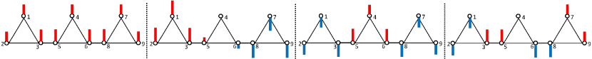
Figure 1. Node embeddings generated by Laplacian Eigenmaps (LE). We show the first four embedding dimensions sequentially (left to right) as bars overlaid on every node. Positive/negative values are denoted by red/blue, and the bar lengths indicate the absolute values. We observe greater fluctuation between neighboring nodes in later dimensions.

Nevertheless, direct application of LE ignores an important characteristic of the KNN graph, that the graph edges are estimated from different amounts of data and hence have unequal variance. If we only observe short interaction history for some users and items, it is difficult to obtain good estimates of their positions (i.e. neighbors) on the data manifold and of their embeddings. As a result, direct application of LE may lead to poor performance.

To address the problem, we propose Laplacian Eigenmaps with Popularity-based Regularization for Isolated Data (Leporid). Leporid regularizes the embeddings based on the observed frequencies of users and items, serving as variance reduction for estimated embeddings. Leporid embeddings can be efficiently solved by using sparse matrix eigendecomposition with known convergence guarantees. Experimental results show that Leporid outperforms existing initialization schemes on a wide range of neural recommender systems, including collaborative filtering, graph neural networks, and sequential recommendation networks. Although randomly initialized neural recommendation methods compare unfavorably with KNN techniques, with Leporid initializations, they often perform on par or better than KNN methods.

To fully realize the strength of Leporid, we propose Dual-Loss Residual Recommendation (DLR²), a simple residual network with two complementary losses. On three real-world datasets, DLR² with Leporid initialization outperforms all baselines by large margins. An ablation study reveals that the use of residual connections contributes significantly to the performance of DLR². Under certain conditions, the output of residual networks contains all information in the input (Behrmann et al., 2019). Thus, the proposed architecture may utilize manifold information throughout the network, improving performance.

With this paper, we make the following contributions:

• Consistent with (Dacrema et al., 2019), we find that randomly initialized neural recommenders perform worse than KNN methods. However, with Leporid initialization, neural recommenders outperform well-tuned KNN methods, underscoring the importance of initialization for neural recommender systems.

• To capture neighborhood structures on the data manifold, we propose to initialize user and item representations with Laplacian Eigenmaps (LE) embeddings. To the best of our knowledge, this is the first work applying LE in initializing neural recommendation systems.

• Further, we identify the issue of high variance in LE embeddings for KNN graphs and propose Popularity-based Regularization for Isolated Data (Leporid) to reduce the variance for users and items on the tail of the data distribution. The resulted Leporid embeddings outperform LE embeddings on all neural recommendation systems that we tested.

• We propose a new network architecture, DLR², which employs residual connections and two complimentary losses to effectively utilize the superior initialization. On three real-world datasets, DLR² initialized by Leporid surpasses all baselines including traditional and proper initialized deep neural networks by large margins.

2. Related Work

2.1. Initializing Neural Networks

Proper initialization is crucial for the optimization and the generalization of deep neural networks. Poor initialization was a major reason that early neural networks did not realize the full potential of first-order optimization (Sutskever et al., 2013). Xavier (Glorot and Bengio, 2010) and Kaiming initializations (He et al., 2015b) are schemes commonly used in convolutional networks. Further highlighting the importance of initialization, recent theoretical developments (Theorems 1 & 2 of (Allen-Zhu et al., 2018); Collorary 4.1 of (Du et al., 2019)) show the point of convergence is close to the initialization. Large pretrained models such as BERT (Devlin et al., 2018) can also be seen as supplying good initialization for transfer learning.

While most neural recommendation systems make use of random initialization, some recent works (He et al., 2017; Zhang et al., 2020a; Liu et al., 2019) initialize embeddings from BPR (Rendle et al., 2009). (Zhu et al., 2020) embeds user and item representations using node2vec (Grover and Leskovec, 2016) on the heterogeneous graph containing both explicit feedback (e.g., ratings) and side information (e.g., user profiles). (Hu et al., 2020a; Zhang et al., 2020b) explore pretraining for graph networks, but they critically rely on side information like visual features of movies.

In comparison, LE and Leporid initialization schemes represent the intrinsic geometry of the data manifold and do not rely on any side information. To the best of our knowledge, this is the first work employing intrinsic geometry based initialization for neural recommendation systems. Experiments show that the proposed initialization schemes outperform a wide range of existing ones such as pretrained embeddings from BPR (Rendle et al., 2009) and Graph-Bert (Zhang et al., 2020b) without side information. In addition, LE and Leporid initializations can be efficiently obtained with established convergence guarantees (see Section 3.4), whereas large pretrained neural networks like (Zhang et al., 2020b) require significantly more computation and careful tuning of hyperparameters for convergence.

2.2. Recommendation Systems

From the aspect of research task, sequential recommendations (Wu et al., 2018; Xu et al., 2019; Tang and Wang, 2018; Kang and McAuley, 2018; Yuan et al., 2018; Wu et al., 2017; Hidasi et al., 2015; Rendle et al., 2019) are recently achieving more research attentions, as the interactions between users and items are essentially sequentially dependent (Wang et al., 2019b). Sequential recommendations explicitly model users’ sequential behaviors.

From the aspect of recommendation techniques, existing methods are mainly based on collaborative filtering (Rendle et al., 2009; Wang et al., 2006; Sarwar et al., 2001) and deep learning (He et al., 2017; Zhang et al., 2020a; Jin et al., 2020). Graph Neural Networks (GNN) have recently gained popularity in recommendation systems (Ying et al., 2018; Qu et al., 2020; Chang et al., 2020). GNN-based recommendation methods (Wu et al., 2020) typically build the graph with users and items as nodes and interactions as edges, and apply aggregation methods on the graph. Most works (Chen and Wong, 2020; Wang et al., 2020b; Qin et al., 2020; Song et al., 2019) make use of spatial graph convolution, which focuses on local message passing. A few works have investigated the use of spectral convolution on the graph (Zheng et al., 2018; Liu et al., 2019).

The initialization schemes we propose are orthogonal to the above works on network architecture. Empirical results demonstrate that the LE and Leporid initialization schemes boost the accuracy of a diverse set of recommendation systems, including GNNs that already employ graph information.

3. Proposed Initialization Schemes

Table 1. Frequently used notations

$\mathcal{D}$	Dimensionality of user and item embeddings
$\mathcal{N}$	Number of nodes in the graph
$G$	Graph used in Laplacian eigenmaps
$W$	Weighted adjacency matrix
$W_{i,j}$	Weight of the edge between nodes $i$ and $j$
$d_{i}$	Degree of node $i$
$d_{\text{max}}$	Maximum degree of the graph
$D$	Diagonal degree matrix
$L$	Unnormalized graph Laplacian
$L_{\text{sym}}$	Normalized symmetric graph Laplacian
$L_{\text{reg}}$	Unnormalized graph Laplacian with popularity-based regularization
$L_{\text{regsym}}$	Normalized symmetric graph Laplacian with popularity-based regularization
$\lambda_{i}$	$i^{\text{th}}$ eigenvalue of the graph Laplacian
$\bm{q}^{(i)}$	$i^{\text{th}}$ eigenvector of the graph Laplacian

3.1. Laplacian Eigenmaps

Given an undirected graph $G=\langle V,E\rangle$ with non-negative edge weights, Laplacian Eigenmaps creates $\mathcal{D}$-dimensional embeddings for the $\mathcal{N}$ graph nodes. We use $W\in\mathbb{R}^{\mathcal{N}\times\mathcal{N}}$ to denote the adjacent matrix, whose entry $W_{i,j}$ is the weight of the edge between nodes $i$ and $j$. $W_{i,j}\geq 0$ and $W_{i,j}=W_{j,i}$. If nodes $i$ and $j$ are not connected, $W_{i,j}=W_{j,i}=0$. The degree of node $i$, $d_{i}=\sum_{j}W_{i,j}$, is the sum of the weights of edges adjacent to $i$. The degree matrix $D\in\mathbb{R}^{\mathcal{N}\times\mathcal{N}}$ has $d_{i}$ on its diagonal, $D_{i,i}=d_{i}$, and zero everywhere else. The unnormalized graph Laplacian is defined as

(1) $$L=D-W.$$

$L$ is positive semi-definite (PSD) since for all $\bm{q}\in\mathbb{R}^{\mathcal{N}}$,

(2) $$\bm{q}^{\top}L\bm{q}=\frac{1}{2}\sum_{i}\sum_{j}W_{i,j}(q_{i}-q_{j})^{2}\geq 0,$$

where $q_{i}$ refers to the $i^{th}$ component of $\bm{q}$. Alternatively, we may use the normalized symmetric graph Laplacian $L_{\text{sym}}$ (Chung, 1997; Ng et al., 2001),

(3) $$L_{\text{sym}}=D^{-\frac{1}{2}}(D-W)D^{-\frac{1}{2}}.$$

To find node embeddings, we compute the eigendecomposition $L=Q\Lambda Q^{\top}$, where the column of matrix $Q$ are the eigenvectors $\bm{q}^{(1)},\ldots,\bm{q}^{(\mathcal{N})}$ and matrix $\Lambda$ has the eigenvalues $0=\lambda_{1}\leq\lambda_{2}\leq\ldots\leq\lambda_{\mathcal{N}}$ on the diagonal. We select the eigenvectors corresponding to the smallest $\mathcal{D}$ eigenvalues as matrix $\tilde{Q}\in\mathbb{R}^{\mathcal{N}\times\mathcal{D}}$. The rows of $\tilde{Q}$ become the embeddings of the graph nodes. Typically we set $\mathcal{D}\ll\mathcal{N}$.

We can think of $q^{(k)}_{j}$, the $j^{\text{th}}$ component of $\bm{q}^{(k)}$, as assigning a value to the graph node $j$. When $\lambda_{k}$ is small, for adjacent nodes $i$ and $j$, the difference between $q^{(k)}_{i}$ and $q^{(k)}_{j}$ is small. As $\lambda_{k}$ increases, the $k^{\text{th}}$ embedding dimension vary more quickly across the graph (see Figure 1). The resulted embeddings represent multi-scale neighborhood information.

With $L$ being PSD, LE can be understood as solving a sequence of minimization problems. The eigenvectors $\bm{q}^{(1)},\ldots,\bm{q}^{(\mathcal{D})}$ are solutions of the constrained minimization

(4) $$\bm{q}^{(k)}=\operatorname*{arg\,min}_{\bm{q}^{()}}\frac{1}{2}\sum_{i}\sum_{j}W_{i,j}(q_{i}-q_{j})^{2}\\$$

(5) $$\text{s.t. \, }\bm{q}^{()}{}^{\top}\bm{q}^{()}=1\text{\, and \,}\bm{q}^{\top}\bm{q}^{(l)}=0,\forall l<k.$$

We emphasize that, different from the optimization of non-convex neural networks, the LE optimization can be solved efficiently using eigendecomposition with known convergence guarantees (see Section 3.4).

3.2. Popularity-based Regularization

We generate user embeddings from the KNN graph where nodes represent users and two users are connected if one is among the K nearest neighbors of the other. Item embeddings are generated similarly. An important observation is that we do not always have sufficient data to estimate the graph edges well. For nodes on the tail of the data distributions (users or items in nearly cold-start situations), it is highly likely that their edge sets are incomplete.

We empirically characterize the phenomenon by generating random Barabasi-Albert graphs (Albert and Barabási, 2002) and adding one extra edge to nodes with different degrees. We then compute the change in embedding norms caused by the addition, which is averaged over 50 random graphs. For every node on a graph, we randomly pick one edge from all possible new adjacent edges and add it to the graph. This procedure is repeated 30 times for every node. Figure 2 plots the change in norm versus the degree of the node before the addition. Graph nodes with fewer adjacent edges experience more drastic changes in their LE embeddings. This indicates that the LE embeddings for relatively isolated nodes are unreliable because a single missing edge can cause large changes.

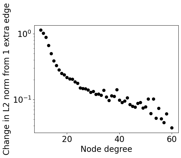
Figure 2. Graph nodes with fewer adjacent edges experience more drastic changes in their LE embeddings when one adjacent edge is added to the node. The y-axis shows the change in the $\ell_{2}$ norm of the embedding of the node. The x-axis shows the node degree before the addition.

As a remedy, we propose Leporid, which selectively regularizes the embeddings of graph node $i$ when $d_{i}$ is small. Keeping the constraints in Eq. 5 unchanged, we replace Eq. 4 with

(6) $$\bm{q}^{(k)}=\operatorname*{arg\,min}_{\bm{q}^{()}}\frac{1}{2}\sum_{i}\sum_{j}W_{i,j}(q_{i}-q_{j})^{2}+\alpha\sum_{i}(d_{\text{max}}-d_{i})q_{i}^{2},$$

where $d_{\text{max}}=\max_{i}d_{i}$ is the maximum degree of all nodes and $\alpha$ is a regularization coefficient. The $(d_{\text{max}}-d_{i})q_{i}^{2}$ term applies stronger regularization to $q_{i}$ as $d_{i}$ decreases. In matrix form,

(7) $$\bm{q}^{(k)}=\operatorname*{arg\,min}_{\bm{q}^{()}}\bm{q}^{()}{}^{\top}L_{\text{reg}}\bm{q}^{()}=\operatorname*{arg\,min}_{\bm{q}^{()}}\bm{q}^{()}{}^{\top}((1-\alpha)D-W+\alpha d_{\text{max}}I)\bm{q}^{()}.$$

As $d_{\text{max}}\geq d_{i}$, $L_{\text{reg}}$ remains PSD, so we can solve the sequential optimization using eigendecomposition as before. For the normalized Laplacian, with $D_{\text{reg}}=(1-\alpha)D+\alpha d_{\text{max}}I$, we perform eigendecomposition on $L_{\text{regsym}}$,

(8) $$L_{\text{regsym}}=D_{\text{reg}}^{-\frac{1}{2}}(D_{\text{reg}}-W)D_{\text{reg}}^{-\frac{1}{2}}.$$

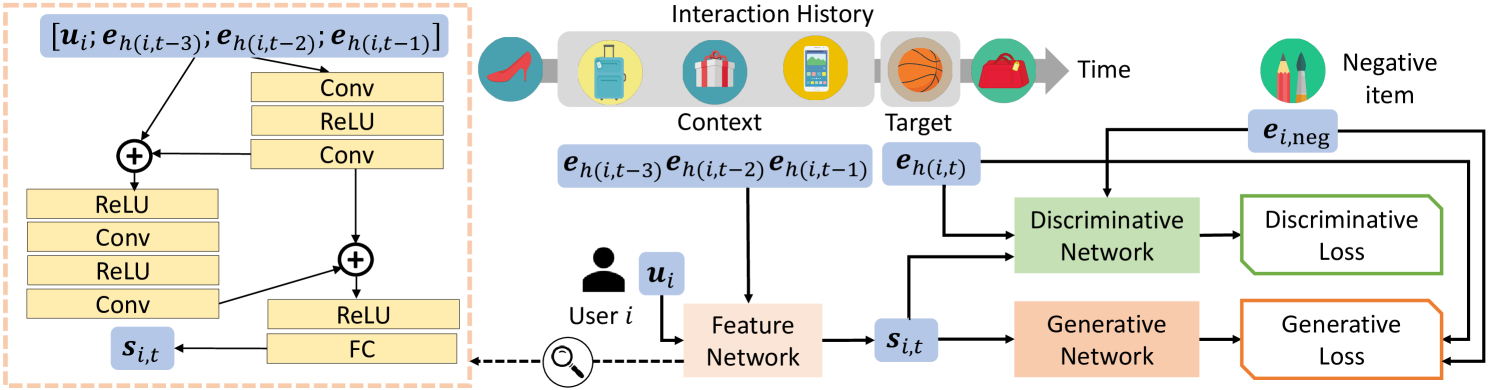
Figure 3. The network architecture, including the Feature Network, which feeds into two branches: the Discriminative Network and the Generative Network. The Feature Network utilizes the residual structure in the box on the left.

To see the rationale behind the proposed technique, note that minimizing Eq. 4 will set the components $q_{i}$ and $q_{j}$ as close as possible. When the orthogonality constraints require some $q_{i}$ and $q_{j}$ to be different, the optimization makes them unequal only where the non-negative weight $W_{i,j}$ is small. When a node $i$ has small degree $d_{i}$, most of its $W_{i,j}$ are zero or small, so large changes in $q_{i}$ cause only negligible changes to the minimization objective. The additional regularization term penalizes large values for $q_{i}$, hence achieving regularization effects.

The proposed regularization can also be understood from the probabilistic perspective (Lawrence, 2012). The eigenvector component $q_{i}$, which is associated with node $i$, may be seen as a random variable that we estimate from observations $W$. A small $d_{i}$ indicates that we have limited data for estimating $q_{i}$, resulting in a high variance in the estimates. Had we observed a few additional interactions for such nodes, their embeddings could change drastically. The proposed regularization involving $q_{i}^{2}$ can be understood as a Gaussian prior for $q_{i}$ with adaptive variance.

3.3. KNN Graph Construction

To apply LE and Leporid, we construct two separate similarity graphs respectively for users and items. We will describe the construction of the user graph; item graph is constructed analogously.

Intuitively, two users are similar if they prefer the same items. Thus, we define the similarity between two users as the Jaccard index, or the intersection over union of the sets of items they interacted with (Sun et al., 2017). Letting $\mathcal{I}_{i}$ denote the set of items that user $i$ interacted with, the similarity between user $i$ and user $j$ is

(9) $$\text{sim}(i,j)=\frac{|\mathcal{I}_{i}\cap\mathcal{I}_{j}|}{|\mathcal{I}_{i}\cup\mathcal{I}_{j}|},$$

where $|\cdot|$ denotes the set cardinality. In the constructed graph $G$, we set $W_{i,j}=\text{sim}(i,j)$ if user $j$ is among the $K$ nearest neighbors of user $i$, or if user $i$ is among the $K$ nearest neighbors of user $j$. Otherwise, $W_{i,j}=0$.

3.4. Computational Complexity

Eigenvalue decomposition that solves for LE and Leporid embeddings has a high time complexity of $O(\mathcal{N}^{3})$ for a graph with $\mathcal{N}$ nodes, which does not scale well to large datasets. Fortunately, for the $K$ nearest neighbor graph, the graph Laplacian is a sparse matrix with the sparsity larger than $1-\frac{2K^{2}}{\mathcal{N}^{2}}$. Utilizing this property, the Implicit Restarted Lanczos Method (IRLM) (Lehoucq and Sorensen, 1996; Hou et al., 2018) computes the first $\mathcal{D}$ eigenvectors and eigenvalues with time complexity $O(K^{2}\mathcal{D}\kappa)$, where $\kappa$ is the conditional number of $L$. Note that this complexity is independent of $\mathcal{N}$. In our experiment, it took only 172 seconds to compute 64 eigenvectors for the user KNN graph of the Anime dataset, which has a $47143\times 47143$ matrix and data sparsity of $96.85$%. In comparison, it took 1888 seconds for the simple BPR model (Rendle et al., 2009) to converge. The experiments were completed using two Intel Xeon 4114 CPUs.

4. Proposed Recommendation Model

To maximize the benefits of the proposed initialization schemes, we design Dual-Loss Residual Recommendation (DLR²). Our preliminary experiments indicate that the immediate interaction history has the most predictive power for the next item that the user will interact with. For this reason, we select the last few items the user interacted with and the user embedding as the input features to the model. In the recommender system literature, this is known as sequential recommendation (Wang et al., 2019b). It is worth noting that LE and Leporid embeddings provide performance enhancement in a wide range of recommender systems, even though their effects are the most pronounced in sequential recommendation.

We denote the embeddings for user $i$ as $\bm{u}_{i}\in\mathbb{R}^{\mathcal{D}}$ and the embedding for item $j$ as $\bm{e}_{j}\in\mathbb{R}^{\mathcal{D}}$. After initialization, the embeddings are trained together with other network parameters. $h(i,t)$ denotes the item that user $i$ interacted with at time $t$. In order to represent the short-term interest of user $i$ at time $t$, we select the most recent $l$ items in the interaction history as $\bm{r}_{i,t}=[\bm{e}_{h(i,t-l-1)};\ldots;\bm{e}_{h(i,t-1)}]$.

The network architecture is displayed in Figure 3. The Feature Network takes $\bm{r}_{i,t}$ and $\bm{u}_{i}$ as input and outputs a common feature representation $\bm{s}_{i,t}\in\mathbb{R}^{\mathcal{D}}$. We employ residual connections (He et al., 2015a) in the Feature Network. Letting $x$ denote the input to a residual block, we feed $x$ into two convolution layers whose output is $F(x)$. The output of the block is $H(x)=F(x)+x$. We employ two residual blocks in the Feature Network, followed by a fully connected layer.

Residual connections may create invertible outputs (Behrmann et al., 2019), which preserve all the information in the input embeddings. We hypothesize that this may allow the network to fully utilize the power of initialization and put the hypothesis to test in Section 5.5.4.

We feed the acquired feature $\bm{s}_{i,t}$ into both the Discriminative Network and the Generative Network, which exploit complementary aspects of the supervision. The Discriminative Network $\mathcal{S}$ evaluates the preference of the user $i$ towards item $j$ at time $t$. We feed the user’s current state $\bm{s}_{i,t}$ and the item embedding $\bm{e}_{j}$ into $\mathcal{S}$. The output $\mathcal{S}(\bm{s}_{i,t},\bm{e}_{j})\in\mathbb{R}$ represents the distance between users’ preference and item $j$. More specifically, lower output value indicates higher similarity and better preference. We apply the square-square loss that suppresses the output distance of the correct item $\bm{e}_{h(i,t)}$ toward 0 and lifts the distance of a randomly sampled negative item $\bm{e}_{i,neg}$ above a margin $m_{S}$,

(10) $$\begin{split}\mathcal{L}_{S}&=\mathbb{E}\biggl{[}\mathcal{S}(\bm{s}_{i,t},\bm{e}_{h(i,t)})^{2}+\left(\max(m_{S}-\mathcal{S}(\bm{s}_{i,t},\bm{e}_{i,neg}),0)\right)^{2}\biggr{]},\end{split}$$

where $\mathbb{E}$ is the expectation over $i,t$ and negative samples.

The Generative Network $\mathcal{G}$ directly predicts the embedding of items that the user prefers. Its output is $\mathcal{G}(\bm{s}_{i,t})\in\mathbb{R}^{\mathcal{D}}$. We employ Euclidean distance to estimate the similarity between the network output $\mathcal{G}(\bm{s}_{i,t})\in\mathbb{R}^{\mathcal{D}}$ and the evaluated item. The goal is to make the distance of the correct item $\bm{e}_{h(i,t)}$ smaller than the distance of the randomly sampled negative item $\bm{e}_{i,neg}$. We adopt the following hinge loss with margin $m_{G}$,

(11) $$\begin{split}\mathcal{L}_{G}&=\mathbb{E}\biggl{[}\max(\|\mathcal{G}(\bm{s}_{i,t})-\bm{e}_{h(i,t)}\|_{2}-\|\mathcal{G}(\bm{s}_{i,t})-\bm{e}_{i,neg}\|_{2}+m_{G},0)\biggr{]}.\end{split}$$

The final loss of the network is the sum of $\mathcal{L}_{G}$ and $\mathcal{L}_{S}$, which describe different aspects of supervisory signals.

5. Experiments

5.1. Datasets

Table 2. Dataset Statistics. Tail users and items are defined as the 25% of users and items with the least interaction records. Their data shares are the proportions of their interactions out of all interaction records.

Datasets	#Users	#Items	# Inter- actions	Data Density	Tail Users’ Data Share	Tail Items’ Data Share
ML-1M	6,040	3,650	1,000,127	4.54%	4.51%	1.08%
Steam	33,699	6,253	1,470,329	0.70%	11.67%	1.83%
Anime	47,143	6,535	6,143,751	1.99%	5.73%	0.93%

The proposed algorithm is evaluated on three real-world datasets from different domains: MovieLens-1M (ML-1M) (Harper and Konstan, 2015), Steam, and Anime. Table 2 shows the dataset statistics. Among the three datasets, Steam is the most sparse with data sparsity over 99.3%. We split the datasets according to the time of interaction; the first 70% interaction history of each user is used as the training set, the next 10% as the validation set, and the rest as the testing set. For all three datasets, we retain only users and items with at least 20 interactions. When creating the candidate items for each user during testing, we use only items that the user has not interacted with in the training set or the validation set.

5.2. Initialization Methods

We select a comprehensive list of initialization methods, including traditional initialization and state-of-the-art pre-training methods.

• Random embeddings drawn i.i.d. from a Gaussian distribution with zero mean and standard deviation 0.01.

• SVD, or singular value decomposition of the user-item interaction matrix $T\in\mathbb{R}^{N\times M}$. Let $T=U\Sigma V^{\top}$ and $\tilde{\Sigma}$ denote the diagonal matrix with the largest $\mathcal{D}$ singular values. The user and item embeddings are $U\tilde{\Sigma}^{\frac{1}{2}}$ and $\tilde{\Sigma}^{\frac{1}{2}}V^{\top}$ respectively.

• BPR (Rendle et al., 2009), which ranks items based on the inner product of user and item embeddings. We take the trained embeddings as initialization for other models.

• NetMF (Qiu et al., 2017), which generalizes a variety of skip-gram models of graph embeddings such as DeepWalk (Perozzi et al., 2014), LINE (Tang et al., 2015b), PTE (Tang et al., 2015a) and node2vec (Grover and Leskovec, 2016). NetMF empirically outperforms DeepWalk and LINE in conventional network mining tasks.

• node2vec (Grover and Leskovec, 2016). Following (Zhu et al., 2020), we trained node2vec on the heterogeneous graph with users and items as nodes and user-item interactions as edges. However, due to its high time complexity and high memory consumption (Pimentel et al., 2018), we are unable to compute node2vec embeddings on Anime.

• Graph-Bert (Zhang et al., 2020b), the user and item embeddings from Graph-Bert pretrained with self-supervised objectives. For fair comparisons with methods that do not use side information, we generate node attributes randomly.

For LE and Leporid embeddings, we employ the symmetrically normalized graph Laplacians ($L_{\text{sym}}$ in Eq. 3 and $L_{\text{regsym}}$ in Eq. 8).

Table 3. Performances of different initialization for different neural recommendation methods. The best initialization results of each model are in bold faces and the second best results are underlined. “Relative Imp.” refers to the relative improvement of Leporid over the best baseline (other than LE), which is marked with ^∗.

Methods	Initialization	Dataset: ML-1M				Dataset: Steam				Dataset: Anime
		HR@5	HR@10	F1@5	F1@10	HR@5	HR@10	F1@5	F1@10	HR@5	HR@10	F1@5	F1@10
NCF	random	0.0525	0.0874	0.0027	0.0044	0.0036	0.0090	0.0005	0.0009	0.0481	0.0591	0.0036	0.0037
	SVD	0.2980∗	0.4669∗	0.0311∗	0.0512∗	0.0791	0.1557	0.0130	0.0203	0.0513	0.0892	0.0047	0.0081
	BPR	0.2634	0.4096	0.0234	0.0388	0.0995∗	0.1984	0.0166∗	0.0269∗	0.0490	0.0814	0.0044	0.0075
	NetMF	0.2151	0.3505	0.0180	0.0313	0.0912	0.2012∗	0.0147	0.0267	0.0540	0.0910	0.0050∗	0.0084∗
	node2vec	0.2321	0.3776	0.0199	0.0340	0.0748	0.1475	0.0127	0.0196	–	–	–	–
	Graph-Bert	0.1406	0.2354	0.0086	0.0154	0.0823	0.1577	0.0133	0.0196	0.0596∗	0.1044∗	0.0041	0.0073
	LE	0.2422	0.3916	0.0219	0.0369	0.0893	0.1766	0.0143	0.0229	0.0612	0.1013	0.0051	0.0088
	Leporid	0.3262	0.4515	0.0311	0.0561	0.1027	0.2025	0.0167	0.0269	0.0678	0.1111	0.0054	0.0094
Relative Imp.		9.46%	-3.30%	-0.02%	9.49%	3.22%	0.65%	0.70%	-0.20%	13.76%	6.42%	7.71%	12.82%
NGCF	random	0.0725	0.1343	0.0039	0.0070	0.1072	0.1750	0.0179	0.0227	0.1789	0.3023	0.0253	0.0376
	SVD	0.3164	0.4674	0.0360	0.0549	0.1050	0.1752	0.0175	0.0226	0.3585∗	0.5186∗	0.0461∗	0.0607∗
	BPR	0.3301∗	0.4815∗	0.0420∗	0.0647∗	0.1071	0.1747	0.0179	0.0226	0.1719	0.2849	0.0338	0.0450
	NetMF	0.2873	0.4272	0.0297	0.0481	0.1016	0.1699	0.0173	0.0220	0.2355	0.3798	0.0342	0.0512
	node2vec	0.3195	0.4699	0.0369	0.0573	0.1193∗	0.1939∗	0.0205∗	0.0255∗	–	–	–	–
	Graph-Bert	0.3169	0.4654	0.0354	0.0531	0.0980	0.1621	0.0161	0.0206	0.0847	0.1559	0.0059	0.0103
	LE	0.3525	0.5070	0.0436	0.0679	0.1102	0.1818	0.0184	0.0238	0.3739	0.5270	0.0496	0.0760
	Leporid	0.3785	0.5258	0.0439	0.0667	0.1342	0.2084	0.0228	0.0277	0.5098	0.6401	0.0712	0.1014
Relative Imp.		14.66%	9.20%	4.66%	3.09%	12.49%	7.48%	11.21%	8.90%	42.20%	23.43%	54.56%	67.02%
DGCF	random	0.3505	0.4964	0.0395	0.0611	0.1510	0.2321	0.0262	0.0317	0.2973	0.4474	0.0432	0.0618
	SVD	0.3530	0.4982∗	0.0407	0.0635	0.1549	0.2365	0.0270	0.0325	0.3523∗	0.5088∗	0.0483∗	0.0697∗
	BPR	0.3412	0.4964	0.0413	0.0647	0.1515	0.2371	0.0263	0.0320	0.2900	0.4403	0.0413	0.0600
	NetMF	0.3435	0.4977	0.0421∗	0.0650∗	0.1563∗	0.2439∗	0.0274∗	0.0336∗	0.3394	0.4963	0.0467	0.0677
	node2vec	0.3533∗	0.4926	0.0379	0.0597	0.1540	0.2420	0.0265	0.0325	–	–	–	–
	Graph-Bert	0.3483	0.4891	0.0366	0.0592	0.1487	0.2283	0.0256	0.0312	0.2939	0.4494	0.0420	0.0606
	LE	0.3485	0.5032	0.0408	0.0643	0.1551	0.2353	0.0269	0.0320	0.3506	0.5048	0.0488	0.0702
	Leporid	0.3588	0.5045	0.0425	0.0653	0.1661	0.2530	0.0292	0.0349	0.5264	0.6477	0.0679	0.0916
Relative Imp.		1.56%	1.26%	0.97%	0.44%	6.27%	3.73%	6.46%	3.78%	49.42%	27.30%	40.77%	31.50%
HGN	random	0.3270	0.4879	0.0465	0.0688	0.1198	0.1977	0.0205	0.0261	0.1287	0.2457	0.0192	0.0305
	SVD	0.3623	0.5315	0.0536∗	0.0792∗	0.1715∗	0.2594	0.0298∗	0.0358	0.4296∗	0.5989∗	0.0496	0.0764∗
	BPR	0.3377	0.4985	0.0452	0.0688	0.1221	0.2058	0.0205	0.0272	0.2648	0.4070	0.0359	0.0529
	NetMF	0.3806∗	0.5425∗	0.0505	0.0737	0.1479	0.2338	0.0255	0.0318	0.4115	0.5552	0.0514∗	0.0704
	node2vec	0.3649	0.5333	0.0533	0.0783	0.1686	0.2694∗	0.0297	0.0377∗	–	–	–	–
	Graph-Bert	0.2934	0.4379	0.0324	0.0489	0.1304	0.2053	0.0221	0.0270	0.4147	0.5692	0.0506	0.0733
	LE	0.3912	0.5460	0.0507	0.0741	0.1689	0.2524	0.0293	0.0344	0.4753	0.6374	0.0605	0.0875
	Leporid	0.3846	0.5475	0.0543	0.0797	0.1822	0.2745	0.0318	0.0380	0.5010	0.6488	0.0622	0.0902
Relative Imp.		1.05%	0.92%	1.41%	0.70%	6.24%	1.89%	6.75%	0.76%	16.62%	8.33%	21.08%	18.13%
DLR2	random	0.3238	0.4538	0.0310	0.0497	0.1322	0.1912	0.0225	0.0247	0.4191	0.5976	0.0468	0.0744
	SVD	0.4263	0.5820	0.0494	0.0775	0.1275	0.1913	0.0212	0.0241	0.5208	0.6469	0.0626	0.0831
	BPR	0.4750	0.6273	0.0621	0.0979	0.1677 ∗	0.2565∗	0.0290∗	0.0359∗	0.5822∗	0.7167∗	0.0909∗	0.1299∗
	NetMF	0.3969	0.5508	0.0487	0.0770	0.1522	0.2534	0.0260	0.0354	0.5526	0.6795	0.0820	0.1189
	node2vec	0.4947∗	0.6603∗	0.0640∗	0.1011∗	0.1504	0.2408	0.0256	0.0328	–	–	–	–
	Graph-Bert	0.3323	0.4553	0.0308	0.0497	0.1392	0.1976	0.0230	0.0251	0.4100	0.5708	0.0448	0.0700
	LE	0.5119	0.6730	0.0692	0.1070	0.1853	0.2878	0.0332	0.0420	0.6065	0.7438	0.1010	0.1409
	Leporid	0.5406	0.7026	0.0755	0.1158	0.1958	0.2994	0.0352	0.0437	0.6361	0.7654	0.1010	0.1421
Relative Imp.		9.28%	6.41%	18.00%	14.62%	16.76%	16.73%	21.40%	21.68%	9.26%	6.80%	11.08%	9.42%

5.3. Recommendation Baselines

In order to estimate the effectiveness of our initialization methods, we select a comprehensive list of neural recommendation methods, including general collaborative filtering methods, NCF (He et al., 2017), graph convolution methods, NGCF (Wang et al., 2019a) and DGCF (Wang et al., 2020a), and sequential recommendation methods, HGN (Ma et al., 2019) and our proposed DLR².

We also compare our recommendation model DLR² to traditional recommendation methods used in (Dacrema et al., 2019), including the non-personalized method, TopPop, which always recommends the most popular item. We also include traditional KNN approaches (UserKNN (Sarwar et al., 2001) and ItemKNN (Wang et al., 2006)) and matrix factorization approaches (BPR (Rendle et al., 2009) and SLIM (Ning and Karypis, 2011)). Among the traditional baselines in (Dacrema et al., 2019), we find P³$\alpha$ and RP³$\alpha$ to consistently underperform in all experiments and opt not to include them due to space limits. Experimental settings of these models can be found in the Appendix.

Table 4. Performances of different algorithms. The best results of all are in bold faces and the second best results are underlined. The best results of the group above are marked with ^∗. Relative Imp. indicates to the relative improvement of DLR² with Leporid initialization over the best baseline within the group.

Methods	Initialization	Dataset: ML-1M				Dataset: Steam				Dataset: Anime
		HR@5	HR@10	F1@5	F1@10	HR@5	HR@10	F1@5	F1@10	HR@5	HR@10	F1@5	F1@10
TopPop	–	0.3197	0.4377	0.0335	0.0517	0.1413	0.2306	0.0239	0.0307	0.4091	0.6103	0.0504	0.0807
UserKNN	–	0.3851	0.5419∗	0.0483∗	0.0760 ∗	0.1675	0.2575	0.0292	0.0357	0.4098	0.5899	0.0579	0.0802
ItemKNN	–	0.3868∗	0.5235	0.0462	0.0682	0.1729∗	0.2720∗	0.0309∗	0.0385∗	0.5909∗	0.7431∗	0.0949∗	0.1204∗
SLIM	–	0.3692	0.5253	0.0435	0.0680	0.1671	0.2588	0.0290	0.0354	0.5337	0.7132	0.0684	0.1011
BPR	random	0.0851	0.1581	0.0107	0.0171	0.1582	0.2348	0.0279	0.0338	0.0406	0.0800	0.0074	0.0114
Relative Imp.		39.76%	29.65%	56.18%	52.38%	13.24%	10.07%	13.98%	13.39%	7.65%	3.00%	6.43%	18.04%
BPR	Leporid	0.1094	0.2106	0.0151	0.0247	0.1638	0.2442	0.0293	0.0353	0.0810	0.1455	0.0170	0.0233
NCF	Leporid	0.3262	0.4515	0.0311	0.0561	0.1027	0.2025	0.0167	0.0269	0.0678	0.1111	0.0054	0.0094
NGCF	Leporid	0.3785	0.5258	0.0439	0.0667	0.1342	0.2084	0.0228	0.0277	0.5098	0.6401	0.0712∗	0.1014∗
DGCF	Leporid	0.3588	0.5045	0.0425	0.0653	0.1661	0.2530	0.0292	0.0349	0.5264∗	0.6477	0.0679	0.0916
HGN	Leporid	0.3846 ∗	0.5475∗	0.0543∗	0.0797∗	0.1822∗	0.2745∗	0.0318∗	0.0380∗	0.5010	0.6488∗	0.0622	0.0902
Relative Imp.		40.56%	28.33%	38.98%	45.28%	7.46%	9.07%	10.93%	14.89%	20.84%	17.97%	41.84%	40.20%
DLR2	LE	0.5119	0.6730	0.0692	0.1070	0.1853	0.2878	0.0332	0.0420	0.6065	0.7438	0.1010	0.1409
Relative Imp.		5.61%	4.40%	9.07%	8.26%	5.67%	4.03%	6.29%	3.85%	4.88%	2.90%	0.03%	0.86%
DLR2	Leporid	0.5406	0.7026	0.0755	0.1158	0.1958	0.2994	0.0352	0.0437	0.6361	0.7654	0.1010	0.1421

5.4. Evaluation Metrics

To evaluate Top-N recommended items, we use hit ratio (HR@N) and F1 score (F1@N) at N = 1, 5, 10. Hit ratio intuitively measures whether the test item is present on the top-N list. F1 score is the harmonic mean of the precision and recall, which arguably gives a better measure of the incorrectly classified cases than the accuracy metric. We noticed the same tendency of precision and recall, and list the results only in terms of F1 score due to space limitation.

5.5. Results and Discussion

5.5.1. Comparison of Different Initialization

Table 3 shows the experimental results of different initialization on five different types of neural recommendation methods. We make the following observations. First, the choice of initialization has strong effects on the final performance. For example, for NCF on ML-1M dataset, the F1 scores of Leporid are more than 10 times of random initialization. Second, Leporid consistently achieves the top position on most datasets and metrics; LE is a strong second, finishing in the top two in 32 out of the 60 metrics. For example, on Anime with the NGCF model, LE and Leporid lead the best baseline method by 25.22% and 67.02% respectively in F1@10. In DGCF and DLR², Leporid outperforms all other initialization methods. In other recommender systems, Leporid achieves the best performance in all but 1 or 2 metrics. Third, NGCF and DGCF benefit substantially from Leporid, even though they are GNN methods that already utilize graph information. This suggests Leporid is complementary to common graph networks.

5.5.2. Comparison of Recommendation Models

Table 4 compares traditional recommendation methods, Leporid initialized recommendation methods, and DLR² method with LE and Leporid initialization. Like (Dacrema et al., 2019), we find well-tuned UserKNN and ItemKNN competitive. Among traditional recommendation methods, the two KNN methods claim the top spots on all metrics of all datasets. However, on ML-1M and Steam, Leporid-initialized neural recommendation baselines outperform the KNN methods. Together with the results of (Dacrema et al., 2019), this finding highlights the importance of initialization for recommender systems.

Importantly, DLR² with Leporid initialization outperforms all other methods, including strong traditional models and well-initialized neural recommendation models. For instance, on ML-1M dataset and the F1@10 metric, our method leads traditional methods and neural baselines by 52.38% and 45.28%, respectively.

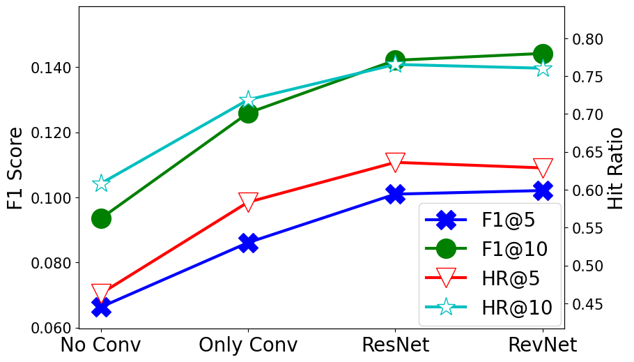
(a) Performance of different architectures in Feature Network in DLR² on Anime dataset, initialized by Leporid.

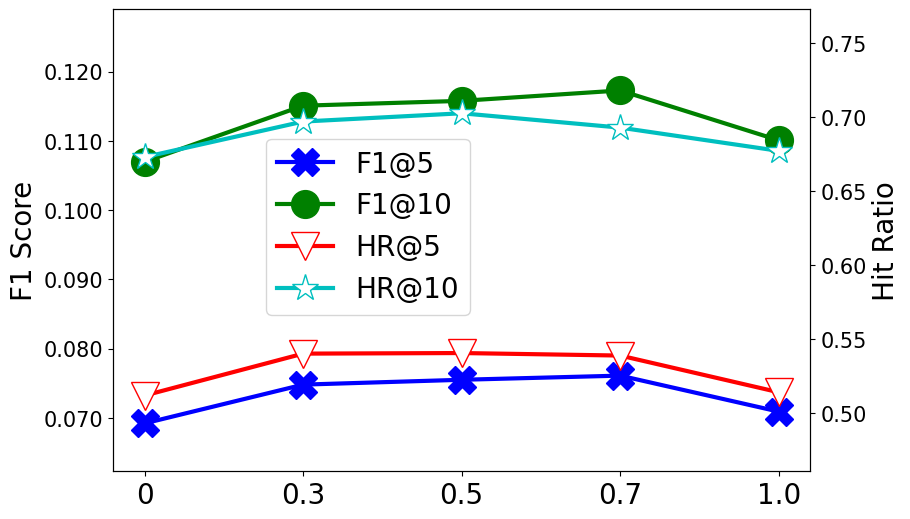
(b) Performance of different regularization coefficient $\alpha$ in Leporid initialization on ML-1M dataset, evaluated on DLR².

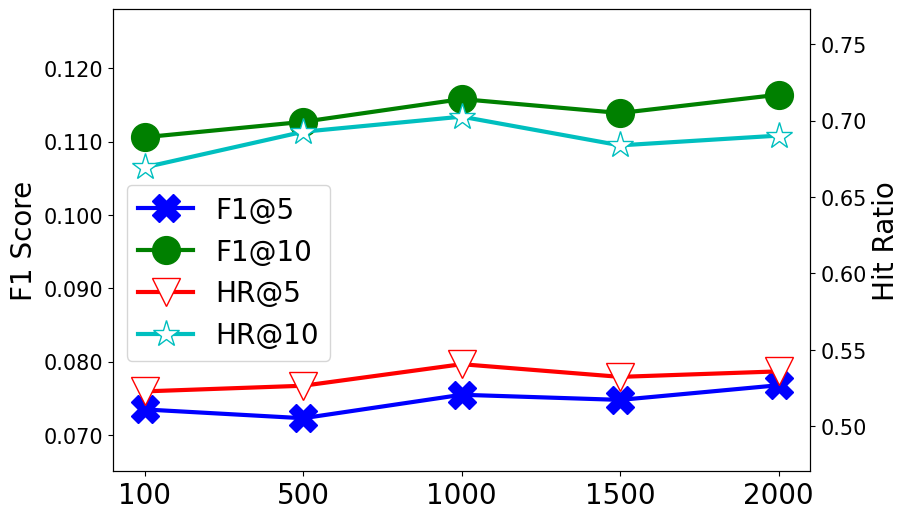
(c) Performance of different neighbor $K$ in Leporid initialization on ML-1M dataset, evaluated on DLR².

Figure 4. Ablation Study

Table 5. Performances of different initialization methods on DLR² on tail users with the least interaction data. “Relative Imp.” refers to the relative improvement of Leporid over the best baseline, including LE.

Dataset	Initialization	HR@5	HR@10	F1@5	F1@10
ML-1M	random	0.1490	0.2490	0.0307	0.0382
	SVD	0.2623	0.4166	0.0558	0.0722
	LE	0.3192	0.4649	0.0724	0.0880
	Leporid	0.3536	0.5159	0.0823	0.1045
	Relative Imp.	10.78%	10.97%	13.67%	18.72%
Steam	random	0.0817	0.1443	0.0177	0.0212
	SVD	0.0704	0.1072	0.0153	0.0155
	LE	0.0973	0.1684	0.0215	0.0258
	Leporid	0.1240	0.2030	0.0284	0.0321
	Relative Imp.	27.44%	20.55%	31.99%	24.44%
Anime	random	0.3209	0.4594	0.0680	0.0732
	SVD	0.2989	0.4661	0.0638	0.0765
	LE	0.3617	0.5205	0.0811	0.0955
	Leporid	0.3953	0.5408	0.0937	0.1195
	Relative Imp.	9.29%	3.90%	15.46%	25.13%

Table 6. Performances of networks trained with different supervision on ML-1M.

Inference Branch	Loss Function	HR@5	HR@10	F1@5	F1@10
$\mathcal{G}$	$\mathcal{L}_{G}$	0.3631	0.4982	0.0427	0.0601
	$\mathcal{L}_{G}+\mathcal{L}_{S}$	0.4955	0.6510	0.0677	0.1012
Relative Imp.		36.46%	30.67%	58.66%	68.41%
$\mathcal{S}$	$\mathcal{L}_{S}$	0.5228	0.6826	0.0744	0.1112
	$\mathcal{L}_{G}+\mathcal{L}_{S}$	0.5406	0.7026	0.0755	0.1158
Relative Imp.		3.40%	2.93%	1.49%	4.19%

5.5.3. Performance on Tail Users

Leporid adaptively regularizes the embeddings of nodes with low degrees, which should benefit users with short interaction histories. In this experiment, we verify that claim by examining model performance on the 25% users with the least interaction records. Selecting all of their interactions yields 9,771, 37,905, and 76,353 records for ML-1M, Steam, and Anime test sets, respectively. We include all items because further exclusion would leave too few data for accurate performance measurement.

We compare the performances of different initialization schemes on DLR² in Table 5. We include SVD initialization because it is the best baseline on the most metrics (20 out of 60) from Table 3. Leporid achieves higher relative performance improvements on tail users than on the entire test sets, as shown in Table 4.

5.5.4. Effects of Architecture Design in DLR²

The simple model of DLR² has achieved the best performance thus far. We now explore architectural factors that contribute to its success. The literature suggests that residual connections may improve the quality of learned representation. In unsupervised learning, (Kolesnikov et al., 2019) finds that residual connections help to maintain the quality of learned representations in CNN throughout the network. (Behrmann et al., 2019) proves that, under certain conditions, the output of residual networks contains all information needed to reconstruct the input. That is, the network is “invertible”. This effect may facilitate DLR² in fully utilizing the strength of the initialization schemes.

We create three variations of DLR² in order to observe the effects of residual connections and invertible representation. “No Conv” replaces all convolutional layers with fully connected layers and has no residual connections. “Only Conv” has convolutional layers but not the residual connections. “ResNet” denotes the complete DLR² model. “RevNet” replaces the convolutional-residual design with the RevNet (Gomez et al., 2017) architecture, which is guaranteed to produce invertible features. Due to space limitation, we only present the results on Anime dataset in Figure 4a. The results on other datasets are similar and can be found in the Appendix.

Observing Figure 4a, we note that both convolutional layers and residual connections lead to significant performance improvements. The RevNet architecture achieves comparable performance with DLR², which suggests that learning invertible representations may facilitate the effective use of good initializations.

5.5.5. Effects of the Two Loss Functions in DLR²

The DLR² model employs a discriminative loss $\mathcal{L}_{S}$ and a generative loss $\mathcal{L}_{G}$. We now examine their effects on the final performance using an ablation study. Table 6 shows the performance when one of the loss functions is removed. When adding $\mathcal{L}_{S}$ to the $\mathcal{L}_{G}$-only network, F1@10 increases relatively by 68.41%. Similarly, adding the $\mathcal{L}_{G}$ branch to the $\mathcal{L}_{S}$-only network improves F1@10 relatively by 4.19%. The results demonstrate that we can harness significant synergy from the two-branch architecture with their respective loss functions.

5.5.6. Sensitivity of Hyperparameters

We analyze the sensitivity of two hyperparameters: the population-based regularization coefficient $\alpha$ in Eq. 8 and the number of nearest neighbors $K$ used to construct the KNN graph. Due to space limitation, we only report the analysis on ML-1M dataset on DLR² model. Figure 4b shows the results when $\alpha$ is selected from $\{0,0.3,0.5,0.7,1.0\}$. We observe that $\alpha=0.7$ achieves the best result. Figure 4c shows the performances of DLR² when the number of the nearest neighbors $K$ is varied. Though higher values of $K$ lead to small improvements, the sensitivity to this hyperparameter is low.

6. Conclusions

In this paper, we propose a novel initialization scheme, Leporid, for neural recommendation systems. Leporid generates embeddings that capture neighborhood structures on the data manifold and adaptively regularize embeddings for tail users and items. We also propose a sequential recommendation model, DLR², to make full use of the Leporid. Extensive experiments on three real-world datasets demonstrate the effectiveness of the proposed initialization strategy and network architecture. We believe Leporid represents one step towards unleashing the full potential of deep neural networks in the area of recommendation systems.

Acknowledgments. This research is supported by the National Research Foundation, Singapore under its AI Singapore Programme (No. AISG-GC-2019-003), NRF Investigatorship (No. NRF-NRFI05-2019-0002), and NRF Fellowship (No. NRF-NRFF13-2021-0006), and by Alibaba Group through the Alibaba Innovative Research (AIR) Program and Alibaba-NTU Singapore Joint Research Institute (JRI).

Appendix A The Optimization of Leporid

Leporid solves the following minimization problem using eigendecomposition of $L_{\text{reg}}=(1-\alpha)D-W+\alpha d_{\text{max}}I$.

(12) $$\begin{split}\bm{q}^{(k)}=&\operatorname*{arg\,min}_{\bm{q}^{()}}\frac{1}{2}\sum_{i}\sum_{j}W_{i,j}(\bm{q}_{i}-\bm{q}_{j})^{2}\\ +&\alpha\sum_{i}(d_{\text{max}}-d_{i})q_{i}^{2}\\ =&\operatorname*{arg\,min}_{\bm{q}^{()}}\bm{q}^{()}{}^{\top}L_{\text{reg}}\bm{q}^{()}\\ \text{s.t. \, }&\bm{q}^{()}{}^{\top}\bm{q}^{()}=1\text{\, and \,}\bm{q}^{\top}\bm{q}^{(l)}=0,\forall l<k.\end{split}$$

In this section, we closely examine the rationale behind this approach.

We start by examining Laplacian Eigenmaps, where the eigenvectors $\bm{q}^{(1)},\ldots,\bm{q}^{(\mathcal{N})}$ can be thought of as solutions of the constrained minimization

(13) $$\begin{split}\bm{q}^{(k)}=&\operatorname*{arg\,min}_{\bm{q}^{()}}\bm{q}^{()}{}^{\top}L\bm{q}^{()}\\ =&\operatorname*{arg\,min}_{\bm{q}^{()}}\bm{q}^{()}{}^{\top}(D-W)\bm{q}^{()}\\ =&\operatorname*{arg\,min}_{\bm{q}^{()}}\frac{1}{2}\sum_{i}\sum_{j}W_{i,j}(\bm{q}_{i}-\bm{q}_{j})^{2}\\ \text{s.t. \, }&\bm{q}^{()}{}^{\top}\bm{q}^{()}=1\text{\, and \,}\bm{q}^{\top}\bm{q}^{(l)}=0,\forall l<k.\end{split}$$

Lemma A.1.

The eigenvectors of the graph Laplacian, $L=D-W$, are the solutions of the constrained minimization problem described by Eq. 13.

Proof.

We aim to find a sequence of solutions $\bm{y}^{(1)},\ldots,\bm{y}^{(\mathcal{N})}$ as solutions to the constrained optimization problem described by Eq. 13.

Since the graph Laplacian $L$ is positive semi-definite, it has real-valued eigenvalues ($0\leq\lambda_{1}\leq\lambda_{2}\leq\cdots\leq\lambda_{\mathcal{N}}$). $L$ is also symmetric, so we can perform the eigendecomposition

(14) $$L=Q^{\top}\Lambda Q,$$

where $\Lambda=\text{diag}(\lambda_{1},\lambda_{2},\cdots,\lambda_{\mathcal{N}})$ is a diagonal matrix with the eigenvalues on its diagonal. $Q$ is the orthogonal matrix composed of eigenvectors, $\bm{q}^{(1)},\ldots,\bm{q}^{(\mathcal{N})}$, as its rows, and $Q^{-1}=Q^{\top}$.

We can denote the minimization objective as $R(\bm{x})$,

(15) $$R(\bm{x})=\bm{x}^{\top}L\bm{x}=(Q\bm{x})^{\top}\Lambda(Q\bm{x}).$$

For any $\bm{y}\in\mathbb{R}^{\mathcal{N}}$, we can find $\bm{x}=Q\bm{y}$ such that $Q^{\top}\bm{x}=\bm{y}$:

(16) $$R(\bm{y}) =(Q\bm{y})^{\top}\Lambda(Q\bm{y})$$

$$=(QQ^{\top}\bm{x})^{\top}\Lambda(QQ^{\top}\bm{x})$$

$$=\bm{x}^{\top}\Lambda\bm{x}$$

$$=\lambda_{1}\bm{x}_{1}^{2}+\lambda_{2}\bm{x}_{2}^{2}+\cdots+\lambda_{n}\bm{x}_{n}^{2}.$$

From the constraint $\bm{y}^{\top}\bm{y}=1$, it is easy to see that $\bm{x}^{\top}\bm{x}=1$. Recall that the eigenvalues are arranged in ascending order

(17) $$0\leq\lambda_{1}\leq\lambda_{2}\leq\ldots\leq\lambda_{\mathcal{N}}.$$

To minimize $R(\bm{y})$, we just need to allocate the norm of $\bm{x}$ entirely to the its first component, resulting in $\bm{x}^{(1)}=[1,0,\ldots,0]^{\top}$. Hence, the corresponding $\bm{y}^{(1)}=Q^{\top}\bm{x}^{(1)}$ is the first eigenvector $\bm{q}^{(1)}$. The minimum is $R(\bm{y}^{(1)})=\lambda_{1}$.

From the second solution onward, we have the additional constraints that $\bm{y}^{(k)\top}\bm{y}^{(l)}=0,\forall l<k$. Plugging in $\bm{y}^{(k)}=Q^{\top}\bm{x}^{(k)}$, we can see orthogonality in $\bm{y}$ implies orthogonality in $\bm{x}$: $\bm{x}^{(k)\top}\bm{x}^{(l)}=0,\forall l<k$. To find $\bm{x}^{(2)}$ that is orthogonal to the first solution $\bm{x}^{(1)}$, we just need to set its first component to 0. Hence, the minimizing solution $\bm{x}^{(2)}=[0,1,0,\ldots,0]^{\top}$ and $\bm{y}^{(2)}=\bm{q}^{(2)}$.

Repeating the above steps, we can show the eigenvectors $\bm{q}^{(1)},\ldots,\bm{q}^{(\mathcal{N})}$ are the solutions to the constrained minimization problem. ∎

Theorem A.2.

The eigenvectors of the regularized graph Laplacian, $L_{\text{reg}}$, are the solutions of the constrained minimization problem described by Eq. 12.

Proof.

Because $d_{max}=\max(d_{i}\in D)$, the regularized graph Laplacian, $L_{\text{reg}}$, remains positive semi-definite. Applying the same proof in Lemma A.1, the eigenvectors of $L_{\text{reg}}$ are the solutions for the constrained minimization problem described by Eq. 12. ∎

Table 7. Performances of different recommendation architectures. The best results are in bold faces and the second best results are underlined.

Methods	Dataset: ML-1M				Dataset: Steam				Dataset: Anime
	HR@5	HR@10	F1@5	F1@10	HR@5	HR@10	F1@5	F1@10	HR@5	HR@10	F1@5	F1@10
NO conv	0.4331	0.5781	0.0539	0.0815	0.1729	0.2667	0.0301	0.0380	0.4627	0.6081	0.0663	0.0935
ONLY conv	0.5088	0.6728	0.0718	0.1101	0.1777	0.2755	0.0313	0.0395	0.5835	0.7187	0.0861	0.1259
ResNet	0.5406	0.7026	0.0755	0.1158	0.1958	0.2994	0.0352	0.0437	0.6361	0.7654	0.1010	0.1421
RevNet	0.5394	0.6965	0.0766	0.1162	0.1962	0.3023	0.0353	0.0443	0.6288	0.7604	0.1021	0.1442

Appendix B Performances of Different Architecture Designs in DLR²

Table 7 summarizes the experimental results of different architecture designs in DLR², on ML-1M, Steam and Anime datsets.

Appendix C Reproducibility: Time Cost

For eigen decomposition of both LE and Leporid initialization schemes, we use the package of “scipy.sparse.linalg.eigs”, which is an implementation of IRLM method (Lehoucq and Sorensen, 1996; Hou et al., 2018). However, IRLM method is proposed for computing the first several largest eigenvalues. We shift the initial matrix $W$ using $W^{\prime}=\lambda I-W$, where $\lambda=\max(W)$. The result is averaged over 3 repeated experiments.

Appendix D Reproducibility: Random Seed

Readers may replicate the results reported in the paper using the random seed of 123.

Appendix E Reproducibility: The Simulation in Figure 2

The simulation aims to find the change in the embeddings of nodes when one additional edge is attached to it. To do so, it gathers statistics from 50 random Barabasi-Albert graphs (Albert and Barabási, 2002) using the NetworkX library. The algorithm starts from an initial graph with $m_{0}$ nodes and no edges and gradually adds nodes and random edges until the graph contains $n$ nodes. Here $m_{0}=10$ and $n=100$.

In every random graph, we pick one random node and add a random edge to it. We compute 40-dimensional embedding for that node before and after the addition using Laplacian Eigenmaps. We then compute the $\ell_{2}$ norm of the change in the embeddings. We perform 30 independent edge insertions for every node in the graph, and record the degree of the node before the addition and the average $\ell_{2}$ norm. The statistics are averaged again over 50 random graphs.

Note the random Barabasi-Albert graphs thus generated have very few nodes with degrees less than 10 or greater than 60. That is why the x-axis in Figure 1 starts at 10 and ends at 60.

Appendix F Reproducibility: Experimental Settings of Initialization Schemes

The output embedding size for all initialization schemes is set to $64$. Specifically, in BPR (Rendle et al., 2009), regularization coefficients for both users and items are set to $0.1$ and the coefficient for gradient update is set to $0.25$. NetMF (Qiu et al., 2017) is implemented using a large window size (i.e., 10), which usually performs better than using a small window size (i.e., 1). In node2vec (Grover and Leskovec, 2016) initialization scheme, the length of walking per source is set to $80$ and number of walks is set to $10$. In Graph-Bert (Zhang et al., 2020b), we utilize the network structure recovery as the pre-training task since the node attributes are randomly generated in our experiments.

In the KNN graphs, which is the input for NetMF, LE and Leporid, the number of nearest neighbors $K$ is set to 1000. The regularization coefficient $\alpha$ in Leporid is set to $0.5$.

Appendix G Reproducibility: Experimental Settings of Recommendation Methods

The embedding size for all neural recommendation models (i.e., NCF (He et al., 2017), NGCF (Wang et al., 2019a), DGCF (Wang et al., 2020a), HGN (Ma et al., 2019) and our proposed DLR²) is set to $64$. Other hyperparameters like learning rate and the number of training steps are tuned by grid search on the validation set. The initial learning rate is selected from the range $[0.0001,0.01]$ and weight decay is selected from the range $[0,0.01]$. We use Adam (Kingma and Ba, 2015) for training all neural recommendation methods.

Specifically, in DLR², the number of recent items, $l$, is set to $5$. In Feature Network, we employ two similar residual connections. In the first residual block, we have two convolutional layers (kernel size = 3, stride = 1, output channel size = 64), activated by ReLU. In the second block, we employ convolutional layers (kernel size = 3, stride = 2, output channel size = 128) and add downsampling (convolutional layers where kernel size = 1, stride = 2) to the initial input to match the size.

The Generative Network $\mathcal{G}$ and Discriminative Network $\mathcal{S}$ are implemented with the same network structure except the final layer, which consists of three fully connected neural layers (output sizes of each layer are $[256,256,128]$ respectively), activated by ReLU. In $\mathcal{G}$, we use Tanh as the activation function in the final layer (output size = $64$). $\mathcal{S}$ is activated by ReLU in the final layer (output size = $1$). We set both margins in Eq. 10 and Eq. 11 as 0, that is, $m_{S}=m_{G}=0$. We use the sum of $\mathcal{L}_{S}$ and $\mathcal{L}_{G}$ for training and select the Discriminative Network for evaluation in Table 3 and Table 4.

Other traditional recommendation methods (i.e., TopPop, UserKNN (Sarwar et al., 2001), ItemKNN (Wang et al., 2006), SLIM (Ning and Karypis, 2011)) are implemented following the work of (Dacrema et al., 2019).

Appendix H Reproducibility: Experimental Settings of Different Architecture Designs

In Section 5.5.4, which explores the effect of residual connections in Feature Network in DLR², the settings of different architectures are as follows. “No Conv” replace the residual connections with four fully connected layers, where the output sizes for each layer are[256, 256, 256, 256]. “Only Conv” includes simple convolutional layers and other parameters are the same as the “ResNet”, which is described in Appendix G. “RevNet” replaces previous residual connections with modified ones. It first splits the input $x$ channel-wise into two equal parts $x_{1}$ and $x_{2}$. The output is then the concatenation of $y_{1}=x_{1}+F(x_{2})$ and $y2=x2+G(y_{1})$. Both $F(\cdot)$ and $G(\cdot)$ includes two convolutional layers, activated by ReLU. We add additional one convolutional layer (kernel size = 3, stride = 2, output channel size = 128) between the two modified residual blocks and other parameters are the same to the “ResNet” architecture.

Appendix I Reproducibility: Experimental Settings of Hyperparameter Study

In Section 5.5.6, which study the sensitivity of hyperparameters in building Leporid initialization, we keep other parameters unchanged. In other words, we set nearest neighbor $K=1000$ in Figure 4b and set regularization coefficient $\alpha=0.5$ in Figure 4c.

References

- (1)
- Albert and Barabási (2002) Réka Albert and Albert-László Barabási. 2002. Statistical mechanics of complex networks. Reviews of Modern Physics (2002).
- Allen-Zhu et al. (2018) Zeyuan Allen-Zhu, Yuanzhi Li, and Zhao Song. 2018. A Convergence Theory for Deep Learning via Over-Parameterization. arXiv 1811.03962 (2018).
- Behrmann et al. (2019) Jens Behrmann, Will Grathwohl, Ricky T. Q. Chen, David Duvenaud, and Jörn-Henrik Jacobsen. 2019. Invertible Residual Networks. In ICML.
- Belkin and Niyogi (2003) M. Belkin and P. Niyogi. 2003. Laplacian Eigenmaps for Dimensionality Reduction and Data Representation. Neural Computation (2003).
- Chang et al. (2020) Jianxin Chang, Chen Gao, Xiangnan He, Depeng Jin, and Yong Li. 2020. Bundle Recommendation with Graph Convolutional Networks. In SIGIR.
- Chen and Wong (2020) Tianwen Chen and Raymond Chi-Wing Wong. 2020. Handling Information Loss of Graph Neural Networks for Session-Based Recommendation. In KDD.
- Chung (1997) F. R. K. Chung. 1997. Spectral Graph Theory. American Mathematical Society.
- Dacrema et al. (2019) Maurizio Ferrari Dacrema, Paolo Cremonesi, and Dietmar Jannach. 2019. Are We Really Making Much Progress? A Worrying Analysis of Recent Neural Recommendation Approaches. In RecSys.
- Devlin et al. (2018) Jacob Devlin, Ming-Wei Chang, Kenton Lee, and Kristina Toutanova. 2018. BERT: Pre-training of Deep Bidirectional Transformers for Language Understanding. arXiv 1810.04805 (2018).
- Du et al. (2019) Simon S. Du, Xiyu Zhai, Barnabas Poczos, and Aarti Singh. 2019. Gradient Descent Provably Optimizes Over-parameterized Neural Networks. In ICLR.
- Glorot and Bengio (2010) Xavier Glorot and Yoshua Bengio. 2010. Understanding the difficulty of training deep feedforward neural networks. In AISTATS.
- Gomez et al. (2017) Aidan N. Gomez, Mengye Ren, Raquel Urtasun, and Roger B. Grosse. 2017. The Reversible Residual Network: Backpropagation Without Storing Activations. CoRR abs/1707.04585 (2017).
- Grover and Leskovec (2016) Aditya Grover and Jure Leskovec. 2016. node2vec: Scalable Feature Learning for Networks. CoRR abs/1607.00653 (2016).
- Harper and Konstan (2015) F. Maxwell Harper and Joseph A. Konstan. 2015. The MovieLens Datasets: History and Context. ACM Transactions on Interactive Intelligent Systems (2015).
- He et al. (2015a) Kaiming He, Xiangyu Zhang, Shaoqing Ren, and Jian Sun. 2015a. Deep Residual Learning for Image Recognition. arXiv 1512.03385 (2015).
- He et al. (2015b) Kaiming He, Xiangyu Zhang, Shaoqing Ren, and Jian Sun. 2015b. Delving Deep into Rectifiers: Surpassing Human-Level Performance on ImageNet Classification. In ICCV.
- He et al. (2017) Xiangnan He, Lizi Liao, Hanwang Zhang, Liqiang Nie, Xia Hu, and Tat-Seng Chua. 2017. Neural Collaborative Filtering. CoRR abs/1708.05031 (2017).
- Hidasi et al. (2015) Balázs Hidasi, Alexandros Karatzoglou, Linas Baltrunas, and Domonkos Tikk. 2015. Session-based Recommendations with Recurrent Neural Networks. (2015).
- Hou et al. (2018) Thomas Y. Hou, De Huang, Ka Chun Lam, and Ziyun Zhang. 2018. A Fast Hierarchically Preconditioned Eigensolver Based On Multiresolution Matrix Decomposition. arXiv:1804.03415
- Hu et al. (2020b) Weihua Hu, Bowen Liu, Joseph Gomes, Marinka Zitnik, Percy Liang, Vijay Pande, and Jure Leskovec. 2020b. Strategies for Pre-training Graph Neural Networks. In ICLR.
- Hu et al. (2020a) Ziniu Hu, Yuxiao Dong, Kuansan Wang, Kai-Wei Chang, and Yizhou Sun. 2020a. GPT-GNN: Generative Pre-Training of Graph Neural Networks. In KDD.
- Jin et al. (2020) Jiarui Jin, Jiarui Qin, Yuchen Fang, Kounianhua Du, Weinan Zhang, Yong Yu, Zheng Zhang, and Alexander J. Smola. 2020. An Efficient Neighborhood-based Interaction Model for Recommendation on Heterogeneous Graph. arXiv:2007.00216
- Kang and McAuley (2018) Wang-Cheng Kang and Julian J. McAuley. 2018. Self-Attentive Sequential Recommendation. arXiv 1808.09781 (2018).
- Kingma and Ba (2015) Diederik P. Kingma and Jimmy Ba. 2015. Adam: A Method for Stochastic Optimization. In ICLR.
- Kolesnikov et al. (2019) Alexander Kolesnikov, Xiaohua Zhai, and Lucas Beyer. 2019. Revisiting Self-Supervised Visual Representation Learning. CoRR abs/1901.09005 (2019).
- Lawrence (2012) Neil D. Lawrence. 2012. A Unifying Probabilistic Perspective for Spectral Dimensionality Reduction: Insights and New Models. Journal of Machine Learning Research (2012).
- Lehoucq and Sorensen (1996) R. B. Lehoucq and D. C. Sorensen. 1996. Deflation Techniques for an Implicitly Restarted Arnoldi Iteration. SIAM J. Matrix Anal. Appl. (1996).
- Liu et al. (2019) Yong Liu, Yinan Zhang, Qiong Wu, Chunyan Miao, Lizhen Cui, Binqiang Zhao, Yin Zhao, and Lu Guan. 2019. Diversity-Promoting Deep Reinforcement Learning for Interactive Recommendation. CoRR abs/1903.07826 (2019).
- Liu et al. (2019) Z. Liu, L. Zheng, J. Zhang, J. Han, and P. S. Yu. 2019. JSCN: Joint Spectral Convolutional Network for Cross Domain Recommendation. In IEEE Big Data.
- Ma et al. (2019) Chen Ma, Peng Kang, and Xue Liu. 2019. Hierarchical Gating Networks for Sequential Recommendation. In KDD.
- Ng et al. (2001) Andrew Y. Ng, Michael I. Jordan, and Yair Weiss. 2001. On Spectral Clustering: Analysis and an Algorithm. In NeurIPS.
- Ning and Karypis (2011) Xia Ning and George Karypis. 2011. SLIM: Sparse Linear Methods for Top-N Recommender Systems. ICDM (2011).
- Perozzi et al. (2014) Bryan Perozzi, Rami Al-Rfou, and Steven Skiena. 2014. DeepWalk: Online Learning of Social Representations. In KDD.
- Pimentel et al. (2018) Tiago Pimentel, Adriano Veloso, and Nivio Ziviani. 2018. Fast Node Embeddings: Learning Ego-Centric Representations. ICLR (Workshop).
- Qin et al. (2020) Jiarui Qin, Kan Ren, Yuchen Fang, Weinan Zhang, and Yong Yu. 2020. Sequential Recommendation with Dual Side Neighbor-Based Collaborative Relation Modeling. In WSDM.
- Qiu et al. (2017) Jiezhong Qiu, Yuxiao Dong, Hao Ma, Jian Li, Kuansan Wang, and Jie Tang. 2017. Network Embedding as Matrix Factorization: Unifying DeepWalk, LINE, PTE, and node2vec. CoRR abs/1710.02971 (2017).
- Qu et al. (2020) Liang Qu, Huaisheng Zhu, Qiqi Duan, and Yuhui Shi. 2020. Continuous-Time Link Prediction via Temporal Dependent Graph Neural Network. In WWW.
- Rendle et al. (2009) Steffen Rendle, Christoph Freudenthaler, Zeno Gantner, and Lars Schmidt-Thieme. 2009. BPR: Bayesian Personalized Ranking from Implicit Feedback. In UAI.
- Rendle et al. (2019) Steffen Rendle, Li Zhang, and Yehuda Koren. 2019. On the Difficulty of Evaluating Baselines: A Study on Recommender Systems. CoRR abs/1905.01395 (2019).
- Sarwar et al. (2001) Badrul Sarwar, George Karypis, Joseph Konstan, and John Riedl. 2001. Item-Based Collaborative Filtering Recommendation Algorithms. In WWW.
- Song et al. (2019) Weiping Song, Zhiping Xiao, Yifan Wang, Laurent Charlin, Ming Zhang, and Jian Tang. 2019. Session-Based Social Recommendation via Dynamic Graph Attention Networks. In WSDM.
- Sun et al. (2017) Shuangbo Sun, Zhiheng Zhang, Xinling Dong, Hengru Zhang, Tongjun Li, Lin Zhang, and Fan Min. 2017. Integrating Triangle and Jaccard similarities for recommendation. PLoS ONE (2017).
- Sutskever et al. (2013) Ilya Sutskever, James Martens, George Dahl, and Geoffrey Hinton. 2013. On the Importance of Initialization and Momentum in Deep Learning. In ICML.
- Tang et al. (2015a) Jian Tang, Meng Qu, and Qiaozhu Mei. 2015a. PTE: Predictive Text Embedding through Large-scale Heterogeneous Text Networks. CoRR abs/1508.00200 (2015).
- Tang et al. (2015b) Jian Tang, Meng Qu, Mingzhe Wang, Ming Zhang, Jun Yan, and Qiaozhu Mei. 2015b. LINE: Large-scale Information Network Embedding. CoRR abs/1503.03578 (2015).
- Tang and Wang (2018) Jiaxi Tang and Ke Wang. 2018. Personalized Top-N Sequential Recommendation via Convolutional Sequence Embedding. In WSDM.
- Wang et al. (2006) Jun Wang, Arjen P. de Vries, and Marcel J. T. Reinders. 2006. Unifying User-Based and Item-Based Collaborative Filtering Approaches by Similarity Fusion. In SIGIR.
- Wang et al. (2019b) Shoujin Wang, Liang Hu, Yan Wang, Longbing Cao, Quan Z. Sheng, and Mehmet Orgun. 2019b. Sequential Recommender Systems: Challenges, Progress and Prospects. In IJCAI.
- Wang et al. (2019a) Xiang Wang, Xiangnan He, Meng Wang, Fuli Feng, and Tat-Seng Chua. 2019a. Neural Graph Collaborative Filtering. In SIGIR.
- Wang et al. (2020a) Xiang Wang, Hongye Jin, An Zhang, Xiangnan He, Tong Xu, and Tat-Seng Chua. 2020a. Disentangled Graph Collaborative Filtering. In SIGIR.
- Wang et al. (2020b) Ziyang Wang, Wei Wei, Gao Cong, Xiao-Li Li, Xian-Ling Mao, and Minghui Qiu. 2020b. Global Context Enhanced Graph Neural Networks for Session-Based Recommendation. In SIGIR.
- Wu et al. (2017) Chao-Yuan Wu, Amr Ahmed, Alex Beutel, Alexander J. Smola, and How Jing. 2017. Recurrent Recommender Networks. In WSDM.
- Wu et al. (2018) Shu Wu, Yuyuan Tang, Yanqiao Zhu, Liang Wang, Xing Xie, and Tieniu Tan. 2018. Session-based Recommendation with Graph Neural Networks. arXiv 1811.00855.
- Wu et al. (2020) Shiwen Wu, Wentao Zhang, Fei Sun, and Bin Cui. 2020. Graph Neural Networks in Recommender Systems: A Survey. arXiv:2011.02260
- Xu et al. (2019) Chengfeng Xu, Pengpeng Zhao, Yanchi Liu, Victor S. Sheng, Jiajie Xu, Fuzhen Zhuang, Junhua Fang, and Xiaofang Zhou. 2019. Graph Contextualized Self-Attention Network for Session-based Recommendation. In IJCAI.
- Ying et al. (2018) Rex Ying, Ruining He, Kaifeng Chen, Pong Eksombatchai, William L. Hamilton, and Jure Leskovec. 2018. Graph Convolutional Neural Networks for Web-Scale Recommender Systems. In KDD.
- Yuan et al. (2018) Fajie Yuan, Alexandros Karatzoglou, Ioannis Arapakis, Joemon M. Jose, and Xiangnan He. 2018. A Simple but Hard-to-Beat Baseline for Session-based Recommendations. arXiv 1808.05163 (2018).
- Zhang et al. (2020b) Jiawei Zhang, Haopeng Zhang, Congying Xia, and Li Sun. 2020b. Graph-Bert: Only Attention is Needed for Learning Graph Representations. arXiv Preprint 2001.05140 (2020).
- Zhang et al. (2020a) Yinan Zhang, Yong Liu, Peng Han, Chunyan Miao, Lizhen Cui, Baoli Li, and Haihong Tang. 2020a. Learning Personalized Itemset Mapping for Cross-Domain Recommendation. In IJCAI.
- Zheng et al. (2018) Lei Zheng, Chun-Ta Lu, Fei Jiang, Jiawei Zhang, and Philip S. Yu. 2018. Spectral collaborative filtering. In RecSys.
- Zhu et al. (2020) Feng Zhu, Yan Wang, Chaochao Chen, Guanfeng Liu, and Xiaolin Zheng. 2020. A Graphical and Attentional Framework for Dual-Target Cross-Domain Recommendation. In IJCAI.