Cooperative Online Learning with Feedback Graphs

Abstract

We study the interplay between feedback and communication in a cooperative online learning setting where a network of agents solves a task in which the learners’ feedback is determined by an arbitrary graph. We characterize regret in terms of the independence number of the strong product between the feedback graph and the communication network. Our analysis recovers as special cases many previously known bounds for distributed online learning with either expert or bandit feedback. A more detailed version of our results also captures the dependence of the regret on the delay caused by the time the information takes to traverse each graph. Experiments run on synthetic data show that the empirical behavior of our algorithm is consistent with the theoretical results.

1 Introduction

We study a distributed and asynchronous online learning setting in which a network of agents cooperates to solve a common task. At each time step, some agents become active, which implies that they are requested to make predictions and pay the corresponding loss. Agents can cooperate by sharing information (e.g., the feedback obtained by the active agents after each prediction) through a communication network. We assume that information takes time to travel the network, and a message broadcast by an agent is received by another agent after a delay equal to the shortest path between them. This setting is motivated, for example, by geographically distributed learning systems where each node is serving high volumes of prediction requests, such as in advertising or finance. In these scenarios, locally updated models cannot be globally synchronized before new prediction requests arrive at the nodes.

We are interested in understanding the trade-offs between partial feedback and communication in the bandit/expert framework, a special case of online convex optimization—see, e.g., Orabona [2019]—in which agents choose their predictions from a finite set and a hidden loss is assigned to each prediction at each time step. In the full information (expert) setting, the feedback obtained by an active agent is the entire loss vector for the current time step. Hence, two agents that are simultaneously active do not gain any additional information by sharing their feedback signals. On the other hand, non-active agents receiving the current loss vector from the active agents can update their local models without being charged any loss. Cesa-Bianchi et al. [2020] show that these free updates lead to improved regret bounds when agent activation is stochastic. In the bandit setting, the feedback received by an active agent is just the loss assigned to the agent’s prediction. Hence, the loss of predictions not chosen by the agent remain unknown and must be estimated. Cesa-Bianchi et al. [2016] study the bandit setting when all agents are simultaneously active. They obtain improved regret bounds by using the shared feedback to reduce the variance of the loss estimates.

Hence, in the expert setting sharing feedback seems to benefit only inactive agents, while in the bandit setting the shared feedback is used only by the active agents. In this work we reconcile these views by solving the distributed online learning problem in the more general feedback graph model [Alon et al., 2017]. By doing so, we recover previous results for experts and bandits [Cesa-Bianchi et al., 2016, 2020] as special cases.

Under the assumption that agents are stochastically activated, we capture the interplay between the communication graph (over the agents) and the feedback graph (over the actions) showing that the regret scales with the the independence number of the strong product between the communication network and the feedback graph. More precisely, we design a distributed algorithm, Exp3-$\alpha^{2}$, whose average regret $R_{T}/Q$ on any communication network $N$ over $|A|$ agents and any feedback graph $F$ over $|K|$ actions is (up to log factors)

$$\sqrt{\left(\frac{\alpha\big{(}{N^{n}\boxtimes F}\big{)}}{Q}+1+n\right)T}$$ (1)

where $T$ is the horizon, $Q\in\big{[}0,|A|\big{]}$ is the expected number of simultaneously active agents, $n$ is the diffusion radius (the maximum delay after which feedback is ignored), and $\alpha\big{(}{N^{n}\boxtimes F}\big{)}$ is the independence number of the strong product between the $n$-th power $N^{n}$ of the communication network $N$ and the feedback graph $F$. We also prove a nearly matching lower bound, showing that there exist pairs of graphs $N,F$ on which no algorithm can have regret smaller than $\sqrt{\alpha\big{(}{N^{n}\boxtimes F}\big{)}\frac{T}{Q}}$.

When $Q=|A|$ (agents always active) and $F$ is the bandit graph (no edges), then $\alpha\big{(}{N^{n}\boxtimes F}\big{)}=\left\lvert K\right\rvert\alpha\big{(}{N^{n}}\big{)}$ and we recover the bound $\sqrt{\big{(}\frac{|K|}{A}\alpha\big{(}{N^{n}}\big{)}+1+n\big{)}T}$ of Cesa-Bianchi et al. [2016]. When $n=1$ and $F$ is the expert graph (clique), then $\alpha\big{(}{N^{n}\boxtimes F}\big{)}=\alpha(N)$ and we recover the bound $\sqrt{\big{(}\frac{\alpha(N)}{Q}+1\big{)}T}$ of Cesa-Bianchi et al. [2020]. In the non-cooperative case ($N$ is the bandit graph), we obtain $\sqrt{|A|\alpha(F)\frac{T}{Q}}$ which, for $|A|=1$ and $Q=1$, recovers the bound of Alon et al. [2017]. Our lower bound holds irrespective of the cooperative strategy of the agents, who may have full knowledge of the network topology. On the other hand, our upper bound holds even with the so-called oblivious network interface; i.e., when agents are oblivious to the global network topology and run an instance of the same algorithm using a common initialization and a common learning rate for their updates. In this case, the stochastic activation assumption is actually necessary, as Cesa-Bianchi et al. [2020] show that sublinear regret is not achievable with an oblivious network interface and deterministic activations.

Our main technical contribution is Lemma 5, which implies that the second moment of the loss estimates is dominated by the independence number of the strong product between the two graphs. The proof of this result extends the analysis of Cesa-Bianchi et al. [2016, Lemma 3], identifying the strong product as the appropriate notion for capturing the combined effects of the communication and feedback graphs. Our main result, Theorem 1, is obtained by combining Lemma 5 with the regret analysis techniques developed in Cesa-Bianchi et al. [2016, 2020], Gyorgy and Joulani [2021]. Fur further relater work, see Appendix A.

2 Notation and Setting

Our graphs are undirected and contain all self-loops. For any undirected graph $G=(V,E)$ and all $m\geq 0$, we let $\delta_{G}(u,v)$ be the shortest-path distance (in $G$) between two vertices $u,v\in V$, $G^{m}$ the $m$-th power of $G$ (i.e., the graph with the same set of vertices $V$ of $G$ but in which two vertices $u,v\in V$ are adjacent if and only if $\delta_{G}(u,v)\leq m$), $\alpha(G)$ the independence number of $G$ (i.e., the largest cardinality of a subset $I$ of $V$ such that $\delta_{G}(u,v)>1$ for all distinct $u,v\in I$), and $\mathcal{N}^{G}(v)$ the neighborhood $\{u\in V:\delta_{G}(u,v)\leq 1\}$ of a vertex $v\in V$. To improve readability, we sometimes use the alternative notations $\alpha_{m}(G)$ for $\alpha\big{(}G^{m}\big{)}$ and $\mathcal{N}_{m}^{G}(v)$ for $\mathcal{N}^{G^{m}}\!(v)$. Finally, for any two undirected graphs $G=(V,E)$ and $G^{\prime}=(V^{\prime},E^{\prime})$, we denote by $G\boxtimes G^{\prime}$ their strong product, defined as the graph with set of vertices $V\times V^{\prime}$ in which $(v,v^{\prime})$ is adjacent to $(u,u^{\prime})$ if and only if $(v,v^{\prime})\in\mathcal{N}^{G}(u)\times\mathcal{N}^{G^{\prime}}(u^{\prime})$.

An instance of our problem is parameterized by:

1. A communication network $N=(A,E_{N})$ over a set $A$ of agents, and a maximum communication delay $n\geq 0$, limiting the communication among agents.

2. A feedback graph $F=(K,E_{F})$ over a set $K$ of actions, and a maximum feedback delay $f\geq 0$, limiting the information obtained from the feedback graph.

3. An activation probability $q(v)>0$ for each agent $v\in A$, determining the subset of agents incurring losses on that round. Let $Q=\sum_{v\in A}q(v)$ be the expected cardinality of this subset.

4. A sequence $\ell_{1},\ell_{2},\dots\colon K\to[0,1]$ of losses, chosen by an oblivious adversary.

The setting we consider is slightly more general than the one described in the introduction. In particular, we assume that an agent playing action $I_{t}$ at time $t$ observes the loss of any action $i\in\mathcal{N}_{f}^{F}\big{(}I_{t}\big{)}$ at time $t+\delta_{K}(I_{t},i)$. This is motivated by information diffusion in networks, such as the bandit models studied by Carpentier and Valko [2016], and differs from the original feedback graph setting of Alon et al. [2017], where the players can only access the losses of actions in $\mathcal{N}_{1}^{K}(I_{t})$, which are observed without any delay (i.e., directly at the end of round $t$).

In the following, we set $d=n+f$. We assume the agents do not know $N$ (see the oblivious network interface assumption introduced later). The only assumption we make is that each agent knows the activation probability $q(v)$ of all agents $v$ located at distance $n$ or less.

The distributed learning protocol works as follows. At each round $t$, each agent $v$ is activated with a probability $q(v)$, independently of the past and of the other agents. Agents that are not activated at time $t$ remain inactive for that round. Let $\mathcal{A}_{t}$ be the subset of agents that are activated at time $t$. Each $v\in\mathcal{A}_{t}$ plays an action $I_{t}(v)$ drawn according to its current probability distribution $p_{t}(\cdot,v)$, is charged with the corresponding loss $\ell_{t}\bigl{(}I_{t}(v)\bigr{)}$ and, for any action $i\in\mathcal{N}_{f}^{F}\big{(}I_{t}(v)\big{)}$, the agent observes loss $\ell_{t}(i)$ at time $t+\delta_{F}\big{(}i,I_{t}(v)\big{)}$ right after playing the action for that round (in particular, $v$ observes $\ell_{t}\bigl{(}I_{t}(v)\bigr{)}$ right after playing $I_{t}(v)$). Then, each agent $v\in A$ broadcasts to all agents $u\in\mathcal{N}_{n}^{N}(v)$ in its $n$-neighborhood a feedback message containing all the losses observed by $v$ at time $t$ together with its current distribution $p_{t}(\cdot,v)$; any agent $u\in\mathcal{N}_{n}^{N}(v)$ receives this message at the end of round $t+\delta_{N}(v,u)$.

Each loss observed by an agent $v$ (either directly or in a feedback message) is used to update its local distribution $p_{t}(\cdot,v)$. To simplify the analysis, updates are postponed, i.e., updates made at time $t$ involve only losses generated at time $t-d$. This means that agents may have to store feedback messages for up to $d$ time steps before using them to perform updates.

The online protocol can be written as follows.

At each round $t=1,2,\ldots$ 1. Each agent $v$ is independently activated with probability $q(v)$; 2. Each active agent $v$ draws an action $I_{t}(v)$ from $K$ according to its current distribution $p_{t}(\cdot,v)$, and is charged with the corresponding loss $\ell_{t}\bigl{(}I_{t}(v)\bigr{)}$ 3. For each $s^{\prime}=0,\dots,f$, each agent $v\in\mathcal{A}_{t-s^{\prime}}$ observes the set $\mathcal{L}_{t}(v)$ of timestamped losses $\bigl{\{}\bigl{(}\ell_{t-s^{\prime}}(i),t-s^{\prime},i\bigr{)}:i\in K,\,\delta_{F}\bigl{(}i,I_{t-s^{\prime}}(v)\bigr{)}=s^{\prime}\bigr{\}}$ 4. Each agent $v$ broadcasts to all agents $u\in\mathcal{N}_{n}^{N}(v)$ the feedback message $\bigl{(}t,\,v,\,\mathcal{L}_{t}(v),\,p_{t}(\cdot,v)\bigr{)}$ 5. Each agent $v$ receives the feedback message $\bigl{(}t-s,\,u,\,\mathcal{L}_{t-s}(v),\,p_{t-s}(\cdot,u)\bigr{)}$ from each agent $u$ such that $\delta_{N}(v,u)=s$, for all $s\in[n]$

Note that, similarly to Cesa-Bianchi et al. [2016], we assume the feedback message sent out by an agent $v$ at time $t$ contains the distribution $p_{t}(\cdot,v)$ used by the agent to draw actions at time $t$. This is needed to compute the importance-weighted estimates of the losses, $b_{t}(i,v)$, see (3).

The goal is to minimize the network regret

$$R_{T}=\max_{i\in K}\mathbb{E}\left[\sum_{t=1}^{T}\sum_{v\in\mathcal{A}_{t}}\ell_{t}\bigl{(}I_{t}(v)\bigr{)}-\sum_{t=1}^{T}\left\lvert\mathcal{A}_{t}\right\rvert\ell_{t}(i)\right]$$ (2)

where the expectation is taken with respect to the activations of the agents and the internal randomization of the strategies drawing the actions $I_{t}(v)$. Since the active agents $\mathcal{A}_{t}$ are chosen i.i.d. from a fixed distribution, we also consider the average regret

$$\frac{R_{T}}{Q}=\frac{1}{Q}\mathbb{E}\left[\sum_{t=1}^{T}\sum_{v\in\mathcal{A}_{t}}\ell_{t}\bigl{(}I_{t}(v)\bigr{)}\right]-\min_{i\in K}\sum_{t=1}^{T}\ell_{t}(i)$$

where $Q=\mathbb{E}\big{[}|\mathcal{A}_{t}|\big{]}>0$ for all $t$.

In our setting, each agent locally runs an instance of the same online algorithm. We do not require any ad-hoc interface between each local instance and the rest of the network. In particular, we make the following assumption [Cesa-Bianchi et al., 2020].

Assumption 1 (Oblivious network interface).

An online algorithm Alg is run with an oblivious network interface if:

1. Each agent $v$ locally runs a local instance of Alg

2. All local instances use the same initialization and learning rate

3. All local instances make updates while being oblivious to whether or not their host node $v$ was active and when

This assumption implies that each agent’s instance is oblivious to both the network topology and the location of the agent in the network. Its purpose is to show that communication improves learning rates even without any network-specific tuning. In concrete applications, one might use ad-hoc variants that rely on the knowledge of the task at hand, and decrease the regret even further. However, the lower bound we prove in Theorem 3 shows that the regret cannot be greatly decreased even when agents have full knowledge of the graph.

3 Upper Bound

In this section, we introduce Exp3-$\alpha^{2}$ (Algorithm 1), an extension of the Exp3-Coop algorithm by Cesa-Bianchi et al. [2016], and analyze its network regret when run with an oblivious network interface.

An agent $v$ running Algorithm 1 draws an action $I_{t}(v)$ according to a distribution $p_{t}(\cdot,v)$ in all rounds $t$ in which $v$ is active. For the first $d+1$ rounds $t$, $p_{t}(\cdot,v)$ is the uniform distribution over $K$. During all remaining time steps $t$, the algorithm computes exponential weights using all the available feedback generated up to (and including) round $t-d-1$. More precisely, for any action $i\in K$,

$$\begin{split}p_{t}(i,v)&=\textstyle w_{t}(i,v)/\left\lVert w_{t}(\cdot,v)\right\rVert_{1}\\ w_{t}(i,v)&=\textstyle\exp\bigl{(}-\eta\sum_{s=1}^{t-d-1}\widehat{\ell}_{s}(i,v)\bigr{)}\\ \widehat{\ell}_{s}(i,v)&=\textstyle\ell_{s}(i)B_{s}(i,v)/b_{s}(i,v)\\ B_{s}(i,v)&=\textstyle\mathbb{I}\bigl{\{}\exists u\in\mathcal{N}^{N}_{n}(v):u\in\mathcal{A}_{s},I_{s}(u)\in\mathcal{N}^{F}_{f}(i)\bigr{\}}\\ b_{s}(i,v)&=\textstyle 1-\prod_{u\in\mathcal{N}^{N}_{n}(v)}\bigl{(}1-q(u)\sum_{j\in\mathcal{N}^{F}_{f}(i)}p_{s}(j,u)\bigr{)}\end{split}$$ (3)

The event $B_{s}(i,v)$ indicates whether an agent in the $n$-neighborhood of $v$ played at time $s$ an action in the $f$-neighborhood of $i$. If $B_{s}(i,v)$ occurs, then agent $v$ can use $\widehat{\ell}_{s}(i,v)$ to update the local estimate for the cumulative loss of $i$. Note that $\widehat{\ell}_{s}(i,v)$ are proper importance-weighted estimates, as $\mathbb{E}_{s-d}\big{[}\widehat{\ell}_{s}(i,v)\big{]}=\ell_{s}(i)$ for all $v\in A$, $i\in K$, and $s>d$. The notation $\mathbb{E}_{s-d}$ denotes conditioning with respect to any randomness in rounds $1,\ldots,s-d-1$. When $q(u)=1$ for all $u\in A$ and $F$ is the edgeless graph, the probabilities $p_{t}(i,v)$ in (3) correspond to those computed by Exp3-Coop.

input: learning rate $\eta>0$

for $t=1,2,\dots,d+1$  do

     if $v$ is active in this round, draw $I_{t}(v)$ from $K$ uniformly at random

      for $t\geq d+2$  do

          if $v$ is active in this round, draw $I_{t}(v)$ from $K$ according to $p_{t}(\cdot,v)$ in (3)

Algorithm 1 (Locally run by each agent $v\in A$)

Before analyzing our cooperative implementation of Algorithm 1, we present a key graph-theoretic result that helps us characterize the joint impact on the regret of the communication network and the feedback graph. The result can be viewed as a generalization of Lemma 3 to pairs of graphs.

Lemma 1.

Let $N=(A,E_{N})$ and $F=(K,E_{F})$ be any two graphs, $n,f\geq 0$, $\bigl{(}q(v)\bigr{)}_{v\in A}$ a set of numbers in $(0,1]$, $Q=\sum_{v\in A}q(v)$, and $\bigl{(}p(i,v)\bigr{)}_{i\in K,v\in A}$ a set of numbers in $(0,1]$ such that $\sum_{i\in K}p(i,v)=1$ for all $v\in A$. Then,

$$\sum_{v\in A}\sum_{i\in K}\frac{q(v)p(i,v)}{1-\prod_{u\in\mathcal{N}^{N}_{n}(v)}\bigl{(}1-q(u)\sum_{j\in\mathcal{N}^{F}_{f}(i)}p(j,u)\bigr{)}}\leq\frac{1}{1-e^{-1}}\left(\alpha\big{(}N^{n}\boxtimes F^{f}\big{)}+Q\right)$$

Proof.

Let $\boldsymbol{w}=\bigl{(}w(i,v)\bigr{)}_{(i,v)\in K\times A}$ where $w(i,v)=q(v)p(i,v)$, and for all $(i,v)\in K\times A$ set $W(i,v)=\sum_{(j,u)\in\mathcal{N}_{f}^{F}(i)\times\mathcal{N}_{n}^{N}(v)}w(j,u)$. Define also, for all $\boldsymbol{c}=\bigl{(}c(j,u)\bigr{)}_{(j,u)\in K\times A}\in[0,1]^{\left\lvert K\right\rvert\times\left\lvert A\right\rvert}$ and $(i,v)\in K\times A$

$$f_{\boldsymbol{c}}(i,v)=1-\prod_{u\in\mathcal{N}_{n}^{N}(v)}\left(1-\sum_{j\in\mathcal{N}_{f}^{F}(i)}c(j,u)\right)$$

Then we can write the left-hand side of the statement of the lemma as

$$\sum_{(i,v)\in K\times A}\frac{w(i,v)}{f_{\boldsymbol{w}}(i,v)} =\underbrace{\sum_{(i,v)\in K\times A\,:\,W(i,v)<1}\frac{w(i,v)}{f_{\boldsymbol{w}}(i,v)}}_{\mathrm{(I)}}\quad+\quad\underbrace{\sum_{(i,v)\in K\times A\,:\,W(i,v)\geq 1}\frac{w(i,v)}{f_{\boldsymbol{w}}(i,v)}}_{\mathrm{(II)}}$$

and proceed by upper bounding the two terms (I) and (II) separately. For the first term (I), using the inequality $1-x\leq e^{-x}$ (for all $x\in\mathbb{R}$) with $x=w(j,u)$, we can write, for any $(i,v)\in K\times A$,

$$f_{\boldsymbol{w}}(i,v)\geq 1-\exp\left(-\sum_{u\in\mathcal{N}_{n}^{N}(v)}\sum_{j\in\mathcal{N}_{f}^{F}(i)}w(j,u)\right)=1-\exp\bigl{(}-W(i,v)\bigr{)}$$

Now, since in (I) we are only summing over $(i,v)\in K\times A$ such that $W(i,v)<1$, we can use the inequality $1-e^{-x}\geq(1-e^{-1})\,x$ (for all $x\in[0,1]$) with $x=W(i,v)$, obtaining $f_{\boldsymbol{w}}(i,v)\geq(1-e^{-1})W(i,v)$, and in turn

$$\mathrm{(I)}\leq\sum_{(i,v)\in K\times A\,:\,W(i,v)<1}\frac{w(i,v)}{(1-e^{-1})W(i,v)}\leq\frac{1}{1-e^{-1}}\,\sum_{(i,v)\in K\times A}\frac{w(i,v)}{W(i,v)}\leq\frac{\alpha\big{(}\mathcal{G}_{1}\boxtimes\mathcal{G}_{2}\big{)}}{1-e^{-1}}$$

where in the last step we used a known graph-theoretic result—see Lemma 2 in the Supplementary Material. For the second term (II): for all $v\in A$, let $r(v)$ be the cardinality of $\mathcal{N}_{n}^{N}(v)$. Then, for any $(i,v)\in K\times A$ such that $W(i,v)\geq 1$,

$$1-f_{\boldsymbol{w}}(i,v)\leq\max\left\{1-f_{\boldsymbol{c}}(i,v)\,:\,\boldsymbol{c}\in[0,1]^{\left\lvert K\right\rvert\times\left\lvert A\right\rvert},\,\sum_{(j,u)\in\mathcal{N}_{f}^{K}(i)\times\mathcal{N}_{n}^{N}(v)}c(j,u)\geq 1\right\}$$

$$=\max\left\{\prod_{u\in\mathcal{N}_{n}^{N}(v)}\left(1-\sum_{j\in\mathcal{N}_{f}^{F}(i)}c(j,u)\right)\,:\,\boldsymbol{c}\in[0,1]^{\left\lvert K\right\rvert\times\left\lvert A\right\rvert},\,\sum_{u\in\mathcal{N}_{n}^{N}(v)}\sum_{j\in\mathcal{N}_{f}^{K}(i)}c(j,u)=1\right\}$$

$$\leq\max\left\{\prod_{u\in\mathcal{N}_{n}^{N}(v)}\bigl{(}1-C(u)\bigr{)}\,:\,\boldsymbol{C}\in[0,1]^{\left\lvert A\right\rvert},\,\sum_{u\in\mathcal{N}_{n}^{N}(v)}C(u)=1\right\}$$

$$=\max\left\{\prod_{u\in\mathcal{N}_{n}^{N}(v)}\bigl{(}1-C(u)\bigr{)}\,:\,\boldsymbol{C}\in[0,1]^{\left\lvert A\right\rvert},\,\sum_{u\in\mathcal{N}_{n}^{N}(v)}\bigl{(}1-C(u)\bigr{)}=r(v)-1\right\}$$

$$\leq\left(1-\frac{1}{r(v)}\right)^{r(v)}\leq e^{-1}$$

where the first equality follows from the definition of $f_{\boldsymbol{c}}(i,v)$ and the monotonicity of $x\mapsto 1-x$, the second-to-last inequality is implied by the AM-GM inequality (Lemma 4), and the last one comes from $r(v)\geq 1$ (being $v\in\mathcal{N}_{n}^{N}(v)$). Hence

$$\mathrm{(II)} =\sum_{(i,v)\in K\times A\,:\,W(i,v)\geq 1}\frac{w(i,v)}{f_{\boldsymbol{w}}(i,v)}\leq\!\!\!\sum_{(i,v)\in K\times A\,:\,W(i,v)\geq 1}\frac{w(i,v)}{1-e^{-1}}$$

$$\leq\frac{1}{1-e^{-1}}\sum_{i\in K}\sum_{v\in A}w(i,v)=\frac{1}{1-e^{-1}}\sum_{v\in A}q(v)\sum_{i\in K}p(i,v)=\frac{Q}{1-e^{-1}}$$

∎

For a slightly stronger version of this result, see Lemma 5 in the Supplementary Material. By virtue of Lemma 1, we can now show the main result of this section.

Theorem 1.

If all agents $v$ run Algorithm 1 with learning rate $\eta>0$ and an oblivious network interface, then the average network regret satisfies

$$\frac{R_{T}}{Q}\leq d+\frac{\ln\left\lvert K\right\rvert}{\eta}+\eta T\left(\frac{{\alpha\big{(}N^{n}\boxtimes F^{f}\big{)}}/{Q}+1}{1-e^{-1}}+d\right)$$ (4)

For $\eta=\sqrt{\bigl{(}\ln\left\lvert K\right\rvert\bigr{)}/T\bigl{(}\alpha\big{(}N^{n}\boxtimes F^{f}\big{)}/Q+d+1\bigr{)}}$, we have ${\displaystyle R_{T}/Q\overset{\widetilde{\mathcal{O}}}{=}\sqrt{\bigl{(}\alpha\big{(}N^{n}\boxtimes F^{f}\big{)}/Q+d\bigr{)}T}}$.

Proof.

Let $i^{\star}\in\operatorname*{argmin}_{i\in K}\mathbb{E}\bigl{[}\sum_{t=1}^{T}\left\lvert\mathcal{A}_{t}\right\rvert\ell_{t}(i)\bigr{]}$ where the expectation is with respect to the random sequence $\mathcal{A}_{t}\subseteq A$ of agent activations. Then

$$R_{T}=\sum_{v\in A}q(v)\mathbb{E}\left[\sum_{t=1}^{T}\sum_{i\in K}\widehat{\ell}_{t}(i,v)p_{t}(i,v)-\widehat{\ell}_{t}(i^{\star},v)\right]$$

where the expectation is now only with respect to the random draw of the actions. Fix any agent $v\in A$. Borrowing a technique from [Gyorgy and Joulani, 2021], for any sequence $\bigl{(}\widetilde{p}_{t}(\cdot,v)\bigr{)}_{t\in\mathbb{N}}$ of distributions over $K$, the above expectation can be rewritten as

$$\mathbb{E}\left[\sum_{t=1}^{T}\sum_{i\in K}\widehat{\ell}_{t}(i,v)\widetilde{p}_{t+1}(i,v)-\widehat{\ell}_{t}(i^{\star},v)\right]+\sum_{t=1}^{T}\mathbb{E}\left[\sum_{i\in K}\widehat{\ell}_{t}(i,v)p_{t}(i,v)\left(1-\frac{\widetilde{p}_{t+1}(i,v)}{p_{t}(i,v)}\right)\right]$$ (5)

Take now $\widetilde{p}_{t}(\cdot,v)$ as the (full-information) exponential-weights updates with fixed learning rate $\eta$ for the sequence of losses $\widehat{\ell}_{t}(\cdot,v)$. That is, $\widetilde{p}_{1}(\cdot,v)$ is the uniform distribution over $K$, and for any time step $t$ and action $i\in K$, $\widetilde{p}_{t+1}(i,v)=\widetilde{w}_{t+1}(i,v)/\left\lVert\widetilde{w}_{t+1}(\cdot,v)\right\rVert_{1}$, where $\widetilde{w}_{t+1}(i,v)=\exp\bigl{(}-\eta\sum_{s=1}^{t}\widehat{\ell}_{s}(i,v)\bigr{)}$. With this choice, the first term in (5) is the “look-ahead” regret for the iterates $\widetilde{p}_{t+1}(\cdot,v)$ (which depend on $\widehat{\ell}_{t}(\cdot,v)$ at time $t$), while the second one measures the drift of $p_{t}(\cdot,v)$ from $\widetilde{p}_{t+1}(\cdot,v)$.

With a standard argument, we can upper bound the first term in (5) deterministically by

$$\sum_{t=1}^{T}\sum_{i\in K}\widehat{\ell}_{t}(i,v)\widetilde{p}_{t+1}(i,v)-\widehat{\ell}_{t}(i^{\star},v)\leq\frac{\ln\left\lvert K\right\rvert}{\eta}$$ (6)

The subtle part is now to control the second term in (5). To do so, fix any $t>d$. Note that for all $i\in K$,

$$w_{t}(i,v)=\exp\left(-\eta\sum_{s=1}^{t-d-1}\widehat{\ell}_{s}(i,v)\right)\geq\exp\left(-\eta\sum_{s=1}^{t}\widehat{\ell}_{s}(i,v)\right)=\widetilde{w}_{t+1}(i,v)$$

(using $\ell_{s}(i,v)\geq 0$ for all $s,i,v$), which in turn yields

$$\frac{\widetilde{p}_{t+1}(i,v)}{p_{t}(i,v)}\geq\frac{\widetilde{w}_{t+1}(i,v)}{w_{t}(i,v)}=\textstyle\exp\left(-\eta\sum_{s=t-d}^{t}\widehat{\ell}_{s}(i,v)\right)$$

Thus, using the inequality $e^{x}\geq 1+x$ (for all $x\in\mathbb{R}$), we can upper-bound the second expectation in (5) by

$$\sum_{i\in K}\mathbb{E}\left[\eta\,\widehat{\ell}_{t}(i,v)p_{t}(i,v)\sum_{s=t-d}^{t-1}\widehat{\ell}_{s}(i,v)\right]+\sum_{i\in K}\mathbb{E}\left[\eta\,\widehat{\ell}_{t}(i,v)^{2}p_{t}(i,v)\right]\eqqcolon g^{(1)}_{t}(v)+g^{(2)}_{t}(v)$$ (7)

We study the two terms $g^{(1)}_{t}(v)$ and $g^{(2)}_{t}(v)$ separately. Note that $p_{t}(\cdot,v)$ and $b_{s}(\cdot,v)$ (for all $s\in\{t-d,\dots,t\}$) are determined by the randomness in steps $1,\ldots,t-d-1$. Let then $\mathcal{H}_{t}=\mathcal{H}_{t}(v)$ be the $\sigma$-algebra generated by the activations of agents and the actions drawn by them at times $1,\dots,t-1$. Let also $\mathbb{E}_{t}=\mathbb{E}[\cdot\mid\mathcal{H}_{t}]$.

The first term $g^{(1)}_{t}(v)$ in (7) is therefore equal to

$$g^{(1)}_{t}(v)=\eta\,\mathbb{E}\Bigg{[}\sum_{i\in K}p_{t}(i,v)\sum_{s=t-d}^{t-1}\frac{\ell_{t}(i)}{b_{t}(i,v)}\frac{\ell_{s}(i)}{b_{s}(i,v)}\mathbb{E}_{t-d}\bigl{[}B_{t}(i,v)B_{s}(i,v)\bigr{]}\Bigg{]}$$

Since $p_{1}(\cdot,v),\ldots,p_{t}(\cdot,v)$ are determined when conditioned on $\mathcal{H}_{t-d}$, the only randomness in the Bernoulli random variables $B_{t-d}(i,v),\ldots,B_{t}(i,v)$ is due to the independent activations of agents. Hence, $B_{t-d}(i,v),\ldots,B_{t}(i,v)$ are conditionally independent given $\mathcal{H}_{t-d}$, implying

$$\mathbb{E}_{t-d}\bigl{[}B_{t}(i,v)B_{s}(i,v)\bigr{]}=b_{t}(i,v)b_{s}(i,v)$$

for $s=t-d,\ldots,t-1$. Using $\ell_{t}(i),\ell_{s}(i)\leq 1$, we then get $g^{(1)}_{t}(v)\leq\eta d$. With a similar argument, we also get

$$g^{(2)}_{t}(v)\leq\eta\sum_{i\in K}\mathbb{E}\left[\frac{p_{t}(i,v)}{b_{t}(i,v)}\right]$$

Multiplying by $q(v)$, summing over agents $v\in A$ and time steps $t>d$, and putting everything together yields

$$R_{T}\leq Qd+Q\frac{\ln\left\lvert K\right\rvert}{\eta}+TQ\eta d+\eta\sum_{t=d+1}^{T}\mathbb{E}\left[\sum_{v\in A}\sum_{i\in K}q(v)\frac{p_{t}(i,v)}{b_{t}(i,v)}\right]$$ (8)

The result then follows by Lemma 1. ∎

Note that in Theorem 1, we tuned the learning rate $\eta$ with the time horizon $T$, the $n$-th independence number $\alpha_{n}(N)$ of the communication network, and the total activation mass $Q$ on $A$. In the next section, we adapt the distributed doubling trick approach of Cesa-Bianchi et al. [2016] to show that the a priori knowledge of all these parameters can be lifted.

3.1 Doubling Trick

Each agent $v$ locally runs a doubling trick, partitioning the time horizon into adaptively determined phases. In the first phase, each agent $v$ picks the learning rate $\sqrt{(\ln\left\lvert K\right\rvert)/2^{r_{0}}}$, with $r_{0}:=\bigl{\lceil}\log_{2}\ln\left\lvert K\right\rvert\bigr{\rceil}$. During any phase $r\geq r_{0}$, agent $v$ runs Algorithm 1 with the constant learning rate $\eta_{r}(v)=\sqrt{(\ln\left\lvert K\right\rvert)/2^{r}}$ for a set $T_{r}$ of consecutive rounds (including all rounds when $v$ is not active). If $t_{r}=\min T_{r}$ is the first step of phase $r$, then the last step $\max T_{r}$ is the largest $t_{r}^{\prime}$ such that $\sum_{s=t_{r}}^{t_{r}^{\prime}}X_{r,s}(v)\leq 2^{r}$, where

$$X_{r,t}(v)=\mathbb{I}\bigl{\{}t>\min\,T_{r}+d\bigr{\}}\left(d+\sum_{i\in K}\frac{p_{t}(i,v)}{b_{t}(i,v)}\right)$$

After phase $r$ ends, Algorithm 1 is reset and started from scratch with the new learning rate $\eta_{r+1}(v)$.

Theorem 2.

If all agents $v$ run Algorithm 1 with the doubling trick described above and an oblivious network interface, then the network regret satisfies $R_{T}\overset{\widetilde{\mathcal{O}}}{=}\sqrt{Q\bigl{(}\alpha\big{(}N^{n}\boxtimes F^{f}\big{)}+dQ\bigr{)}T}$.

Proof.

Proceeding as in the proof of Theorem 1 (recall Equation 8), we have that for any phase $r\geq r_{0}$, any arm $i^{\star}\in K$, and any sequence $\mathcal{A}_{1},\ldots,\mathcal{A}_{T}$ of agent activations,

$$\mathbb{E}\left[\sum_{t\in T_{r}}\sum_{i\in K}p_{t}(i,v)\ell_{t}(i)\right]-\sum_{t\in T_{r}}\ell_{t}(i^{\star})\leq d+\frac{\ln\left\lvert K\right\rvert}{\eta_{r}(v)}+\eta_{r}(v)\mathbb{E}\left[\sum_{t\in T_{r}}X_{r,t}\right]$$ (9)

where the expectation is only with respect to the agents’ internal randomization. Note that (9) measures the regret that an agent $v\in A$ suffers during phase $r$, including the predictions made in rounds when the agent is not active. Note also that an agent $v$ needs at most $r_{\mathrm{max}}=\bigl{\lceil}\log_{2}X_{T}(v)\bigr{\rceil}$ phases before reaching the time horizon $T$, where

$$X_{T}(v)=\sum_{t=1}^{T}\mathbb{I}\{t>d\}\left(d+\sum_{i\in K}\frac{p_{t}(i,v)}{b_{t}(i,v)}\right)$$

Because of (9) and how the learning rates and phase lengths are defined, the regret that an agent $v$ suffers during each phase $r$ (including the predictions made in rounds when the agent is not active) is at most $d+2\sqrt{(\ln\left\lvert K\right\rvert)2^{r}}$. Hence, for any arm $i^{\star}\in K$, the total regret suffered by an agent $v\in A$ satisfies

$$\mathbb{E}\left[\sum_{t\in T}\sum_{i\in K}p_{t}(i,v)\ell_{t}(i)\right]-\sum_{t\in T}\ell_{t}(i^{\star})\leq\mathbb{E}\left[d\bigl{\lceil}\log_{2}X_{T}(v)\bigr{\rceil}+10\sqrt{\bigl{(}\ln\left\lvert K\right\rvert\bigr{)}X_{T}(v)}\right]$$

where we used $\sum_{r=r_{0}}^{r_{\mathrm{max}}}2^{r/2}<5\sqrt{X_{T}(v)}$. Finally, multiplying both sides by $q(v)$ and summing over $v\in A$ gives

$$R_{T} \leq\mathbb{E}\left[d\sum_{v\in A}q(v)\bigl{\lceil}\log_{2}X_{T}(v)\bigr{\rceil}+10\sum_{v\in A}q(v)\sqrt{\bigl{(}\ln\left\lvert K\right\rvert\bigr{)}X_{T}(v)}\right]$$

$$\leq Qd+Qd\log_{2}\left(\sum_{v\in A}\frac{q(v)}{Q}\mathbb{E}\bigl{[}X_{T}(v)\bigr{]}\right)+10Q\sqrt{\bigl{(}\ln\left\lvert K\right\rvert\bigr{)}\sum_{v\in A}\frac{q(v)}{Q}\mathbb{E}\bigl{[}X_{T}(v)\bigr{]}}$$

$$\overset{\widetilde{\mathcal{O}}}{=}\sqrt{Q\bigl{(}\alpha\big{(}N^{n}\boxtimes F^{f}\big{)}+(n+f)Q\bigr{)}T}$$

where the second inequality follows by Jensen’s inequality and the last one by Lemma 1 applied to $\sum_{v\in A}q(v)X_{T}(v)$. ∎

4 Lower Bound

In this section, we show that the upper bound in Theorem 1 cannot be significantly improved in general.

Theorem 3.

For any choice of $(N,n,F,f)$ and $Q\in(0,\alpha_{n}(N)]$ such that at least one between $N$ and $F$ is either a clique or an edgeless graph, we have

$$\inf\sup R_{T}\overset{\Omega}{=}\sqrt{Q\alpha\big{(}N^{n}\boxtimes F^{f}\big{)}T}$$

where the $\inf$ is over all player’s strategies, the $\sup$ is over all assignments of losses $\ell_{1},\dots,\ell_{T}$ and activation probabilities $\bigl{(}q(v)\bigr{)}_{v\in A}$ such that $Q=\sum_{v\in A}q(v)$.

Proof.

Fix $(N,n,F,f)$ and an arbitrary $Q\in(0,\alpha_{n}(N)]$. Since at least one between $N$ and $F$ is either a clique or an edgeless graph, $\alpha\big{(}N^{n}\boxtimes F^{f}\big{)}=\alpha_{n}(N)\alpha_{f}(F)$. Let $\mathcal{I}\subset A$ be a set of $\alpha_{n}(N)$ agents such that $\delta_{N}(u,v)>n$ for all $u,v\in\mathcal{I}$. Define the activation probabilities $q(v)=Q/\alpha_{n}(N)\leq 1$ for all $v\in\mathcal{I}$ and $q(v)=0$ for all $v\in A\setminus\mathcal{I}$. Let also $T_{v}=\bigl{\{}t\in[T]:v\in\mathcal{A}_{t}\bigr{\}}$ for all $v\in A$. By construction, the expected number of rounds $\mathbb{E}\bigl{[}\left\lvert T_{v}\right\rvert\bigr{]}$ that each agent $v$ is activated is $(Q/\alpha_{n}(N))T$ if $v\in\mathcal{I}$, zero otherwise. Moreover, no communication occurs among agents in $\mathcal{I}$. Alon et al. [2017] show that the minimax regret for a time horizon $m$ of single-agent learning with a feedback graph $G=(V,E)$ is $\Omega\big{(}\sqrt{\alpha(G)m}\big{)}$, assuming that playing an action $J_{t}$ at time $t$ would immediately reveal the losses $\ell_{t}(j)$ of all its first neighbors $j$. Thus, even if agents $v$ were revealed $\ell_{t}(i)$ for all $i\in\mathcal{N}^{F}_{f}\bigl{(}I_{t}(v)\bigr{)}$ immediately after playing an action $I_{t}(v)$ at round $t$, we would still have

$$\inf\sup R_{T} \geq\inf\sup_{\boldsymbol{\ell}}\max_{i\in K}\mathbb{E}\left[\sum_{v\in\mathcal{I}}\sum_{t\in T_{v}}\Bigl{(}\ell_{t}\bigl{(}I_{t}(v)\bigr{)}-\ell_{t}(i)\Bigr{)}\right]$$

$$\overset{\Omega}{=}\alpha_{n}(N)\sqrt{\alpha_{f}(F)(Q/\alpha_{n}(N))T}=\sqrt{Q\bigl{(}\alpha_{f}(F)\alpha_{n}(N)\bigr{)}T}=\sqrt{Q\alpha\big{(}N^{n}\boxtimes F^{f}\big{)}T}$$

where the second supremum is only over losses $\ell_{1},\dots,\ell_{T}$ (for our choice of activation probabilities) and in the next step we invoked the lower bound of Alon et al. [2017] for $|\mathcal{I}|=\alpha_{n}(N)$ independent instances $v$ of single-agent learning with a feedback graph $G=F^{f}$ (where $\alpha(G)=\alpha_{f}(F)$) with time horizons $T_{v}$. ∎

The equality $\alpha\big{(}N^{n}\boxtimes F^{f}\big{)}=\alpha_{n}(N)\alpha_{f}(F)$ may also hold when neither $N$ nor $F$ are cliques or edgeless graphs—see, e.g., Hales [1973, end of Section 3], and Acín et al. [2017, Theorem 6] plus Rosenfeld [1967, Theorem 2]. In general, $\alpha_{n}(N)\alpha_{f}(F)\leq\alpha\big{(}N^{n}\boxtimes F^{f}\big{)}$ holds for any arbitrary pairs of graphs $N,F$. Indeed, the cartesian product $I\times J$ of an independent set $I$ of $N^{n}$ and an independent set $J$ of $F^{f}$ is an independent set of $N^{n}\boxtimes F^{f}$. On the other hand, there exist graphs $N,F$ with $\alpha_{n}(N)\alpha_{f}(F)\ll\alpha\big{(}N^{n}\boxtimes F^{f}\big{)}$, but these appear to be quite rare and pathological cases. For the sake of completeness, we add an example of such a construction in Example 1 of the Supplementary Material.

5 Experiments

In order to empirically appreciate the impact of cooperation, we run a number of experiments on synthetic data. Let Alg be Exp3-$\alpha^{2}$ combined with the doubling trick of Section 3.1. For each choice of $N$ and $F$, we compare Alg run on $N$ and $F$ against a baseline which runs Alg on $N^{\prime}$ and $F$, where $N^{\prime}$ is an edgeless communication graph. Hence, the baseline runs $A$ independent instances on the same feedback graph.

In our experiments, we fix the time horizon ($T=10,\!000$), the number of arms ($K=20$), and the number of agents ($A=20$). We also set both delays $\delta_{N}$ and $\delta_{F}$ to $1$. The loss of each action is a Bernoulli random variable of parameter $\nicefrac{{1}}{{2}}$, except for the optimal action which has parameter $\nicefrac{{1}}{{2}}-\sqrt{\nicefrac{{K}}{{T}}}$. The activation probabilities $q(v)$ are the same for all agents $v\in A$, and range in the set $\{0.05,0.5,1\}$. This implies that $Q\in\{1,10,20\}$. The feedback graph $F$ and the communication graph $N$ are Erdős–Rényi random graphs of parameters $p_{N}$, $p_{F}\in\{0.2,0.8\}$. For each choice of the parameters, the same realization of $N$ and $F$ was kept fixed in all the experiments, see Figure 1.

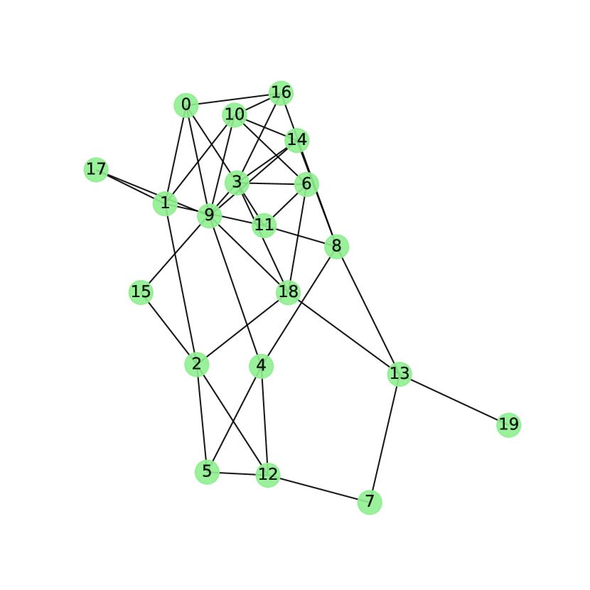
(a) $A=20$, $p_{ER}^{N}=0.2$

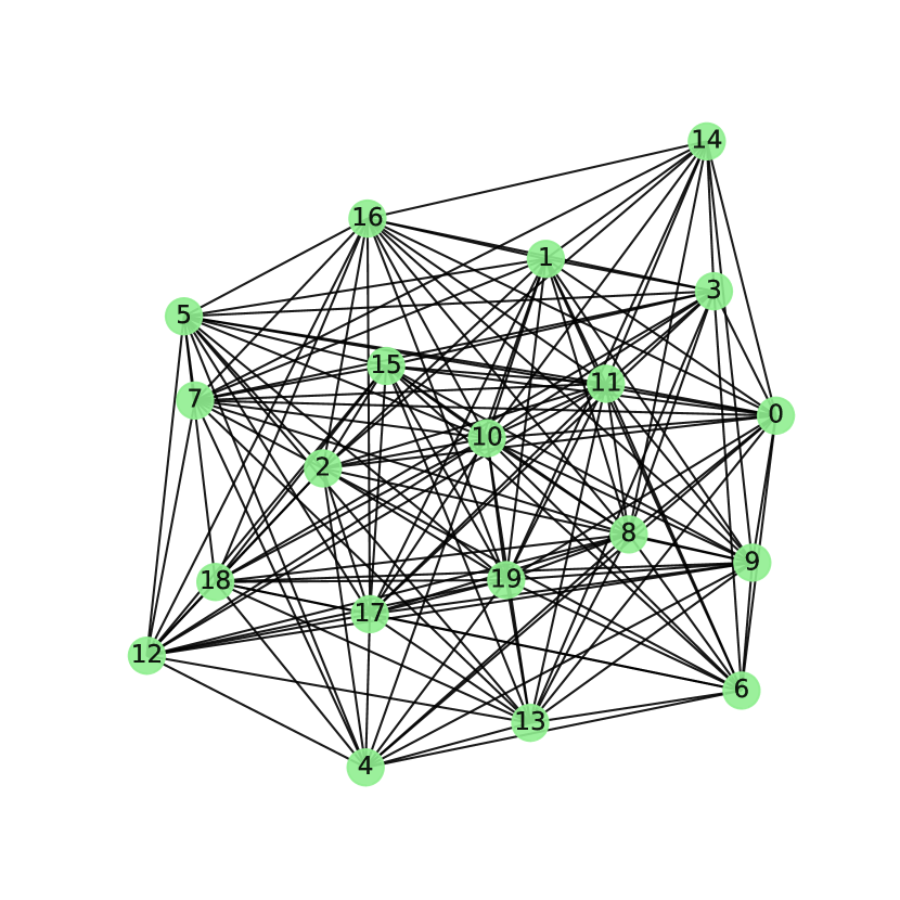
(b) $A=20$, $p_{ER}^{N}=0.8$

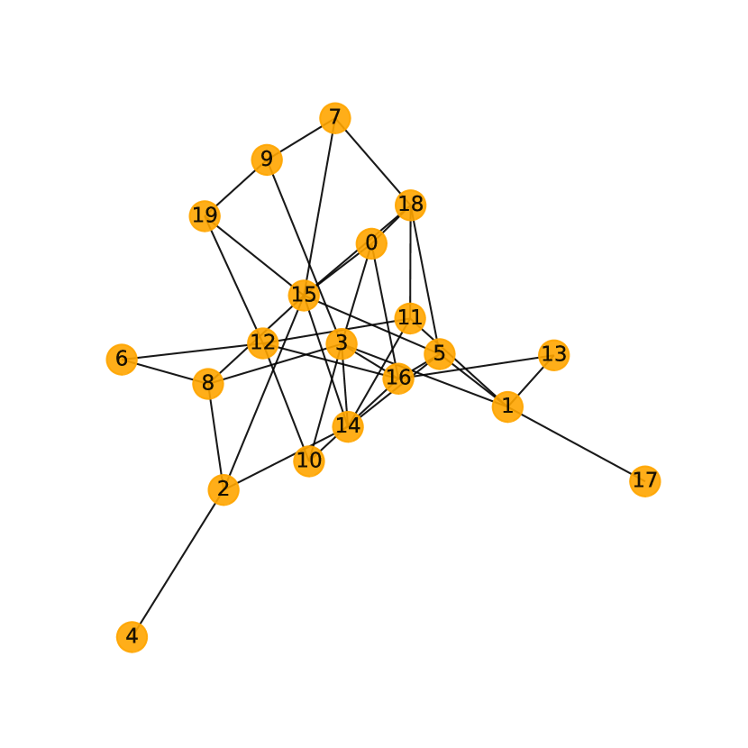
(c) $K=20$, $p_{ER}^{F}=0.2$

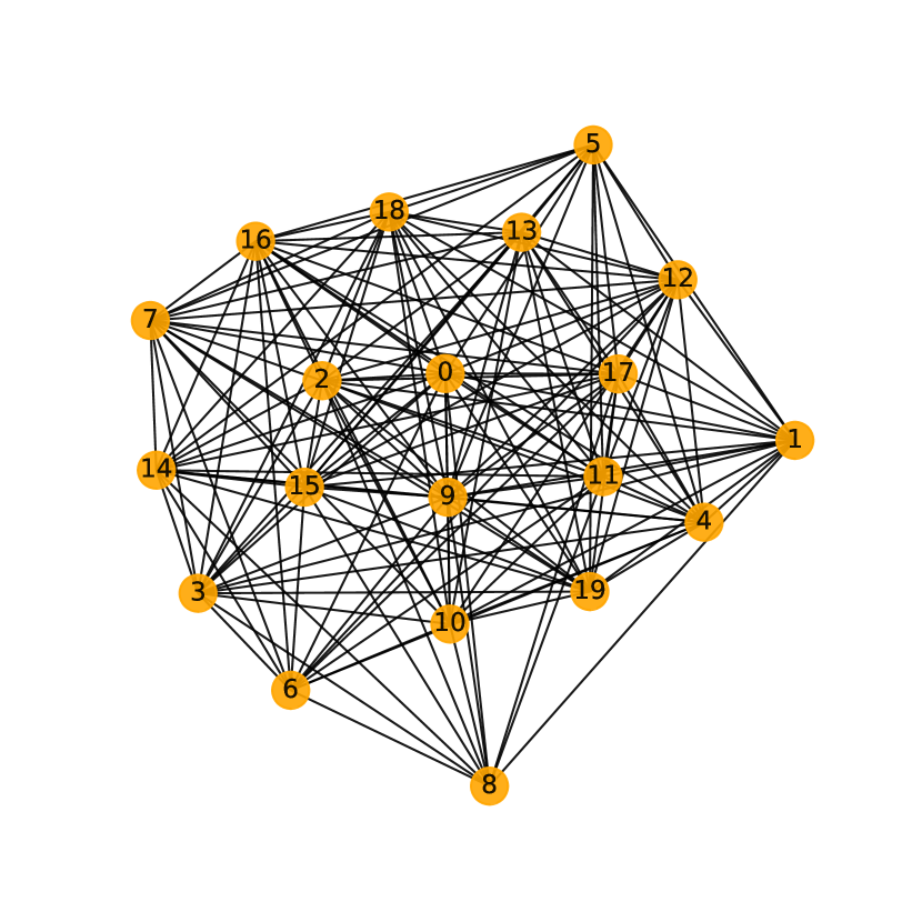
(d) $K=20$, $p_{ER}^{F}=0.8$

Figure 1: The random instances of $N$ (leftmost graphs) and $F$ (rightmost graphs) used in our experiments. The sparse graphs are Erdős–Rényi of parameter $0.2$, the dense graphs are Erdős–Rényi of parameter $0.8$.

In each experiment, Exp3-$\alpha^{2}$ and our baseline are run on the same realization of losses and agent activations. Hence, the only stochasticity left is the internal randomization of the algorithms. Our results are averages of $20$ repetitions of each experiment with respect to this randomization.

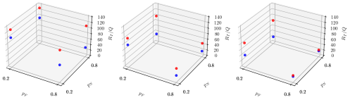
Figure 2: Average regret of Exp3-$\alpha^{2}$ (blue dots) against the baseline (red dots). The $X$-axis and the $Y$-axis correspond to the parameters $p_{F}$ and $p_{N}$ of the Erdős–Rényi graph, the $Z$-axis is the average regret $R_{T}/Q$. The three plots correspond to increasing values (from left to right) of activation probability: $q=0.05$ (leftmost plot), $q=0.5$ (central plot), $q=1$ (rightmost plot).

Figure 2 summarizes the results of our experiments in terms of the average regret $R_{T}/Q$. See Appendix D for the actual learning curves. Recall that our upper bound (1) scales with the quantity $\sqrt{\alpha(N\boxtimes F)/Q}$.

• Note that our algorithm (blue dots) is never worse than the baseline (red dots). This is consistent with the fact that $N$ for the baseline is the edgeless graph, implying that $\alpha(N\boxtimes F)=A\,\alpha(F)$.

• Consistently with (1), the average performance gets worse when $Q\to 1$.

• By construction, the performance of the baseline in each plot remains constant when $p_{N}$ varies in $\{0.2,0.8\}$. On the other hand, our algorithm is worse when $N$ is sparse because $\alpha(N\boxtimes F)$ increases.

• The performance of both algorithms is worse when $F$ is sparse because, once more, $\alpha(N\boxtimes F)$ increases.

6 Conclusions

Previous existing papers considered extreme special cases of our cooperative learning with feedback graphs framework. Cesa-Bianchi et al. [2016] show that in a bandit setting, where all agents are active at all time steps, communication speeds up learning by reducing the variance of loss estimates. On the opposite side of the spectrum, Cesa-Bianchi et al. [2020] prove that updating also non-active agents improve rates in full-information settings. These considerations left open the question of which updates would help in all intermediate settings and why. In this paper, we prove that both types of updates help local learners across the entire experts-bandits spectrum (Theorem 1) and show that no other strategy can perform significantly better in general (Theorem 3). We stress that the success of this strategy crucially depends on the stochasticity of the activations. Indeed, Cesa-Bianchi et al. [2020] disproved the naive intuition that more information automatically translates into better bounds, showing how using all the available data can lead to linear regret in some cases.

Appendix A Further Related Work

The topic of cooperation in online learning gathered a vast amount of attention in recent years, and many variants of the problem have attracted the interest of the community.

Adversarial losses.

A setting closely related to ours is investigated by Herbster et al. [2021]. However, they assume that the learner has full knowledge of the communication network (a weighted undirected graph), and provide bounds for a harder notion of regret defined with respect to an unknown smooth function mapping users to actions. Bar-On and Mansour [2019] bound the individual regret (as opposed to our network regret) in the adversarial bandit setting of Cesa-Bianchi et al. [2016], in which all agents are active at all time steps. Their results, as well as the results of Cesa-Bianchi et al. [2016], have been extended to cooperative linear bandits by Ito et al. [2020]. Della Vecchia and Cesari [2021] study cooperative linear semibandits and focus on computational efficiency. Dubey et al. [2020a] show regret bounds for cooperative contextual bandits, where the reward obtained by an agent is a linear function of the contexts.

Stochastic losses.

Cooperative stochastic bandits are also an important topic in the online learning community. Recently studied variants of cooperative stochastic bandits consider agent-specific restrictions on feedback [Chen et al., 2021] or on access to arms [Yang et al., 2022], bounded communication [Martínez-Rubio et al., 2019], corrupted communication [Madhushani et al., 2021], heavy-tailed reward distributions [Dubey et al., 2020b], stochastic cooperation models [Chawla et al., 2020], strategic agents [Dubey and Pentland, 2020], and Bayesian agents [Lalitha and Goldsmith, 2021].

Appendix B Graph-Theoretic Results

In this section, we present a general version of a graph-theoretic lemma (Lemma 5) that is crucial for our positive results in Sections 3 and 3.1. Before stating it, we recall two known results.

The first result is a direct consequence of Alon et al. [2017, Lemma 10] specialized to undirected graphs.

Lemma 2.

Let $\mathcal{G}=(\mathcal{V},\mathcal{E})$ be an undirected graph containing all self-loops and $\alpha_{d}(\mathcal{G})$ its $d$-th independence number. For all $i\in\mathcal{V}$, let $\mathcal{N}_{d}^{\mathcal{G}}(i)$ be the $d$-th neighborhood of $i$, $p(i)\geq 0$, and $P(i)=\sum_{j\in\mathcal{N}_{d}^{\mathcal{G}}(i)}p(j)>0$. Then

$$\sum_{i\in\mathcal{V}}\frac{p(i)}{P(i)}\leq\alpha_{d}(\mathcal{G})$$

Proof.

Initialize $V_{1}=\mathcal{V}$, fix $j_{1}\in\operatorname*{argmin}_{j\in V_{1}}P(j)$, and denote $V_{2}=\mathcal{V}\setminus\mathcal{N}(j_{1})$. For $k\geq 2$ fix $j_{k}\in\operatorname*{argmin}_{j\in V_{k}}P(j)$ and shrink $V_{k+1}=V_{k}\setminus\mathcal{N}(j_{k})$ until $V_{k+1}=\varnothing$. Since $\mathcal{G}$ is undirected $j_{k}\notin\bigcup_{s=1}^{k-1}\mathcal{N}(j_{s})$, therefore the number $m$ of times that an action can be picked this way is upper bounded by $\alpha$. Denoting $\mathcal{N}^{\prime}(j_{k})=V_{k}\cap\mathcal{N}(j_{k})$ this implies

$$\sum_{i\in\mathcal{V}}\frac{p(i)}{P(i)} =\sum_{k=1}^{m}\sum_{i\in\mathcal{N}^{\prime}(j_{k})}\frac{p(i)}{P(i)}\leq\sum_{k=1}^{m}\sum_{i\in\mathcal{N}^{\prime}(j_{k})}\frac{p(i)}{P(j_{k})}\leq\sum_{k=1}^{m}\frac{\sum_{i\in\mathcal{N}(j_{k})}p(i)}{P(j_{k})}=m\leq\alpha$$

concluding the proof. ∎

The second result is proven in Cesa-Bianchi et al. [2016, Lemma 3], but here we give a slightly different proof based on the AM-GM inequality.

Lemma 3.

Let $\mathcal{G}=(\mathcal{V},\mathcal{E})$ be an undirected graph containing all self-loops and $\alpha_{d}(\mathcal{G})$ its $d$-th independence number. For all $v\in\mathcal{V}$, let $\mathcal{N}_{d}^{\mathcal{G}}(v)$ be the $d$-th neighborhood of $v$, $c(v)\geq 0$, and $C(v)=1-\prod_{w\in\mathcal{N}_{d}^{\mathcal{G}}(v)}\bigl{(}1-c(w)\bigr{)}>0$. Then

$$\sum_{v\in\mathcal{V}}\frac{c(v)}{C(v)}\leq\frac{1}{1-e^{-1}}\left(\alpha_{d}(\mathcal{G})+\sum_{v\in\mathcal{V}}c(v)\right)$$

Proof.

Set for brevity $P(v)=\sum_{w\in\mathcal{N}_{d}^{\mathcal{G}}(v)}c(w)$. Then we can write

$$\sum_{v\in\mathcal{V}}\frac{c(v)}{C(v)} =\underbrace{\sum_{v\in\mathcal{V}\,:\,P(v)\geq 1}\frac{c(v)}{C(v)}}_{\mathrm{(I)}}\quad+\quad\underbrace{\sum_{v\in\mathcal{V}\,:\,P(v)<1}\frac{c(v)}{C(v)}}_{\mathrm{(II)}}$$

and proceed by upper bounding the two terms (I) and (II) separately. Let $r(v)$ be the cardinality of $\mathcal{N}_{d}^{\mathcal{G}}(v)$. We have, for any given $v\in\mathcal{V}$,

$$\min\left\{C(v)\,:\,\sum_{w\in\mathcal{N}(v)}c(w)\geq 1\right\}=\min\left\{C(v)\,:\,\sum_{w\in\mathcal{N}(v)}c(w)=1\right\}$$

$$\qquad=1-\max\left\{\prod_{w\in\mathcal{N}_{d}^{\mathcal{G}}(v)}\bigl{(}1-c(w)\bigr{)}\,:\,\sum_{w\in\mathcal{N}(v)}\bigl{(}1-c(w)\bigr{)}=r(v)-1\right\}$$

$$\qquad\geq 1-\left(1-\frac{1}{r(v)}\right)^{r(v)}\geq 1-e^{-1}$$

where the first equality follows from the definition of $C(v)$ and the monotonicity of $x\mapsto 1-x$, the first inequality is implied by the AM-GM inequality (Lemma 4), and the last one comes from $r(v)\geq 1$ (for $v\in\mathcal{N}_{d}^{\mathcal{G}}(v)$). Hence

$$\mathrm{(I)}\leq\sum_{v\in\mathcal{V}\,:\,P(v)\geq 1}\frac{c(v)}{1-e^{-1}}\leq\sum_{v\in\mathcal{V}}\frac{c(v)}{1-e^{-1}}$$

As for (II), using the inequality $1-x\leq e^{-x}$, $x\in\mathbb{R}$, with $x=c(w)$, we can write

$$C(v)\geq 1-\exp\left(-\sum_{w\in\mathcal{N}_{d}^{\mathcal{G}}(v)}c(w)\right)=1-\exp\left(-P(v)\right)$$

Now, since in (II) we are only summing over $v$ such that $P(v)<1$, we can use the inequality $1-e^{-x}\geq(1-e^{-1})\,x$, holding when $x\in[0,1]$, with $x=P(v)$, thereby concluding that

$$C(v)\geq(1-e^{-1})P(v)$$

Thus

$$\mathrm{(II)}\leq\sum_{v\in\mathcal{V}\,:\,P(v)<1}\frac{c(v)}{(1-e^{-1})P(v)}\leq\frac{1}{1-e^{-1}}\,\sum_{v\in\mathcal{V}}\frac{c(v)}{P(v)}\leq\frac{\alpha}{1-e^{-1}}$$

where in the last step we used Lemma 2. ∎

The following result, known as the inequality of arithmetic and geometric means, or simply AM-GM inequality, is used in the proofs of Lemmas 1, 3, and 5.

Lemma 4 (AM-GM inequality).

For any $x_{1},\dots,x_{r}\in[0,\infty)$,

$$\frac{x_{1}+\dots+x_{r}}{r}\geq(x_{1}\cdot\dots\cdot x_{r})^{1/r}$$

Proof.

By Jensen’s inequality,

$$\ln\left(\frac{1}{r}\sum_{i=1}^{r}x_{i}\right)\geq\sum_{i=1}^{r}\frac{1}{r}\ln\left(x_{i}\right)=\sum_{i=1}^{r}\ln\left(x_{i}^{1/r}\right)=\ln\left(\prod_{i=1}^{r}x_{i}^{1/r}\right)$$

∎

We can now state a more general version of our key graph-theoretic result, which can be proved similarly to Lemma 1.

Lemma 5.

Let $\mathcal{G}_{1}=(\mathcal{V}_{1},\mathcal{E}_{1})$ and $\mathcal{G}_{2}=(\mathcal{V}_{2},\mathcal{E}_{2})$ be two undirected graphs containing all self-loops and $\alpha\big{(}\mathcal{G}_{1}\boxtimes\mathcal{G}_{2}\big{)}$ the independence number of their strong product $\mathcal{G}_{1}\boxtimes\mathcal{G}_{2}$. For all $(i,j)\in\mathcal{V}_{1}\times\mathcal{V}_{2}$, let also $\mathcal{N}_{1}^{\mathcal{G}_{1}}(i)$, $\mathcal{N}_{1}^{\mathcal{G}_{2}}(v)$, and $\mathcal{N}_{1}^{\mathcal{G}_{1}\boxtimes\mathcal{G}_{2}}(i,v)$ be the first neighborhoods of $i$ (in $\mathcal{G}_{1}$), $v$ (in $\mathcal{G}_{2}$), and $(i,v)$ (in $\mathcal{G}_{1}\boxtimes\mathcal{G}_{2}$). If $\boldsymbol{w}=\bigl{(}w(j,u)\bigr{)}_{(j,u)\in\mathcal{V}_{1}\times\mathcal{V}_{2}}$ is an arbitrary matrix with non-negative entries such that $1-\sum_{j\in\mathcal{N}_{1}^{\mathcal{G}_{1}}(i)}w(j,u)\geq 0$ for all $(i,u)\in\mathcal{V}_{1}\times\mathcal{V}_{2}$ and $1-\prod_{u\in\mathcal{N}_{1}^{\mathcal{G}_{2}}(v)}\bigl{(}1-\sum_{j\in\mathcal{N}_{1}^{\mathcal{G}_{1}}(i)}w(j,u)\bigr{)}>0$ for all $(i,v)\in\mathcal{V}_{1}\times\mathcal{V}_{2}$, then

$$\sum_{i\in\mathcal{V}_{1}}\sum_{v\in\mathcal{V}_{2}}\frac{w(i,v)}{1-\prod_{u\in\mathcal{N}_{1}^{\mathcal{G}_{2}}(v)}\bigl{(}1-\sum_{j\in\mathcal{N}_{1}^{\mathcal{G}_{1}}(i)}w(j,u)\bigr{)}}\leq\frac{e}{e-1}\left(\alpha\big{(}\mathcal{G}_{1}\boxtimes\mathcal{G}_{2}\big{)}+\sum_{i\in\mathcal{V}_{1}}\sum_{v\in\mathcal{V}_{2}}w(i,v)\right)$$

We conclude this section by presenting an example where the independence number of the strong product of two graphs significantly differs from the product of their individual independence numbers.

Example 1.

Take as the first graph $G_{1}=(V_{1},E_{1})$, the cycle $C_{5}$ over $5$ vertices. Then, for any $k\geq 2$, build $G_{k}=(V_{k},E_{k})$ inductively by replacing each vertex $v\in V_{k-1}$ by a copy of $C_{5}$ and each edge $e\in E_{k-1}$ by a copy of $K_{5,5}$ (the complete bipartite graph with partitions of size $5$ and $5$) between the two copies of $C_{5}$ that replaced its endpoints. It can be shown that $\alpha(G_{k})=2^{k}$ but $\alpha\big{(}G_{k}\boxtimes G_{k}\big{)}\geq 5^{k}\gg 4^{k}=\alpha_{1}^{G_{k}}\alpha(G_{k})$.

To see why, note first that $\alpha(C_{5})=2$ but $\alpha\big{(}C_{5}\boxtimes C_{5}\big{)}\geq 5$, by choosing the independent set containing the $5$ vertices $(1,1)$, $(2,3)$, $(3,5)$, $(4,2)$, $(5,4)$. For $k\geq 2$, $\alpha(G_{k})=2^{k}$ but we can take the analogous in $G_{k}\boxtimes G_{k}$ of the above independent set in $C_{5}\boxtimes C_{5}$. This gives $5$ sets $S_{1},S_{2},S_{3},S_{4},S_{5}$ of $25^{k-1}$ vertices each, with no edges between $S_{i},S_{j}$ when $i\neq j$. The subgraph of $G_{k}\boxtimes G_{k}$ induced by each $S_{i}$ is simply the previous iteration $G_{k-1}$ of this construction, and proceeding by induction we can find an independent subset of each $S_{i}$ with $5^{k-1}$ vertices, giving a total of $5^{k}$ independent vertices.

Appendix C The upper bound of Cesa-Bianchi et al. [2020] for the expert case

Cesa-Bianchi et al. [2020, Theorem 10] gives theoretical guarantees for the average regret over active agents. In this section, we briefly discuss how to convert their statement to a corresponding result for the total regret over active agents that is the focus of our present work.

Before stating the theorem, we recall that the convex conjugate $f^{*}\colon\mathbb{R}^{d}\to\mathbb{R}$ of a convex function $f\colon\mathbb{X}\to\mathbb{R}$ is defined, for any $\boldsymbol{x}\in\mathbb{R}^{d}$, by $f^{*}(\boldsymbol{x})=\sup_{\boldsymbol{w}\in\mathbb{X}}\big{(}\boldsymbol{x}\cdot\boldsymbol{w}-f(\boldsymbol{w})\big{)}$. Moreover, given $\sigma>0$, we say that $f$ is $\sigma$-strongly convex on $\mathbb{X}$ with respect to a norm $\left\lVert\cdot\right\rVert$ if, for all $\boldsymbol{u},\boldsymbol{w}\in\mathbb{X}$, we have $f(\boldsymbol{u})\geq f(\boldsymbol{w})+\nabla f(\boldsymbol{w})\cdot(\boldsymbol{u}-\boldsymbol{w})+\frac{\sigma}{2}\left\lVert\boldsymbol{u}-\boldsymbol{w}\right\rVert^{2}$. The following well-known result can be found in Shalev-Shwartz et al. [2012, Lemma 2.19 and subsequent paragraph].

Lemma 6.

Let $f\colon\mathbb{X}\to\mathbb{R}$ be a strongly convex function on $\mathbb{X}$. Then the convex conjugate $f^{*}$ is everywhere differentiable on $\mathbb{R}^{d}$.

input: $\sigma_{t}$-strongly convex regularizers $g_{t}\colon\mathbb{X}\to\mathbb{R}$ for $t=1,2,\dots$

initialization: $\boldsymbol{\theta}_{1}=\boldsymbol{0}\in\mathbb{R}^{d}$

for $t=1,2,\dots$  do

     choose $\boldsymbol{w}_{t}=\nabla g_{t}^{*}(\boldsymbol{\theta}_{t})$

      observe $\nabla\ell_{t}(\boldsymbol{w}_{t})\in\mathbb{R}^{d}$

      update $\boldsymbol{\theta}_{t+1}=\boldsymbol{\theta}_{t}-\nabla\ell_{t}(\boldsymbol{w}_{t})$

Algorithm 2

The following result—see, e.g., Orabona et al. [2015, bound (6) in Corollary 1 with $F$ set to zero]—shows an upper bound on the regret of Algorithm 2 for single-agent online convex optimization with expert feedback.

Theorem 4.

Let $g\colon\mathbb{X}\to\mathbb{R}$ be a differentiable function $\sigma$-strongly convex with respect to $\left\lVert\cdot\right\rVert$. Then the regret of Algorithm 2 run with $g_{t}=\frac{\sqrt{t}}{\eta}g$, for $\eta>0$, satisfies

$$\sum_{t=1}^{T}\ell_{t}\big{(}\boldsymbol{x}_{t}\big{)} -\inf_{\boldsymbol{x}\in\mathbb{X}}\sum_{t=1}^{T}\ell_{t}(\boldsymbol{x})\leq\frac{D}{\eta}\sqrt{T}+\frac{\eta}{2\sigma}\sum_{t=1}^{T}\frac{1}{\sqrt{t}}\left\lVert\nabla\ell{}_{t}\right\rVert_{*}^{2}$$

where $D=\sup g$ and $\left\lVert\cdot\right\rVert_{*}$ is the dual norm of $\left\lVert\cdot\right\rVert$. If $\sup\left\lVert\nabla\ell{}_{t}\right\rVert_{*}\leq L$, then choosing $\eta=\sqrt{2\sigma D}/L$ gives $R_{T}\leq L\sqrt{2DT/\sigma}$.

We can now present the equivalent of Cesa-Bianchi et al. [2020, Theorem 10] for cooperative online covenx optimization with expert feedback (i.e., $F$ is a clique) where $n=1$ but the feedback is broadcast to first neighbor immediately after an action is played (rather than the following round).

Theorem 5.

Consider a network $N=(A,E_{N})$ of agents. If all agents $v$ run Algorithm 2 with an oblivious network interface and $g_{t}=\frac{\sqrt{t}}{\eta}g$, where $\left\lVert g_{t}\right\rVert_{*}$ is upper bounded by a constant $L>0$, $\eta>0$ is a learning rate, and the regularizer $g\colon\mathbb{X}\to\mathbb{R}$ is differentiable, $\sigma$-strongly convex with respect to some norm $\left\lVert\cdot\right\rVert$, and upper bounded by a constant $M^{2}$, then the network regret satisfies

$$R_{T}\leq\left(\frac{M^{2}}{\eta}+\frac{\eta L^{2}}{2\sigma}\right)\sqrt{2Q(\alpha(N)+Q)T}$$

For $\eta=\sqrt{2\sigma}M/L$, we have

$$R_{T}\leq\bigl{(}\sqrt{2\sigma}LM\bigr{)}\sqrt{Q(\alpha(N)+Q)T}$$

Proof.

sketch For any $\boldsymbol{x}\in\mathbb{X}$, agent $v$, and time $t$, let $\boldsymbol{x}_{t}(v)$ be the prediction made by $v$ at time $t$, $r_{t}(v,\boldsymbol{x})=\ell_{t}\big{(}\boldsymbol{x}_{t}(v)\big{)}-\ell_{t}(\boldsymbol{x})$, $Q_{v}=\Pr\left(v\in\bigcup_{w\in\mathcal{A}_{t}}\mathcal{N}_{1}^{N}({w})\right)=1-\prod_{w\in\mathcal{N}_{1}^{N}(v)}\big{(}1-q(w)\big{)}$, and $A^{\prime}:=\bigl{\{}w\in A:q(w)>0\bigr{\}}$. Proceeding as in Cesa-Bianchi et al. [2020, Theorem 2] yields, for each $v\in A^{\prime}$ and $\boldsymbol{x}\in\mathbb{X}$,

$$\mathbb{E}\left[\sum_{t=1}^{T}r_{t}(v,\boldsymbol{x})\right]\leq\left(\frac{M^{2}}{\eta}+\frac{\eta L^{2}}{2}\right)\sqrt{\frac{T}{Q_{v}}}$$ (10)

Now, by the independence of the activations of the agents at time $t$ and $\bigl{(}r_{t}(v,\boldsymbol{x})\bigr{)}_{v\in A^{\prime},\boldsymbol{x}\in\mathbb{X}}$, we get

$$R_{T}=\sup_{\boldsymbol{x}\in\mathbb{X}}\sum_{v\in V^{\prime}}q(v)\sum_{t=1}^{T}\mathbb{E}\bigl{[}r_{t}(v,\boldsymbol{x})\bigr{]}$$ (11)

Putting Equations 11 and 10 together and applying Jensen’s inequality yields

$$R_{T}\leq\left(\sum_{v\in V^{\prime}}q(v)\sqrt{\frac{1}{Q_{v}}}\right)\left(\frac{M^{2}}{\eta}+\frac{\eta L^{2}}{2}\right)\sqrt{T}\leq\sqrt{Q\sum_{v\in V^{\prime}}\frac{q_{v}}{Q_{v}}}\left(\frac{M^{2}}{\eta}+\frac{\eta L^{2}}{2}\right)\sqrt{T}$$

The proof is concluded by invoking Lemma 3. ∎

Appendix D Learning curves

Learning curves for the experiments described in Section 5. We plot the average regret $R_{T}/Q$ against the number $T$ of rounds. Our algorithm is the blue curve and the baseline is the red curve. Recall that these curves are averages over $20$ repetitions of the same experiment (the shaded areas correspond to one standard deviation) where the stochasticity is due to the internal randomization of the algorithms.

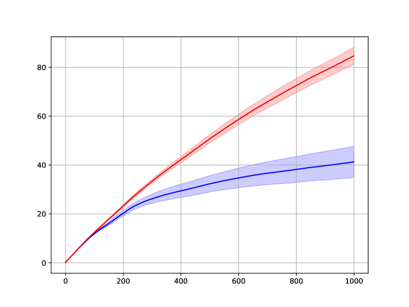
(a) $p_{ER}^{N}=0.2$, $p_{ER}^{F}=0.2$

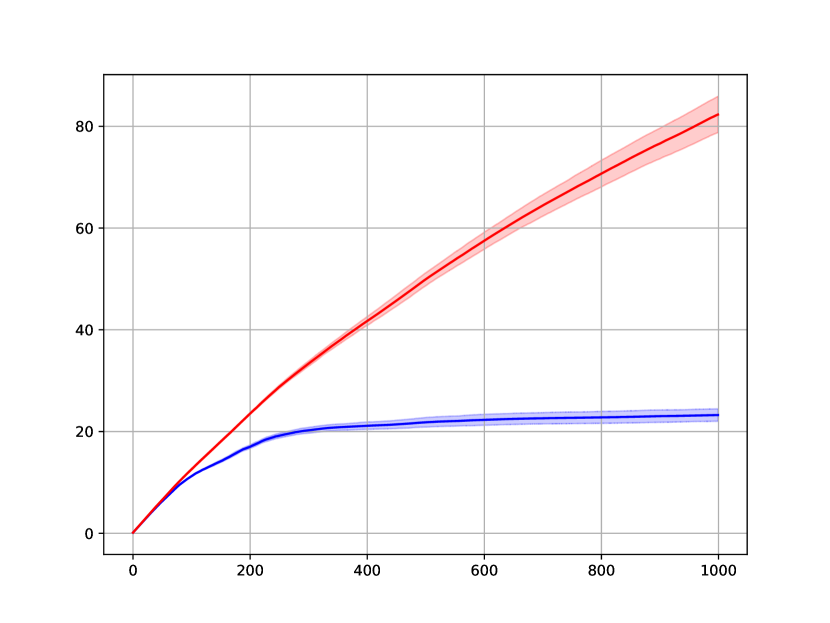
(b) $p_{ER}^{N}=0.8$, $p_{ER}^{F}=0.2$

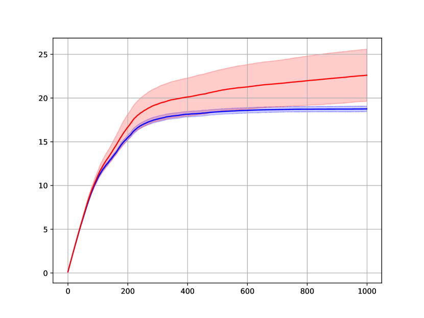
(c) $p_{ER}^{N}=0.2$, $p_{ER}^{F}=0.8$

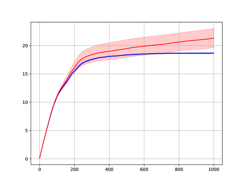
(d) $p_{ER}^{N}=0.8$, $p_{ER}^{F}=0.8$

Figure 3: Activation probability $q=1$.

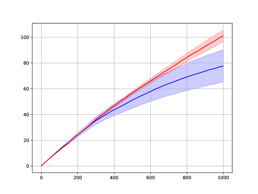
(a) $p_{ER}^{N}=0.2$, $p_{ER}^{F}=0.2$

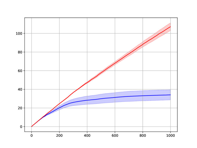
(b) $p_{ER}^{N}=0.8$, $p_{ER}^{F}=0.2$

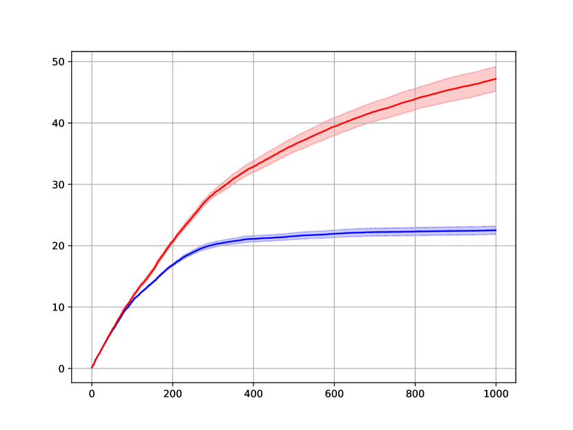
(c) $p_{ER}^{N}=0.2$, $p_{ER}^{F}=0.8$

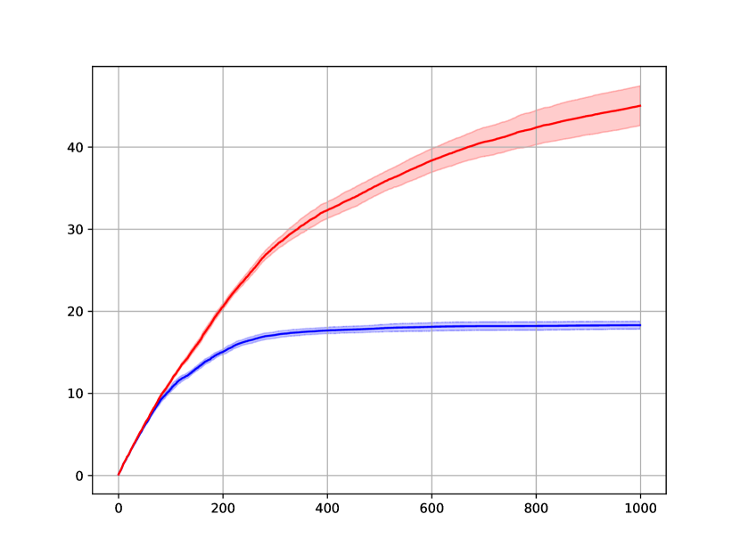
(d) $p_{ER}^{N}=0.8$, $p_{ER}^{F}=0.8$

Figure 4: Activation probability $q=0.5$

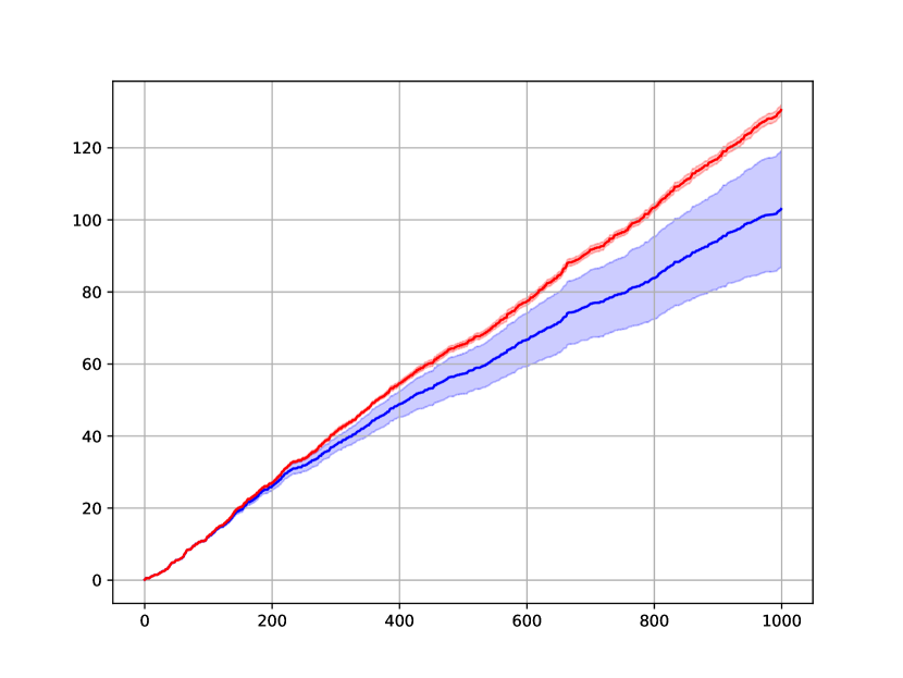
(a) $p_{ER}^{N}=0.2$, $p_{ER}^{F}=0.2$

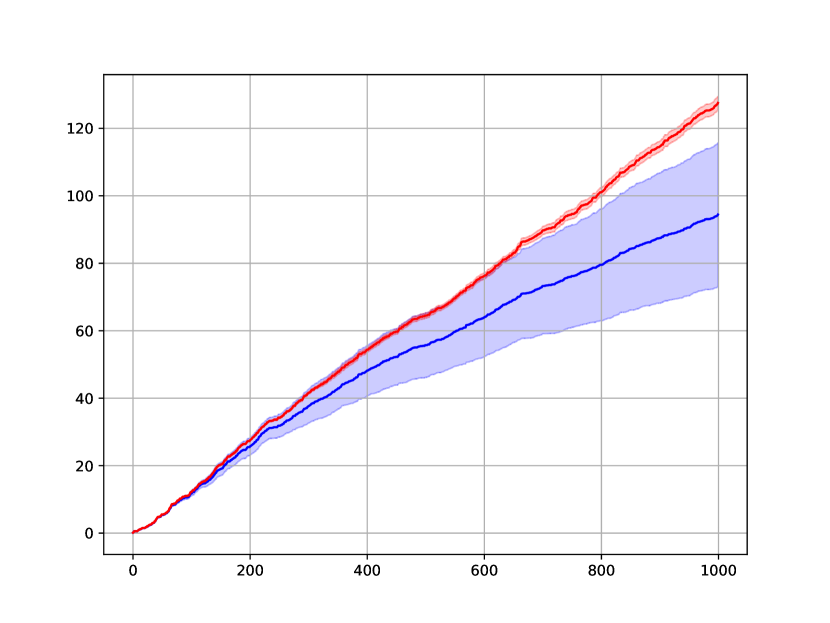
(b) $p_{ER}^{N}=0.8$, $p_{ER}^{F}=0.2$

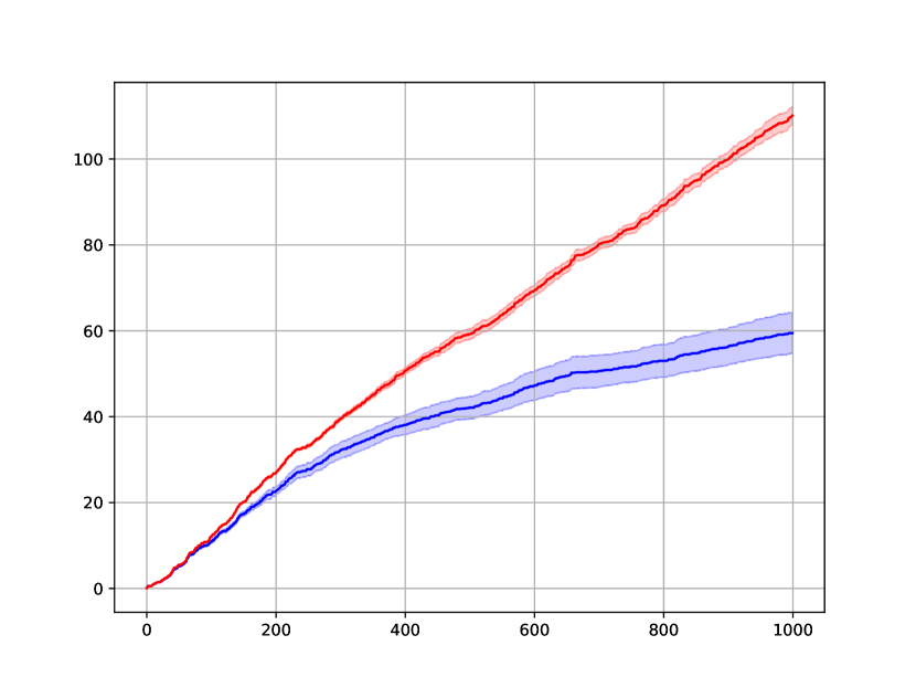
(c) $p_{ER}^{N}=0.2$, $p_{ER}^{F}=0.8$

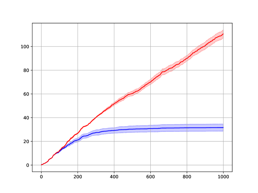
(d) $p_{ER}^{N}=0.8$, $p_{ER}^{F}=0.8$

Figure 5: Activation probability $q=0.05$

References

- Orabona [2019] Francesco Orabona. A modern introduction to online learning. arXiv preprint arXiv:1912.13213, 2019.
- Cesa-Bianchi et al. [2020] Nicolò Cesa-Bianchi, Tommaso Cesari, and Claire Monteleoni. Cooperative online learning: Keeping your neighbors updated. In Algorithmic Learning Theory, pages 234–250. PMLR, 2020.
- Cesa-Bianchi et al. [2016] Nicolò Cesa-Bianchi, Claudio Gentile, Yishay Mansour, and Alberto Minora. Delay and cooperation in nonstochastic bandits. In Conference on Learning Theory, pages 605–622. PMLR, 2016.
- Alon et al. [2017] Noga Alon, Nicolo Cesa-Bianchi, Claudio Gentile, Shie Mannor, Yishay Mansour, and Ohad Shamir. Nonstochastic multi-armed bandits with graph-structured feedback. SIAM Journal on Computing, 46(6):1785–1826, 2017.
- Gyorgy and Joulani [2021] Andras Gyorgy and Pooria Joulani. Adapting to delays and data in adversarial multi-armed bandits. In International Conference on Machine Learning, pages 3988–3997. PMLR, 2021.
- Carpentier and Valko [2016] Alexandra Carpentier and Michal Valko. Revealing graph bandits for maximizing local influence. In Artificial Intelligence and Statistics, pages 10–18. PMLR, 2016.
- Joulani et al. [2020] Pooria Joulani, András György, and Csaba Szepesvári. A modular analysis of adaptive (non-) convex optimization: Optimism, composite objectives, variance reduction, and variational bounds. Theoretical Computer Science, 808:108–138, 2020.
- Hales [1973] R. Stanton Hales. Numerical invariants and the strong product of graphs. Journal of Combinatorial Theory, Series B, 15(2):146–155, 1973.
- Acín et al. [2017] Antonio Acín, Runyao Duan, David E Roberson, Ana Belén Sainz, and Andreas Winter. A new property of the Lovász number and duality relations between graph parameters. Discrete Applied Mathematics, 216:489–501, 2017.
- Rosenfeld [1967] Moshe Rosenfeld. On a problem of C.E. Shannon in graph theory. Proceedings of the American Mathematical Society, 18(2):315–319, 1967.
- Herbster et al. [2021] Mark Herbster, Stephen Pasteris, Fabio Vitale, and Massimiliano Pontil. A gang of adversarial bandits. Advances in Neural Information Processing Systems, 34, 2021.
- Bar-On and Mansour [2019] Yogev Bar-On and Yishay Mansour. Individual regret in cooperative nonstochastic multi-armed bandits. In Advances in Neural Information Processing Systems, volume 32. Curran Associates, Inc., 2019.
- Ito et al. [2020] Shinji Ito, Daisuke Hatano, Hanna Sumita, Kei Takemura, Takuro Fukunaga, Naonori Kakimura, and Ken-Ichi Kawarabayashi. Delay and cooperation in nonstochastic linear bandits. Advances in Neural Information Processing Systems, 33:4872–4883, 2020.
- Della Vecchia and Cesari [2021] Riccardo Della Vecchia and Tommaso Cesari. An efficient algorithm for cooperative semi-bandits. In Algorithmic Learning Theory, pages 529–552. PMLR, 2021.
- Dubey et al. [2020a] Abhimanyu Dubey et al. Kernel methods for cooperative multi-agent contextual bandits. In International Conference on Machine Learning, pages 2740–2750. PMLR, 2020a.
- Chen et al. [2021] Yu-Zhen Janice Chen, Stephen Pasteris, Mohammad Hajiesmaili, John Lui, Don Towsley, et al. Cooperative stochastic bandits with asynchronous agents and constrained feedback. Advances in Neural Information Processing Systems, 34, 2021.
- Yang et al. [2022] Lin Yang, Yu-zhen Janice Chen, Mohammad Hajiesmaili, John Lui, and Don Towsley. Distributed bandits with heterogeneous agents. arXiv preprint arXiv:2201.09353, 2022.
- Martínez-Rubio et al. [2019] David Martínez-Rubio, Varun Kanade, and Patrick Rebeschini. Decentralized cooperative stochastic bandits. Advances in Neural Information Processing Systems, 32, 2019.
- Madhushani et al. [2021] Udari Madhushani, Abhimanyu Dubey, Naomi Leonard, and Alex Pentland. One more step towards reality: Cooperative bandits with imperfect communication. Advances in Neural Information Processing Systems, 34, 2021.
- Dubey et al. [2020b] Abhimanyu Dubey et al. Cooperative multi-agent bandits with heavy tails. In International Conference on Machine Learning, pages 2730–2739. PMLR, 2020b.
- Chawla et al. [2020] Ronshee Chawla, Abishek Sankararaman, Ayalvadi Ganesh, and Sanjay Shakkottai. The gossiping insert-eliminate algorithm for multi-agent bandits. In International Conference on Artificial Intelligence and Statistics, pages 3471–3481. PMLR, 2020.
- Dubey and Pentland [2020] Abhimanyu Dubey and Alex Pentland. Private and byzantine-proof cooperative decision-making. In AAMAS, pages 357–365, 2020.
- Lalitha and Goldsmith [2021] Anusha Lalitha and Andrea Goldsmith. Bayesian algorithms for decentralized stochastic bandits. IEEE Journal on Selected Areas in Information Theory, 2(2):564–583, 2021.
- Shalev-Shwartz et al. [2012] Shai Shalev-Shwartz et al. Online learning and online convex optimization. Foundations and trends in Machine Learning, 4(2):107–194, 2012.
- Orabona et al. [2015] Francesco Orabona, Koby Crammer, and Nicolò Cesa-Bianchi. A generalized online mirror descent with applications to classification and regression. Machine Learning, 99(3):411–435, 2015.