Electric field induced injection and shift currents in zigzag graphene nanoribbons

Abstract

We theoretically investigate the one-color injection currents and shift currents in zigzag graphene nanoribbons with applying a static electric field across the ribbon, which breaks the inversion symmetry to generate nonzero second order optical responses by dipole interaction. These two types of currents can be separately excited by specific light polarization, circularly polarized lights for injection currents and linearly polarized lights for shift currents. Based on a tight binding model formed by carbon 2p_z orbitals, we numerically calculate the spectra of injection coefficients and shift conductivities, as well as their dependence on the static field strength and ribbon width. The spectra show many peaks associated with the optical transition between different subbands, and the positions and amplitudes of these peaks can be effectively controlled by the static electric field. By constructing a simple two band model, the static electric fields are found to modify the edge states in a nonperturbative way, and their associated optical transitions dominate the current generation at low photon energies. For typical parameters, such as a static field 10⁶ V/m and light intensity 0.1 GW/cm², the magnitude of the injection and shift currents for a ribbon with width 5 nm can be as large as the order of 1 $\mu$A. Our results provide a physical basis for realizing passive optoelectronic devices based on graphene nanoribbons.

I Introduction

Graphene nanoribbon (GNR) is a narrow stripe of monolayer graphene with width varying from a few nanometers to less than 50 nanometers, at which it shows exciting physical properties in addition to graphene due to the quantum confinement.PhysRevLett.97.216803 Combining with its compatibility with industry-standard lithographic processing Nat.Mater._8_235_2009_Ritter ; J.Phys.Chem.B_108_19912_2004_Berger and the increasingly mature fabrication procedure ActaPhysicaSinica_68_168102_2019_Chen , GNR is considered as a potential material for applications in nanoelectronics and optoelectronics. Many efforts have been devoted to understand its band structures, transport properties, magnetism, chirality, optical properties, and so on grapheneoptoelectronic1 ; graphenetransport ; NaturePhys_7_616_Chenggang_Tao ; PhysRevB.59.8271 .

The widely studied GNRs include armchair GNRs (aGNRs) with edges orientated along the armchair directions and zigzag GNRs (zGNRs) with edges orientated along the zigzag directions. The band structures of GNRs have been calculated by different models, such as tight binding modelPhysRevB.54.17954 , continuum model based on a $\bm{k}\cdot\bm{p}$ HamiltonianPhysRevB.73.235411 , and first principle calculationsPhysRevLett.97.216803 . The simplest tight binding model shows that zGNR is always metallic with flat bands induced by edge states, and aGNR can be either semiconducting or metallic depending on its width PhysRevB.54.17954 . After considering the Coulomb interaction, DFT calculations show that all narrow GNRs have finite gaps, and zGNRs possess antiferromagnetic ground states PhysRevB.77.073412 . The band gap has a strong dependence on the edge orientation and ribbon width. In such tight binding model, both the eigenstates and selection rules of the optical transition can be analytically obtained, and many absorption peaks are induced by the optical transitions between different subbandsPhysRevB.76.045418 ; PhysRevB.95.155438 . The linear optical response shows strong anisotropy along zigzag and armchair directions. With applying an external static electric field across the ribbon, the gap can be effectively tuned and becomes closed at an appropriate field strength; and furthermore the optical properties are effectively modulatedCarbon_44_508_Chang ; JPCM_27_145305_Saroka . Because of the insufficient Coulomb screening, the excitonic effects are important for narrow ribbonsPhysRevLett.101.186401 ; PhysRevB.88.165425 ; AZNRexciton ; PhysRevB.99.165415 .

In addition to linear optical responses, the nonlinear optical properties of GNR also attracted much attention. By tuning the doping level electrically, Cox et al. studied the plasmon-assisted harmonic generation, sum and difference frequency generation, and four-wave mixing of graphene nanostructures Nat.Comm._5_5725_2014_Cox ; Phys.Rev.B_96_045442_2017_Cox , and these calculated responses can be several order of magnitude larger than that of metal nanoparticles with similar sizes. Karimi et al. Phys.Rev.B_97_245403_2018_Karimi investigated the Kerr nonlinearity and third harmonic generation of GNR modulated by scatterings. Attaccalite et al.Phys.Rev.B_95_125403_2017_Attaccalite showed the importance of excitonic effects in the third harmonic generation. Wang and Andersen studied the third harmonic generation of aGNR in the Terahertz frequencies J.Phys.DAppl.Phys._49_1_2016_Wang ; J.Phys.Condens.Matter_28_475301_2016_Wang ; Phys.Rev.B_93_235430_2016_Wang . Salazar et al. Phys.Rev.B_93_075442_2016_Salazar studied two color coherent control of zGNR, and found that the edge states play an important role for low photon energies. Recently, Wu et al. indicated the importance of the edge states in high-order harmonic generation of zGNR Chin.Opt.Lett._18_103201_2020_Wu . Bonabi and Pedersen Phys.Rev.B_99_045413_2019_Bonabi studied the electric field induced second harmonic generation of aGNR.

In this paper, we theoretically study the one-color optical injection current and shift current of zGNR, which are direct currents generated by light with only one single frequency; they are also widely referred as circularly photogalvanic effects and linear photogalvanic effects. These effects are recently well studied in layered materials including BiFeO₃ BIO and monolayer Ge and Sn monochalcogenides PhysRevLett.119.067402 . Because zGNR possesses the inversion symmetry, its second order optical responses are forbidden in the dipole approximation. An external static electric field, which will be refered as a gate field afterwards, is applied to break the inversion symmetry. We discuss the dependence of the response coefficients on the gate field strength and the ribbon width. Our results could be useful for the optoelectronic devices utilizing photogalvanic effects of GNR.

We arrange the paper as follows. In Section II we introduce a tight binding model of zGNR with applying a static electric field, and give the expressions for injection coefficients and shift conductivities. In Section III we discuss the contributions from the edge bands by a simple non-perturbative treatment. In Section IV we discuss the effect of the ribbon width on these coefficients. We conclude in Section V.

II Models

II.1 Tight-Binding model for electronic states

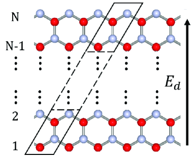
Figure 1: Illustration of a N-zGNR. Red and gray dots correspond to carbon atoms at the A and B sites, respectively. The unit cell of the ribbon is indicated by the parallelogram. An external static electric field $E_{d}$ is applied across the ribbon.

A zGNR with N zigzag lines (N-zGNR) is illustrated in Fig. 1. Taking the $x$ axis along the zigzag direction and the $y$ axis along the perpendicular armchair direction with origin in the center of the ribbon, the carbon atoms locate at ${\bm{R}}_{nm\alpha}=n{\bm{a}}+(m-1){\bm{a}}_{2}+{\bm{\tau}}_{\alpha}-\hat{\bm{y}}W/2$, where ${\bm{a}}=a_{0}\hat{\bm{x}}$ is the primitive lattice vector with the lattice constant ${a}_{0}=2.46$ Å, ${\bm{a}}_{2}=a_{0}(\hat{\bm{x}}+\sqrt{3}\hat{\bm{y}})/2$ and $m=1,2,...,N$ labelling zigzag lines, and ${\bm{\tau}}_{\alpha}$ with $\alpha=A,B$ gives different atom sites as ${\bm{\tau}}_{A}=0$ and ${\bm{\tau}}_{B}=({\bm{a}}_{1}+{\bm{a}}_{2})/3$. The width of a N-zGNR is $W=(N-2/3)\sqrt{3}a_{0}/2$ by taking as the distance between the outermost A and B atom lines. We describe the electronic states in a tight-binding model formed by carbon $2p_{z}$ orbitals with considering the nearest neighbor coupling only. When a gate field $E_{d}$ is applied, the unperturbed Hamiltonian can be written as

$$\hat{H}_{0}=\hat{H}_{h}-eE_{d}\hat{y}$$ (1)

with the electron charge $e=-|e|$. The first term $\hat{H}_{h}$ is a hopping term with matrix elements

$${}_{t}\left\langle n_{1}m_{1}A\right|\hat{H}_{h}\left|n_{2}m_{2}B\right\rangle_{t} ={{}_{t}\left\langle n_{1}m_{1}A\right|\hat{H}_{h}\left|n_{2}m_{2}B\right\rangle_{t}}^{*}$$

$$=-\gamma_{0}(\delta_{n_{1},n_{2}}\delta_{m_{1},m_{2}}+\delta_{n_{1},n_{2}}\delta_{m_{1},m_{2}+1}+\delta_{n_{1}+1,n_{2}}\delta_{m_{1},m_{2}})\,,$$ (2)

$${}_{t}\left\langle n_{1}m_{1}\alpha\right|\hat{H}_{h}\left|n_{2}m_{2}\alpha\right\rangle_{t} =0\,,$$ (3)

where $\gamma_{0}=2.7\,$eV is a hopping parameter between nearest neighbours, the ket $|nm\alpha\rangle_{t}$ stands for the electronic state of the $2p_{z}$ orbital of the carbon atom located at ${\bm{R}}_{nm\alpha}$. The second term is the electrostatic potential, $\hat{y}$ is the $y$-component of the position operator $\hat{\bm{r}}$. In this model, the in-plane position operator has nonzero matrix elements only at the same site as

$${}_{t}\left\langle n_{1}m_{1}\alpha_{1}\right|\hat{\bm{r}}\left|n_{2}m_{2}\alpha_{2}\right\rangle_{t}={\bm{R}}_{n_{1}m_{1}\alpha_{1}}\delta_{n_{1}n_{2}}\delta_{m_{1}m_{2}}\delta_{\alpha_{1}\alpha_{2}}\,.$$ (4)

In Bloch states basis formed by

$$\left|m\alpha,k\right\rangle_{b}=\sqrt{\frac{a_{0}}{2\pi}}\sum_{n}e^{ina_{0}k}\left|nm\alpha\right\rangle_{t}\,,\text{for }0\leq k<g\,,$$ (5)

with $g={2\pi}/{a_{0}}$ being the width of the Brillouin zone, the matrix elements of the Hamiltonian $\hat{H}_{0}$, position operator $\hat{\bm{r}}$, and velocity operator $\hat{\bm{v}}=[\hat{\bm{r}},\hat{H}_{0}]/(i\hbar)$ become

$${}_{b}\langle m_{1}\alpha_{1},k_{1}|\hat{H}_{0}|m_{2}\alpha_{2},k_{2}\rangle_{b} =\tilde{H}^{0}_{m_{1}\alpha_{1},m_{2}\alpha_{2};k}\delta(k_{1}-k_{2})\,,$$ (6)

$${}_{b}\langle m_{1}\alpha_{1},k_{1}|\hat{\bm{r}}|m_{2}\alpha_{2},k_{2}\rangle_{b} =\left[\tilde{\bm{r}}_{m_{1}\alpha_{1},m_{2}\alpha_{2};k_{1}}+i\hat{\bm{x}}\frac{\partial}{\partial k_{1}}\right]\delta(k_{1}-k_{2})\,,$$ (7)

$${}_{b}\langle m_{1}\alpha_{1},k_{1}|\hat{\bm{v}}|m_{2}\alpha_{2},k_{2}\rangle_{b} =\tilde{\bm{v}}_{m_{1}\alpha_{1},m_{2}\alpha_{2};k}\delta(k_{1}-k_{2})\,.$$ (8)

The quantities $\tilde{P}_{m_{1}\alpha_{1},m_{2}\alpha_{2};k}=\sum_{n}e^{ina_{0}k}{{}_{t}\langle}nm_{1}\alpha_{1}|\hat{P}|0m_{2}\alpha_{2}\rangle_{t}$ for $P=H^{0}$, $\bm{r}$ and $\bm{v}$ are the Fourier transform of their matrix elements in the tight binding orbitals, and their matrix elements are

$$\tilde{H}^{0}_{m_{1}A,m_{2}B;k} \equiv[\tilde{H}^{0}_{m_{2}B,m_{1}A;k}]^{\ast}=\gamma_{0}(1+e^{ika_{0}})\delta_{m_{1}m_{2}}+\gamma_{0}\delta_{m_{1}+1,m_{2}}\,,$$ (9)

$$\tilde{H}^{0}_{m_{1}\alpha,m_{2}\alpha;k} =-eE_{d}\tilde{r}^{y}_{m_{1}\alpha,m_{2}\alpha;k}\,,$$ (10)

and

$$\tilde{\bm{r}}_{m_{1}\alpha_{1},m_{2}\alpha_{2};k} =\delta_{m_{1}m_{2}}\delta_{\alpha_{1}\alpha_{2}}\bm{R}_{0m_{1}\alpha_{1}}\,,$$ (11)

$$\tilde{\bm{v}}_{m_{1}\alpha_{1},m_{2}\alpha_{2};k} =\frac{1}{i\hbar}[\tilde{\bm{r}}_{k},\tilde{H}^{0}_{k}]_{m_{1}\alpha_{1},m_{2}\alpha_{2}}+\hat{\bm{x}}\frac{1}{\hbar}\frac{\partial}{\partial k}\tilde{H}^{0}_{m_{1}\alpha_{1},m_{2}\alpha_{2};k}\,.$$ (12)

In the last equation $\tilde{\bm{r}}_{k}$ and $\tilde{H}^{0}_{k}$ are treated as matrices with indexes $m\alpha$. The gate field modifies the on-site energy of each atom.

The band eigenstates $|sk\rangle$ with band index $s$ can be written as

$$|sk\rangle=\sum_{m\alpha}[C_{sk}]_{m\alpha}|m\alpha,k\rangle_{b}\,.$$ (13)

where the coefficients $C_{sk}$ are column eigenvectors satisfying

$$\tilde{H}^{0}_{k}C_{sk}=\varepsilon_{sk}C_{sk}\,,$$ (14)

with the corresponding eigen energy $\varepsilon_{sk}$.

For optical response, the most important quantity is the Berry connection $\bm{\xi}_{s_{1}s_{2}k}$ between band eigenstates, which is defined as

$$\bm{\xi}_{s_{1}s_{2}k} =C^{{\dagger}}_{s_{1}k}\left(\tilde{\bm{r}}_{k}+i\hat{\bm{x}}\frac{\partial}{\partial k}\right)C_{s_{2}k}\,.$$ (15)

The term $\xi^{y}_{s_{1}s_{2}k}$ can be evaluated directly. However, due to the derivative with respect to $k$, the values of $\xi^{x}_{s_{1}s_{2}k}$ depend on the phase of the eigen vectors $C_{sk}$ and is not easy to be evaluated directly. Usually the off-digonal terms can be evaluated from the matrix elements of velocity operator

$$\bm{v}_{s_{1}s_{2}k}=C_{s_{1}k}^{\dagger}\tilde{\bm{v}}_{k}C_{s_{2}k}\,.$$ (16)

The usually used quantities are $\bm{r}_{\bm{k}}$, which are defined as

$$r_{s_{1}s_{2}k}^{y} =\xi_{s_{1}s_{2}k}^{y}\,,\text{ for all }s_{1},s_{2}\,,$$ (17)

$$r_{s_{1}s_{2}k}^{x} \equiv\begin{cases}\xi^{x}_{s_{1}s_{2}k}=\frac{v^{x}_{s_{1}s_{2}k}}{i\omega_{s_{1}s_{2}k}}&\text{ for }s_{1}\neq s_{2}\,,\\ 0&\text{ for }s_{1}=s_{2}\end{cases}$$ (18)

with $\hbar\omega_{s_{1}s_{2}k}=\varepsilon_{s_{1}k}-\varepsilon_{s_{2}k}$. The digonal term of $\xi_{ssk}^{x}$ appears in terms

$${\cal R}_{s_{1}s_{2}k}^{cx}=\frac{\partial}{\partial k}r_{s_{1}s_{2}k}^{c}-i(\xi_{s_{1}s_{1}k}^{x}-\xi_{s_{2}s_{2}k}^{x})r_{s_{1}s_{2}k}^{c}\,,\text{ for }s_{1}\neq s_{2}\,.$$ (19)

with the Roman letter $c$ in the superscript standing for the Cartesian directions $x$ or $y$. A direct calculation gives

$${\cal R}_{s_{1}s_{2}k}^{cx} =-\frac{\Delta_{s_{1}s_{2}k}^{x}r_{s_{1}s_{2}k}^{c}}{\omega_{s_{1}s_{2}k}}+\frac{i[r_{k}^{x},v_{k}^{c}]_{s_{1}s_{2}}+M_{s_{1}s_{2}k}^{cx}}{i\omega_{s_{1}s_{2}k}}\,,$$ (20)

with $\Delta_{s_{1}s_{2}k}^{b}=v_{s_{1}s_{1}k}^{b}-v_{s_{2}s_{2}k}^{b}$ and

$$M_{s_{1}s_{2}k}^{cx} =C_{s_{1}k}^{\dagger}\left(\frac{\partial}{\partial k}\tilde{v}_{k}^{c}-i[\tilde{r}^{x}_{k},\tilde{v}_{k}^{c}]\right)C_{s_{2}k}\,.$$ (21)

For zGNR, ${\cal R}^{yx}_{s_{1}s_{2}k}=i[r_{k}^{x},r_{k}^{y}]_{s_{1}s_{2}}$.

For very narrow zGNR with $N<30$, the interaction between carriers at both edges plays an important role to form antiferromagnetic order, for which the spin orientations are opposite for different edges. For wide ribbons $N>30$, the ferromagnetic-antiferromagnetic energy differences per unit cell are reduced below the order of 1 meVPhysRevLett.97.216803 , hence the magnetic order can be ignored.

II.2 Injection currents and shift currents

In this work, we are interested in the shift current and one-color injection current, both of which arise from the second order optical response. For an incident electric field $\bm{E}(t)=\bm{E}_{0}(t)e^{-i\omega t}+c.c.$ with the slow varying envelope function $\bm{E}_{0}(t)$, the response current includes a (quasi) dc current component $\bm{J}_{0}(t)=J_{0}(t)\hat{\bm{x}}$, which is along the ribbon extension direction only because a dc current cannot flow along the confined dimension. This current approximately includes two parts $J_{0}(t)=J_{i}(t)+J_{s}(t)$. The first term $J_{i}(t)$ is a one-color injection current, and it is

$$\frac{d}{dt}J_{i}(t)=2i\eta^{xbc}(\omega)E_{0}^{b}(t)\left[E_{0}^{c}(t)\right]^{\ast}\,,$$ (22)

and the effective sheet injection rate is $\eta^{xbc}(\omega)=\sum_{s_{1}s_{2}}\eta^{xbc}_{s_{1}s_{2}}(\omega)$ with

$$\eta_{s_{1}s_{2}}^{xbc}(\omega) =-\frac{i\pi e^{3}}{W\hbar^{2}}\int\frac{dk}{2\pi}\Delta^{x}_{s_{1}s_{2}k}\left(r^{c}_{s_{2}s_{1}k}r^{b}_{s_{1}s_{2}k}-r^{b}_{s_{2}s_{1}k}r^{c}_{s_{1}s_{2}k}\right)f_{s_{2}s_{1}k}\delta\left(\omega_{s_{1}s_{2}k}-\omega\right)\,.$$ (23)

Here $f_{s_{2}s_{1}k}=f_{s_{2}k}-f_{s_{1}k}$ gives the population difference in two states $|s_{2}k\rangle$ and $|s_{1}k\rangle$, and $f_{sk}=[1-e^{(\varepsilon_{sk}-\mu)/k_{B}T}]^{-1}$ is Fermi-Dirac distribution for chemical potential $\mu$ and temperature $T$. The spin degeneracy has been included in Eq. (23). The second term $J_{s}(t)$ is a shift current, and it is

$$J_{s}(t) =2\sigma^{xbc}(\omega)E_{0}^{b}(t)\left[E_{0}^{c}(t)\right]^{\ast}\,,$$ (24)

where the effective sheet shift conductivity is $\sigma^{xbc}(\omega)=\sum_{s_{1}s_{2}}\sigma_{s_{1}s_{2}}^{xbc}(\omega)$ with

$$\sigma_{s_{1}s_{2}}^{xbc}(\omega) =-\frac{i\pi e^{3}}{W\hbar^{2}}\int\frac{dk}{2\pi}f_{s_{2}s_{1}k}\left(r^{b}_{s_{1}s_{2}k}{\cal R}^{cx}_{s_{2}s_{1}k}+r^{c}_{s_{1}s_{2}k}{\cal R}^{bx}_{s_{2}s_{1}k}\right)\delta(\omega_{s_{1}s_{2}k}-\omega)\,.$$ (25)

Here we briefly discuss the general properties of $\eta^{xbc}(\omega)$ and $\sigma^{xbc}(\omega)$ from the symmetry argument. The response coefficients of $\eta^{xbc}(\omega)$ and $\sigma^{xbc}(\omega)$ are third order tensors. As a static electric field is applied along the $y$-direction, a zGNR possesses a symmetry $x\leftrightarrow-x$ and the time reversal symmetry. We list the results for $A^{xbc}$ ($A\to\eta$ or $\sigma_{s}$) under each symmetry operation: (1) The symmetry $x\leftrightarrow-x$ determines that the nonzero components are $A^{xxy}$ and $A^{xyx}$. (2) A direct observation of Eqs. (23) and (25) gives $\eta^{xbc}(\omega)=-\eta^{xcb}(\omega)$ and $\sigma_{s}^{xbc}(\omega)=\sigma_{s}^{xcb}(\omega)$. (3) The time reversal symmetryPRB_61_5337_Sipe gives $\bm{r}_{s_{1}s_{2}k}=\bm{r}_{s_{2}s_{1}(-k)}=[\bm{r}_{s_{1}s_{2}(-k)}]^{\ast}$, $\bm{v}_{s_{1}s_{2}k}=-\bm{v}_{s_{2}s_{1}(-k)}=-[\bm{v}_{s_{1}s_{2}(-k)}]^{\ast}$, and $\varepsilon_{sk}=\varepsilon_{s(-k)}$. Furthermore, we can derive $\Delta^{a}_{s_{1}s_{2}k}=-[\Delta_{s_{1}s_{2}(-k)}^{a}]^{\ast}$ and ${\cal R}^{cx}_{s_{1}s_{2}k}=-{\cal R}^{cx}_{s_{2}s_{1}(-k)}=-[{\cal R}^{cx}_{s_{1}s_{2}(-k)}]^{\ast}$. Then we get $\eta^{xbc}(\omega)=[\eta^{xbc}(\omega)]^{\ast}$ from Eq. (23) and $\sigma^{xbc}(\omega)=[\sigma^{xbc}(\omega)]^{\ast}$ from Eq. (25). Using the operations (1)-(3) we find the nonzero components $\eta^{xxy}(\omega)=-\eta^{xyx}(\omega)$ and $\sigma_{s}^{xxy}(\omega)=\sigma_{s}^{xyx}(\omega)$ are real numbers.

Explicitly, by taking the light fields as $\bm{E}_{0}(t)=E_{0}(t)\begin{pmatrix}\cos\theta\\ e^{i\phi}\sin\theta\end{pmatrix}$, the injection and shift currents can be written as

$$\frac{d}{dt}J_{i}(t) =4\eta^{xxy}(\omega)[E_{0}(t)]^{2}\cos\theta\sin\theta\sin\phi\,,$$ (26)

$$J_{s}(t) =4\sigma^{xxy}(\omega)[E_{0}(t)]^{2}\cos\theta\sin\theta\cos\phi\,.$$ (27)

Here $\theta$ and $\phi$ are the polarization orientation angles with respect to the direction $\hat{\bm{x}}$ and the circularity, respectively. Therefore, the appearance of these currents requires both the $x$ and $y$ components of the electric field. The circularly polarized light ($\phi=\pi/2$) generates injection currents only, while the linearly polarized light ($\phi=0$) generates shift currents only.

III Result and Discussions

III.1 Band structure

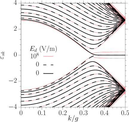
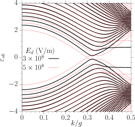
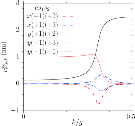
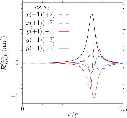
Figure 2: (a,b) Band structures of 24-zGNR for gate field $E_{d}=0$, $10^{8}$ V/m, $3\times 10^{8}$ V/m, and $5\times 10^{8}$ V/m. At zero field, the dashed and solid curves correspond to different parity. The matrix elements of (c) $r^{0;c}_{s_{1}s_{2}k}$ and (d) ${\cal R}^{0;cx}_{s_{1}s_{2}k}$ at zero gate field, with solid (dashed) curves for imaginary (real) parts.

We illustrate the band structures of a 24-zGNR ($W\approx 5$ nm) for different gate field $E_{d}$ in Fig. 2 (a,b). The bands with energies higher than zero are labelled by $s=+1,+2,\cdots$ successively from low energy band to high energy band, and those with energy lower than zero are labelled by $s=-1,-2,\cdots$ in a mirror way. From the symmetry $x\to-x$, the band energies satisfy $\varepsilon_{sk}=\varepsilon_{s(g-k)}$ and $\varepsilon_{sk}=-\varepsilon_{(-s)k}$, and thus they are shown only in half of Brillouin zone. The band structure at zero gate field is plotted in Fig. 2 (a) as black solid and dashed curves. Two bands $s=\pm 1$ are almost flat in the middle of the Brilluion zone, indicating the edge states. The energy difference $\varepsilon_{(+1)k}-\varepsilon_{(-1)k}$ decreases as $k$ approaching $g/2$ and becomes less than 1 meV for $0.38g<k<0.62g$. At $k=g/2$, the two states are strictly degenerate. All other electronic states are confined states. At $k=g/2$, all the state $|sg/2\rangle$ for $s>1$ are degenerate at energy $\gamma_{0}$, and all states $|sg/2\rangle$ for $s<-1$ are degenerate at energy $-\gamma_{0}$. At zero gate field, the inversion symmetry is preserved, and the parity is a good quantum number for each band as $\zeta_{s}=(-1)^{s+1}\text{sgn}[s]$ PhysRevB.95.155438 ; Phys.Rev.B_93_075442_2016_Salazar , which is shown in dashed and solid curves in Fig. 2 (a). There exist selection rules for the velocity matrix elements as $v^{x}_{s_{1}s_{2}k}=0$ for $\zeta_{s_{1}}\neq\zeta_{s_{2}}$ and $v^{y}_{s_{1}s_{2}k}=0$ for $\zeta_{s_{1}}=\zeta_{s_{2}}$, and the same selection rules hold for $\bm{\xi}_{s_{1}s_{2}k}$. Therefore, the nonzero $\xi^{y}_{s_{1}s_{2}k}$ between bands with different parities indicates that the gate field can couple bands with different parities and then the band parity is no longer a good quantum number.

Figure 2 (c) gives the $k$-dependence of $r^{0;c}_{s_{1}s_{2}k}$ for different sets of $cs_{1}s_{2}$, where a quantity at zero gate field is indicated by a superscript “0”. With choosing the wave functions appropriately, $r^{0;x}_{s_{1}s_{2}k}$ can be set as pure imaginary numbers and $r^{0;y}_{s_{1}s_{2}k}$ as real numbers. For $r^{0;y}_{(-1)(+1)k}$, it is close to a value $W/2=2.5$ nm for edge states, and decreases for confined states ($k<0.34g$) as $k$ decreases to 0. Figure 2 (d) gives the $k$-dependence of ${\cal R}^{0;cx}_{s_{1}s_{2}k}$ for the same sets of $cs_{1}s_{2}$, which locates at around $k\sim 0.33g$. We have also compared the values $\partial_{k}r^{0;c}_{s_{1}s_{2}k}$ and ${\cal R}^{0;cx}_{s_{1}s_{2}k}$, and they show negligible difference which indicates all $\xi_{ssk}^{0;x}$ can be taken as zero, as used in Appendix A.

The band structure at a gate field $E_{d}=10^{8}$ V/m is also plotted in Fig. 2(a). Such gate field mostly affects the bands $s=\pm 1$. It opens the degenerate point at $k=g/2$ to an energy difference $|e|E_{0}W\sim 0.5$ eV, and separates the two nearly degenerate flat bands with energies around $\pm 0.25$ eV. The gap of these two bands is about $\sim 0.3$ eV located at $k\sim 0.34g$. The band structures at stronger gate field $E_{d}=3\times 10^{8}$ V/m and $5\times 10^{8}$ V/m are shown in Fig. 2 (b). In both cases, the gate fields can significantly affect more bands including $s=\pm 2$ and $s=\pm 3$. When the field strength $E_{d}$ is large enough, the gap can be closed again, and all bands are significantly modified. In this work, we limit the gate field $E_{d}<10^{8}$ V/m to ensure the reasonableness of our tight binding model.

To better understand the effects of a weak gate field on the edge states, we present a simple two band model. The sub-Hilbert space is formed by $\{|(+1)k\rangle^{0},|(-1)k\rangle^{0}\}$. The Hamiltonian in this subspace is

$$H^{edge}_{k}=\begin{pmatrix}\epsilon_{k}&d_{k}\\ d_{k}&-\epsilon_{k}\end{pmatrix}$$ (28)

where $\epsilon_{k}=\varepsilon_{(+1)k}^{0}$ is the energy of band ”+1” at zero gate field, and $d_{k}=|e|E_{d}r^{0;y}_{(+1)(-1)k}$ is the coupling strength which can be chosen as a real positive number. We have used $\xi_{ssk}^{0;y}=0$ to obtain Eq. (28). From Fig. 2(c) the matrix element of $r^{0;y}_{(+1)(-1)k}$ is around $W/2$ for the edge states $k\sim g/2$, but decreases as k moves to 0. The Hamiltonian in Eq. (28) has the eigenstates

$$|sk\rangle =\frac{1}{\sqrt{2}}\left[s\sqrt{1+sN_{k}}|(+1)k\rangle^{0}+\sqrt{1-sN_{k}}|(-1)k\rangle^{0}\right]\,, \text{ for }s=\pm 1,$$ (29)

and the eigenenergies

$$\varepsilon_{sk} =s\sqrt{\epsilon_{k}^{2}+d_{k}^{2}}\,,$$ (30)

with $N_{k}=\epsilon_{k}/\varepsilon_{(+1)k}$. For edge states at $k=g/2$, $\epsilon_{k}=0$ and $\varepsilon_{sk}=s|e|E_{d}W/2$; as $k$ moving towards $0$, $\epsilon_{k}$ increases slowly till $k<g/3$ but $d_{k}$ decreases quickly, which gives a dip in the spectra of $\varepsilon_{+k}$ around $k\sim g/3$; when $k$ further moving, the bands $s=\pm 1$ are no longer nearly degenerate, and the effect of the gate field can be treated as a perturbation.

The effects of the gate field on higher bands are basically perturbative, thus to focus on the influence of the edge states, we calculate the Berry connections of the electronic states $\{|sk\rangle,|lk\rangle^{0};s=\pm 1,l\neq\pm 1\}$ as

$$\bm{\xi}_{slk} =\frac{1}{\sqrt{2}}\left[s\sqrt{1+sN_{k}}\bm{\xi}_{(+1)lk}^{0}+\sqrt{1-sN_{k}}\bm{\xi}_{(-1)lk}^{0}\right]\,,$$ (31)

$$\bm{\xi}_{(+1)(-1)k} =\frac{1}{2}\frac{i\partial_{k}N_{k}}{\sqrt{1-N_{k}^{2}}}\hat{\bm{x}}+N_{k}\xi_{(+1)(-1)k}^{0;y}\hat{\bm{y}}\,.$$ (32)

A detailed derivation is given in Appendix A.

III.2 Injection coefficients of $24$-zGNR

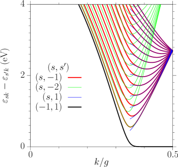
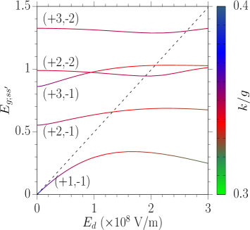
Figure 3: (a) The energy difference $\varepsilon_{sk}-\varepsilon_{s^{\prime}}$ for different $(s,s^{\prime})$ pairs at zero gate field. (b) The gate field dependence of the energy gaps $E_{g;ss^{\prime}}$ between different bands $(s,s^{\prime})$. The line color indicates the $k$ values of these gaps. The black dotted line gives the energy difference $\varepsilon_{(1)g/2}-\varepsilon_{(-1)g/2}$.

We turn to the numerical evaluation of the injection coefficients in Eq. (23) and the shift conductivity in Eq. (25). During the numerical evaluation, the Brillouin zone is divided into a $3100$ grid, the $\delta$ function is approximated by a Gaussian function

$$\delta(\hbar\omega_{s_{1}s_{2}k}-\hbar\omega)\rightarrow\frac{1}{\sqrt{\pi}\Delta}e^{-(\hbar\omega_{s_{1}s_{2}k}-\hbar\omega)^{2}/\Delta^{2}}$$ (33)

with a broadening width $\Delta=2$ meV, and the temperature is chosen at room temperature. The functions $\delta(\hbar\omega_{ss^{\prime}k}-\hbar\omega)$ are associated with the joint density of states, which gives the weight to the optical transition from the $s^{\prime}$ band to the $s$ band. It can be evaluated exactly as

$$\delta(\hbar\omega_{ss^{\prime}k}-\hbar\omega)=\sum_{j}\frac{1}{\hbar|\Delta_{ss^{\prime}k}|}\delta(k-k_{j})\,,$$ (34)

with $k_{j}$ satisfying $\omega_{ss^{\prime}k_{j}}=\omega$.

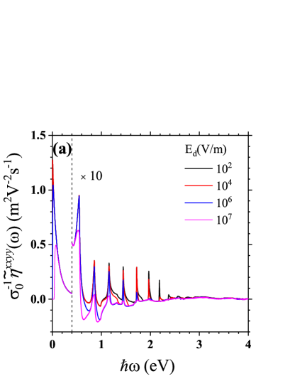
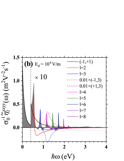
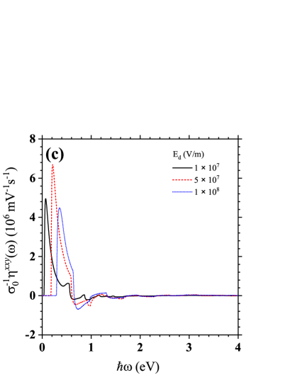
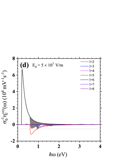
Figure 4: (a) Spectra of injection coefficient $\tilde{\eta}^{xxyy}(\omega)$ for a $24$-zGNR for gates fields $E_{d}=10^{2}$, $10^{4}$, $10^{6}$,and $10^{7}$ V/m at room temperature; the curves at the right of the vertical dashed line are scaled by 10 times. (b) The spectra of $\tilde{\eta}_{(+1)(-1)}^{xxyy}$ and $\tilde{\eta}_{l}^{xxyy}$ for $l=2,3,\cdots,8$ for $E_{d}=10^{2}$ V/m. Two specific labels mark the separated contribution of transition from band $\pm 1$ to the band l = 3. (c) The injection coefficient $\eta^{xxy}$ of zGNR under large electric field $E_{d}=10^{7}$, $5\times 10^{7}$, and $10^{8}$ V/m at room temperature. (d) The spectra of $\tilde{\eta}_{l}^{xxy}$ for $l=2,3,\cdots,8$ for $E_{d}=5\times 10^{7}$ V/m

In Fig. 3(a) the energy differences $\hbar\omega_{ss^{\prime}k}$ are plotted with respect to $k$ for different band pairs $(s,s^{\prime})$ with the condition that $|f_{sk}-f_{s^{\prime}k}|\sim 1$. The energy differences $\hbar\omega_{s(-1)k}$ and $\hbar\omega_{s(-2)k}$ show valleys around $k\sim g/3$ for all $s>1$, while $\hbar\omega_{s(+1)k}$ shows valleys only for bands with $s\geq 6$. These valleys determine the transition edge between these bands and lead to divergent joint density of states from Eq. (34). However, there is no such point for $\hbar\omega_{(+1)(-1)k}$ at zero gate field. For nonzero gate field, $\hbar\omega_{(+1)(-1)k}$ shows a valley at around similar k value $\sim g/3$, as discussed above. In Fig. 3(b), the gaps between these band pairs are plotted as functions of the gate field, and the color bar shows the $k$ values of the gap. The gate field modifies the gap between the bands $(\pm 1)$ significantly.

Figure 4 gives the spectra of injection coefficients of a $24$-zGNR at different $E_{d}$. In general, the effects of a small $E_{d}$ can be treated perturbatively and the injection coefficients can be connected with a third order sheet response coefficients as

$$\eta_{s_{1}s_{2}}^{xbc}(\omega) =\tilde{\eta}_{s_{1}s_{2}}^{xbcy}(\omega)E_{d}\,.$$ (35)

Figure 4 (a) plots the spectra of $\tilde{\eta}^{xbcy}(\omega)$ for $E_{d}=10^{2},10^{4},10^{6}$ and $10^{7}$ V/m. When the photon energy is higher than the gap, the injection occurs. As the photon energy increases, the injection coefficient increases rapidly to the first peak, and afterwards it shows more peaks and the magnitude of each peak decreases with the photon energy. The first 5 peaks are located at around $\hbar\omega\sim 0.04$, $0.53$, $0.85$, $1.16$, and $1.45$ eV; they slightly depend on the broadening parameter $\Delta$ because the Dirac function is approximated by a Gaussian function. When the photon energy is higher than $2.5$ eV, the injection coefficients are about zero. As the field $E_{d}$ increases from $10^{2}$ V/m to $10^{7}$ V/m, the value of $\tilde{\eta}^{xbxy}(\omega)$ changes little for photon energies in certain windows ($\hbar\omega\in[0.2,0.4]$ eV and a small energy range around 0.5 eV). Such energy window is enlarged to $[0.1,0.6]$ eV if the gate field $E_{d}$ is between $10^{2}$ V/m and $10^{6}$ V/m. The existence of these windows identifies the photon energies that the pertrubative treatment in Eq. (35) is appropriate. However, for photon energies $\hbar\omega>1$ eV, although the injection coefficients are small, they differ significantly even for $E_{d}=10^{2}$ V/m and $10^{4}$ V/m, indicating a non-perturbative feature of zGNR under electric fields.

The peaks are mostly induced by the optical transitions associated with the edge bands $s=\pm 1$, as shown in Fig. 4(b), where the spectra of $\tilde{\eta}^{xxyy}_{(+1)(-1)}(\omega)$ and $\tilde{\eta}_{l}=\tilde{\eta}_{l(+1)}^{xxyy}+\tilde{\eta}_{l(-1)}^{xxyy}+\tilde{\eta}_{(+1)(-l)}^{xxyy}+\tilde{\eta}_{(+1)(-l)}^{xxyy}$ are plotted for $E_{d}=10^{4}$ V/m. The electron-hole symmetry ensures $\tilde{\eta}_{s_{1}s_{2}}^{xxyy}=\tilde{\eta}_{-s_{2}-s_{1}}^{xxyy}$ for an undoped ribbon. To better understand these nonperturbative features, from Eq. (23), we write the injection coefficient as

$$\tilde{\eta}_{s_{1}s_{2}}^{xxyy}(\omega)=\frac{e^{3}}{E_{d}W\hbar^{2}}\sum_{j}\text{sgn}(\Delta^{x}_{s_{1}s_{2}k_{j}})\text{Im}[r^{y}_{s_{2}s_{1}k_{j}}r^{x}_{s_{1}s_{2}k_{j}}]f_{s_{2}s_{1}k_{j}}\,,$$ (36)

where $k_{j}$ are solutions of $\omega_{s_{1}s_{2}k_{j}}-\omega=0$ and $\text{sgn}(x)$ is a sign function. In Eq. (36) shows that the joint density of states are cancelled out with the carrier velocity. For the contribution from the transitions between the $s$th edge band and other bands $l\neq\pm 1$, the coefficients can be obtained using the results in Appendix A as

$$\tilde{\eta}_{ls}^{xxyy}(\omega) =\frac{e^{3}}{E_{d}W\hbar^{2}}\frac{s}{2}\sum_{j}\sqrt{1-N_{k_{j}}^{2}}\text{Im}[\xi_{s^{\prime}lk_{j}}^{0;x}\xi_{(-s^{\prime})lk_{j}}^{0;y}](-f_{sk_{j}})$$ (37)

As an example, the spectra of $\tilde{\eta}_{(+3)(+1)}$ and $\tilde{\eta}_{(+3)(-1)}$ are shown in Fig. 4 (b). Their values are nearly opposite thus their sum is much smaller, which indicates an interesting cancellation between the transitions. Because the nearly degenerate edge bands, the dependence on $E_{d}$ of the injection coefficients is complicated.

For higher gate fields, the band structures are dramatically changed, and the understanding of the current injection cannot be based on the quantities of ungated ribbons. The contribution from $\tilde{\eta}_{s(+1)}$ becomes negligible because there is less occupuation on the band $s=1$. Figures 4(c,d) give the spectra of $\eta^{xxy}(\omega)$ at $E_{d}=10^{7}$, $5\times 10^{7}$, and $10^{8}$ V/m. For low photon energy, the injection occurs between the bands $s=-1$ and $s=1$. As the electric field increases from $10^{7}$ to $10^{8}$ V/m, the injection coefficients keep almost unchanged, instead, the peak position changes significantly, indicating the changes of the band structure. Similar to the cases at small gate fields, the injection coefficients decrease with the photon energy quickly.

We give an estimation on how large the injection current can be at a gate field $10^{6}$ V/m. At the photon energy 0.55 eV around the second peak, our calculated current injection rate is about 0.1 m²V^-2s^-1, it corresponds to the bulk current injection rate $\sim 2\times 10^{10}$ $\mu$As^-1V^-2 considering the 0.3 nm thickness of zGNR, which is nearly 25 times larger than that in bulk GaAsPhysRevB.74.035201 . In this case, a laser pulse with intensity 0.1 GW/cm² and duration 1 ps can generate an injection current $\sim$1.1 $\mu$A.

III.3 Shift conductivity of $24$-zGNR

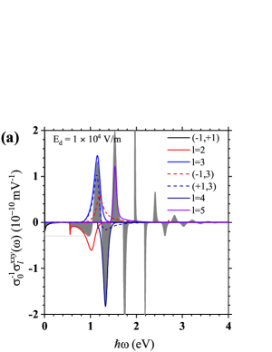
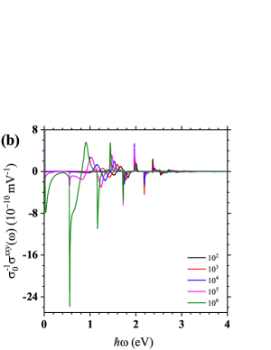
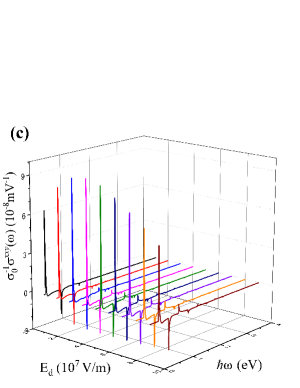
Figure 5: Spectra of shift conductivity $\sigma^{xxy}(\omega)$ for an undoped $24$-zGNR at different gate fields. (a) Transition resolved contribution of $\sigma^{xxy}(\omega)$ at $E_{d}=10^{4}$ V/m. The shadowed region gives the total conductivity. The plotted contribution from different band pairs are $\sigma^{xxy}_{(+1)(-1)}(\omega)$, $\sigma^{xxy}_{(+3)(\pm 1)}(\omega)$, as well as ${\sigma}^{xxy}_{l}(\omega)=\sum_{\pm}{\sigma}^{xxy}_{(+l)(\pm 1)}(\omega)+{\sigma}^{xxy}_{(\pm 1)(-l)}(\omega)$ for $l=2,3,4,5$. (b) Spectra of $\sigma^{xxy}(\omega)$ at $E_{d}=10^{2}$, $10^{3}$, $10^{4}$, $10^{5}$, and $10^{6}$ V/m at room temperature. (c) Spectra of $\sigma^{xxy}(\omega)$ at gate fields up to $10^{8}$ V/m.

Figure 5 (a) gives spectra of $\sigma^{xxy}(\omega)$ as well as the contributions from different optical transitions for a gate field $E_{d}=10^{4}$ V/m. The spectra show the following features: (1) The values of the shift conductivity decrease quickly with the photon energy for $\hbar\omega<0.5$ eV, and drop suddenly at $\hbar\omega\sim 0.55$ eV to a very sharp valley, which is induced by the divergent joint density of states between the bands $\pm 1$ and $\pm 2$. (2) With increasing the photon energy, the conductivity shows positive peaks and negative valleys alternatively. The first four valleys locate at $0.97$, $1.33$, $1.74$, and $2.19$ eV, and the first four peaks locate at $1.15$, $1.53$, $1.97$, and $2.41$ eV; other peaks and valleys have much smaller amplitudes. (3) The peaks and valleys have different widths, and the widths for the third peak and the fourth valley are very narrow. These peaks and valleys can be better understood from transition resolved conductivities, which are also plotted in Fig. 5 (a) for $\sigma^{xxy}_{(+1)(-1)}(\omega)$, $\sigma^{xxy}_{(+3)(\pm 1)}(\omega)$, as well as ${\sigma}^{xxy}_{l}(\omega)=\sum_{\pm}{\sigma}^{xxy}_{(+l)(\pm 1)}(\omega)+{\sigma}^{xxy}_{(\pm 1)(-l)}(\omega)$ for $l=2,3,4,5$. Similar to the injection processes, $\sigma_{(+s)(+s^{\prime})}^{xxy}(\omega)=\sigma_{(-s^{\prime})(-s)}^{xxy}(\omega)$ holds for an undoped ribbon. However, different from the injection process, the values of $\sigma_{(+s)(\pm 1)}^{xxy}$ and $\sigma_{(\pm 1)(-s)}^{xxy}$ have similar amplitudes and same signs but locate at different photon energies, and their total contribution leads to a wider peak or valley comparing those in the injection coefficients shown in Fig. 4 (b). The transition $\sigma^{xxy}_{2}$ is composed of two valleys: one is at lower photon energy, which is induced by the divergent joint density of states at 0.56 eV, and the other is at higher photon energy around 1 eV.

In Fig. 5 (b) the shift conductivities for $E_{d}=10^{2}$, $10^{3}$, $10^{5}$, and $10^{6}$ V/m are plotted for a comparison. Similar to the injection processes, the shift conductivities for photon energies lower than 0.6 eV are mostly contributed from the transition between two edge bands, and they are linearly proportional to the gate field. As the gate field $E_{d}$ increases from $10^{2}$ V/m to $10^{6}$ V/m, the location of the first valley does not change because of the negligible bandgap shift, but the peak value increases linearly from $2.5\times 10^{-12}$ m²/V² to $2.5\times 10^{-8}$ m²/V². For photon energies higher than 0.6 eV, despite of 4 orders of magnitude change for the gate field, the values for the shift conductivity are almost at the same order of magnitude; this indicates a nonperturbative dependence on the gate field, which is again induced by the near degeneracy of the edge states. Besides, the locations of peaks and valleys shift to lower photon energies as the gate field increases. Figure 5 (c) gives the spectra of the shift conductivity for gate field up to $1\times 10^{8}$ V/m. For large $E_{d}$, the values around the first two peaks are much larger; the first peak value shows a maximum around $E_{d}=4\times 10^{7}$ V/m, while the value of the second valley changes little.

As the case of injection current, we estimate the magnitude of the shift current of zGNR for a gate field $10^{6}$ V/m. At the photon energy 0.56 eV around one of the valleys, the sheet shift conductivity is $1.57\times 10^{-13}$ AmV^-2. It corresponds to the bulk photocurrent conductivity $524\ \mu$AV^-2, which is twice larger than that in 2D GeSe ($200\ \mu$AV^-2). PhysRevLett.119.067402 A laser intensity 0.1 GW/cm² can generate a shift current $\sim$0.29 $\mu$A, a few times smaller than injection currents.

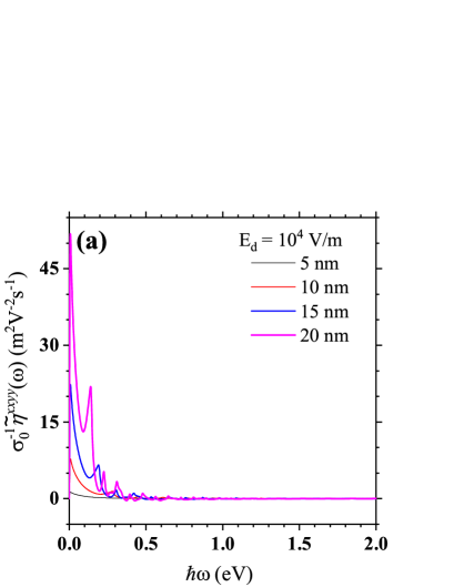
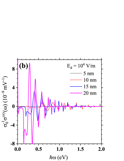
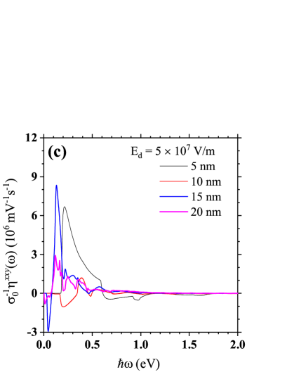
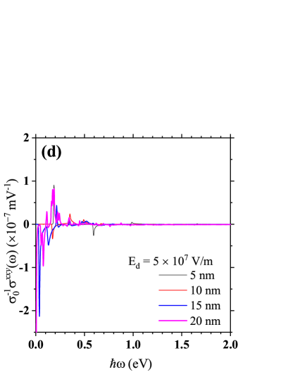
Figure 6: The spectra of injection coefficients and shift conductivities for different ribbon width $W=5$, $10$, $15$, and $20$ nm. (a) $\tilde{\eta}^{xxy}(\omega)$ at $E_{d}=10^{4}$ V/m, (b) $\sigma^{xxy}(\omega)$ at $E_{d}=10^{4}$ V/m, (c) $\tilde{\eta}^{xxy}(\omega)$ at $E_{d}=5\times 10^{7}$ V/m, (b) $\sigma^{xxy}(\omega)$ at $E_{d}=5\times 10^{7}$ V/m.

IV Width dependence

Figure 6 gives injection coefficients and shift conductivities for zGNR with different widths $W=$ 5,10,15,and 20 nm (corresponding to $N=$24,48,72 and 96) at two gate fields $E_{d}=10^{4}$ V/m and $5\times 10^{7}$ V/m. With the increase of the ribbon width, there appear more subbands, and the energy difference of neighbour bands decreases. Therefore, both for the injection coefficients and for shift conductivities, there exist more peaks or valleys in the spectra with the increase of the ribbon width, while their amplitudes change little. A wider ribbon can generate larger currents.

V Conclusion

Based on a simple tight binding model, we explored the one-color injection currents and shift currents in zigzag graphene nanoribbons, where a gate field across the ribbon is applied to break the inversion symmetry. The gate field lifts the degeneracy of the edge bands and significantly modifies their wave functions, which leads to the nonperturbative behavior with respect to even very weak gate field. The spectra of injection coefficients and shift conductivities show fruitful structures, including many peaks and valleys, with locations strongly depending on the ribbon width. These fine structures indicate the importance of the contributions from different bands. The injection coefficients are almost positive for different photon energies, while the sign of the shift conductivities is very sensitive on the photon energies. Under excitation by a pulsed laser with intensity 0.1 GW/cm², our calculation for a 5 nm wide zGNR shows that the injection current reaches $\sim$1.1 $\mu$A for a pulse with duration 1 ps, whereas the shift current is $\sim$0.29 $\mu$A. Because the injection current and the shift current can be separately excited using light with different polarization, and their magnitudes can be well tuned by the static electric field strength, these features could be experimentally observed.

Appendix A Berry connections of edge states

When there is no gate field, the wave functions can be chosen to satisfy

$$\xi_{(+1)(-1)k}^{0;x} =0\,,$$ (38)

$$\xi_{(+1)(-1)k}^{0;y} =\xi_{(-1)(+1)k}^{0;y}\text{ as real numbers}\,.$$ (39)

From Fig. 2 we have calculated the results of the left hand side of

$${\cal R}_{smk}^{0;cx}-\partial_{k}r_{smk}^{0;c}=i(\xi_{ssk}^{0;x}-\xi_{mmk}^{0;x})r_{smk}^{0;c}\,,\text{ for }m=\pm 1,\pm 2,\cdots\,.$$ (40)

and found that all of them are zero in our numerical resolution. Thus in the following we will adopt $\xi_{ssk}^{0;x}-\xi_{llk}^{0;x}=0$ without giving an exact derivation. In the new basis of $\{|sk\rangle,|lk\rangle^{0}\}$, the position matrix elements are

$$\langle sk|\tilde{\bm{r}}_{k}+i\hat{\bm{x}}\partial_{k}|lk\rangle^{0} =\frac{1}{\sqrt{2}}\left[s\sqrt{1+sN_{k}}\bm{\xi}_{(+1)lk}^{0}+\sqrt{1-sN_{k}}\bm{\xi}_{(-1)lk}^{0}\right]\,.$$ (41)

With the inclusion of the gate field, the diagonal Berry connections can be written as

$$\xi^{x}_{ssk}= \langle sk|\tilde{r}^{x}_{k}+i\partial_{k}|sk\rangle=\frac{i}{2}\left[(1+sN_{k})\xi_{(+1)(+1)k}^{0;x}+(1-sN_{k})\xi^{0;x}_{(-1)(-1)k}\right]\,,$$ (42)

then we get

$$\xi^{x}_{(+1)(+1)k}-\xi^{x}_{(-1)(-1)k} =iN_{k}\left[\xi^{0;x}_{(+1)(+1)k}-\xi^{0;x}_{(-1)(-1)k}\right]=0\,.$$ (43)

The off-diagonal Berry connections are

$$\xi^{x}_{(+1)(-1)k}= \frac{i}{2}\frac{\partial_{k}N_{k}}{\sqrt{1-N_{k}^{2}}}\,,$$ (44)

$$\xi_{(+1)(-1)k}^{y}= N_{k}\xi_{(+1)(-1)k}^{0;y}\,.$$ (45)

Further we can calculate

$${\cal R}_{(+1)(-1)k}^{cx} =\partial_{k}\xi^{c}_{(+1)(-1)k}\,,$$ (46)

$${\cal R}_{slk}^{cx} =\partial_{k}\xi^{c}_{slk}\,.$$ (47)

References

- (1) R. Alaei and M. H. Sheikhi. Optical absorption of graphene nanoribbon in transverse and modulated longitudinal electric field. Fullerenes, Nanotubes and Carbon Nanostructures, 21(3):183–197, 2013.
- (2) C. Attaccalite, E. Cannuccia, and M. Grüning. Excitonic effects in third-harmonic generation: The case of carbon nanotubes and nanoribbons. Physical Review B, 95:125403, Mar 2017.
- (3) D. Basu, M. J. Gilbert, L. F. Register, S. K. Banerjee, and A. H. MacDonald. Effect of edge roughness on electronic transport in graphene nanoribbon channel metal-oxide-semiconductor field-effect transistors. Applied Physics Letters, 92(4), 2008.
- (4) Claire Berger, Zhimin Song, Tianbo Li, Xuebin Li, Asmerom Y. Ogbazghi, Rui Feng, Zhenting Dai, Alexei N. Marchenkov, Edward H. Conrad, Phillip N. First, and Walt A. de Heer. Ultrathin epitaxial graphite: 2d electron gas properties and a route toward graphene-based nanoelectronics. The Journal of Physical Chemistry B, 108(52):19912–19916, 2004.
- (5) Akash Bhatnagar, Ayan Roy Chaudhuri, Young Heon Kim, Dietrich Hesse, and Marin Alexe. Role of domain walls in the abnormal photovoltaic effect in BiFeO3. Nature Communications, 4, NOV 2013.
- (6) Farzad Bonabi and Thomas G. Pedersen. Franz-keldysh effect and electric field-induced second harmonic generation in graphene: From one-dimensional nanoribbons to two-dimensional sheet. Physical Review B, 99:045413, Jan 2019.
- (7) L. Brey and H. A. Fertig. Electronic states of graphene nanoribbons studied with the dirac equation. Physical Review B, 73:235411, 2006.
- (8) C. P. Chang, Y. C. Huang, C. L. Lu, J. H. Ho, T. S. Li, and M. F. Lin. Electronic and optical properties of a nanographite ribbon in an electric field. Carbon, 44(3):508–515, 2006.
- (9) Ling Xiu Chen, Wang Hui Shan, Cheng Xin Jiang, Chen Chen, and Hao Min Wang. Synthesis and characterization of graphene nanoribbons on hexagonal boron nitride. Acta Physica Sinica, 68(16):168102–1, 2019.
- (10) J. D. Cox and F. Javier Garcia de Abajo. Electrically tunable nonlinear plasmonics in graphene nanoislands. Nature Communications, 5(1):5725, 2014.
- (11) Joel D. Cox and F. Javier García de Abajo. Nonlinear atom-plasmon interactions enabled by nanostructured graphene. Physical Review Letters, 121:257403, Dec 2018.
- (12) Joel D. Cox, Renwen Yu, and F. Javier García de Abajo. Analytical description of the nonlinear plasmonic response in nanographene. Physical Review B, 96:045442, Jul 2017.
- (13) Sonali Das, Deepak Pandey, Jayan Thomas, and Tania Roy. The role of graphene and other 2d materials in solar photovoltaics. Advanced Materials, 31(1):1802722, 2019.
- (14) Sandra de Vega, Joel D. Cox, Fernando Sols, and F. Javier García de Abajo. Strong-field-driven dynamics and high-harmonic generation in interacting one dimensional systems. Physical Review Research, 2:013313, Mar 2020.
- (15) Sudipta Dutta, S. Lakshmi, and Swapan K. Pati. Electron-electron interactions on the edge states of graphene: A many-body configuration interaction study. Physical Review B, 77:073412, Feb 2008.
- (16) M.M. Glazov and S.D. Ganichev. High frequency electric field induced nonlinear effects in graphene. Physics Reports, 535(3):101 – 138, 2014. High frequency electric field induced nonlinear effects in graphene.
- (17) E. Hendry, P. J. Hale, J. Moger, A. K. Savchenko, and S. A. Mikhailov. Coherent nonlinear optical response of graphene. Physical Review Letters, 105:097401, Aug 2010.
- (18) Han Hsu and L. E. Reichl. Selection rule for the optical absorption of graphene nanoribbons. Physical Review B, 76:045418, Jul 2007.
- (19) Julen Ibañez Azpiroz, Ivo Souza, and Fernando de Juan. Directional shift current in mirror-symmetric . Physical Review Research, 2:013263, Mar 2020.
- (20) J. Jiang, W. Lu, and J. Bernholc. Edge states and optical transition energies in carbon nanoribbons. Physical Review Letters, 101:246803, Dec 2008.
- (21) F. Karimi, A. H. Davoody, and I. Knezevic. Nonlinear optical response in graphene nanoribbons: The critical role of electron scattering. Physical Review B, 97:245403, Jun 2018.
- (22) Kyu Won Lee and Cheol Eui Lee. Transverse electric field-induced quantum valley hall effects in zigzag-edge graphene nanoribbons. Physics Letters A, 382(32):2137 – 2143, 2018.
- (23) M. P. López-Sancho and M. C. Muñoz. Intrinsic spin-orbit interactions in flat and curved graphene nanoribbons. Physical Review B, 83:075406, Feb 2011.
- (24) Yan Lu, Wengang Lu, Wenjie Liang, and Hong Liu. Energy splitting and optical activation of triplet excitons in zigzag-edged graphene nanoribbons. Physical Review B, 88:165425, Oct 2013.
- (25) B. S. Monozon and P. Schmelcher. Exciton absorption spectra in narrow armchair graphene nanoribbons in an electric field. Physical Review B, 99:165415, Apr 2019.
- (26) Kyoko Nakada, Mitsutaka Fujita, Gene Dresselhaus, and Mildred S. Dresselhaus. Edge state in graphene ribbons: Nanometer size effect and edge shape dependence. Physical Review B, 54:17954–17961, Dec 1996.
- (27) F. Nastos and J. E. Sipe. Optical rectification and shift currents in gaas and gap response: Below and above the band gap. Physical Review B, 74:035201, Jul 2006.
- (28) Tonatiuh Rangel, Benjamin M. Fregoso, Bernardo S. Mendoza, Takahiro Morimoto, Joel E. Moore, and Jeffrey B. Neaton. Large bulk photovoltaic effect and spontaneous polarization of single-layer monochalcogenides. Physical Review Letters, 119:067402, Aug 2017.
- (29) Hassan Raza and Edwin C. Kan. Armchair graphene nanoribbons: Electronic structure and electric-field modulation. Physical Review B, 77:245434, Jun 2008.
- (30) K. A. Ritter and J. W. Lyding. The influence of edge structure on the electronic properties of graphene quantum dots and nanoribbons. Nature Materials, 8(3):235–42, 2009.
- (31) Pascal Ruffieux, Jinming Cai, Nicholas C. Plumb, Luc Patthey, Deborah Prezzi, Andrea Ferretti, Elisa Molinari, Xinliang Feng, Klaus Müllen, Carlo A. Pignedoli, and Roman Fasel. Electronic structure of atomically precise graphene nanoribbons. ACS Nano, 6(8):6930–6935, 2012. PMID: 22853456.
- (32) C. Salazar, J. L. Cheng, and J. E. Sipe. Coherent control of current injection in zigzag graphene nanoribbons. Physical Review B, 93:075442, 2016.
- (33) V. A. Saroka, K. G. Batrakov, V. A. Demin, and L. A. Chernozatonskii. Band gaps in jagged and straight graphene nanoribbons tunable by an external electric field. Journal of Physics Condensed Matter, 27(14):145305, Apr 2015.
- (34) V. A. Saroka, M. V. Shuba, and M. E. Portnoi. Optical selection rules of zigzag graphene nanoribbons. Physical Review B, 95:155438, Apr 2017.
- (35) J. E. Sipe and A. I. Shkrebtii. Second-order optical response in semiconductors. Physical Review B, 61(8):5337–5352, 2000.
- (36) Young Woo Son, Marvin L. Cohen, and Steven G. Louie. Energy gaps in graphene nanoribbons. Physical Review Letters, 97:216803, Nov 2006.
- (37) C. G. Tao, L. Y. Jiao, O. V. Yazyev, Y. C. Chen, J. J. Feng, X. W. Zhang, R. B. Capaz, J. M. Tour, A. Zettl, S. G. Louie, H. J. Dai, and M. F. Crommie. Spatially resolving edge states of chiral graphene nanoribbons. Nature Physics, 7(8):616–620, 2011.
- (38) Katsunori Wakabayashi, Mitsutaka Fujita, Hiroshi Ajiki, and Manfred Sigrist. Electronic and magnetic properties of nanographite ribbons. Physical Review B, 59:8271–8282, Mar 1999.
- (39) Kai Wang, Rodrigo A. Muniz, J. E. Sipe, and S. T. Cundiff. Quantum interference control of photocurrents in semiconductors by nonlinear optical absorption processes. Physical Review Letters, 123:067402, Aug 2019.
- (40) Yichao Wang and David R. Andersen. First-principles study of the terahertz third-order nonlinear response of metallic armchair graphene nanoribbons. Physical Review B, 93:235430, Jun 2016.
- (41) Yichao Wang and David R Andersen. Nonlinear THz response of metallic armchair graphene nanoribbon superlattices. Journal of Physics D: Applied Physics, 49(46):46LT01, oct 2016.
- (42) Yichao Wang and David R Andersen. Third-order terahertz response of gapped, nearly-metallic armchair graphene nanoribbons. Journal of Physics: Condensed Matter, 28(47):475301, sep 2016.
- (43) Jiaqi Wu, Yinghui Zheng, Zhinan Zeng, and Ruxin Li. High-order harmonic generation from zigzag graphene nanoribbons. China Optical Letters, 18(10):103201, Oct 2020.
- (44) Shinji Yamashita. Nonlinear optics in carbon nanotube, graphene, and related 2d materials. APL Photonics, 4(3):034301, 2019.
- (45) Li Yang, Marvin L. Cohen, and Steven G. Louie. Excitonic effects in the optical spectra of graphene nanoribbons. Nano Letters, 7(10):3112–3115, 2007. PMID: 17824720.
- (46) Li Yang, Marvin L. Cohen, and Steven G. Louie. Magnetic edge-state excitons in zigzag graphene nanoribbons. Physical Review Letters, 101:186401, Oct 2008.
- (47) Sara Zamani and Rouhollah Farghadan. Graphene Nanoribbon Spin-Photodetector. PHYSICAL REVIEW APPLIED, 10(3), SEP 26 2018.
- (48) Sara Zamani and Rouhollah Farghadan. Electric field induced enhancement of photovoltaic effects in graphene nanoribbons. Physical Review B, 99:235418, Jun 2019.