Solutions of the imploding shock problem in a medium with varying density

Abstract

We consider the solutions of the Guderley problem, consisting of an imploding strong shock wave in an ideal gas with a power law initial density profile. The self-similar solutions, and specifically the similarity exponent which determines the behavior of the accelerating shock, are studied in detail, for cylindrical and spherical symmetries and for a wide range of the adiabatic index and the spatial density exponent. We then demonstrate how the analytic solutions can be reproduced in Lagrangian hydrodynamic codes, thus demonstrating their usefulness as a code validation and verification test problem.

I Introduction

The imploding shock problem, studied first by Guderly [7], involves a strong converging shock in a uniform ideal gas. It has long been considered one of the fundamental one-dimensional problems in compressible hydrodynamic flow [40, 11]. In particular, it is well known that the flow structure settles on a self-similar solution [13, 12, 20, 40, 28, 18, 25, 38, 15].

From a practical perspective, an imploding shock is a possible driving mechanism for initiating detonation in combustional material, since the shock velocity increases as it propagates inward. This possibility has several interesting prospects, such as in astrophysics [1, 2, 31] and in inertial confinement fusion [35]. In fact, as demonstrated by Kushnir et al. [10], initiation strongly depends on the ratio of shock radius to shock velocity during implosion, creating a threshold that can be assessed from the pure hydrodynamic solution.

A thorough investigation and solution of the Guderly problem was carried out by Lazarus [12, 13]. The general approach to the solution of the shock velocity, as well as the downstream density profile, is to transform the system of partial differential equations governing the motion (the Euler equations) into a system of ordinary differential equations (the self-similar equations), by introducing a self-similar variable. The similarity exponent describing the flow is then found by requiring the solution to pass through a sonic point without generating a singularity. This is an example of a "second-type" self-similar solution, which is also reflected by the fact that the exponents of the flow cannot be deduced by dimensional analysis (as opposed, for example, to the well known Sedov-Taylor explosion problem [29, 33, 4, 5, 17, 26, 9, 39, 6]).

The extensive survey [12, 13] on an imploding shock in a uniform medium examined the solutions for a wide range of values of the adiabatic index of the medium, $\gamma$, and the dimensionality (cylindrical or spherical). While other works [28, 30, 34] have considered some aspects of an imploding shock wave in a power law density profile of the form $\rho_{0}r^{\mu}$ for $\mu\geq 0$, a comprehensive survey of this generalized Guderley problem has not been carried out, and this is one of our goals here. We systematically generalize the algorithms developed by Lazarus for numerical calculations of the similarity exponent of an imploding shock in a spatial power law density profile. This algorithm is then used to conduct a semi-analytic survey of the flow for a wide range of values for $\gamma$ and for both positive and negative values of $\mu$.

A highly attractive aspect of the Guderley problem is that it offers a nontrivial test problem for hydrodynamic code verification. This was demonstrated recently in several studies [20, 23, 24, 21, 22, 19, 27, 32], for a uniform density medium. The converging nature of the flow, coupled with compression and shock discontinuity, present unique subtleties, and is therefore very useful for code validation and verification, given that the results can be compared to solutions obtained by self-similar methods. Here we expand on this point and present numerical methods and analysis of the imploding shock in a power-law density profile. In particular we present comparisons between the semi-analytic solutions and the numerical simulations for a variety of $\gamma$ and $\mu$.

We note that the full Guderley problem is actually two-fold, and also includes the reflected shock from the center. This shock can be described by a second set of self-similar solutions [12, 13], which can again be useful in code test problems [20], thus combining converging and diverging flow.

The structure of the article is as follows. In section II we review the Guderley problem, by presenting the equations, notation and conventions we use. In section III we describe the self-similar representation of the problem, derive the self-similar equations and analyze the their singular points. A robust algorithm for the calculation of the similarity exponent and the self-similar profiles for general values of $\mu$ is developed. We present the resulting similarity exponent for a wide range of values of $\gamma$ and $\mu$, and also compare the results to previously published works when such exist. Turning our focus to numerical simulation of imploding shocks, in section IV a test problem for hydrodynamic codes is developed by properly defining the initial and boundary condition of a piston with velocity given from the analytic solution [21], and examine the accessible accuracy of the solution. We conclude in section V. The main text is followed by several appendices. Details on the iterative algorithm for calculating the similarity exponent are discussed in Appendix A, which in turn depends on a critical value of the adiabatic exponents, described in Appendix B. For completeness, the calculation of approximate similarity exponents are given in Appendix C, and the numerical hydrodynamic Lagrangian scheme is laid out in Appendix D.

II The Guderley Problem

We summarize the general setting of the Guderley problem, involving a strong shock wave propagating from $r=\infty$ through an ideal gas medium, which is initially cold and at rest. The shock wave converges on an axis (in cylindrical symmetry) or a point (in spherical symmetry). The Euler equations, which govern the flow variables of the gas are:

$$\frac{\partial\rho}{\partial t}+\frac{\partial\left(\rho u\right)}{\partial r}+\left(n-1\right)\frac{\rho u}{r}=0,$$ (1)

$$\frac{\partial u}{\partial t}+u\frac{\partial u}{\partial r}+\frac{c^{2}}{\gamma\rho}\frac{\partial\rho}{\partial r}+2c\frac{\partial c}{\partial r}=0,$$ (2)

$$\frac{\partial c}{\partial t}+u\frac{\partial c}{\partial r}+\frac{\gamma-1}{2}c\left(\frac{\partial u}{\partial r}+\frac{\left(n-1\right)u}{r}\right)=0,$$ (3)

where $\rho$ denotes the fluid density, $u$ the velocity, $c$ the sound speed,and $n$ the symmetry constant ($n=2$ for cylindrical symmetry and $n=3$ for spherical symmetry). The material is assumed to be an ideal gas with an adiabatic index $\gamma$, so that the equation of state is:

$$p=\left(\gamma-1\right)\rho e,$$ (4)

relating the pressure $p$ to the specific internal energy $e$ and density $\rho$. The sound speed is then:

$$c^{2}=\frac{\gamma p}{\rho}.$$ (5)

Across the strong shock wave, the Euler equations (1)-(3) are not valid, and the strong-shock Rankine–Hugoniot relations [40] set boundary conditions for the flow variables in the shocked region:

$$\frac{\rho_{\text{shocked}}}{\rho_{0}r_{\text{shock}}^{\mu}}=\frac{\gamma+1}{\gamma-1},$$ (6)

$$u_{\text{shocked}}=\frac{2}{\gamma+1}D,$$ (7)

$$c_{\text{shocked}}=-\frac{\sqrt{2\gamma\left(\gamma-1\right)}}{\gamma+1}D,$$ (8)

where $r_{\text{shock}}$ is the shock position, and $D$ is the shock velocity.

III The Self-Similar Formulation

In deriving the self-similar solution we follow the notation and formulation set forth by Lazarus [12, 13]. The shock position is assumed to have a power law temporal dependence:

$$r_{\text{shock}}(t)=A\left(-t\right)^{\frac{1}{\lambda}},$$ (9)

where $\lambda$ is the similarity exponent. It is customary to set $A=1$, so that $r_{\text{shock}}=1$ at $t=-1$, so that convergence, $r_{\text{shock}}=0$, occurs at $t=0$. The dimensionless independent variable is set as:

$$x=\frac{t}{r^{\lambda}},$$ (10)

so that the shock position is given by $x=-1$.

In this work we study the solutions for a medium with an initial spatial power-law density profile of the form:

$$\rho(r,t=-\infty)=\rho_{0}r^{\mu}.$$

A subtlety exists for sufficiently negative values of $\mu$. We consider here the range $\mu\geq-n$, for which the mass enclosed by the shock is finite, even though the density diverges for $r\rightarrow 0$. As shown in Ref. [16], self-similar solutions do exist also for $\mu<-n$, and in fact include a transition at some $\mu_{b}<-n$ to shocks that converge at infinite times as they propagate through a steep density gradient.

The self-similar nature of the flow variables is postulated in the form:

$$u(r,t)=-\frac{r}{\lambda t}V(x),$$ (11)

$$c(r,t)=-\frac{r}{\lambda t}C(x),$$ (12)

$$\rho(r,t)=\rho_{0}r^{\mu}R(x),$$ (13)

where $V(x),C(x),R(x)$ are the similarity functions. Inserting equations (11)-(13) into the Euler equations (1)-(3) and employing the relations $\partial f/\partial r=-\lambda xr^{-1}\partial f/\partial x$, $\ \ \ \partial f/\partial t=xt^{-1}\partial f/\partial x$, results in the a system of nonlinear ordinary differential equations (ODEs) for $V(x),\ C(x)$ and $R(x)$:

$$\boldsymbol{A}\frac{d}{dx}\left[\begin{array}[]{c}R\\ V\\ C\end{array}\right]=\left[\begin{array}[]{c}V(\mu+n)\\ R\left(C^{2}(2+\mu)+\gamma V(\lambda+V)\right)\\ \frac{C\left(2\left(V+\lambda\right)+n(\gamma-1)\right)}{2\gamma(1+V)}\end{array}\right],$$ (14)

with $\boldsymbol{A}$ being the matrix:

$$\boldsymbol{A}=\lambda x\left[\begin{array}[]{ccc}\frac{1+V}{R}&1&0\\ C^{2}&\gamma R(V+1)&2RC\\ 0&\frac{C(\gamma-1)}{2\gamma(V+1)}&\frac{1}{\gamma}\end{array}\right].$$

The derivatives can be readily inverted by employing Kramers’ law. The result is commonly written as:

$$\lambda xR^{\prime}=\frac{\Delta_{1}}{\Delta},\ \ \lambda xV^{\prime}=\frac{\Delta_{2}}{\Delta},\ \ \lambda xC^{\prime}=\frac{\Delta_{3}}{\Delta},$$ (15)

with the following discriminants,

$$\Delta(V,C)=(V+1)^{2}-C^{2},$$ (16)

$$\Delta_{1}(R,V,C,\lambda,\mu) =R\Bigg{[}\frac{2(1-\lambda)+\mu(\gamma V+1)}{\gamma(V+1)}C^{2}$$

$$+V(V+\lambda)-(n+\mu)V(V+1)\Bigg{]},$$ (17)

$$\Delta_{2}(V,C,\lambda,\mu) =C^{2}\left(nV+\frac{2(\lambda-1)-\mu}{\gamma}\right)$$

$$\ \ \ \ -V(V+1)(V+\lambda),$$ (18)

$$\Delta_{3}(V,C,\lambda,\mu) =C\Bigg{[}C^{2}\left(1+\frac{2(\lambda-1)+\mu(\gamma-1)}{2\gamma(1+V)}\right)$$

$$\ \ \ \ -(V+1)^{2}-(n-1)(\gamma-1)\frac{V(1+V)}{2}$$

$$\ \ \ \ -(\lambda-1)\frac{(3-\gamma)V+2}{2}\Bigg{]}.$$ (19)

A single differential equation for $C\left(V\right)$ is then obtained from the set of equations (15):

$$\frac{dC}{dV}=\frac{\Delta_{3}(V,C,\lambda,\mu)}{\Delta_{2}(V,C,\lambda,\mu)}.$$ (20)

This equation (20) lends to integration from the known values at the shock front, for which the self-similar functions (11)-(13) are determined through the strong shock jump relations (6)-(8):

$$R_{s}\equiv R\left(-1\right)=\frac{\gamma+1}{\gamma-1},$$ (21)

$$V_{s}\equiv V\left(-1\right)=-\frac{2}{\gamma+1},$$ (22)

$$C_{s}\equiv C\left(-1\right)=\frac{\sqrt{2\gamma(\gamma-1)}}{\gamma+1}.$$ (23)

Since for $r\rightarrow\infty$ (for which $x\rightarrow 0$) the pressure and velocity are finite, it is evident from equations (11)-(12), that:

$$V_{\infty}\equiv V\left(0\right)=0,$$ (24)

$$C_{\infty}\equiv C\left(0\right)=0.$$ (25)

Hence, the two points $(V_{s},C_{s})$ and $(V_{\infty},C_{\infty})$, must be connected continuously in the $C-V$ plane by the $C\left(V\right)$ curve, with the full path obtained by integrating eq. (20). Since $\gamma>1$, the point $\left(V_{s},C_{s}\right)$ lies above the line $C=V+1$, and the solution of eq. (20) must intersect with this line as the integration advances to $\left(V_{\infty},C_{\infty}\right)$ which corresponds to the origin, as shown in Fig. 1 (and also in Figs. (2)-(3) below). Given that, at some point along the profile $C\left(V\right)$, we must have $C=V+1$, for which $\Delta=0$, and equations (15)-(20) are singular. This singularity is removable only if the intersection point satisfies $\Delta_{1}=\Delta_{2}=\Delta_{3}=0$ as well. This requirement is a constraint which enables the determination of the similarity exponent $\lambda$.

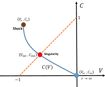
Figure 1: Illustration of the integration of eq. (20) in the $C-V$ plane. As explained in the text, the integration of the $C(V)$ curve (blue line) starts from the shock (brown point, equations (22)-(23), passes through the singular point (in red), which is the intersection point of $C(V)$ with the line $C=V+1$ (orange dotted line), and continues to the origin (blue point, equations (24)-(25)).

III.1 The Critical Points of the Similarity Equations

In order to obtain an expression for the removable singular point, which we denote by $(V_{int},C_{int})$, we set $\Delta_{2}=0$ and substitute the relation $C^{2}=(V+1)^{2}$ in eq. (18). The result is the following cubic equation for the intersection point:

$$\Bigg{[}\left(1+\frac{(\gamma-1)(1-\lambda)-\mu}{\gamma(n-1)}\right)V_{int}$$

$$\ \ +V_{int}^{2}+\frac{2(\lambda-1)-\mu}{\gamma(n-1)}\Bigg{]}\left(V_{int}+1\right)=0.$$ (26)

The root $V_{int}=-1$ is not physical since it corresponds to $C_{int}=0$, which implies zero pressure. Therefore, the two possible roots are:

$$V_{\mp}= \mp\left[\frac{1}{4}\left(\frac{\gamma-2-\frac{\mu}{\lambda-1}}{\gamma(n-1)}-1\right)^{2}-\frac{\left(2-\frac{\mu}{\lambda-1}\right)\left(\lambda-1\right)}{\gamma\left(n-1\right)}\right]^{1/2}$$

$$+\frac{\gamma-2-\frac{\mu}{\lambda-1}}{2\gamma(n-1)}-\frac{1}{2}.$$ (27)

It can be shown [13] that the correct root should be chosen according to:

$$V_{int}=\begin{cases}V_{-},&\gamma<\gamma_{crit}\\ V_{+},&\gamma\geq\gamma_{crit}\end{cases}$$ (28)

with the corresponding value of $C$ being:

$$C_{int}=V_{int}+1.$$ (29)

The critical adiabatic constant, $\gamma_{crit}=\gamma_{crit}\left(\mu,n\right)$, is defined as the value of $\gamma$ for which the discriminant of the quadratic equation (27) is zero, that is, when $V_{+}=V_{-}$. In Appendix B, we describe in detail the numerical method for calculating $\gamma_{crit}\left(\mu,n\right)$.

As shown below, assessing the $L_{int}\equiv C^{\prime}\left(V_{int}\right)$ at the singular point serves as a useful quantity for identifying the correct solution to the differential equation (20). To this end, we define $c=C-C_{int}$, $v=V-V_{int}$ and expand $\Delta_{2}$ and $\Delta_{3}$ around the singularity (where $\Delta_{2}\left(V_{int},C_{int}\right)=\Delta_{3}\left(V_{int},C_{int}\right)=0$) in eq. (20):

$$L_{int}\approx\frac{v\frac{\partial\Delta_{3}}{\partial V}+c\frac{\partial\Delta_{3}}{\partial C}}{v\frac{\partial\Delta_{2}}{\partial V}+c\frac{\partial\Delta_{2}}{\partial C}}.$$ (30)

Since $L_{int}\approx c/v$, eq. (30) reduces to a quadratic form:

$$\frac{\partial\Delta_{2}}{\partial C}L_{int}^{2}+\left(\frac{\partial\Delta_{2}}{\partial V}-\frac{\partial\Delta_{3}}{\partial C}\right)L_{int}-\frac{\partial\Delta_{3}}{\partial V}=0.$$ (31)

As shown in [13], only one of the roots of this quadratic relation corresponds to the imploding shock problem, so that the slope at the intersection point is:

$$L_{int}=\frac{\frac{\partial\Delta_{3}}{\partial C}-\frac{\partial\Delta_{2}}{\partial V}-\sqrt{\left(\frac{\partial\Delta_{3}}{\partial C}-\frac{\partial\Delta_{2}}{\partial V}\right)^{2}+4\frac{\partial\Delta_{2}}{\partial C}\frac{\partial\Delta_{3}}{\partial V}}}{2\frac{\partial\Delta_{2}}{\partial C}},$$ (32)

where the partial derivatives are evaluated at $\left(V_{int},C_{int}\right)$, and can be calculated analytically by differentiating equations (18)-(19) as follows:

$$\frac{\partial\Delta_{2}}{\partial V}=nC^{2}-V(V+1)-V(V+\lambda)-(V+1)(V+\lambda),$$ (33)

$$\frac{\partial\Delta_{2}}{\partial C}=2C\left(\frac{2(\lambda-1)-\mu}{\gamma}+nV\right),$$ (34)

$$\frac{\partial\Delta_{3}}{\partial V} =-\Bigg{[}2(1+V)+\frac{(3-\gamma)(\lambda-1)}{2}$$

$$\ \ \ \ \ \ \ +\frac{2(\lambda-1)+(\gamma-1)\mu}{2\gamma\left(V+1\right)^{2}}C^{2}$$

$$\ \ \ \ \ \ \ +(n-1)(\gamma-1)\left(V+\frac{1}{2}\right)\Bigg{]}C,$$ (35)

$$\frac{\partial\Delta_{3}}{\partial C} =3C^{2}\left(1+\frac{2(\lambda-1)+\mu(\gamma-1)}{2\gamma(1+V)}\right)$$

$$\ \ \ +(V+1)^{2}+(\lambda-1)\frac{(3-\gamma)V+2}{2}$$

$$\ \ \ -(\gamma-1)(n-1)\frac{V(V+1)}{2}.$$ (36)

III.2 Calculation of the similarity exponent

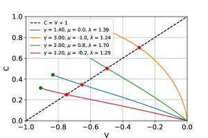
Figure 2: $C\left(V\right)$ curves obtained from integration of eq. (20) with the correct value of the similar exponent $\lambda$ for various cases with $n=3$, as detailed in the legend, where the exact value of $\lambda$ is also given. The integration starts from the shock front $\left(V_{s},C_{s}\right)$ (in green), and continues smoothly through the singularity point $\left(V_{int},C_{int}\right)$ (in red), which is the intersection with the $C=V+1$ line (dashed black line), until it reaches the origin (at $\left(V_{\infty},C_{\infty}\right)$ which corresponds to $r\rightarrow\infty$).

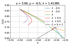
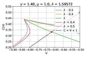
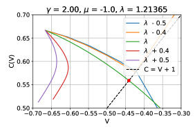
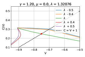
Figure 3: $C\left(V\right)$ curves for several cases (for $n=3$, and parameters which are given in the titles), each calculated with the exact similarity exponent $\lambda$ (green line), as well incorrect exponents $\lambda\pm 0.5$ (blue and purple lines) and $\lambda\pm 0.4$ (orange and red lines). It is evident that only the curve integrated with the correct value of $\lambda$, intersects the line $C=V+1$ (black dashed line) in a smooth fashion.

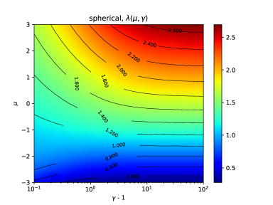
Figure 4: A color plot for the similarity exponent $\lambda$ as a function of $\gamma$ and $\mu$ for cylindrical (upper figure) and spherical (lower figure) symmetries.

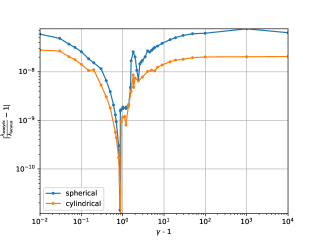
Figure 5: The relative error between the similarity exponents $\lambda$ calculated in this work and the standard results of Lazarus [13] (see tables 1-2), as a function of $\gamma$ for spherical (blue) and cylindrical (orange) symmetric flows, and $\mu=0$.

Solving the similarity exponent $\lambda$ is the main required step for calculating the similarity profiles through the ODEs in eq. (14) and the resulting flow variables via equations (11)-(13).

As discussed above, the set of equations (11)-(13) is non singular only if integration of the curve $C\left(V\right)$ (eq. (20)) intersects the line $C=V+1$ precisely at $V=V_{int}$ (eq. (28)), which will correspond to a slope $C^{\prime}\left(V_{int}\right)=L_{int}$ (eq. (32)). In Appendix A we present an iterative numerical algorithm for the calculation of $\lambda$ utilizing the fact that these conditions must be satisfied simultaneously.

Fig. 2 presents integrated $C\left(V\right)$ curves and the corresponding intersection points for various cases, calculated with the correct values of $\lambda.$ It is evident that the integration crosses the singularity in a smooth manner and reaches the origin $\left(V_{\infty},C_{\infty}\right)$ as required. In contrast, Fig. 3 compares the integration of $C\left(V\right)$ with the correct value of the similar exponent $\lambda$ to integrations with the incorrect similarity exponents $\lambda\pm 0.4$ and $\lambda\pm 0.5$. It is evident that only integrations using the correct similarity exponent pass the singular points smoothly, while integrations with incorrect similarity exponents either do not reach the $C=V+1$ line at all, or result with unphysical behaviour such as a discontinuous change of slope across the intersection.

Tables 1-2 list our results of the calculated values of $\lambda$ using the algorithm presented the special case $\mu=0$ in cylindrical and spherical symmetry, for a wide range of adiabatic exponents. The results are compared with those of published by Lazarus [13]. The relative disparity between the results is presented as a function of $\gamma$ in Fig. 5 and it is evident that an agreement to seven significant digits or better is achieved.

To the best of our knowledge, similar results were published in the past only for for some values of $\mu>0$, notably by Sharma et al. [30] and Toque [34], which we compare to our calculations in table 3. Finally, in table 4 we present numerical results of $\lambda$ for spherical and cylindrical symmetries, the typical values $\gamma=5/3,1.4$ and various different values of $\mu$, including $\mu<0$. In Fig. 4, color plots for $\lambda\left(\gamma,\mu\right)$ for a wide range of $\gamma,\mu$ are shown for spherical and cylindrical symmetries. Further support for our results was found after this work had been completed by [16].

As can be expected, $\lambda$ is a monotonically increasing function of both $\gamma$ and $\mu$. We note in passing that for $\gamma\gg 1$, the similarity exponent approaches a constant value (which depends on $\mu$), as was already noted by Lazarus [12].

$\gamma$	$\lambda_{\text{Lazarus}}$	$\lambda$
$1.01$	$1.05539838$	$1.05539835$
$1.03$	$1.08507376$	$1.08507379$
$1.05$	$1.10238925$	$1.10238927$
$1.07$	$1.11506921$	$1.11506923$
$1.1$	$1.12962686$	$1.12962688$
$1.15$	$1.14757733$	$1.14757734$
$1.2$	$1.16122032$	$1.16122033$
$1.3$	$1.18172136$	$1.18172136$
$1.4$	$1.19714143$	$1.19714143$
$1.5$	$1.20955913$	$1.20955913$
$\frac{5}{3}$	$1.22605379$	$1.22605379$

$\gamma$	$\lambda_{\text{Lazarus}}$	$\lambda$
$1.7$	$1.22889310$	$1.22889310$
$1.8$	$1.23670552$	$1.23670552$
$1.9$	$1.24362784$	$1.24362784$
$1.92$	$1.24492082$	$1.24492082$
$2$	$1.24982448$	$1.24982448$
$2.0863$	$1.25468301$	$1.25468301$
$2.0883$	$1.25479079$	$1.25479079$
$2.125$	$1.25673437$	$1.25673437$
$2.2$	$1.26049898$	$1.26049898$
$2.3676$	$1.26806432$	$1.26806432$
$2.3678$	$1.26807272$	$1.26807272$

$\gamma$	$\lambda_{\text{Lazarus}}$	$\lambda$
$2.4$	$1.26940764$	$1.26940764$
$2.6$	$1.27698161$	$1.27698162$
$2.8$	$1.28351397$	$1.28351398$
$2.8392$	$1.28469123$	$1.28469124$
$2.83929$	$1.28469390$	$1.28469391$
$3$	$1.28921366$	$1.28921367$
$3.4$	$1.29869509$	$1.29869510$
$4$	$1.30952673$	$1.30952674$
$5$	$1.32204998$	$1.32204999$
$6$	$1.33056278$	$1.33056279$
$7$	$1.33673018$	$1.33673020$

$\gamma$	$\lambda_{\text{Lazarus}}$	$\lambda$
$8$	$1.34140548$	$1.34140549$
$10$	$1.34802513$	$1.34802515$
$15$	$1.35699098$	$1.35699100$
$20$	$1.36153562$	$1.36153564$
$30$	$1.36612239$	$1.36612242$
$50$	$1.36982259$	$1.36982261$
$100$	$1.37261589$	$1.37261592$
$1000$	$1.37514328$	$1.37514331$
$9999$	$1.37539672$	$1.37539675$

Table 1: Comparison of the values of the similarity exponent $\lambda$ calculated in this work and those calculated by Lazarus [13], for different values of $\gamma$ and $\mu=0$, in cylindrical symmetry.

$\gamma$	$\lambda_{\text{Lazarus}}$	$\lambda$
$1.01$	$1.10881007$	$1.10881001$
$1.03$	$1.16716916$	$1.16716922$
$1.05$	$1.20156643$	$1.20156647$
$1.07$	$1.22695814$	$1.22695818$
$1.1$	$1.25632911$	$1.25632914$
$1.15$	$1.29284049$	$1.29284052$
$1.2$	$1.32075654$	$1.32075656$
$1.3$	$1.36281235$	$1.36281237$
$1.4$	$1.39436078$	$1.39436079$
$1.5$	$1.41959135$	$1.41959136$
$1.6$	$1.44052881$	$1.44052882$
$\frac{5}{3}$	$1.45269272$	$1.45269272$

$\gamma$	$\lambda_{\text{Lazarus}}$	$\lambda$
$1.7$	$1.45832858$	$1.45832858$
$1.8$	$1.47372274$	$1.47372274$
$1.86$	$1.48201847$	$1.48201847$
$1.88$	$1.48464620$	$1.48464620$
$1.9$	$1.48720971$	$1.48720972$
$2$	$1.49914683$	$1.49914683$
$2.01$	$1.50026616$	$1.50026616$
$2.012$	$1.50048851$	$1.50048851$
$2.2$	$1.51937505$	$1.51937505$
$2.2215$	$1.51130884$	$1.51130884$
$2.2217$	$1.52132663$	$1.52132664$
$2.4$	$1.53589867$	$1.53589867$

$\gamma$	$\lambda_{\text{Lazarus}}$	$\lambda$
$2.55194$	$1.54657142$	$1.54657143$
$2.6$	$1.54966637$	$1.54966640$
$2.8$	$1.56131989$	$1.56131993$
$3$	$1.57131262$	$1.57131266$
$3.2$	$1.57997558$	$1.57997560$
$3.4$	$1.58755678$	$1.58755679$
$3.6$	$1.59424597$	$1.59424599$
$3.8$	$1.60019098$	$1.60019100$
$4$	$1.60550871$	$1.60550874$
$4.5$	$1.61663097$	$1.61663100$
$5$	$1.62542433$	$1.62542437$
$5.5$	$1.63254761$	$1.63254766$

$\gamma$	$\lambda_{\text{Lazarus}}$	$\lambda$
$6$	$1.63843333$	$1.63843337$
$6.5$	$1.64337694$	$1.64337699$
$7$	$1.64758710$	$1.64758715$
$8$	$1.65437385$	$1.65437391$
$10$	$1.66375840$	$1.66375846$
$15$	$1.67605129$	$1.67605136$
$20$	$1.68210044$	$1.68210053$
$30$	$1.68808305$	$1.68808315$
$50$	$1.69282046$	$1.69282056$
$100$	$1.69634476$	$1.69634486$
$1000$	$1.69949536$	$1.69949549$
$9999$	$1.69980930$	$1.69980941$

Table 2: Comparison of the values of the similarity exponent $\lambda$ calculated in this work and those calculated by Lazarus [13], for different values of $\gamma$ and $\mu=0$, in spherical symmetry.

$\gamma$	$\mu$	$\lambda_{\text{Sharma}}$	$\lambda$
$1.2$	$0.5$	$1.2458754$	$1.2458735$
$\frac{5}{3}$	$0.5$	$1.3415641$	$1.3415624$
$2.0$	$0.5$	$1.3749395$	$1.3749381$
$1.2$	$1.0$	$1.3281454$	$1.3280348$
$\frac{5}{3}$	$1.0$	$1.4527030$	$1.4527000$
$2.0$	$1.0$	$1.4949825$	$1.4949798$
$1.1$	$2.0$	$1.3932402$	$1.3932370$
$1.2$	$2.0$	$1.4886240$	$1.4886198$
$1.4$	$2.0$	$1.5914957$	$1.5914907$
$\frac{5}{3}$	$2.0$	$1.6682122$	$1.6682070$
$2.0$	$2.0$	$1.7270734$	$1.7270682$
$3.0$	$2.0$	$1.8181848$	$1.8176319$
$6.0$	$2.0$	$1.9065023$	$1.9064994$

$\gamma$	$\mu$	$\lambda_{\text{Sharma}}$	$\lambda$
$1.2$	$0.5$	$1.4041700$	$1.4041673$
$\frac{5}{3}$	$0.5$	$1.4964265$	$1.4964238$
$2.0$	$0.5$	$1.5691222$	$1.5691202$
$1.2$	$1.0$	$1.4859164$	$1.4859128$
$\frac{5}{3}$	$1.0$	$1.5957192$	$1.5957154$
$2.0$	$1.0$	$1.6816074$	$1.6816040$
$1.1$	$2.0$	$1.5177710$	$1.5177653$
$1.2$	$2.0$	$1.6465296$	$1.6465223$
$1.4$	$2.0$	$1.7895314$	$1.7895229$
$\frac{5}{3}$	$2.0$	$1.8997554$	$1.8997468$
$2.0$	$2.0$	$1.9865095$	$1.9865016$
$3.0$	$2.0$	$2.1228456$	$2.1228406$
$6.0$	$2.0$	$2.2571023$	$2.2571027$

Table 3: Comparison of the of the similarity exponent $\lambda$ calculated in this work and those calculated by Sharma et al. [30], for different values $\gamma$ and $\mu>0$, in cylindrical (left table) and spherical (right table) symmetry.

$\gamma=\frac{5}{3}$
$\mu$	$\lambda_{n=2}$	$\lambda_{n=3}$
$-1$	$0.96265849$	$1.19582757$
$-0.25$	$1.16563261$	$1.39227335$
$0.5$	$1.34156241$	$1.56912017$
$1.25$	$1.50723161$	$1.73682914$
$2$	$1.66820698$	$1.89974683$

$\gamma=1.4$
$\mu$	$\lambda_{n=2}$	$\lambda_{n=3}$
$-1$	$0.96426155$	$1.17286279$
$-0.25$	$1.14366554$	$1.34177491$
$0.5$	$1.29970718$	$1.49642378$
$1.25$	$1.44745345$	$1.64464959$
$2$	$1.59149071$	$1.78952289$

Table 4: The similarity exponent for canonical values $\gamma=\frac{5}{3}$ (left table) and $\gamma=1.4$ (right table) and various values of $\mu$, in cylindrical and spherical symmetries.

III.3 Calculation of the similarity profiles

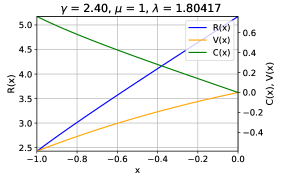
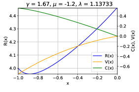
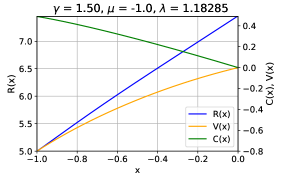
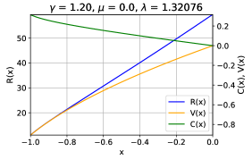
Figure 6: The similarity profiles $R\left(x\right)$ (blue line, left $y$ axis), $V\left(x\right)$ (orange line, right $y$ axis) and $C\left(x\right)$ (green line, right $y$ axis), in spherical symmetry, for different values of $\mu$ and $\gamma$, as specified in the title of each sub-figure (where the value of the similarity exponent $\lambda$ is also given).

Once the correct value of the similarity exponent is obtained, the integration of the system of differential equations (15) for the similarity profiles $R(x),V(x)$ and $C(x)$ can be performed. Integration of eq. (15) from the shock front at $x=-1$ with the initial values (see equations (21)-(23)) can, in principle be completed all the way to $x=0$ (which corresponds to $r\rightarrow\infty$). The ODE integration is performed via the LSODA integrator [8]. Numerical examples of the similarity profiles $R(x),V(x),C(x)$ for several values of $\gamma$ and $\mu$ in spherical symmetry are presented in Fig. 6.

IV Comparison to numerical simulations

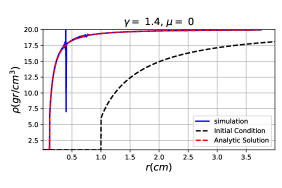
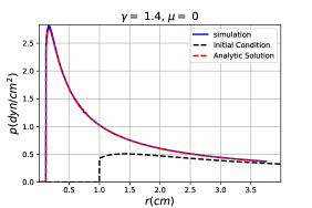
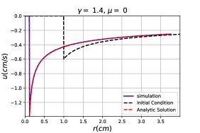
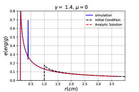
Figure 7: A comparison of hydrodynamic profiles (density, pressure, velocity and specific internal energy), resulting from numerical simulations (in blue) and the corresponding analytic solutions (in red) for $\gamma=1.4,\ \mu=0$. The simulations were performed with $N=1000$ cells. The dashed black lines describe the profiles that were used to initialize the simulations.

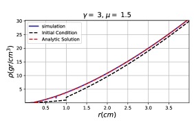
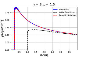
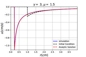
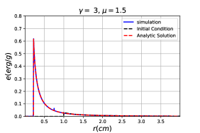
Figure 8: Same as Fig. 7, for $\gamma=3,\ \mu=1.5$.

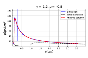
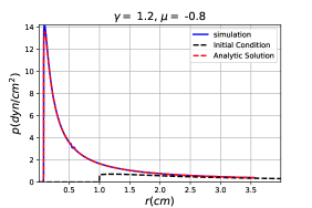
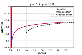
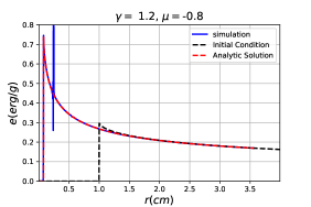
Figure 9: Same as Fig. 7, for $\gamma=1.2,\ \mu=-0.8$

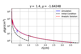
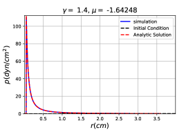
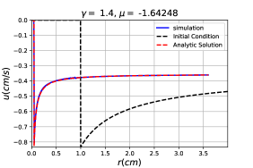
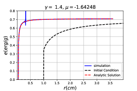
Figure 10: Same as Fig. 7, for $\gamma=1.4,\ \mu=-1.64248$

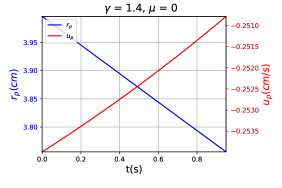
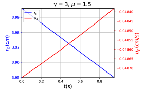
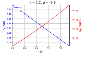
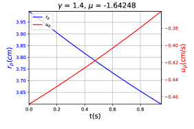
Figure 11: The piston boundary conditions as a function of time, for the four cases detailed in the text (and also in figures 7-10). The piston position is given in blue on the left y axis and the piston velocity is given in red on the right y axis.

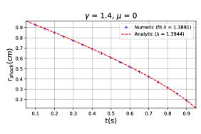
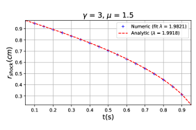
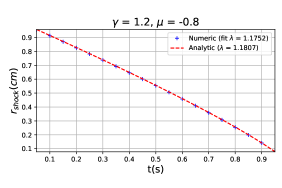
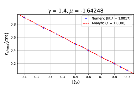
Figure 12: Comparison of the numerical (blue crosses) and analytical (red line) shock positions as a function of time, for the four cases detailed in the text (and also in figures 7-10). The numerical fitted value, and the analytic value of the similarity exponent $\lambda$, are given in the legend.

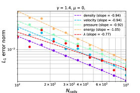
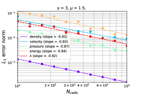
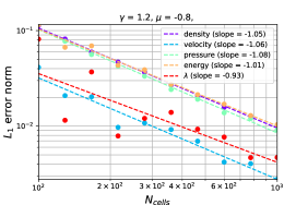
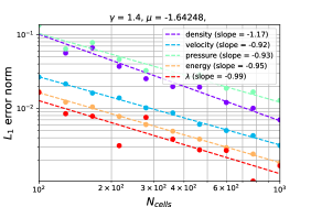
Figure 13: Convergence plots of the $L_{1}$ norm of the density (purple), velocity (blue), pressure (green) and specific internal energy (orange), and for the relative error in $\lambda$ (red), with respect to the analytical solution. The convergence rates, which are obtained from the slope of a linear fit (shown as a dashed line) on a log-log scale, are given in the legend.

We now turn to compare the semi-analytic solutions derived above with one dimensional hydrodynamic simulations. Our goal is to demonstrate that through a proper choice of initial and boundary conditions, the known solutions of the imploding shock problem can serve as a test problem for numerical codes simulating compressible flow.

IV.1 Initial and Boundary Conditions

The Guderley problem is defined as a shock converging from infinity, and application of a computational grid with a finite extent requires some adaptation. In principle, the simulation can be initialized as a Riemann problem at some large radius, with an inner region with zero pressure and velocity, and an outer region with some positive pressure. Indeed, such an initial setup will create a strong shock converging towards the origin, and the flow will asymptotically approach the analytic solution, but only up to the sonic point, where the flow is truly self-similar (independent of the details of the initial conditions).

In order to accurately describe the flow in all points in space at all times, we use a different approach to initialize the simulation. This method was described by Ramsey et al. in [20] for an Eulerian hydrodynamic calculation and later in [21] for a Lagrangian calculation. In this approach the simulation is initialized with the hydrodynamic profiles (density, velocity and pressure), given by the analytic solution for the entire spatial range at a specific time $t_{0}$. We follow the Lagrangian method, in which a moving-piston boundary condition at the outer radius is employed. The time dependent velocity of the piston, $u_{p}(t)$, is given by

$$u_{p}\left(t\right)=u_{\text{analytic}}\left(r_{p}\left(t\right),t\right),$$ (37)

where $r_{p}\left(t\right)$ is the time-dependent position of the piston, and $u_{\text{analytic}}$ is given by the analytic solution, eq. (11). Naturally, the numerical implementation is the discrete analog of eq. (37), applied at every time step to the outermost vertex on the Lagrangian grid.

IV.2 Results and Comparisons

We implemented a standard one dimensional Lagrangian hydrodynamic scheme, which is described for completeness in Appendix D. As typical examples, in the following we present comparisons between the simulations and the corresponding analytic solutions for the following cases:

• $\gamma=1.4,\ \mu=0$ - the standard Guderley problem, a converging shock with a uniform initial density profile.

• $\gamma=3,\ \mu=1.5$ - a case study for an initial density profile that goes to zero towards the center.

• $\gamma=1.2,\ \mu=-0.8$ - a case study for an initial density profile that diverges at the center.

• $\gamma=1.4,\ \mu=-1.64248$ - a particular choice for which $\lambda=1$, corresponding to a constant shock velocity.

All simulations where performed in spherical symmetry, using a spatial grid of size $N=1000$, initialized using the analytical Guderley profiles at time $t=-1$ (where the shock is at $r=1)$, and advanced until the final time $t=-0.05$. The position and velocity of the piston throughout the simulations for the four examples are also shown in figure 11.

We begin by visually comparing the numerical and analytical solutions. Comparisons of the analytical and numerical results for the flow profiles are presented for each case in figures 7-10. Shown are the hydrodynamic primitive variables: density, pressure, velocity and specific internal energy, at the final time for the numerical and analytic solutions in each of the four cases. A very good quantitative agreement is achieved in all four examples. For comparison, the figures also include the initial conditions for each of the physical quantities. Notably, a sharp discontinuity appears in the profiles in all four cases. The discontinuity exists over a single computational cell, while the overall results of the simulations do correspond with the analytic solution on either side of the discontinuity. This phenomena, which occurs also in Eulerian simulations [20], is due to the discontinuity in of the initial profiles [14], and does not affect the overall stability and accuracy of the simulations. A detailed analysis of such initialization errors is given in Ref. [20]. The shock position as a function of time in the simulations is shown along with the analytic results for the four examples, in figure 12. An excellent fit is found to exist throughout the simulations, confirming the self-similar solutions derived in this work.

Several error measures can be applied to quantitatively assess the accuracy of our derivations, as well the numerical convergence of the simulations. Here we consider the relative $L_{1}$ error measure for the profiles at the end of the simulations, defined by

$$L_{1}=\frac{\sum_{k}\left|y_{k}-y_{k}^{\text{analytic}}\right|}{\frac{1}{2}\left(\sum_{k}\left|y_{k}\right|+\sum_{k}\left|y_{k}^{\text{analytic}}\right|\right)}$$ (38)

where $y$ and $y^{\text{analytic}}$ denote the numerical and analytical values, respectively, of the physical quantities. The index $k$ denotes the cell or vertex in the simulation, for which the analytic solution is derived through the physical location of the $k$-th cell/vertex. The quality of numerical convergence in this measure for the four simulations are shown in Fig. 13, plotted as a function of the number of numerical cells, ranging from $100$ to $1000$. While there exists some diversity in the accuracy of the simulations regarding the different physical quantities, we observe that a grid of 1000 cells will generally suffice to ensure an accuracy of a few percent or even less than one percent in all physical quantities at the end of the simulation. Accuracy is eroded, of course, for smaller grids, increasing the error to the order of ten percent in the least accurate quantities (usually the internal energy or the pressure). Notably, the convergence rates (reduction of error as a function of increase in grid size) is similar for all physical quantities in all simulations. These rates are all of order unity (see explicitly in the figures), as is to be expected for an artificial viscosity numerical scheme, which is first order accurate in the presence of shocks.

Another integral measure of relative error is the difference between the analytical value of similarity exponent and it numerical counterpart, derived by fitting the numerical shock position as a function of time to a power law of the form of eq. (9). This error measure, $\left|\lambda_{\text{numerical}}/\lambda_{\text{analytic}}-1\right|$, is also depicted in Fig. 13, and we find that it is generally as indicative of numerical convergence as the $L_{1}$ measure for the physical quantities.

V Summary

In this work we studied the Guderley problem of a strong shock imploding in an ideal gas medium with an initial power-law density profile, $\rho(r)\sim r^{\mu}$. We developed and reviewed the theoretical framework required to construct self-similar solutions for the flow. These solutions were systematically compared to numerical simulations employing a one dimensional Lagrangian hydrodynamic code, and using appropriate initial and boundary conditions.

From the physics stand point, we presented a first survey of the imploding shock problem for a wide range of parameters, notably the adiabatic constant $\gamma$ and the power of the initial density profile, $\mu$, including $\mu<0$. Our results are in excellent agreement with previous works with $\mu=0$, and with the few published cases which considered $\mu>0$ only.

We demonstrated how the semi-analytic solution can be used to initialize a nontrivial compressible flow problem which can serve for code verification. In particular, we find that the numerical solution provides near-linear convergence in terms of the $L_{1}$-norm, which bodes well for physical problems where high-accuracy is required to asses the outcome, such as double detonations in white dwarfs, sonoluminiscene and inertial confinement fusion.

By expanding the Guderley problem to non-uniform density profiles, we found a wide variability of the flow properties. This feature poses the imploding shock problem as an attractive test for hydrodynamic codes aimed at simulating compressible flow. Correspondingly, the imploding strong shock offers a verification analysis for one-dimensional compressible codes, as well as a starting point for two- and three-dimensional codes.

Finally, we call attention to the complete Guderley problem covering both the converging shock and the reflected shock which follows convergence (for times $t>0$). The reflected shock and the entire flow profile can also be solved semi-analytically in self-similar fashion. This is well known to be the case for a uniform medium, and is also applicable for non-zero values of $\mu$ covering both negative and positive values. As discussed in detail by [16], a reflected shock actually exists only for a finite range $\mu_{-}<\mu<\mu_{+}$. For $\mu<\mu_{-}$ the flow behind the converging shock stagnates as the shock advances through the steep gradient towards the origin, while for $\mu>\mu_{+}$ the diminishing density at the center causes the pressure at the origin to vanish at convergence rather than to become infinite (both $\mu_{-}$ and $\mu_{+}$, which are negative and positive, respectively, depend on $\gamma$ and the geometry of the flow). In cases where it does exist, the reflected shock marks another advantage of the Guderley problem as a test case for hydrodynamic codes, since it involves both converging and diverging flow [20]. In a follow-up work we will extend the physical and numerical analysis of the reflected shock to relevant non-zero values of $\mu$, both negative and positive, demonstrating the quality of the Guderley problem as comprehensive test of hydrodynamic codes for compressible flow through a non-uniform medium.

Availability of data

The data that support the findings of this study are available from the corresponding author upon request.

Appendix A Iterative algorithm for the calculation of the Similarity Exponent

In order to calculate the similarity exponent, $\lambda$, we construct a scalar function, $f\left(\lambda\right)$, for which the correct value of $\lambda$ is a root. As explained above in section III.1, only for the correct value of $\lambda$ does a numerical integration of the ODE (20) intersects with the line $C=V+1$ at the point $\left(V_{int},C_{int}\right)$ (as given by equations (28),(29)) and with with a slope $L_{int}$ (as given by eq. (32)). The function $f\left(\lambda\right)$ is defined below and solved by iterations as follows:

1. For a given guess for $\lambda$, calculate the values of the desired intersection point $\left(V_{int},C_{int}\right)$ using equations (28)-(29) and the slope of the $C(V)$ curve at this point, using equations (32)-(36).

2. Calculate the $C\left(V\right)$ curve, by numerically integrating eq. (20) from the shock $\left(V_{s},C_{s}\right)$ (see equations (22)-(23)) to the singular point $V=V_{int}$. The resulting value of $C$ at that point is $C\left(V_{int}\right)\equiv C_{*}$. In addition, the integration is explicitly evaluated at a point $V_{int}-\varepsilon$ close to the singular point, where $\varepsilon=\left|\frac{V_{s}-V_{int}}{V_{scale}}\right|$, and the value of $C$ is denoted by $C\left(V_{int}-\epsilon\right)\equiv C_{*}^{-}$. This gives the numerical value for the intersection point $\left(V_{int},C^{*}\right)$, and for a point close to the intersection point, $\left(V_{int}-\varepsilon,C_{*}^{-}\right)$. The ODE integration is performed via the LSODA integrator [8].

3. The numerical value for the slope near the intersection point, is evaluated as:

   $$L_{*}=\frac{dC}{dV}\left(V_{int}-\varepsilon,C_{*}^{-}\right),$$ (39)

   where $dC/dV$ is calculated using eq. (20).

4. The value returned is given by:

   $$f\left(\lambda\right)=\begin{cases}\left(C_{int}-C_{*}\right)\cdot 10^{k+\alpha}&\gamma<\gamma_{crit}\\ \left(L_{int}-L_{*}\right)\cdot 10^{k+\beta}&\gamma\geq\gamma_{crit}\end{cases}$$ (40)

   where the calculation of $\gamma_{crit}$ is explained separately below in Appendix B, and:

   $$\alpha=\log\left|L_{*}-L_{int}\right|,$$ (41)

   $$\beta=\log\left|C_{*}-C_{int}\right|.$$ (42)

The quantities $V_{scale}$ and $10^{k}$ control the quality of convergence and obviously must be chosen to be large. We find that $V_{scale}=5\cdot 10^{4}$ and $k=5$ suffice to achieve accurate and fast convergence. The root of $f\left(\lambda\right)$ is found using the bisection method, on a range $\left[\lambda_{\text{min}},\lambda_{\text{max}}\right]$ such that $f\left(\lambda_{\text{min}}\right)\cdot f\left(\lambda_{\text{max}}\right)<0.$ In order to find such a range, we use a well known approximation for the similarity exponent, denoted by $\lambda_{\text{approx}}$ (as explained in Appendix C). If $f\left(\lambda_{\text{approx}}\right)>0$, we fix $\lambda_{\text{min}}=\lambda_{\text{approx}}$, otherwise we take $\lambda_{\text{max}}=\lambda_{\text{approx}}$.

Appendix B Numerical Calculation of $\gamma_{crit}$

In this Appendix we describe the algorithm calculating $\gamma_{crit}$, used in the calculation of the similarity exponent $\lambda$. For a given $\gamma$, we integrate the ODE (20) from the shock point $\left(V_{s},C_{s}\right)$ until it intersects with the line $C=V+1$. In this integration, an approximated similarity exponent $\lambda_{approx}$ is used, as detailed in Appendix C. Once the intersection is found, the distances in the $C-V$ plane between the intersection point and the possible roots $\left(V_{\mp},C_{\mp}\right)$ are calculated. If the intersection point is closer to $\left(V_{-},C_{-}\right)$ we know that $\gamma<\gamma_{crit}$, otherwise $\gamma\geq\gamma_{crit}$. This process results in a step function of $\gamma$ centered around $\gamma_{crit}$, readily solvable via the bisection method.

Numerical results of $\gamma_{crit}$ for various values of $\mu$ are given for reference in table 5. Specifically, we note that our results for $\mu=0$, $\gamma_{cirt}=1.9092$ and $\gamma_{crit}=1.8698$ for cylindrical and spherical symmetry (respectively) are in excellent agreement with those found by Lazarus [12, 13].

$n$	$\mu$	$\gamma_{crit}$
$2$	$-1$	$1$
$2$	$-0.66$	$1.08725$
$2$	$-0.33$	$1.39453$
$2$	$0.0$	$1.90920$
$2$	$0.33$	$2.66220$
$2$	$0.66$	$3.79614$
$2$	$1.0$	$5.74731$

$n$	$\mu$	$\gamma_{crit}$
$2$	$1.33$	$9.52816$
$2$	$1.66$	$20.6303$
$3$	$-2$	$1.00004$
$3$	$-1.5$	$1.04219$
$3$	$-1$	$1.19790$
$3$	$-0.5$	$1.47479$
$3$	$0.0$	$1.86976$

$n$	$\mu$	$\gamma_{crit}$
$3$	$0.5$	$2.40285$
$3$	$1.0$	$3.12706$
$3$	$1.5$	$4.14803$
$3$	$2.0$	$5.68258$
$3$	$2.5$	$8.24007$
$3$	$3.0$	$13.3511$
$3$	$3.5$	$28.6723$

Table 5: The values of $\gamma_{crit}$ for various value of $n$ and $\mu$

Appendix C Calculation of an approximated similarity exponent $\lambda$

For completeness, we review here the simple approximation for the similarity exponent $\lambda$, developed by Chisnell for $\mu=0$ [3], and extended by Vishwakarama for $\mu\neq 0$ [36].

The variables $\alpha=\frac{1}{\lambda}$ and $V_{0}$ are coupled through a pair of equations:

$$\left(\frac{\alpha}{V_{0}}-1\right)^{2}=\frac{\gamma\left(\gamma-1\right)}{2}\left(\frac{\gamma-1}{\left(\gamma+1\right)\left(1-\frac{V_{0}}{\alpha}\right)}\right)^{\eta}\left(\frac{V_{0}+q}{\frac{2\alpha}{\gamma+1}+q}\right)^{B}$$ (43)

$$\left(n-1+\frac{\mu\alpha}{\gamma V_{0}}\right)\frac{\alpha}{1-\alpha}=\frac{1}{1-\frac{V_{0}}{\alpha}}+\frac{2\alpha}{\gamma V_{0}},$$ (44)

where:

$$\eta=\frac{2\left(1-\alpha\right)+\left(\gamma-1\right)\mu\alpha}{\alpha(n\gamma+\mu)-2\left(1-\alpha\right)},$$ (45)

$$B=\eta+\left(n-1\right)\frac{2\left(\frac{\alpha}{V_{0}}-1\right)^{2}+\gamma-1}{1-n\left(\frac{\alpha}{V_{0}}-1\right)^{2}},$$ (46)

$$q=-\frac{\alpha}{V_{0}\left(1-n\left(\frac{\alpha}{V_{0}}-1\right)^{2}\right)},$$ (47)

The equations can be simplified by defining an auxiliary variable:

$$\xi=\frac{\alpha}{V_{0}}.$$ (48)

Substituting $\xi$ and solving for $\alpha$ in eq. (44), we find:

$$\alpha\left(\xi\right)=\frac{\frac{\xi}{\xi-1}+\frac{2}{\gamma}\xi}{n-1+\frac{\mu}{\gamma}\xi+\frac{\xi}{\xi-1}+\frac{2}{\gamma}\xi},$$ (49)

Inserting this result for $\alpha\left(\xi\right)$ into eq. (43), is equivalent to finding the root of the function:

$$f\left(\xi\right) =\frac{\gamma\left(\gamma-1\right)}{2}\left(\frac{\gamma-1}{\left(\gamma+1\right)\left(1-\frac{1}{\xi}\right)}\right)^{\eta(\xi)}\left(\frac{\frac{\alpha\left(\xi\right)}{\xi}+q\left(\xi\right)}{\frac{2\alpha\left(\xi\right)}{\gamma+1}+q\left(\xi\right)}\right)^{B(\xi)}$$

$$\ \ \ \ -\left(\xi-1\right)^{2},$$ (50)

where:

$$q\left(\xi\right)=-\frac{\xi}{1-n\left(\xi-1\right)^{2}},$$ (51)

$$\eta\left(\xi\right)=\frac{2\left(1-\alpha\left(\xi\right)\right)+\left(\gamma-1\right)\mu\alpha\left(\xi\right)}{\alpha\left(\xi\right)\left(n\gamma+\mu\right)-2\left(1-\alpha\left(\xi\right)\right)},$$ (52)

$$B\left(\xi\right)=\eta\left(\xi\right)+\left(n-1\right)^{2}\frac{2\left(\xi-1\right)^{2}+\gamma-1}{1-n\left(\xi-1\right)^{2}}.$$ (53)

The root of eq. (50) is found numerically via the Newton-Raphson method with the following initial value (see in [3, 36]):

$$\xi_{0}=\sqrt{\frac{\gamma\left(\gamma-1\right)}{2}}+1.$$ (54)

Typically the root of eq. (50) is found after three or four Newton-Raphson iterations. After finding the root $\xi_{*}$ we substitute this root into eq. (49), and obtain the approximate value of the similarity exponent $\lambda_{approx}=\alpha^{-1}\left(\xi_{*}\right)$.

Appendix D The Hydrodynamic Scheme

We used a standard one dimensional staggered grid Lagrangian hydrodynamic scheme. The computational grid is divided into cells indexed $1...N$ and vertices indexed $\frac{1}{2},...N+\frac{1}{2}$. Thermodynamic variables, $\rho_{i},p_{i},e_{i},c_{i}$, are defined on cells, while kinematic variables $r_{i\pm\frac{1}{2}},u_{i\pm\frac{1}{2}},a_{i\pm\frac{1}{2}}$ (position, velocity and acceleration) are defined on vertices. The mass of each cell, $m_{i}$, is time independent, given by the initial combination of volumes, $V_{i}^{0}$, and densities $\rho_{i}^{0}$.

Denoting the number of the time step by an upper index $k$, the integration timestep, $\Delta t^{k}=t^{k+1}-t^{k}$, is chosen according to the CFL stability condition [14]:

$$\Delta t^{k}=0.16\min_{i}\left(\frac{r_{i+\frac{1}{2}}^{k}-r_{i-\frac{1}{2}}^{k}}{c_{s,i}^{k}}\right),$$ (55)

where the cell-related speed of sound is given by the ideal gas relation:

$$c_{s,i}^{k}=\left(\frac{\gamma p_{i}^{k}}{\rho_{i}^{k}}\right)^{1/2}.$$

We used a standard leap-frog temporal integration scheme, where the next values of velocity, position, volume and density of each vertex and cell are found through:

$$u_{i+\frac{1}{2}}^{k+\frac{1}{2}}=u_{i+\frac{1}{2}}^{k}+\frac{\Delta t^{k}}{2}a_{i+\frac{1}{2}}^{k},$$ (56)

$$r_{i+\frac{1}{2}}^{k+1}=r_{i+\frac{1}{2}}^{k}+\Delta t^{k}u_{i+\frac{1}{2}}^{k+\frac{1}{2}},$$ (57)

$$V_{i}^{k+1}=A\left(\left(r_{i+\frac{1}{2}}^{k+1}\right)^{n}-\left(r_{i-\frac{1}{2}}^{k+1}\right)^{n}\right),$$ (58)

$$\rho_{i}^{k+1}=\frac{m_{i}}{V_{i}^{k+1}}.$$ (59)

The geometry of the flow enters through the volume coefficient $A=1,\pi,\frac{4}{3}\pi$ and the dimensionality $n=1,2,3$ for planar, cylindrical and spherical symmetries, respectively.

Numerical stability at the shock is achieved with the commonly used Von-Neumann-Richtmyer [37] artificial viscosity:

$$q_{i}^{k+1}=\begin{cases}0&V_{i}^{k+1}\geq V_{i}^{k}\\ \sigma\rho_{i}^{k+1}\left(u_{i+\frac{1}{2}}^{k+\frac{1}{2}}-u_{i-\frac{1}{2}}^{k+\frac{1}{2}}\right)^{2},&\text{else}\end{cases}$$ (60)

taking $\sigma=3$. Finally, the specific internal energy, pressure and acceleration are solved according to:

$$e_{i}^{k+1}=\frac{e_{i}^{k}-\frac{1}{2}\left(p_{i}^{k}+q_{i}^{k+1}+q_{i}^{k}\right)\frac{V_{i}^{k+1}-V_{i}^{k}}{m_{i}}}{1+\frac{1}{2}\left(\gamma-1\right)\frac{V_{i}^{k+1}-V_{i}^{k}}{m_{i}}},$$ (61)

$$p_{i}^{k+1}=\left(\gamma-1\right)e_{i}^{k+1}\rho_{i}^{k+1},$$ (62)

$$a_{i+\frac{1}{2}}^{k+1}=-B\left(r_{i+\frac{1}{2}}^{k+1}\right)^{n-1}\frac{p_{i+1}^{k+1}+q_{i+1}^{k+1}-p_{i}^{k+1}-q_{i}^{k+1}}{\frac{1}{2}\left(m_{i+1}+m_{i}\right)},$$ (63)

where the areal coefficient is $B=1,2\pi,4\pi$ for planar, cylindrical, and spherical symmetries, respectively.

References

- [1] David Arnett and Eli Livne. The delayed-detonation model of a type ia supernovae. 1: The deflagration phase. The Astrophysical Journal, 427:315–329, 1994.
- [2] David Arnett and Eli Livne. The delayed-detonation model of type ia supernovae. 2: The detonation phase. The Astrophysical Journal, 427:330–341, 1994.
- [3] RF Chisnell. An analytic description of converging shock waves. Journal of Fluid Mechanics, 354:357–375, 1998.
- [4] Stephen V Coggeshall and Roy A Axford. Lie group invariance properties of radiation hydrodynamics equations and their associated similarity solutions. The Physics of fluids, 29(8):2398–2420, 1986.
- [5] SV Coggeshall. Analytic solutions of hydrodynamics equations. Physics of Fluids A: Fluid Dynamics, 3(5):757–769, 1991.
- [6] Tamar Faran and Re’em Sari. The non-relativistic interiors of ultra-relativistic explosions: Extension to the blandford–mckee solutions. Physics of Fluids, 33(2):026105, 2021.
- [7] KG Guderley. Starke kugelige und zylindrische verdichtungsstosse in der nahe des kugelmitterpunktes bnw. der zylinderachse. Luftfahrtforschung, 19:302, 1942.
- [8] Alan C Hindmarsh. Odepack, a systematized collection of ode solvers. Scientific computing, pages 55–64, 1983.
- [9] Menahem Krief. Analytic solutions of the nonlinear radiation diffusion equation with an instantaneous point source in non-homogeneous media. Physics of Fluids, 33(5):057105, 2021.
- [10] Doron Kushnir, Eli Livne, and Eli Waxman. Imploding ignition waves. i. one-dimensional analysis. The Astrophysical Journal, 752(2):89, 2012.
- [11] L. D. Landau and E. M. Lifshitz. Fluid Mechanics, Second Edition: Volume 6 (Course of Theoretical Physics). Course of theoretical physics / by L. D. Landau and E. M. Lifshitz, Vol. 6. Butterworth-Heinemann, 2 edition, 1987.
- [12] RB Lazarus and RD Richtmyer. Similarity solutions for converging shocks. Technical report, COLORADO UNIV AT BOULDER DEPT OF MATHEMATICS, 1977.
- [13] Roger B Lazarus. Self-similar solutions for converging shocks and collapsing cavities. SIAM Journal on Numerical Analysis, 18(2):316–371, 1981.
- [14] Randall J LeVeque et al. Finite volume methods for hyperbolic problems, volume 31. Cambridge university press, 2002.
- [15] Jürgen Meyer-ter Vehn and Christian Schalk. Selfsimilar spherical compression waves in gas dynamics. Zeitschrift für Naturforschung A, 37(8):954–970, 1982.
- [16] Elisha Modelevsky and Re’em Sari. Revisiting the strong shock problem: Converging and diverging shocks in different geometries. Physics of Fluids, 33(5):056105, 2021.
- [17] R Pakula and R Sigel. Self-similar expansion of dense matter due to heat transfer by nonlinear conduction. The Physics of fluids, 28(1):232–244, 1985.
- [18] NF Ponchaut, HG Hornung, DI Pullin, and CA Mouton. On imploding cylindrical and spherical shock waves in a perfect gas. Journal of Fluid Mechanics, 560:103, 2006.
- [19] Scott D Ramsey and Roy S Baty. Piston driven converging shock waves in a stiffened gas. Physics of Fluids, 31(8):086106, 2019.
- [20] Scott D Ramsey, James R Kamm, and John H Bolstad. The guderley problem revisited. International Journal of Computational Fluid Dynamics, 26(2):79–99, 2012.
- [21] Scott D Ramsey and Jennifer F Lilieholm. Verification assessment of piston boundary conditions for lagrangian simulation of the guderley problem. Journal of Verification, Validation and Uncertainty Quantification, 2(3), 2017.
- [22] Scott D Ramsey, Emma M Schmidt, Zachary M Boyd, Jennifer F Lilieholm, and Roy S Baty. Converging shock flows for a mie-grüneisen equation of state. Physics of Fluids, 30(4):046101, 2018.
- [23] Scott D Ramsey and Mikhail J Shashkov. Simulation and analysis of converging shock wave test problems. Technical report, Los Alamos National Lab.(LANL), Los Alamos, NM (United States), 2012.
- [24] Scott D Ramsey and Mikhail J Shashkov. Surrogate guderley test problem definition. Technical report, Los Alamos National Lab.(LANL), Los Alamos, NM (United States), 2012.
- [25] A Ramu and MP Ranga Rao. Converging spherical and cylindrical shock waves. Journal of engineering mathematics, 27(4):411–417, 1993.
- [26] P Reinicke and J Meyer-ter Vehn. The point explosion with heat conduction. Physics of Fluids A: Fluid Dynamics, 3(7):1807–1818, 1991.
- [27] JJ Ruby, JR Rygg, JA Gaffney, B Bachmann, and GW Collins. A boundary condition for guderley’s converging shock problem. Physics of Fluids, 31(12):126104, 2019.
- [28] Akira Sakurai. On the problem of a shock wave arriving at the edge of a gas. Communs. Pure and Appl. Math., 13, 1960.
- [29] L. I. Sedov. Propagation of strong blast waves. Prikl. Mat. Mekh., 10:241, 1946.
- [30] VD Sharma and Ch Radha. Similarity solutions for converging shocks in a relaxing gas. International journal of engineering science, 33(4):535–553, 1995.
- [31] Ken J. Shen and Lars Bildsten. The ignition of carbon detonations via converging shocks in white dwarfs. The Astrophysical Journal, 785(2):61, 2014.
- [32] Mayank Singh, Astha Chauhan, Kajal Sharma, and Rajan Arora. Kinematics of one-dimensional spherical shock waves in interstellar van der waals gas clouds. Physics of Fluids, 32(10):107109, 2020.
- [33] G. I. Taylor. Propagation of strong blast waves. Proc. R. Soc. London, 201:159, 1950.
- [34] Nathalie Toqué. Self-similar implosion of a continuous stratified medium. Shock Waves, 11(3):157–165, 2001.
- [35] RibeyreKen X. Vallet, A. and V. Tikhonchuk. Finite mach number spherical shock wave, application to shock ignition. Physics of Plasmas, 20(2):082702, 2013.
- [36] JP Vishwakarma and Subhash Vishwakarma. An analytic description of converging shock waves in a gas with variable density. Physica Scripta, 72(2-3):218, 2005.
- [37] John VonNeumann and Robert D Richtmyer. A method for the numerical calculation of hydrodynamic shocks. Journal of applied physics, 21(3):232–237, 1950.
- [38] Robert L Welsh. Imploding shocks and detonations. Journal of Fluid Mechanics, 29(1):61–79, 1967.
- [39] Almog Yalinewich and Re’em Sari. Analytic asymptotic solution to spherical relativistic shock breakout. Physics of Fluids, 29(1):016103, 2017.
- [40] Ya B Zel’Dovich and Yu P Raizer. Physics of shock waves and high-temperature hydrodynamic phenomena. Courier Corporation, 2002.