Psycholinguistic Tripartite Graph Network for Personality Detection

Abstract

Most of the recent work on personality detection from online posts adopts multifarious deep neural networks to represent the posts and builds predictive models in a data-driven manner, without the exploitation of psycholinguistic knowledge that may unveil the connections between one’s language usage and his psychological traits. In this paper, we propose a psycholinguistic knowledge-based tripartite graph network, TrigNet, which consists of a tripartite graph network and a BERT-based graph initializer. The graph network injects structural psycholinguistic knowledge from LIWC, a computerized instrument for psycholinguistic analysis, by constructing a heterogeneous tripartite graph. The graph initializer is employed to provide initial embeddings for the graph nodes. To reduce the computational cost in graph learning, we further propose a novel flow graph attention network (GAT) that only transmits messages between neighboring parties in the tripartite graph. Benefiting from the tripartite graph, TrigNet can aggregate post information from a psychological perspective, which is a novel way of exploiting domain knowledge. Extensive experiments on two datasets show that TrigNet outperforms the existing state-of-art model by 3.47 and 2.10 points in average F1. Moreover, the flow GAT reduces the FLOPS and Memory measures by 38% and 32%, respectively, in comparison to the original GAT in our setting.

1 Introduction

Personality detection from online posts aims to identify one’s personality traits from the online texts he creates. This emerging task has attracted great interest from researchers in computational psycholinguistics and natural language processing due to the extensive application scenarios such as personalized recommendation systems Yang and Huang (2019); Jeong et al. (2020), job screening Hiemstra et al. (2019) and psychological studies Goreis and Voracek (2019).

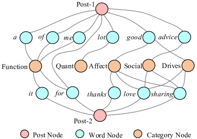
Figure 1: An example of our tripartite graph. The content of Post-1 and Post-2 are “A lot of good advise for me.” and “Love it! Thanks for sharing!”, respectively.

Psychological research shows that the words people use in daily life reflect their cognition, emotion, and personality Gottschalk (1997); Golbeck (2016). As a major psycholinguistic instrument, Linguistic Inquiry and Word Count (LIWC) Tausczik and Pennebaker (2010) divides words into psychologically relevant categories (e.g., Function, Affect, and Social as shown in Figure 1) and is commonly used to extract psycholinguistic features in conventional methods Golbeck et al. (2011); Sumner et al. (2012). Nevertheless, most recent works Hernandez and Knight (2017); Jiang et al. (2020); Keh et al. (2019); Lynn et al. (2020); Gjurković et al. (2020) tend to adopt deep neural networks (DNNs) to represent the posts and build predictive models in a data-driven manner. They first encode each post separately and then aggregate the post representations into a user representation. Although numerous improvements have been made over the traditional methods, they are likely to suffer from limitations as follows. First, the input of this task is usually a set of topic-agnostic posts, some of which may contain few personality cues. Hence, directly aggregating these posts based on their contextual representations may inevitably introduce noise. Second, personality detection is a typical data-hungry task since it is non-trivial to obtain personality tags, while DNNs implicitly extract personality cues from the texts and call for tremendous training data. Naturally, it is desirable to explicitly introduce psycholinguistic knowledge into the models to capture critical personality cues.

Motivated by the above discussions, we propose a psycholinguistic knowledge-based tripartite graph network, namely TrigNet, which consists of a tripartite graph network to model the psycholinguistic knowledge and a graph initializer using a pre-trained language model such as BERT Devlin et al. (2019) to generate the initial representations for all the nodes. As illustrated in Figure 1, a specific tripartite graph is constructed for each user, where three heterogeneous types of nodes, namely post, word, and category, are used to represent the posts of a user, the words contained both in his posts and the LIWC dictionary, and the psychologically relevant categories of the words, respectively. The edges are determined by the subordination between word and post nodes as well as between word and category nodes. Besides, considering that there are no direct edges between homogeneous nodes (e.g., between post nodes) in the tripartite graph, a novel flow GAT is proposed to only transmit messages between neighboring parties to reduce the computational cost and to allow for more effective interaction between nodes. Finally, we regard the averaged post node representation as the final user representation for personality classification. Benefiting from the tripartite graph structure, the interaction between posts is based on psychologically relevant words and categories rather than topic-agnostic context.

We conduct extensive experiments on the Kaggle and Pandora datasets to evaluate our TrigNet model. Experimental results show that it achieves consistent improvements over several strong baselines. Comparing to the state-of-the-art model, SN+Att Lynn et al. (2020), TrigNet brings a remarkable boost of 3.47 in averaged Macro-F1 (%) on Kaggle and a boost of 2.10 on Pandora. Besides, thorough ablation studies and analyses are conducted and demonstrate that the tripartite graph and the flow GAT play an irreplaceable role in the boosts of performance and decreases of computational cost.

Our contributions are summarized as follows:

• This is the first effort to use a tripartite graph to explicitly introduce psycholinguistic knowledge for personality detection, providing a new perspective of using domain knowledge.

• We propose a novel tripartite graph network, TrigNet, with a flow GAT to reduce the computational cost in graph learning.

• We demonstrate the outperformance of our TrigNet over baselines as well as the effectiveness of the tripartite graph and the flow GAT by extensive studies and analyses.

2 Related Work

2.1 Personality Detection

As an emerging research problem, text-based personality detection has attracted the attention of both NLP and psychological researchers Cui and Qi (2017); Xue et al. (2018); Keh et al. (2019); Jiang et al. (2020); Tadesse et al. (2018); Lynn et al. (2020).

Traditional studies on this problem generally resort to feature-engineering methods, which first extracts various psychological categories via LIWC Tausczik and Pennebaker (2010) or statistical features by the bag-of-words model Zhang et al. (2010). These features are then fed into a classifier such as SVM Cui and Qi (2017) and XGBoost Tadesse et al. (2018) to predict the personality traits. Despite interpretable features that can be expected, feature engineering has such limitations as it relies heavily on manually designed features.

With the advances of deep neural networks (DNNs), great success has been achieved in personality detection. Tandera et al. (2017) apply LSTM Hochreiter and Schmidhuber (1997) on each post to predict the personality traits. Xue et al. (2018) develop a hierarchical DNN, which depends on an AttRCNN and a variant of Inception Szegedy et al. (2017) to learn deep semantic features from the posts. Lynn et al. (2020) first encode each post by a GRU Cho et al. (2014) with attention and then pass the post representations to another GRU to produce the whole contextual representations. Recently, pre-trained language models have been applied to this task. Jiang et al. (2020) simply concatenate all the utterances from a single user into a document and encode it with BERT Devlin et al. (2019) and RoBERTa Liu et al. (2019). Gjurković et al. (2020) first encode each post by BERT and then use CNN LeCun et al. (1998) to aggregate the post representations. Most of them focus on how to obtain more effective contextual representations, with only several exceptions that try to introduce psycholinguistic features into DNNs, such as Majumder et al. (2017) and Xue et al. (2018). However, these approaches simply concatenate psycholinguistic features with contextual representations, ignoring the gap between the two spaces.

2.2 Graph Neural Networks

Graph neural networks (GNNs) can effectively deal with tasks with rich relational structures and learn a feature representation for each node in the graph according to the structural information. Recently, GNNs have attracted wide attention in NLP Cao et al. (2019); Yao et al. (2019); Wang et al. (2020b, a). Among these research, graph construction lies at the heart as it directly impacts the final performance. Cao et al. (2019) build a graph for question answering, where the nodes are entities, and the edges are determined by whether two nodes are in the same document. Yao et al. (2019) construct a heterogeneous graph for text classification, where the nodes are documents and words, and the edges depend on word co-occurrences and document-word relations. Wang et al. (2020b) define a dependency-based graph by utilizing dependency parsing, in which the nodes are words, and the edges rely on the relations in the dependency parsing tree. Wang et al. (2020a) present a heterogeneous graph for extractive document summarization, where the nodes are words and sentences, and the edges depend on sentence-word relations. Inspired by the above successes, we construct a tripartite graph, which exploits psycholinguistic knowledge instead of simple document-word or sentence-word relations and is expected to contribute towards psychologically relevant node representations.

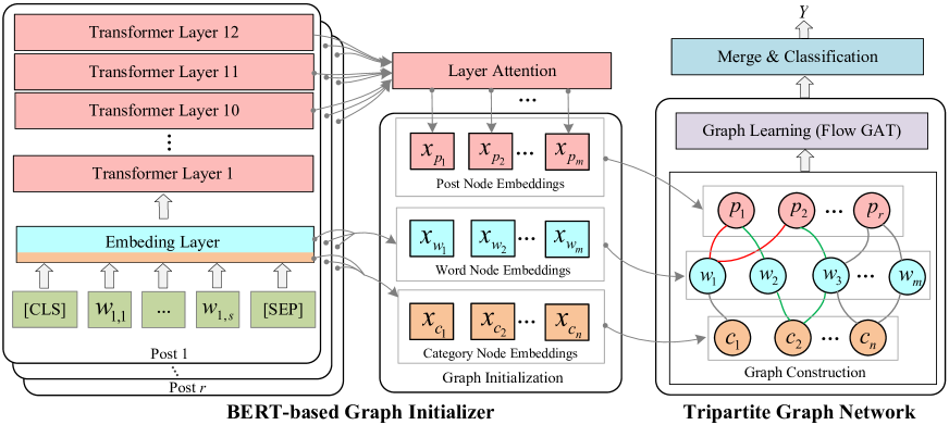
Figure 2: Overall architecture of our TrigNet, which consists of two modules: (1) a tripartite graph network (right) to inject psycholinguistic knowledge and (2) a BERT-based graph initializer (left) to initialize node embeddings.

3 Our Approach

Personality detection can be formulated as a multi-document multi-label classification task Lynn et al. (2020); Gjurković et al. (2020). Formally, each user has a set $P{\rm{=}}\left\{{{p_{1}},{p_{2}},\ldots,{p_{r}}}\right\}$ of posts. Let ${p_{i}}{\rm{=}}\left[{{w_{i,1}},{w_{i,2}},\ldots,{w_{i,s}}}\right]$ be the $i$-th post with $s$ words, where $p_{i}$ can be viewed as a document. The goal of this task is to predict $T$ personality traits $Y{\rm{=}}\left\{{{y^{t}}}\right\}_{t=1}^{T}$ for this user based on $P$, where $y^{t}\in\left\{{0,1}\right\}$ is a binary variable.

Figure 2 presents the overall architecture of the proposed TrigNet, which consists of a tripartite graph network and a BERT-based graph initializer. The former module aims to explicitly infuse psycholinguistic knowledge to uncover personality cues contained in the posts and the latter to encode each post and provide initial embeddings for the tripartite graph nodes. In the following subsections, we detail how the two modules work in four steps: graph construction, graph initialization, graph learning, and merge & classification.

3.1 Graph Construction

As a major psycholinguistic analysis instrument, LIWC Tausczik and Pennebaker (2010) divides words into psychologically relevant categories and is adopted in this paper to construct a heterogeneous tripartite graph for each user.

As shown in the right part of Figure 2, the constructed tripartite graph $\mathcal{G}{\rm{=}}\left({\mathcal{V},\mathcal{E}}\right)$ contains three heterogeneous types of nodes, namely post, word, and category, where $\mathcal{V}$ denotes the set of nodes and $\mathcal{E}$ represents the edges between nodes. Specifically, we define $\mathcal{V}{\rm{=}}{\mathcal{V}_{p}}\cup{\mathcal{V}_{w}}\cup{\mathcal{V}_{c}}$, where ${\mathcal{V}_{p}}{\rm{=}}P{\rm{=}}\left\{{{p_{1}},{p_{2}},\cdots,{p_{r}}}\right\}$ denotes $r$ posts, ${\mathcal{V}_{w}}{\rm{=}}\left\{{{w_{1}},{w_{2}},\cdots,{w_{m}}}\right\}$ denotes $m$ unique psycholinguistic words that appear both in the posts $P$ and the LIWC dictionary, and ${\mathcal{V}_{c}}{\rm{=}}\left\{{{c_{1}},{c_{2}},\cdots,{c_{n}}}\right\}$ represents $n$ psychologically relevant categories selected from LIWC. The undirected edge $e_{ij}$ between nodes $i$ and $j$ indicates word $i$ either belongs to a post $j$ or a category $j$.

The interaction between posts in the tripartite graph is implemented by two flows: (1) “$p{\rm{\leftrightarrow}}w{\rm{\leftrightarrow}}p$”, which means posts interact via their shared psycholinguistic words (e.g., “$p_{1}{\rm{\leftrightarrow}}w_{1}{\rm{\leftrightarrow}}p_{2}$” as shown by the red lines in Figure 2); (2) “$p{\rm{\leftrightarrow}}w{\rm{\leftrightarrow}}c{\rm{\leftrightarrow}}w{\rm{\leftrightarrow}}p$”, which suggests that posts interact by words that share the same category (e.g., “$p_{1}{\rm{\leftrightarrow}}w_{2}{\rm{\leftrightarrow}}c_{2}{\rm{\leftrightarrow}}w_{3}{\rm{\leftrightarrow}}p_{2}$” as shown by the green lines in Figure 2). Hence, the interaction between posts is based on psychologically relevant words or categories rather than topic-agnostic context.

3.2 Graph Initialization

As shown in the left part of Figure 2, we employ BERT Devlin et al. (2019) to obtain the initial embeddings of all the nodes. BERT is built upon the multi-layer Transformer encoder Vaswani et al. (2017), which consists of a word embedding layer and 12 Transformer layers.

Post Node Embedding   The representations at the 12-th layer of BERT are usually used to represent an input sequence. This may not be appropriate for our task as personality is only weakly related to the higher order semantic features of posts, making it risky to rely solely on the final layer representations. In our experiments (Section 5.4), we find that the representations at the 11-th and 10-th layers are also useful for this task. Therefore, we utilize the representations at the last three layers to initialize the post node embeddings. Formally, the representations ${x_{p_{i}}^{j}}$ of the $i$-th post at the $j$-th layer can be obtained by:

$${x_{p_{i}}^{j}}{\rm{=}}{{\rm{BERT}}^{j}}\left({\left[{{\rm{CLS}},{w_{i,1}},\cdots,{w_{i,m}},{\rm{SEP}}}\right]}\right)$$ (1)

where “CLS” and “SEP” are special tokens to denote the start and end of an input sentence, respectively, and ${\mathop{\rm BERT}^{j}\nolimits}\left(\cdot\right)$ denotes the representation of the special token “CLS” at the $j$-th layer. In this way, we obtain the representations ${\left[{x_{{p_{i}}}^{10},x_{{p_{i}}}^{11},x_{{p_{i}}}^{12}}\right]^{\rm{T}}}\in{\mathbb{R}^{3\times d}}$ of the last three layers, where $d$ is the dimension of each representation. We then apply layer attention Peters et al. (2018) to collapse the three representations into a single vector $x_{{p_{i}}}$:

$${x_{{p_{i}}}}=\sum\limits_{j=10}^{12}{{\alpha_{j}}x_{{p_{i}}}^{j}}$$ (2)

where $\alpha_{j}$ are softmax-normalized layer-specific weights to be learned. Consequently, we can obtain a set of post representations for the given $r$ posts of a user ${\bf X_{p}}={\left[{{x_{p_{1}}},{x_{p_{2}}},\cdots,{x_{p_{r}}}}\right]^{\rm{T}}}\in{\mathbb{R}^{r\times d}}$

Word Node Embedding  BERT applies WordPiece Wu et al. (2016) to split words, which also cuts out-of-vocabulary words into small pieces. Thus, we obtain the initial node embedding of each word in $\mathcal{V}_{w}$ by considering two cases: (1) If the word is not out of vocabulary, we directly look up the BERT embedding layer to obtain its embedding; (2) If the word is out of vocabulary, we use the averaged embedding of its pieces as its initial node embedding. The initial word node embeddings are represented as ${\bf X_{w}}{\rm{=}}{\left[{{x_{w_{1}}},{x_{w_{2}}},\cdots,{x_{w_{m}}}}\right]^{\rm{T}}}\in{\mathbb{R}^{m\times d}}$.

Category Node Embedding   The LIWC dictionary divides words into 9 main categories and 64 subcategories. Empirically, subcategories such as Pronouns, Articles, and Prepositions are not task-related. Besides, our initial experiments show that excessive introduction of subcategories in the tripartite graph makes the graph sparse and makes the learning difficult, resulting in performance deterioration. For these reasons, we select all 9 main categories and the 6 personal-concern subcategories for our study. Particularly, the 9 main categories Function, Affect, Social, Cognitive Processes, Perceptual Processes, Biological Processes, Drives, Relativity, and Informal Language, and 6 personal-concern subcategories Work, Leisure, Home, Money, Religion, and Death are used as our category nodes. Then, we replace the “UNUSED” tokens in BERT’s vocabulary by the 15 category names and look up the BERT embedding layer to generate their embeddings ${\bf X_{c}}{\rm{=}}{\left[{{x_{c_{1}}},{x_{c_{2}}},\cdots,{x_{c_{n}}}}\right]^{\rm{T}}}\in{\mathbb{R}^{n\times d}}$.

3.3 Graph Learning

Graph attention network (GAT) Veličković et al. (2018) can be applied over a graph to calculate the attention weight of each edge and update the node representations. However, unlike the traditional graph in which any two nodes may have edges, the connections in our tripartite graph only occur between neighboring parties (i.e., ${\mathcal{V}_{w}}\leftrightarrow{\mathcal{V}_{p}}$ and ${\mathcal{V}_{w}}\leftrightarrow{\mathcal{V}_{c}}$), as shown in Figure 3. Therefore, applying the original GAT over our tripartite graph will lead to unnecessary computational costs. Inspired by Wang et al. (2020a), we propose a flow GAT for the tripartite graph. Particularly, considering that the interaction between posts in our tripartite graph can be accounted for by two flows “$p{\rm{\leftrightarrow}}w{\rm{\leftrightarrow}}p$” and “$p{\rm{\leftrightarrow}}w{\rm{\leftrightarrow}}c{\rm{\leftrightarrow}}w{\rm{\leftrightarrow}}p$”, we design a message passing mechanism that only transmits message by the two flows in the tripartite graph.

Formally, given a constructed tripartite graph $\mathcal{G}=\left({\mathcal{V},\mathcal{E}}\right)$, where $\mathcal{V}={\mathcal{V}_{p}}\cup{\mathcal{V}_{w}}\cup{\mathcal{V}_{c}}$, and the initial node embeddings ${\bf X}{\rm{=}}{\bf X_{p}}{\rm{\cup}}{{\bf X_{w}}}{\rm{\cup}}{{\bf X_{c}}}$, we compute ${\bf{H}}_{\bf{p}}^{{}^{\left(l+1\right)}}$, ${\bf{H}}_{\bf{w}}^{{}^{\left(l+1\right)}}$, and ${\bf{H}}_{\bf{c}}^{{}^{\left(l+1\right)}}$ as the hidden states of $\mathcal{V}_{p}$, $\mathcal{V}_{w}$ and $\mathcal{V}_{c}$ at the $(l+1)$-th layer. The flow GAT layer is defined as follows:

$${\bf{H}}_{\bf{p}}^{{}^{\left({l+1}\right)}}{\rm{,}}{\bf{H}}_{\bf{w}}^{{}^{\left({l+1}\right)}}{\rm{,}}{\bf{H}}_{\bf{c}}^{{}^{\left({l+1}\right)}}{\rm{=FGAT}}\left({{\bf{H}}_{\bf{p}}^{{}^{\left(l\right)}}{\rm{,}}{\bf{H}}_{\bf{w}}^{{}^{\left(l\right)}}{\rm{,}}{\bf{H}}_{\bf{c}}^{{}^{\left(l\right)}}}\right)$$ (3)

where ${\bf{H}}_{\bf{p}}^{{}^{\left(1\right)}}={{\bf{X}}_{\bf{p}}}$, ${\bf{H}}_{\bf{w}}^{{}^{\left(1\right)}}={{\bf{X}}_{\bf{w}}}$, and ${\bf{H}}_{\bf{c}}^{{}^{\left(1\right)}}={{\bf{X}}_{\bf{c}}}$. The function ${\rm{FGAT}}\left(\cdot\right)$ is implemented by the two flows:

$$\begin{array}[]{l}{\bf{\hat{H}}}_{{\bf{w}}\leftarrow{\bf{p}}}^{{}^{\left(l\right)}}{\rm{=}}{\mathop{\rm MP}\nolimits}\left({{\bf{H}}_{\bf{w}}^{{}^{\left(l\right)}},{\bf{H}}_{\bf{p}}^{{}^{\left(l\right)}}}\right)\\ {\bf{H}}_{{\bf{p}}\leftarrow{\bf{w,p}}}^{{}^{\left(l\right)}}={\mathop{\rm MP}\nolimits}\left({{\bf{H}}_{\bf{p}}^{{}^{\left(l\right)}},{\bf{\hat{H}}}_{{\bf{w}}\leftarrow{\bf{p}}}^{{}^{\left(l\right)}}}\right)\end{array}$$ (4)

$$\begin{array}[]{l}{\bf{H}}_{{\bf{c}}\leftarrow{\bf{w,p}}}^{{}^{\left(l\right)}}={\mathop{\rm MP}\nolimits}\left({{\bf{H}}_{\bf{c}}^{{}^{\left(l\right)}},{\bf{\hat{H}}}_{{\bf{w}}\leftarrow{\bf{p}}}^{{}^{\left(l\right)}}}\right)\\ {\bf{H}}_{{\bf{w}}\leftarrow{\bf{c,w,p}}}^{{}^{\left(l\right)}}={\mathop{\rm MP}\nolimits}\left({{\bf{\hat{H}}}_{{\bf{w}}\leftarrow{\bf{p}}}^{{}^{\left(l\right)}},{\bf{H}}_{{\bf{c}}\leftarrow{\bf{w,p}}}^{{}^{\left(l\right)}}}\right)\\ {\bf{H}}_{{\bf{p}}\leftarrow{\bf{w,c,w,p}}}^{{}^{\left(l\right)}}={\mathop{\rm MP}\nolimits}\left({{\bf{H}}_{\bf{p}}^{{}^{\left(l\right)}},{\bf{H}}_{{\bf{w}}\leftarrow{\bf{c,w,p}}}^{{}^{\left(l\right)}}}\right)\end{array}$$ (5)

$$\begin{array}[]{l}{\bf{H}}_{\bf{p}}^{{}^{\left({l+1}\right)}}={\mathop{\rm mean}\nolimits}\left({{\bf{H}}_{{\bf{p}}\leftarrow{\bf{w,p}}}^{{}^{\left(l\right)}},{\bf{H}}_{{\bf{p}}\leftarrow{\bf{w,c,w,p}}}^{{}^{\left(l\right)}}}\right)\\ {\bf{H}}_{\bf{w}}^{{}^{\left({l+1}\right)}}={\mathop{\rm mean}\nolimits}\left({{\bf{\hat{H}}}_{{\bf{w}}\leftarrow{\bf{p}}}^{{}^{\left(l\right)}},{\bf{H}}_{{\bf{w}}\leftarrow{\bf{c,w,p}}}^{{}^{\left(l\right)}}}\right)\\ {\bf{H}}_{\bf{c}}^{{}^{\left({l+1}\right)}}={\bf{H}}_{{\bf{c}}\leftarrow{\bf{w,p}}}^{{}^{\left(l\right)}}\end{array}$$ (6)

where ${\rm{\leftarrow}}$ means the message is transmitted from the right nodes to the left nodes, ${\mathop{\rm mean}\nolimits}\left(\cdot\right)$ is the mean pooling function, and ${\mathop{\rm MP}\nolimits}\left(\cdot\right)$ represents the message passing function. Eq. (4) and Eq. (5) illustrate that message is transmitted by the flows “$p{\rm{\leftrightarrow}}w{\rm{\leftrightarrow}}p$” and $p{\rm{\leftrightarrow}}w{\rm{\leftrightarrow}}c{\rm{\leftrightarrow}}w{\rm{\leftrightarrow}}p$, respectively.

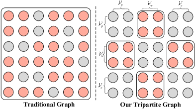
Figure 3: Comparison of adjacent matrices between the traditional graph (left) and our tripartite graph (right). Edges in the traditional graph may occur in any two nodes, while it only occurs between neighboring parties in our tripartite graph.

We take ${\mathop{\rm MP}\nolimits}\left({{\bf{H}}_{\bf{w}}^{{}^{\left(l\right)}},{\bf{H}}_{\bf{p}}^{{}^{\left(l\right)}}}\right)$ in Eq. (4) as an example to introduce the massage passing function, where ${\bf{H}}_{\bf{w}}^{{}^{\left(l\right)}}=\left[{h_{{w_{1}}}^{\left(l\right)},h_{{w_{2}}}^{\left(l\right)},\cdots,h_{{w_{m}}}^{\left(l\right)}}\right]$ are used as the attention query and ${\bf{H}}_{\bf{p}}^{{}^{\left(l\right)}}{\rm{=}}\left[{h_{{p_{1}}}^{\left(l\right)},h_{{p_{2}}}^{\left(l\right)},\cdots,h_{{p_{r}}}^{\left(l\right)}}\right]$ as the key and value. ${\mathop{\rm MP}\nolimits}\left({{\bf{H}}_{\bf{w}}^{{}^{\left(l\right)}},{\bf{H}}_{\bf{p}}^{{}^{\left(l\right)}}}\right)$ can be decomposed into three steps. First, it calculates the attention weight $\beta^{k}_{ij}$ between node $i$ in $\mathcal{V}_{w}$ and its neighbor node $j$ in $\mathcal{V}_{p}$ at the $k$-th head:

$${z^{k}_{ij}}=\sigma\left({{{\bf{W}}^{k}_{\bf{z}}}\left[{{{\bf{W}}^{k}_{\bf{w}}}h_{{w_{i}}}^{\left(l\right)}||{{\bf{W}}^{k}_{\bf{p}}}h_{{p_{j}}}^{\left(l\right)}}\right]}\right)$$ (7)

$${\beta^{k}_{ij}}=\frac{{\exp\left({{z^{k}_{ij}}}\right)}}{{\sum\nolimits_{q\in{{\cal N}_{i}}}{\exp\left({{z^{k}_{iq}}}\right)}}}$$ (8)

where $\sigma$ is the LeakyReLU activation function, ${{\bf{W}}^{k}_{\bf{z}}}$, ${{\bf{W}}^{k}_{\bf{w}}}$ and ${{\bf{W}}^{k}_{\bf{p}}}$ are learnable weights, ${\mathcal{N}}_{i}$ means that the neighbor nodes of node $i$ in $\mathcal{V}_{p}$, and $||$ is the concatenation operation. Second, the updated hidden state $\tilde{h}_{{w_{i}}}^{\left(l\right)}$ is obtained by a weighted combination of its neighbor nodes in $\mathcal{V}_{p}$:

$$\tilde{h}_{{w_{i}}}^{\left({l}\right)}=\mathop{||}\limits_{k=1}^{K}\tanh\left({\sum\limits_{j\in{\mathcal{N}_{i}}}{\beta_{ij}^{k}{\bf{W}}_{\bf{v}}^{k}h_{{p_{j}}}^{\left(l\right)}}}\right)$$ (9)

where $K$ is the number of heads and ${{\bf{W}}^{k}_{\bf{v}}}$ is a learnable weight matrix. Third, noting that the above steps do not take the information of node $i$ itself into account and to avoid gradient vanishing, we introduce a residual connection to produce the final updated node representation:

$$\hat{h}_{{w_{i}}}^{\left({l}\right)}=h_{{w_{i}}}^{\left(l\right)}+\tilde{h}_{{w_{i}}}^{\left({l}\right)}$$ (10)

3.4 Merge & Classification

After $L$ layers of iteration, we obtain the final node representations ${{{\bf{H}}^{\left(L\right)}}}{\rm{=}}{{\bf{H}}_{\bf{p}}^{{}^{\left(L\right)}}}{\rm{\cup}}{{{\bf{H}}_{\bf{w}}^{{}^{\left(L\right)}}}}{\rm{\cup}}{{{\bf{H}}_{\bf{c}}^{{}^{\left(L\right)}}}}$. Then, we merge all post node representations ${{\bf{H}}_{\bf{p}}^{{}^{\left(L\right)}}}$ via mean pooling to produce the user representation:

$$u={\rm{mean}}\left({\left[{h_{{p_{1}}}^{\left(L\right)},h_{{p_{2}}}^{\left(L\right)},\cdots,h_{{p_{r}}}^{\left(L\right)}}\right]}\right)$$ (11)

Finally, we employ $T$ softmax-normalized linear transformations to predict $T$ personality traits. For the $t$-th personality trait, we compute:

$${p\left({y^{t}}\right)}={\rm{softmax}}\left({u{\bf{W}}_{\bf{u}}^{t}+{\bf{b}}_{\bf{u}}^{t}}\right)$$ (12)

where ${{\bf{W}}_{\bf{u}}^{t}}$ is a trainable weight matrix and ${\bf{b}}_{\bf{u}}^{t}$ is a bias term. The objective function of our TrigNet model is defined as:

$$J\left(\theta\right)=\frac{1}{V}\sum\limits_{v=1}^{V}{\sum\limits_{t=1}^{T}{\left[{-y_{v}^{t}\log p\left({y_{v}^{t}|\theta}\right)}\right]}}$$ (13)

where $V$ is the number of training samples, $T$ is the number of personality traits, $y_{v}^{t}$ is the true label for the $t$-th trait, and $p({y_{v}^{t}|\theta})$ is the predicted probability for this trait under parameters $\theta$.

4 Experiments

In this section, we introduce the datasets, baselines, and settings of our experiments.

4.1 Datasets

We choose two public MBTI datasets for evaluations, which have been widely used in recent studies Tadesse et al. (2018); Hernandez and Knight (2017); Majumder et al. (2017); Jiang et al. (2020); Gjurković et al. (2020). The Kaggle dataset is collected from PersonalityCafe, where people share their personality types and discussions about health, behavior, care, etc. There are a total of 8675 users in this dataset and each user has 45-50 posts. Pandora is another dataset collected from Reddit, where personality labels are extracted from short descriptions of users with MBTI results to introduce themselves. There are dozens to hundreds of posts for each of the 9067 users in this dataset.

The traits of MBTI include Introversion vs. Extroversion (I/E), Sensing vs. iNtuition (S/N), Think vs. Feeling (T/F), and Perception vs. Judging (P/J). Following previous works Majumder et al. (2017); Jiang et al. (2020), we delete words that match any personality label to avoid information leaks. The Macro-F1 metric is adopted to evaluate the performance in each personality trait since both datasets are highly imbalanced, and average Macro-F1 is used to measure the overall performance. We shuffle the datasets and split them in a 60-20-20 proportion for training, validation, and testing, respectively. According to our statistics, there are respectively 20.45 and 28.01 LIWC words on average in each post in the two datasets, and very few posts (0.021/0.002 posts per user) are presented as disconnected nodes in the graph. We show the statistics of the two datasets in Table 1.

Dataset	Traits	Train (60%)	Valid (20%)	Test (20%)
Kaggle	I/E	4011 / 1194	1326 / 409	1339 / 396
	S/N	610 / 4478	222 / 1513	248 / 1487
	T/F	2410 / 2795	791 / 944	780 / 955
	P/J	3096 / 2109	1063 / 672	1082 / 653
Pandora	I/E	4278 / 1162	1427 / 386	1437 / 377
	S/N	727 / 4830	208 / 1605	210 / 1604
	T/F	3549 / 1891	1120 / 693	1182 / 632
	P/J	3211 / 2229	1043 / 770	1056 / 758

Table 1: Statistics of the Kaggle and Pandora datasets.

Methods	Kaggle					Pandora
	I/E	S/N	T/F	P/J	Average	I/E	S/N	T/F	P/J	Average
SVM Cui and Qi (2017)	53.34	47.75	76.72	63.03	60.21	44.74	46.92	64.62	56.32	53.15
XGBoost Tadesse et al. (2018)	56.67	52.85	75.42	65.94	62.72	45.99	48.93	63.51	55.55	53.50
BiLSTM Tandera et al. (2017)	57.82	57.87	69.97	57.01	60.67	48.01	52.01	63.48	56.21	54.93
BERT Keh et al. (2019)	64.65	57.12	77.95	65.25	66.24	56.60	48.71	64.70	56.07	56.52
AttRCNN Xue et al. (2018)	59.74	64.08	78.77	66.44	67.25	48.55	56.19	64.39	57.26	56.60
SN+Attn Lynn et al. (2020)	65.43	62.15	78.05	63.92	67.39	56.98	54.78	60.95	54.81	56.88
TrigNet(our)	69.54	67.17	79.06	67.69	70.86	56.69	55.57	66.38	57.27	58.98

Table 2: Overall results of TrigNet and baselines in Macro-F1(%) score, where the best results are shown in bold.

4.2 Baselines

The following mainstream models are adopted as baselines to evaluate our model:

SVM Cui and Qi (2017) and XGBoost Tadesse et al. (2018): Support vector machine (SVM) or XGBoost is utilized as the classifier with features extracted by TF-IDF and LIWC from all posts.

BiLSTM Tandera et al. (2017): Bi-directional LSTM Hochreiter and Schmidhuber (1997) is firstly employed to encode each post, and then the averaged post representation is used for user representation. Glove Pennington et al. (2014) is employed for the word embeddings.

BERT Keh et al. (2019): The fine-tuned BERT is firstly used to encode each post, and then mean pooling is performed over the post representations to generate the user representation.

AttRCNN: This model adopts a hierarchical structure, in which a variant of Inception Szegedy et al. (2017) is utilized to encode each post and a CNN-based aggregator is employed to obtain the user representation. Besides, it considers psycholinguistic knowledge by concatenating the LIWC features with the user representation.

SN+Attn Lynn et al. (2020): As the latest model, SN+Attn employs a hierarchical attention network, in which a GRU Cho et al. (2014) with word-level attention is used to encode each post and another GRU with post-level attention is used to generate the user representation.

To make a fair comparison between the baselines and our model, we replace the post encoders in AttRCNN and SN+Attn with the pre-trained BERT.

4.3 Training Details

We implement our TrigNet in Pytorch and train it on four NVIDIA RTX 2080Ti GPUs. Adam Kingma and Ba (2014) is utilized as the optimizer, with the learning rate of BERT set to 2e-5 and of other components set to 1e-3. We set the maximum number of posts, $r$, to 50 and the maximum length of each post, $s$, to 70, considering the limit of available computational resources. After tuning on the validation dataset, we set the dropout rate to 0.2 and the mini-batch size to 32. The maximum number of nodes, $r+m+n$, is set to 500 for Kaggle and 970 for Pandora, which cover 98.95% and 97.07% of the samples, respectively. Moreover, the two hyperparameters, the numbers of flow GAT layers $L$ and heads $K$, are searched in $\{1,2,3\}$ and $\{1,2,4,6,8,12,16,24\}$, respectively, and the best choices are $L=1$ and $K=12$. The reasons for $L=1$ are likely twofold. First, our flow GAT can already realize the interactions between nodes when $L=1$, whereas the vanilla GAT needs to stack 4 layers. Second, after trying $L=2$ and $L=3$, we find that they lead to slight performance drops compared to that of $L=1$.

5 Results and Analyses

In this section, we report the overall results and provide thorough analyses and discussions.

5.1 Overall Results

The overall results are presented in Table 2, from which our observations are described as follows. First, the proposed TrigNet consistently surpasses the other competitors in F1 scores, demonstrating the superiority of our model on text-based personality detection with state-of-the-art performance. Specifically, compared with the existing state of the art, SN+Attn, TrigNet achieves 3.47 and 2.10 boosts in average F1 on the Kaggle and Pandora datasets, respectively. Second, compared with BERT, a basic module utilized in TrigNet, TrigNet yields 4.62 and 2.46 improvements in average F1 on the two datasets, verifying that the tripartite graph network can effectively capture the psychological relations between posts. Third, compared with AttRCNN, another method of leveraging psycholinguistic knowledge, TrigNet outperforms it with 3.61 and 2.38 increments in average F1 on the two datasets, demonstrating that our solution that injects psycholinguistic knowledge via the tripartite graph is more effective. Besides, the shallow models SVM and XGBoost achieve comparable performance to the non-pre-trained model BiLSTM, further showing that the words people used are important for personality detection.

Model	Ave. F1(%)	$\bm{\Delta}$(%)
TrigNet	70.86	-
w/o “$p{\rm{\leftrightarrow}}w{\rm{\leftrightarrow}}p$”	70.13	0.73$\downarrow$
w/o“$p{\rm{\leftrightarrow}}w{\rm{\leftrightarrow}}c{\rm{\leftrightarrow}}w{\rm{\leftrightarrow}}p$”	69.56	1.3$\downarrow$
w/o Layer attention	69.88	0.98$\downarrow$
w/o Function	70.44	0.42$\downarrow$
w/o Perceptual processes	70.28	0.58$\downarrow$
w/o Work	70.28	0.58$\downarrow$
w/o Home	70.08	0.78$\downarrow$
w/o Drives	70.03	0.83$\downarrow$
w/o Relativity	69.91	0.95$\downarrow$
w/o Cognitive processes	69.69	1.17$\downarrow$
w/o Biological processes	69.68	1.18$\downarrow$
w/o Leisure	69.67	1.19$\downarrow$
w/o Religion	69.58	1.28$\downarrow$
w/o Money	69.56	1.30$\downarrow$
w/o Informal language	69.51	1.35$\downarrow$
w/o Social	69.32	1.54$\downarrow$
w/o Death	69.30	1.56$\downarrow$
w/o Affect	68.60	2.26$\downarrow$

Table 3: Results of ablation study in average Macro-F1 on the Kaggle dataset, where “w/o” means removal of a component from the original TrigNet, and “$\Delta$” indicates the corresponding performance change.

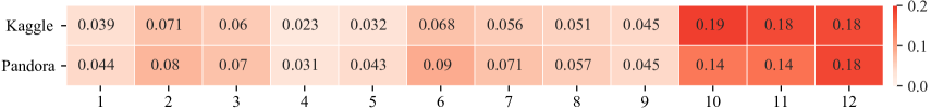
Figure 4: Visualization of layer attention weights. The last three layers supply with more information for this task.

5.2 Ablation Study

We conduct an ablation study of our TrigNet model on the Kaggle dataset by removing each component to investigate their contributions. Table 3 shows the results which are categorized into two groups.

In the first group, we investigate the contributions of the network components. We can see that removing the flow “$p{\rm{\leftrightarrow}}w{\rm{\leftrightarrow}}c{\rm{\leftrightarrow}}w{\rm{\leftrightarrow}}p$” defined in Eq. (5) results in higher performance declines than removing the flow “$p{\rm{\leftrightarrow}}w{\rm{\leftrightarrow}}p$” defined in Eq. (4), implying that the category nodes are helpful to capture personality cues from the texts. Besides, removing the layer attention mechanism also leads to considerable performance degradation.

In the second group, we investigate the contribution of each category node. The results, sorted by scores of decrease from small to large, demonstrate that the introduction of every category node is beneficial to TrigNet. Among these category nodes, the Affect is shown to be the most crucial one to our model, as the average Macro-F1 score drops most significantly after it is removed. This implies that the Affect category reflects one’s personality obviously. Similar conclusions are reported by Depue and Collins (1999) and Zhang et al. (2019). In addition, the Function node is the least impactful category node. The reason could be that functional words reflect pure linguistic knowledge and are weakly connected to personality.

5.3 Analysis of the Computational Cost

In this work we propose a flow GAT to reduce the computational cost of vanilla GAT. To show its effect, we compare it with vanilla GAT (as illustrated in the left part of Figure 3). The results are reported in Table 4, from which we can observe that flow GAT successfully reduces the computational cost in FLOPS and Memory by 38% and 32%, respectively, without extra parameters introduced. Besides, flow GAT is superior to vanilla GAT when the number of layers is 1. The cause is that the former can already capture adequate interactions between nodes with one layer, while the latter has to stack four layers to achieve this.

We also compare our TrigNet with the vanilla BERT in terms of the computational cost. The result show that the flow GAT takes about 1.14% more FLOPS than the vanilla BERT(297.3G).

GAT	Params	FLOPS	Memory	Ave.F1
Original	1.8M	5.5G	7.8GB	69.69
Flow(our)	1.8M	3.4G	5.3GB	70.86

Table 4: Analysis of the computational cost for original GAT and flow GAT on the Kaggle dataset. The metrics include the number of parameters (Params) and floating-point operations per second (FLOPS) of GAT as well as memory size (Memory) and the average Macro-F1 (Ave.F1) of whole model on the Kaggle dataset.

5.4 Layer Attention Analysis

This study adopts layer attention Peters et al. (2018) as shown in Eq. (2) to produce initial embeddings for post nodes. To show which layers are more useful, we conduct a simple experiment on the two datasets by using all the 12 layer representations of BERT and visualize the attention weight of each layer. As plotted in Figure 4, we find that the attention weights from layers 10 to 12 are significantly greater than that of the rest layers on both datasets, which explains why the last three layers are chosen for layer attention in our model.

6 Conclusion

In this work, we proposed a novel psycholinguistic knowledge-based tripartite graph network, TrigNet, for personality detection. TrigNet aims to introduce structural psycholinguistic knowledge from LIWC via constructing a tripartite graph, in which interactions between posts are captured through psychologically relevant words and categories rather than simple document-word or sentence-word relations. Besides, a novel flow GAT that only transmits messages between neighboring parties was developed to reduce the computational cost. Extensive experiments and analyses on two datasets demonstrate the effectiveness and efficiency of TrigNet. This work is the first effort to leverage a tripartite graph to explicitly incorporate psycholinguistic knowledge for personality detection, providing a new perspective for exploiting domain knowledge.

Ethical Statement

This study aims to develop a technical method to incorporate psycholinguistic knowledge into neural models, rather than creating a privacy-invading tool. We worked within the purview of acceptable privacy practices and strictly followed the data usage policy. The datasets used in this study are all from public sources with all user information anonymized. The assessment results of the proposed model are sensitive and should be shared selectively and subject to the approval of the institutional review board (IRB). Any research or application based on this study is only allowed for research purposes, and any attempt to use the proposed model to infer sensitive user characteristics from publicly accessible data is strictly prohibited.

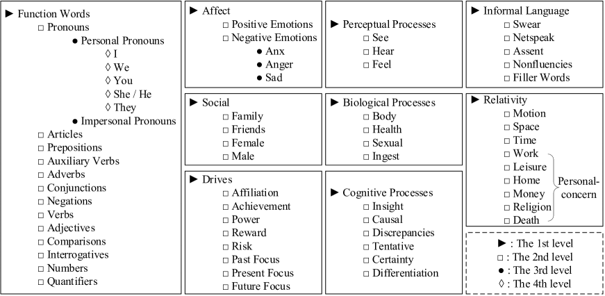
Figure 5: Detailed division of categories in the LIWC-2015 dictionary.

Appendix A Categories of LIWC

As shown in Figure 5, a total of 73 categories and subcategories are defined in the LIWC-2015 dictionary. There are 9 main categories: Function, Affect, Social, Cognitive Processes, Perceptual Processes, Biological Processes, Drives, Relativity, and Informal Language, in which 20 standard linguistic subcategories are included in the Function category and 44 psychological-relevant subcategories are defined in the rest 8 categories.

References

- Cao et al. (2019) Yu Cao, Meng Fang, and Dacheng Tao. 2019. Bag: Bi-directional attention entity graph convolutional network for multi-hop reasoning question answering. In Proceedings of the 2019 Conference of the North American Chapter of the Association for Computational Linguistics: Human Language Technologies, Volume 1 (Long and Short Papers), pages 357–362.
- Cho et al. (2014) Kyunghyun Cho, Bart van Merriënboer, Caglar Gulcehre, Dzmitry Bahdanau, Fethi Bougares, Holger Schwenk, and Yoshua Bengio. 2014. Learning phrase representations using rnn encoder–decoder for statistical machine translation. In Proceedings of the 2014 Conference on Empirical Methods in Natural Language Processing (EMNLP), pages 1724–1734.
- Cui and Qi (2017) Brandon Cui and Calvin Qi. 2017. Survey analysis of machine learning methods for natural language processing for mbti personality type prediction. Available online: http://cs229.stanford.edu/proj2017/final-reports/5242471.pdf (accessed on 26 May 2021).
- Depue and Collins (1999) Richard A Depue and Paul F Collins. 1999. Neurobiology of the structure of personality: Dopamine, facilitation of incentive motivation, and extraversion. Behavioral and Brain Sciences, 22(3):491–517.
- Devlin et al. (2019) Jacob Devlin, Ming-Wei Chang, Kenton Lee, and Kristina Toutanova. 2019. Bert: Pre-training of deep bidirectional transformers for language understanding. In Proceedings of the 2019 Conference of the North American Chapter of the Association for Computational Linguistics: Human Language Technologies, Volume 1 (Long and Short Papers), pages 4171–4186.
- Gjurković et al. (2020) Matej Gjurković, Mladen Karan, Iva Vukojević, Mihaela Bošnjak, and Jan Šnajder. 2020. Pandora talks: Personality and demographics on reddit. arXiv preprint arXiv:2004.04460.
- Golbeck et al. (2011) Jennifer Golbeck, Cristina Robles, and Karen Turner. 2011. Predicting personality with social media. In CHI’11 Extended Abstracts on Human Factors in Computing Systems, pages 253–262.
- Golbeck (2016) Jennifer Ann Golbeck. 2016. Predicting personality from social media text. AIS Transactions on Replication Research, 2(1):2.
- Goreis and Voracek (2019) Andreas Goreis and Martin Voracek. 2019. A systematic review and meta-analysis of psychological research on conspiracy beliefs: Field characteristics, measurement instruments, and associations with personality traits. Frontiers in Psychology, 10:205.
- Gottschalk (1997) Louis A Gottschalk. 1997. The unobtrusive measurement of psychological states and traits. Text Analysis for the Social Sciences: Methods for Drawing Statistical Inferences from Texts and Transcripts, pages 117–129.
- Hernandez and Knight (2017) R Hernandez and IS Knight. 2017. Predicting myers-bridge type indicator with text classification. In Proceedings of the 31st Conference on Neural Information Processing Systems, Long Beach, CA, USA, pages 4–9.
- Hiemstra et al. (2019) Annemarie MF Hiemstra, Janneke K Oostrom, Eva Derous, Alec W Serlie, and Marise Ph Born. 2019. Applicant perceptions of initial job candidate screening with asynchronous job interviews: Does personality matter? Journal of Personnel Psychology, 18(3):138.
- Hochreiter and Schmidhuber (1997) Sepp Hochreiter and Jürgen Schmidhuber. 1997. Long short-term memory. Neural Computation, 9(8):1735–1780.
- Jeong et al. (2020) Chi-Seo Jeong, Jong-Yong Lee, and Kye-Dong Jung. 2020. Adaptive recommendation system for tourism by personality type using deep learning. International Journal of Internet, Broadcasting and Communication, 12(1):55–60.
- Jiang et al. (2020) Hang Jiang, Xianzhe Zhang, and Jinho D Choi. 2020. Automatic text-based personality recognition on monologues and multiparty dialogues using attentive networks and contextual embeddings (student abstract). In Proceedings of the AAAI Conference on Artificial Intelligence, volume 34, pages 13821–13822.
- Keh et al. (2019) Sedrick Scott Keh, I Cheng, et al. 2019. Myers-briggs personality classification and personality-specific language generation using pre-trained language models. arXiv preprint arXiv:1907.06333.
- Kingma and Ba (2014) Diederik P Kingma and Jimmy Ba. 2014. Adam: A method for stochastic optimization. arXiv preprint arXiv:1412.6980.
- LeCun et al. (1998) Yann LeCun, Léon Bottou, Yoshua Bengio, and Patrick Haffner. 1998. Gradient-based learning applied to document recognition. Proceedings of the IEEE, 86(11):2278–2324.
- Liu et al. (2019) Yinhan Liu, Myle Ott, Naman Goyal, Jingfei Du, Mandar Joshi, Danqi Chen, Omer Levy, Mike Lewis, Luke Zettlemoyer, and Veselin Stoyanov. 2019. Roberta: A robustly optimized bert pretraining approach. arXiv preprint arXiv:1907.11692.
- Lynn et al. (2020) Veronica Lynn, Niranjan Balasubramanian, and H Andrew Schwartz. 2020. Hierarchical modeling for user personality prediction: The role of message-level attention. In Proceedings of the 58th Annual Meeting of the Association for Computational Linguistics, pages 5306–5316.
- Majumder et al. (2017) Navonil Majumder, Soujanya Poria, Alexander Gelbukh, and Erik Cambria. 2017. Deep learning-based document modeling for personality detection from text. IEEE Intelligent Systems, 32(2):74–79.
- Pennington et al. (2014) Jeffrey Pennington, Richard Socher, and Christopher D Manning. 2014. Glove: Global vectors for word representation. In Proceedings of the 2014 Conference on Empirical Methods in Natural Language Processing (EMNLP), pages 1532–1543.
- Peters et al. (2018) Matthew E Peters, Mark Neumann, Mohit Iyyer, Matt Gardner, Christopher Clark, Kenton Lee, and Luke Zettlemoyer. 2018. Deep contextualized word representations. In Proceedings of NAACL-HLT, pages 2227–2237.
- Sumner et al. (2012) Chris Sumner, Alison Byers, Rachel Boochever, and Gregory J Park. 2012. Predicting dark triad personality traits from twitter usage and a linguistic analysis of tweets. In 2012 11th International Conference on Machine Learning and Applications, volume 2, pages 386–393. IEEE.
- Szegedy et al. (2017) Christian Szegedy, Sergey Ioffe, Vincent Vanhoucke, and Alexander Alemi. 2017. Inception-v4, inception-resnet and the impact of residual connections on learning. In Proceedings of the AAAI Conference on Artificial Intelligence, volume 31.
- Tadesse et al. (2018) Michael M Tadesse, Hongfei Lin, Bo Xu, and Liang Yang. 2018. Personality predictions based on user behavior on the facebook social media platform. IEEE Access, 6:61959–61969.
- Tandera et al. (2017) Tommy Tandera, Derwin Suhartono, Rini Wongso, Yen Lina Prasetio, et al. 2017. Personality prediction system from facebook users. Procedia computer science, 116:604–611.
- Tausczik and Pennebaker (2010) Yla R Tausczik and James W Pennebaker. 2010. The psychological meaning of words: Liwc and computerized text analysis methods. Journal of Language and Social Psychology, 29(1):24–54.
- Vaswani et al. (2017) Ashish Vaswani, Noam Shazeer, Niki Parmar, Jakob Uszkoreit, Llion Jones, Aidan N Gomez, Łukasz Kaiser, and Illia Polosukhin. 2017. Attention is all you need. In Advances in Neural Information Processing Systems, pages 5998–6008.
- Veličković et al. (2018) Petar Veličković, Guillem Cucurull, Arantxa Casanova, Adriana Romero, Pietro Liò, and Yoshua Bengio. 2018. Graph attention networks. In International Conference on Learning Representations.
- Wang et al. (2020a) Danqing Wang, Pengfei Liu, Yining Zheng, Xipeng Qiu, and Xuanjing Huang. 2020a. Heterogeneous graph neural networks for extractive document summarization. In Proceedings of the 58th Annual Meeting of the Association for Computational Linguistics, pages 6209–6219.
- Wang et al. (2020b) Kai Wang, Weizhou Shen, Yunyi Yang, Xiaojun Quan, and Rui Wang. 2020b. Relational graph attention network for aspect-based sentiment analysis. In Proceedings of the 58th Annual Meeting of the Association for Computational Linguistics, pages 3229––3238.
- Wu et al. (2016) Yonghui Wu, Mike Schuster, Zhifeng Chen, Quoc V Le, Mohammad Norouzi, Wolfgang Macherey, Maxim Krikun, Yuan Cao, Qin Gao, Klaus Macherey, et al. 2016. Google’s neural machine translation system: Bridging the gap between human and machine translation. arXiv preprint arXiv:1609.08144.
- Xue et al. (2018) Di Xue, Lifa Wu, Zheng Hong, Shize Guo, Liang Gao, Zhiyong Wu, Xiaofeng Zhong, and Jianshan Sun. 2018. Deep learning-based personality recognition from text posts of online social networks. Applied Intelligence, 48(11):4232–4246.
- Yang and Huang (2019) Hsin-Chang Yang and Zi-Rui Huang. 2019. Mining personality traits from social messages for game recommender systems. Knowledge-Based Systems, 165:157–168.
- Yao et al. (2019) Liang Yao, Chengsheng Mao, and Yuan Luo. 2019. Graph convolutional networks for text classification. In Proceedings of the AAAI Conference on Artificial Intelligence, volume 33, pages 7370–7377.
- Zhang et al. (2019) Le Zhang, Songyou Peng, and Stefan Winkler. 2019. Persemon: A deep network for joint analysis of apparent personality, emotion and their relationship. IEEE Transactions on Affective Computing.
- Zhang et al. (2010) Yin Zhang, Rong Jin, and Zhi-Hua Zhou. 2010. Understanding bag-of-words model: a statistical framework. International Journal of Machine Learning and Cybernetics, 1(1-4):43–52.