Symmetric Spaces for Graph Embeddings: A Finsler-Riemannian Approach

Abstract

Learning faithful graph representations as sets of vertex embeddings has become a fundamental intermediary step in a wide range of machine learning applications. We propose the systematic use of symmetric spaces in representation learning, a class encompassing many of the previously used embedding targets. This enables us to introduce a new method, the use of Finsler metrics integrated in a Riemannian optimization scheme, that better adapts to dissimilar structures in the graph. We develop a tool to analyze the embeddings and infer structural properties of the data sets. For implementation, we choose Siegel spaces, a versatile family of symmetric spaces. Our approach outperforms competitive baselines for graph reconstruction tasks on various synthetic and real-world datasets. We further demonstrate its applicability on two downstream tasks, recommender systems and node classification.

1 Introduction

The goal of representation learning is to embed real-world data, frequently modeled on a graph, into an ambient space. This embedding space can then be used to analyze and perform tasks on the discrete graph. The predominant approach has been to embed discrete structures in an Euclidean space. Nonetheless, data in many domains exhibit non-Euclidean features (Krioukov et al., 2010; Bronstein et al., 2017), making embeddings into Riemannian manifolds with a richer structure necessary. For this reason, embeddings into hyperbolic (Krioukov et al., 2009; Nickel & Kiela, 2017; Sala et al., 2018; López & Strube, 2020) and spherical spaces (Wilson et al., 2014; Liu et al., 2017; Xu & Durrett, 2018) have been developed. Recent work proposes to combine different curvatures through several layers (Chami et al., 2019; Bachmann et al., 2020; Grattarola et al., 2020), to enrich the geometry by considering Cartesian products of spaces (Gu et al., 2019; Tifrea et al., 2019; Skopek et al., 2020), or to use Grassmannian manifolds or the space of symmetric positive definite matrices (SPD) as a trade-off between the representation capability and the computational tractability of the space (Huang & Gool, 2017; Huang et al., 2018; Cruceru et al., 2020). A unified framework in which to encompass these various examples is still missing.

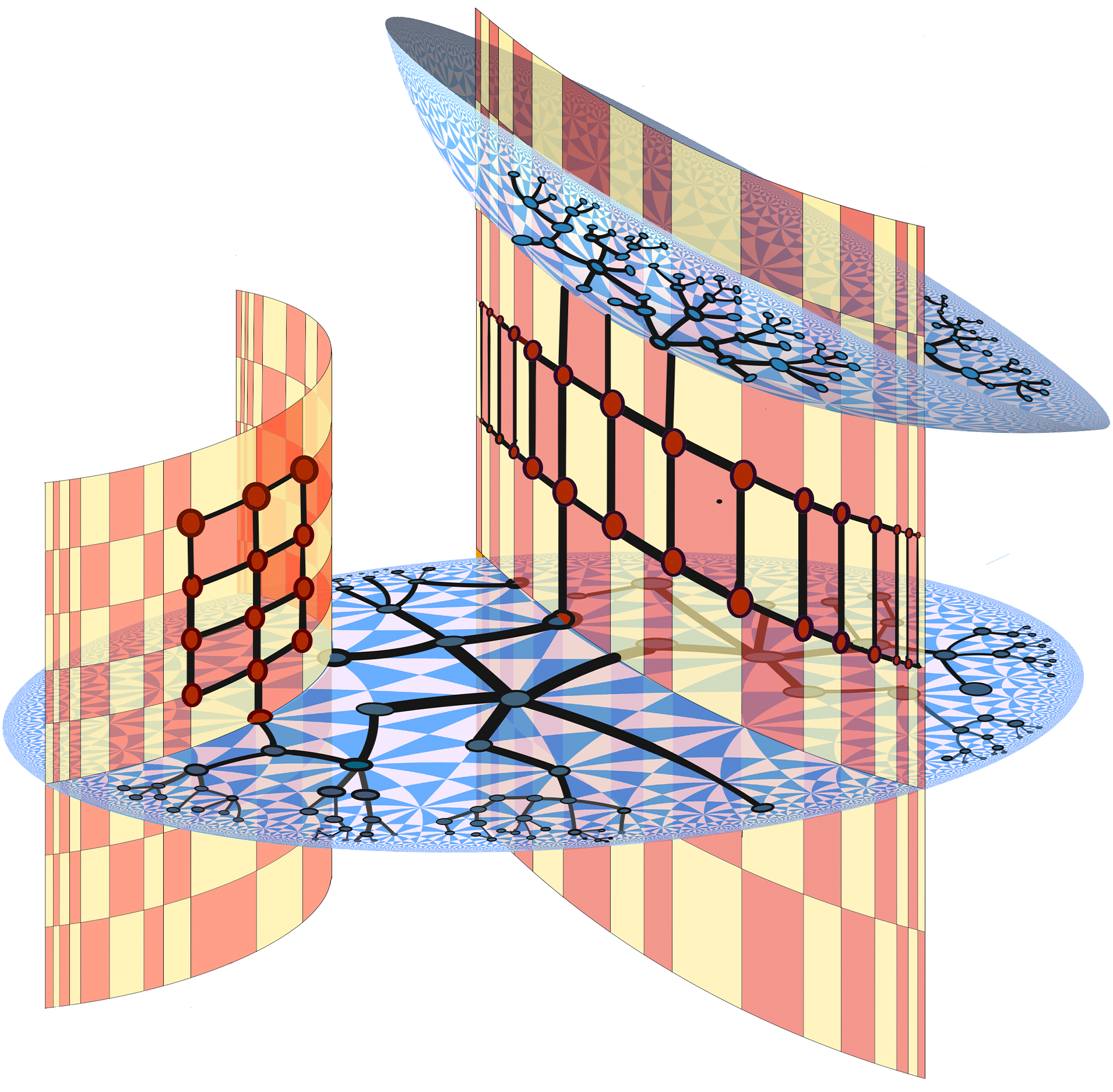
Figure 1: Symmetric spaces have a rich structure of totally geodesic subspaces, including flat subspaces (orange) and hyperbolic planes (blue). This compound, yet computationally tractable geometry allows isometric embeddings of many graphs, including those with subgraphs of dissimilar geometry. For example the graph embedded in the picture has both trees and grids as subgraphs.

In this work, we propose the systematic use of symmetric spaces in representation learning: this is a class comprising all the aforementioned spaces. Symmetric spaces are Riemannian manifolds with rich symmetry groups which makes them algorithmically tractable. They have a compound geometry that simultaneously contains Euclidean as well as hyperbolic or spherical subspaces, allowing them to automatically adapt to dissimilar features in the graph. We develop a general framework to choose a Riemannian symmetric space and implement the mathematical tools required to learn graph embeddings (§2). Our systematic view enables us to introduce the use of Finsler metrics integrated with a Riemannian optimization scheme as a new method to achieve graph representations. Moreover, we use a vector-valued distance function on symmetric spaces to develop a new tool for the analysis of the structural properties of the embedded graphs.

To demonstrate a concrete implementation of our general framework, we choose Siegel spaces (Siegel, 1943); a family of symmetric spaces that has not been explored in geometric deep learning, despite them being among the most versatile symmetric spaces of non-positive curvature. Key features of Siegel spaces are that they are matrix versions of the hyperbolic plane, they contain many products of hyperbolic planes as well as copies of SPD as submanifolds, and they support Finsler metrics that induce the $\ell^{1}$ or the $\ell^{\infty}$ metric on the Euclidean subspaces. As we verify in experiments, these metrics are well suited to embed graphs of mixed geometric features. This makes Siegel spaces with Finsler metrics an excellent device for embedding complex networks without a priori knowledge of their internal structure.

Siegel spaces are realized as spaces of symmetric matrices with coefficients in the complex numbers $\mathbb{C}$. By combining their explicit models and the general structure theory of symmetric spaces with the Takagi factorization (Takagi, 1924) and the Cayley transform (Cayley, 1846), we achieve a tractable and automatic-differentiable algorithm to compute distances in Siegel spaces (§4). This allows us to learn embeddings through Riemannian optimization (Bonnabel, 2011), which is easily parallelizable and scales to large datasets. Moreover, we highlight the properties of the Finsler metrics on these spaces (§3) and integrate them with the Riemannian optimization tools.

We evaluate the representation capacities of the Siegel spaces for the task of graph reconstruction on real and synthetic datasets. We find that Siegel spaces endowed with Finsler metrics outperform Euclidean, hyperbolic, Cartesian products of these spaces and SPD in all analyzed datasets. These results manifest the effectiveness and versatility of the proposed approach, particularly for graphs with varying and intricate structures.

To showcase potential applications of our approach in different graph embedding pipelines, we also test its capabilities for recommender systems and node classification. We find that our models surpass competitive baselines (constant-curvature, products thereof and SPD) for several real-world datasets.

Related Work: Riemannian manifold learning has regained attention due to appealing geometric properties that allow methods to represent non-Euclidean data arising in several domains (Rubin-Delanchy, 2020). Our systematic approach to symmetric spaces comprises embeddings in hyperbolic spaces (Chamberlain et al., 2017; Ganea et al., 2018; Nickel & Kiela, 2018; López et al., 2019), spherical spaces (Meng et al., 2019; Defferrard et al., 2020), combinations thereof (Bachmann et al., 2020; Grattarola et al., 2020; Law & Stam, 2020), Cartesian products of spaces (Gu et al., 2019; Tifrea et al., 2019), Grassmannian manifolds (Huang et al., 2018) and the space of symmetric positive definite matrices (SPD) (Huang & Gool, 2017; Cruceru et al., 2020), among others. We implement our method on Siegel spaces. To the best of our knowledge, we are the first work to apply them in Geometric Deep Learning.

Our general view allows us to to endow Riemannian symmetric spaces with Finsler metrics, which have been applied in compressed sensing (Donoho & Tsaig, 2008), for clustering categorical distributions (Nielsen & Sun, 2019), and in robotics (Ratliff et al., 2020). We provide strong experimental evidence that supports the intuition on how they offer a less distorted representation than Euclidean metrics for graphs with different structure. With regard to optimization, we derive the explicit formulations to employ a generalization of stochastic gradient descent (Bonnabel, 2011) as a Riemannian adaptive optimization method (Bécigneul & Ganea, 2019).

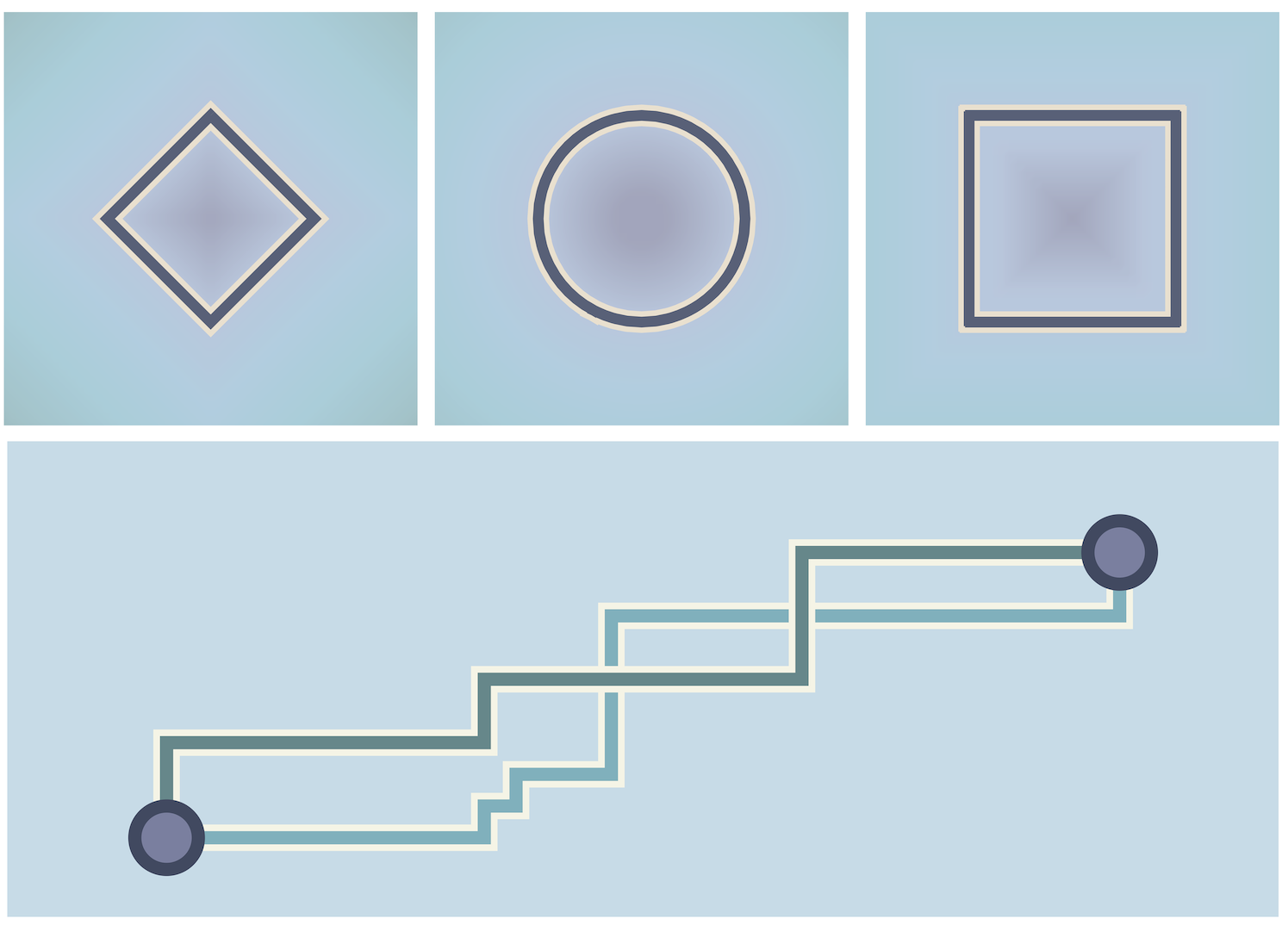
Figure 2: Above, from left to right: the unit spheres for the $\ell^{1}$, $\ell^{2}$ (Euclidean), and $\ell^{\infty}$ metrics on the plane. Below: Distance minimizing geodesics are not necessarily unique in Finsler geometry. The two paths shown have the same (minimal) $\ell^{1}$ length.

2 Symmetric Spaces for Embedding Problems

Riemannian symmetric spaces (RSS) are Riemannian manifolds with large symmetry groups, which makes them amenable to analytical tools as well as to explicit computations. A key feature of (non-compact) RSS is that they offer a rich combination of geometric features, including many subspaces isometric to Euclidean, hyperbolic spaces and products thereof. This makes them an excellent target tool for learning embeddings of complex networks without a priori knowledge of their internal structure.

First, we introduce two aspects of the general theory of RSS to representation learning: Finsler distances and vector-valued distances. These give us, respectively, a concrete method to obtain better graph representations, and a new tool to analyze graph embeddings. Then, we describe our general implementation framework for RSS.

Finsler Distances: Riemannian metrics are not well adapted to represent graphs. For example, though a two dimensional grid intuitively looks like a plane, any embedding of it in the Euclidean plane $\mathbb{R}^{2}$ necessarily distorts some distances by a factor of at least $\sqrt{2}$. This is due to the fact that while in the Euclidean plane length minimizing paths (geodesics) are unique, in graphs there are generally several shortest paths (see Figure 2). Instead, it is possible to find an abstract isometric embedding of the grid in $\mathbb{R}^{2}$ if the latter is endowed with the $\ell^{1}$ (or taxicab) metric. This is a first example of a Finsler distance. Another Finsler distance on $\mathbb{R}^{n}$ that plays a role in our work is the $\ell^{\infty}$ metric. See Appendix A.4 for a brief introduction.

RSS do not only support a Riemannian metric, but a whole family of Finsler distances with the same symmetry group (group of isometries). For the reasons explained above, these Finsler metrics are more suitable to embed complex networks. We verify these assumptions through concrete experiments in Section 5. Since Finsler metrics are in general not convex, they are less suitable for optimization problems. Due to this, we propose to combine the Riemannian and Finsler structure, by using a Riemannian optimization scheme, with loss functions based on the Finsler metric.

Vector-valued Distance: In Euclidean space, in the sphere or in hyperbolic space, the only invariant of two points is their distance. A pair of points can be mapped to any other pair of points iff their distance is the same. Instead, in a general RSS the invariant between two points is a distance vector in $\mathbb{R}^{n}$, where $n$ is the rank of the RSS. This is, two pairs of points can be separated by the same distance, but have different distance vectors. This vector-valued distance gives us a new tool to analyze graph embeddings, as we illustrate in Section 6.

The dimension of the space in which the vector-valued distance takes values in defines the rank of the RSS. Geometrically, this represents the largest Euclidean subspace which can be isometrically embedded (hence, hyperbolic and spherical spaces are of $\operatorname{rank}-1$). The symmetries of an RSS fixing such a maximal flat form a finite group — the Weyl group of the RSS. In the example of Siegel spaces discussed below, the Weyl group acts by permutations and reflections of the coordinates, allowing us to canonically represent each vector-valued distance as an $n$-tuple of non-increasing positive numbers. Such a uniform choice of standard representative for all vector-valued distances is a fundamental domain for this group action, known as a Weyl chamber for the RSS.

Implementation Schema: The general theory of RSS not only unifies many spaces previously applied in representation learning, but also systematises their implementation. Using standard tools of this theory, we provide a general framework to implement the mathematical methods required to learn graph embeddings in a given RSS.

Step 1, choosing an RSS: We may utilize the classical theory of symmetric spaces to inform our choice of RSS. Every symmetric space $M$ can be decomposed into an (almost) product $M=M_{1}\times\cdots\times M_{k}$ of irreducible symmetric spaces. Apart from twelve exceptional examples, there are eleven infinite families irreducible symmetric spaces — see Helgason (1978) for more details, or Appendix A, Table 6. Each family of irreducible symmetric space has a distinct family of symmetry groups, which in turn determines many mathematical properties of interest (for instance, the symmetry group determines the shape of the Weyl chambers, which determines the admissible Finsler metrics). Given a geometric property of interest, the theory of RSS allows one to determine which (if any) symmetric spaces enjoy it. For example, we choose Siegel spaces also because they admit Finsler metrics induced by the $\ell^{1}$ metric on flats, which agrees with the intrinsic metric on grid-like graphs.

Toolkit 1 Computing Distances

1:  Input from Model: Choice of basepoint $m$, maximal flat $F$, identification $\phi\colon F\to\mathbb{R}^{n}$, choice of Weyl Chamber $C\subset\mathbb{R}^{n}$, and Finsler norm $\|\cdot\|_{F}$ on $\mathbb{R}^{n}$.

2:  Given $p,q\in M$:

3:  Compute $g\in G$ such that $g(p)=m$ and $g(q)\in F$.

4:  Compute $v^{\prime}=\phi(g(q))\in\mathbb{R}^{n}$, and $h\in G$ the Weyl group element such that $h(v^{\prime})=v\in C$.

5:  The Vector-valued Distance (VVD) is $\mathrm{vDist}(p,q)=v$.

6:  The Riemannian Distance (RD) is $d^{R}(p,q)=\sqrt{\sum_{i}v_{i}^{2}}.$

7:  The Finsler Distance (FD) is $d^{F}(p,q)=\|v\|_{F}.$

8:  For a product $\prod M_{i}$, the VVD is the vector $\left(\mathrm{vDist}(p_{i},q_{i})\right)$ of VVDs for each $M_{i}$. The RD, FD satisfy the pythagorean theorem: $d^{X}(p,q)^{2}=\sum_{i}d^{X_{i}}(p_{i},q_{i})^{2}$, for $X\in\{R,F\}$.

Step 2, choosing a model of the RSS: Having selected an RSS, we must also select a model: a space $M$ representing its points equipped with an action of its symmetry group $G$. Such a choice is of practical, rather than theoretical concern: the points of $M$ should be easy to work with, and the symmetries of $G$ straightforward to compute and apply. Each RSS may have many already-understood models in the literature to select from. In our example of Siegel spaces, we implement two distinct models, selected because both their points and symmetries may be encoded by $n\times n$ matrices. See Section 3.

Implementing a product of symmetric spaces requires implementing each factor simultaneously. Given models $M_{1},\ldots,M_{k}$ with symmetry groups $G_{1},\ldots G_{k}$, the product $M=M_{1}\times\cdots\times M_{k}$ has as its points $m=(m_{1},\ldots,m_{k})$ the $k-$tuples with $m_{i}\in M_{i}$, with the group $G=G_{1}\times\cdots\times G_{k}$ acting componentwise. This general implementation of products directly generalizes products of constant curvature spaces.

Step 3, computing distances: Given a choice of RSS, the fundamental quantity to compute is a distance function on $M$, typically used in the loss function. In contrast to general Riemannian manifolds, the rich symmetry of RSS allows this computation to be factored into a sequence of geometric steps. See Toolkit 1 for a schematic implementation using data from the standard theory of RSS (choice of maximal flat, Weyl chamber, and Finsler norm) and Algorithm 1 for a concrete implementation in the Siegel spaces.

Step 4, computing gradients: To perform gradient-based optimization, the Riemannian gradient of these distance functions is required. Depending on the Riemannian optimization methods used, additional local geometry including parallel transport and the exponential map may be useful (Bonnabel, 2011; Bécigneul & Ganea, 2019). See Toolkit 2 for the relationships of these components to elements of the classical theory of RSS.

Toolkit 2 Computing Local Geometry

1:  Input From Model: Geodesic reflections $\sigma_{p}\in G$, the metric tensor $\langle\cdot,\cdot\rangle$, basepoint $m\in M$, orthogonal decomposition $\mathfrak{stab}(m)\oplus\mathfrak{p}=\mathfrak{g}$, and identification $\phi\colon T_{m}M\to\mathfrak{p}.$

2:  Given $f\colon M\to\mathbb{R}$, a geodesic $\gamma$, or $v\in T_{m}M$ respectively:

3:  The Riemannian Gradient of $f$ is computed from the metric tensor by solving $\langle{\rm grad}_{R}(f),-\rangle=df(-)$

4:  Parallel Transport along $\gamma$ is achieved by the differentials $(d\tau_{t})_{\gamma(t_{0})}$ of transvections $\tau_{t}=\sigma_{\gamma(t/2)}\sigma_{\gamma(t_{0})}$ along $\gamma$.

5:  The Riemannian Exponential $\exp_{m}^{R}(v)=g(m)$ is the matrix exponential $g=\exp(\phi(v))\in G$ applied to $m$.

6:  For a product $\prod M_{i}$ the Riemannian gradient, Parallel Transport, and Exponential map are computed component-wise.

See Appendix A and B for a review of the general theory relevant to this schema, and for an explicit implementation in the Siegel spaces.

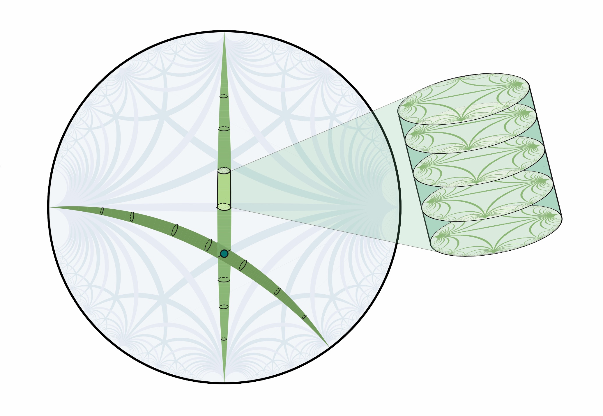
(a) Bounded Domain Model $\mathcal{B}_{n}$

(b) Siegel Upper Half Space $\mathcal{S}_{n}$

Figure 3: a) Every point of the disk is a complex symmetric $n$-dimensional matrix. b) A hyperbolic plane over SPD. $\mathcal{S}_{2}$ is a 6 dimensional manifold, the green lines represent totally geodesic submanifolds isometric to SPD that intersect in exactly one point. In dimension 2, SPD is isometric to the product of a hyperbolic plane and the line

3 Siegel Space

We implement the general aspects of the theory of RSS outlined above in the Siegel spaces HypSPD_n (Siegel, 1943), a versatile family of non-compact RSS, which has not yet been explored in geometric deep learning. The simplicity and the versatility of the Siegel space make it particularly suited for representation learning. We highlight some of its main features.

Models: HypSPD_n admits concrete and tractable matrix models generalizing the Poincaré disk and the upper half plane model of the hyperbolic space. Both are open subsets of the space ${\rm Sym}(n,\mathbb{C})$ of symmetric $n\times n$-matrices over $\mathbb{C}$. HypSPD_n has $n(n+1)$ dimensions.

The bounded symmetric domain model for HypSPD_n generalizes the Poincaré disk. It is given by:

$$\mathcal{B}_{n}:=\{Z\in{\rm Sym}(n,\mathbb{C})|\;{\rm Id}-Z^{*}Z>\!\!>0\};\vspace{0mm}$$ (1)

The Siegel upper half space model for HypSPD_n generalizes the upper half plane model of the hyperbolic plane by:

$$\mathcal{S}_{n}:=\{Z=X+iY\in{\rm Sym}(n,\mathbb{C})|\;Y>\!\!>0\}.\vspace{0mm}$$ (2)

An explicit isomorphism from $\mathcal{B}_{n}$ to $\mathcal{S}_{n}$ is given by the Cayley transform, a matrix analogue of the familiar map from the Poincare disk to upper half space model of the hyperbolic plane:

$$Z\mapsto i(Z+{\rm Id})(Z-{\rm Id})^{-1}.$$

Hyperbolic Plane over SPD: The Siegel space HypSPD_n contains SPD_n as a totally geodesic submanifold, and in fact, it can be considered as a hyperbolic plane over SPD. The role that real lines play in the hyperbolic plane, in HypSPD_n is played by SPD_n. This is illustrated in Figure 3b.

Totally Geodesic Subspaces: The Siegel space HypSPD_n contains $n$-dimensional Euclidean subspaces, products of $n$-copies of hyperbolic planes, SPD_n as well as products of Euclidean and hyperbolic spaces as totally geodesic subspaces (see Figure 3). It thus has a richer pattern of submanifolds than, for example, SPD. In particular, HypSPD_n contains more products of hyperbolic planes than SPD_n: in HypSPD_n we need 6 real dimension to contain $\mathbb{H}^{2}\times\mathbb{H}^{2}$ and 12 real dimension to contain $(\mathbb{H}^{2})^{3}$, whereas in SPD_n we would need 9 (resp. 20) dimensions for this.

Finsler Metrics: The Siegel space supports a Finsler metric $F_{1}$ that induces the $\ell^{1}$ metric on the Euclidean subspaces. As already remarked, the $\ell^{1}$ metric is particularly suitable for representing product graphs, or graphs that contain product subgraphs. Among all possible Finsler metrics supported by HypSPD_n, we focus on $F_{1}$ and $F_{\infty}$ (the latter induces the $\ell^{\infty}$ metric on the flat).

Scalability: Like all RSS, HypSPD_n has a dual – an RSS with similar mathematical properties but reversed curvature – generalizing the duality of $\mathbb{H}^{2}$ and $\mathbb{S}^{2}$. We focus on HypSPD_n over its dual for scalability reasons. The dual is a nonnegatively curved RSS of finite diameter, and thus does not admit isometric embeddings of arbitrarily large graphs. HypSPD_n, being nonpositively curved and infinite diameter, does not suffer from this restriction. See Appendix B.10 for details on its implementation and experiments with the dual.

4 Implementation

A complex number $z\in\mathbb{C}$ can be written as $z=x+iy$ where $x,y\in\mathbb{R}$ and $i^{2}=-1$. Analogously a complex symmetric matrix $Z\in{\rm Sym}(n,\mathbb{C})$ can be written as $Z=X+iY$, where $X=\Re(Z),Y=\Im(Z)\in{\rm Sym}(n,\mathbb{R})$ are symmetric matrices with real entries. We denote by $Z^{*}=X-iY$ the complex conjugate matrix.

Algorithm 1 Computing Distances

1:  Given two points $Z_{1},Z_{2}\in\mathcal{S}_{n}$:

2:  Define $Z_{3}=\sqrt{\Im(Z_{1})}^{-1}(Z_{2}-\Re(Z_{1}))\sqrt{\Im(Z_{1})}^{-1}\in\mathcal{S}_{n}$

3:  Define $W=(Z_{3}-i{\rm Id})(Z_{3}+i{\rm Id})^{-1}\in\mathcal{B}_{n}$

4:  Use the Takagi factorization to write $W=\overline{K}DK^{*}$ for $D$ real diagonal, and $K$ unitary.

5:  Define $v_{i}=\log\frac{1+d_{i}}{1-d_{i}}$ for $d_{i}$ the diagonal entries of $D$.

6:  Order the $v_{i}$ so that $v_{1}\geq v_{2}\geq\cdots\geq 0$. The Vector-valued Distance is $\mathrm{vDist}(Z_{1},Z_{2})=(v_{1},v_{2},\ldots,v_{n})$.

7:  The Riemannian distance is $d^{R}(Z_{1},Z_{2}):=\sqrt{\sum_{i=1}^{n}v_{i}^{2}}$.

8:  The Finsler distance inducing the $\ell^{1}$-metric is $d^{F1}(Z_{1},Z_{2}):=\sum_{i=1}^{n}v_{i}.$

9:  The Finsler distance inducing the $\ell^{\infty}$-metric is $d^{F\infty}(Z_{1},Z_{2}):=\max\{v_{i}\}=v_{1}$.

Distance Functions: To compute distances we apply either Riemannian or Finsler distance functions to the vector-valued distance. These computations are described in Algorithm 1, which is a concrete implementation of Toolkit 1. Specifically, step 2 moves one point to the basepoint, step 4 moves the other into our chosen flat, step 5 identifies this with $\mathbb{R}^{n}$ and step 6 returns the vector-valued distance, from which all distances are computed. We employ the Takagi factorization to obtain eigenvalues and eigenvectors of complex symmetric matrices in a tractable manner with automatic differentiation tools (see Appendix B.2).

Complexity of Distance Algorithm: Calculating distance between two points $Z_{1},Z_{2}$ in either $\mathcal{S}_{n}$ or $\mathcal{B}_{n}$ spaces implies computing multiplications, inversions and diagonalizations of $n\times n$ matrices. We find that the cost of the distance computation with respect to the matrix dimensions is $\mathcal{O}(n^{3})$. We prove this in Appendix D.

Riemannian Optimization with Finsler Distances: With the proposed matrix models of the Siegel space, we optimize objectives based on the Riemannian or Finsler distance functions in the embeddings space. To overcome the lack of convexity of Finsler metrics, we combine the Riemannian and the Finsler structure, by using a Riemannian optimization scheme (Bonnabel, 2011) with a loss function based on the Finsler metric. In Algorithm 2 we provide a way to compute the Riemannian gradient from the Euclidean gradient obtained via automatic differentiation. This is a direct implementation of Toolkit 2 Item 3.

To constrain the embeddings to remain within the Siegel space, we utilize a projection from the ambient space to our model. More precisely, given $\epsilon$ and a point $Z\in{\rm Sym}(n,\mathbb{C})$, we compute a point $Z_{\epsilon}^{\mathcal{S}}$ (resp. $Z_{\epsilon}^{\mathcal{B}}$) close to the original point lying in the $\epsilon$-interior of the model. For $\mathcal{S}_{n}$, starting from $Z=X+iY$ we orthogonally diagonalize $Y=K^{t}DK$, and then modify $D=\operatorname{diag}(d_{i})$ by setting each diagonal entry to $\max\{d_{i},\epsilon\}$. An analogous projection is defined on the bounded domain $\mathcal{B}_{n}$, see Appendix B.8.

Algorithm 2 Computing Riemannian Gradient

1:  Given $f:\mathcal{S}_{n}\to\mathbb{R}$ and $Z=X+iY\in\mathcal{S}_{n}$:

2:  Compute the Euclidean gradient ${\rm grad}_{E}(f)$ at $Z$ of $f$ obtained via automatic differentiation (see Appendix B.6).

3:  The Riemannian gradient is ${\rm grad_{R}}(f)=Y\cdot{\rm grad_{E}}(f)\cdot Y$.

4D Grid Tree Tree $\times$ Grid Tree $\times$ Tree Tree $\diamond$ Grids Grid $\diamond$ Trees $(|V|,|E|)$ $(625,2000)$ $(364,363)$ $(496,1224)$ $(225,420)$ $(775,1270)$ $(775,790)$ $D_{avg}$ mAP $D_{avg}$ mAP $D_{avg}$ mAP $D_{avg}$ mAP $D_{avg}$ mAP $D_{avg}$ mAP $\mathbb{E}^{20}$ 11.24$\pm$0.00 100.00 3.92$\pm$0.04 42.30 9.81$\pm$0.00 83.32 9.78$\pm$0.00 96.03 3.86$\pm$0.02 34.21 4.28$\pm$0.04 27.50 $\mathbb{H}^{20}$ 25.23$\pm$0.05 63.74 0.54$\pm$0.02 100.00 17.21$\pm$0.21 83.16 20.59$\pm$0.11 75.67 14.56$\pm$0.27 44.14 14.62$\pm$0.13 30.28 $\mathbb{E}^{10}\times\mathbb{H}^{10}$ 11.24$\pm$0.00 100.00 1.19$\pm$0.04 100.00 9.20$\pm$0.01 100.00 9.30$\pm$0.04 98.03 2.15$\pm$0.05 58.23 2.03$\pm$0.01 97.88 $\mathbb{H}^{10}\times\mathbb{H}^{10}$ 18.74$\pm$0.01 78.47 0.65$\pm$0.02 100.00 13.02$\pm$0.91 88.01 8.61$\pm$0.03 97.63 1.08$\pm$0.06 77.20 2.80$\pm$0.65 84.88 $\operatorname{SPD}_{6}$ 11.24$\pm$0.00 100.00 1.79$\pm$0.02 55.92 9.23$\pm$0.01 99.73 8.83$\pm$0.01 98.49 1.56$\pm$0.02 62.31 1.83$\pm$0.00 72.17 $\mathcal{S}_{4}^{R}$ 11.27$\pm$0.01 100.00 1.35$\pm$0.02 78.53 9.13$\pm$0.01 99.92 8.68$\pm$0.02 98.03 1.45$\pm$0.09 72.49 1.54$\pm$0.08 76.66 $\mathcal{S}_{4}^{F_{\infty}}$ 5.92$\pm$0.06 99.61 1.23$\pm$0.28 99.56 4.81$\pm$0.55 99.28 3.31$\pm$0.06 99.95 10.88$\pm$0.19 63.52 10.48$\pm$0.21 72.53 $\mathcal{S}_{4}^{F_{1}}$ 0.01$\pm$0.00 100.00 0.76$\pm$0.02 91.57 0.81$\pm$0.08 100.00 1.08$\pm$0.16 100.00 1.03$\pm$0.00 78.71 0.84$\pm$0.06 80.52 $\mathcal{B}_{4}^{R}$ 11.28$\pm$0.01 100.00 1.27$\pm$0.05 74.77 9.24$\pm$0.13 99.22 8.74$\pm$0.09 98.12 2.88$\pm$0.32 72.55 2.76$\pm$0.11 96.29 $\mathcal{B}_{4}^{F_{\infty}}$ 7.32$\pm$0.16 97.92 1.51$\pm$0.13 99.73 8.70$\pm$0.87 96.40 4.26$\pm$0.26 99.70 6.55$\pm$1.77 73.80 7.15$\pm$0.85 90.51 $\mathcal{B}_{4}^{F_{1}}$ 0.39$\pm$0.02 100.00 0.77$\pm$0.02 94.64 0.90$\pm$0.08 100.00 1.28$\pm$0.16 100.00 1.09$\pm$0.03 76.55 0.99$\pm$0.01 81.82

Table 1: Results for synthetic datasets. Lower $D_{avg}$ is better. Higher mAP is better. Metrics are given as percentage.

5 Graph Reconstruction

We evaluate the representation capabilities of the proposed approach for the task of graph reconstruction.

Setup: We embed graph nodes in a transductive setting. As input and evaluation data we take the shortest distance in the graph between every pair of connected nodes. Unlike previous work (Gu et al., 2019; Cruceru et al., 2020) we do not apply any scaling, neither in the input graph distances nor in the distances calculated on the space. We experiment with the loss proposed in Gu et al. (2019), which minimizes the relation between the distance in the space, compared to the distance in the graph, and captures the average distortion. We initialize the matrix embeddings in the Siegel upper half space by adding small symmetric perturbations to the matrix basepoint $i{\rm Id}$. For the Bounded model, we additionally map the points with the Cayley transform (see Appendix B.7). In all cases we optimize with Rsgd (Bonnabel, 2011) and report the average of $5$ runs.

Baselines: We compare our approach to constant-curvature baselines, such as Euclidean ($\mathbb{E}$) and hyperbolic ($\mathbb{H}$) spaces (we compare to the Poincaré model (Nickel & Kiela, 2017) since the Bounded Domain model is a generalization of it), Cartesian products thereof ($\mathbb{E}\times\mathbb{H}$ and $\mathbb{H}\times\mathbb{H}$) (Gu et al., 2019), and symmetric positive definite matrices ($\operatorname{SPD}$) (Cruceru et al., 2020) in low and high dimensions. Preliminary experiments on the dual of HypSPD_n and on spherical spaces showed poor performance thus we do not compare to them (see Appendix B.12). To establish a fair comparison, each model has the same number of free parameters. This is, the spaces $\mathcal{S}_{n}$ and $\mathcal{B}_{n}$ have $n(n+1)$ parameters, thus we compare to baselines of the same dimensionality. All implementations are taken from Geoopt (Kochurov et al., 2020).

Metrics: Following previous work (Sala et al., 2018; Gu et al., 2019), we measure the quality of the learned embeddings by reporting average distortion $D_{avg}$, a global metric that considers the explicit value of all distances, and mean average precision mAP, a ranking-based measure for local neighborhoods (local metric) as fidelity measures.

Synthetic Graphs: As a first step, we investigate the representation capabilities of different geometric spaces on synthetic graphs. Previous work has focused on graphs with pure geometric features, such as grids, trees, or their Cartesian products (Gu et al., 2019; Cruceru et al., 2020), which mix the grid- and tree-like features globally. We expand our analysis to rooted products of trees and grids. These graphs mix features at different levels and scales. Thus, they reflect to a greater extent the complexity of intertwining and varying structure in different regions, making them a better approximation of real-world datasets. We consider the rooted product Tree $\diamond$ Grids of a tree and 2D grids, and Grid $\diamond$ Trees, of a 2D grid and trees. More experimental details, hyperparameters, formulas and statistics about the data are present in Appendix C.3.

We report the results for synthetic graphs in Table 1. We find that the Siegel space with Finsler metrics significantly outperform constant curvature baselines in all graphs, except for the tree, where they have competitive results with the hyperbolic models. We observe that Siegel spaces with the Riemannian metric perform on par with the matching geometric spaces or with the best-fitting product of spaces across graphs of pure geometry (grids and Cartesian products of graphs). However, the $F_{1}$ metric outperforms the Riemannian and $F_{\infty}$ metrics in all graphs, for both models. This is particularly noticeable for the 4D Grid, where the distortion achieved by $F_{1}$ models is almost null, matching the intuition of less distorted grid representations through the taxicab metric.

USCA312 bio-diseasome csphd EuroRoad Facebook $(|V|,|E|)$ $(312,48516)$ $(516,1188)$ $(1025,1043)$ $(1039,1305)$ $(4039,88234)$ $D_{avg}$ $D_{avg}$ mAP $D_{avg}$ mAP $D_{avg}$ mAP $D_{avg}$ mAP $\mathbb{E}^{20}$ 0.18$\pm$0.01 3.83$\pm$0.01 76.31 4.04$\pm$0.01 47.37 4.50$\pm$0.00 87.70 3.16$\pm$0.01 32.21 $\mathbb{H}^{20}$ 2.39$\pm$0.02 6.83$\pm$0.08 91.26 22.42$\pm$0.23 60.24 43.56$\pm$0.44 54.25 3.72$\pm$0.00 44.85 $\mathbb{E}^{10}\times\mathbb{H}^{10}$ 0.18$\pm$0.00 2.52$\pm$0.02 91.99 3.06$\pm$0.02 73.25 4.24$\pm$0.02 89.93 2.80$\pm$0.01 34.26 $\mathbb{H}^{10}\times\mathbb{H}^{10}$ 0.47$\pm$0.18 2.57$\pm$0.05 95.00 7.02$\pm$1.07 79.22 23.30$\pm$1.62 75.07 2.51$\pm$0.00 36.39 $\operatorname{SPD}_{6}$ 0.21$\pm$0.02 2.54$\pm$0.00 82.66 2.92$\pm$0.11 57.88 19.54$\pm$0.99 92.38 2.92$\pm$0.05 33.73 $\mathcal{S}_{4}^{R}$ 0.28$\pm$0.03 2.40$\pm$0.02 87.01 4.30$\pm$0.18 59.95 29.21$\pm$0.91 84.92 3.07$\pm$0.04 30.98 $\mathcal{S}_{4}^{F_{\infty}}$ 0.57$\pm$0.08 2.78$\pm$0.49 93.95 27.27$\pm$1.00 59.45 46.82$\pm$1.02 72.03 1.90$\pm$0.11 45.58 $\mathcal{S}_{4}^{F_{1}}$ 0.18$\pm$0.02 1.55$\pm$0.04 90.42 1.50$\pm$0.03 64.11 3.79$\pm$0.07 94.63 2.37$\pm$0.07 35.23 $\mathcal{B}_{4}^{R}$ 0.24$\pm$0.07 2.69$\pm$0.10 89.11 28.65$\pm$3.39 62.66 53.45$\pm$2.65 48.75 3.58$\pm$0.10 30.35 $\mathcal{B}_{4}^{F_{\infty}}$ 0.21$\pm$0.04 4.58$\pm$0.63 90.36 26.32$\pm$6.16 54.94 52.69$\pm$2.28 48.75 2.18$\pm$0.18 39.15 $\mathcal{B}_{4}^{F_{1}}$ 0.18$\pm$0.07 1.54$\pm$0.02 90.41 2.96$\pm$0.91 67.58 21.98$\pm$0.62 91.63 5.05$\pm$0.03 39.87

Table 2: Results for real-world datasets. Lower $D_{avg}$ is better. Higher mAP is better. Metrics are given as percentage.

Even when the structure of the data conforms to the geometry of baselines, the Siegel spaces with the Finsler-Riemannian approach are able to outperform them by automatically adapting to very dissimilar patterns without any a priori estimates of the curvature or other features of the graph. This showcases the flexibility of our models, due to its enhanced geometry and higher expressivity.

For graphs with mixed geometric features (rooted products), Cartesian products of spaces cannot arrange these compound geometries into separate Euclidean and hyperbolic subspaces. RSS, on the other hand, offer a less distorted representation of these tangled patterns by exploiting their richer geometry which mixes hyperbolic and Euclidean features. Moreover, they reach a competitive performance on the local neighborhood reconstruction, as the mean precision shows. Results for more dimensionalities are given in Appendix F.

Tree $\times$ Grid Grid $\diamond$ Trees bio-diseasome $D_{avg}$ mAP $D_{avg}$ mAP $D_{avg}$ mAP $\mathcal{S}_{4}^{R}$ 9.13 99.92 1.54 76.66 2.40 87.01 $\mathcal{S}_{4}^{F_{\infty}}$ 4.81 99.28 10.48 72.53 2.78 93.95 $\mathcal{S}_{4}^{F_{1}}$ 0.81 100.00 0.84 80.52 1.55 90.42 $\mathbb{E}^{306}$ 9.80 85.14 2.81 67.69 3.52 88.45 $\mathbb{H}^{306}$ 17.31 82.97 15.92 27.14 7.04 91.46 $\mathbb{S}^{306}$ 73.78 35.36 81.67 58.26 70.91 84.61 $\mathbb{E}^{153}\times\mathbb{H}^{153}$ 9.14 100.00 1.52 97.85 2.36 95.65 $\mathbb{S}^{153}\times\mathbb{S}^{153}$ 60.71 6.93 70.00 5.64 55.51 19.51 $\mathcal{S}_{17}^{R}$ 9.19 99.89 1.31 75.45 2.13 93.14 $\mathcal{S}_{17}^{F_{\infty}}$ 4.82 97.45 11.45 94.09 1.50 98.27 $\mathcal{S}_{17}^{F_{1}}$ 0.03 100.00 0.27 99.23 0.73 99.09

Table 3: Results for different datasets in high-dimensional spaces. Best result is bold, second best underlined.

Real-world Datasets: We compare the models on two road networks, namely USCA312 of distances between North American cities and EuroRoad between European cities, bio-diseasome, a network of human disorders and diseases with reference to their genetic origins (Goh et al., 2007), a graph of computer science Ph.D. advisor-advisee relationships (Nooy et al., 2011), and a dense social network from Facebook (McAuley & Leskovec, 2012). These graphs have been analyzed in previous work as well (Gu et al., 2019; Cruceru et al., 2020).

We report the results in Table 2. On the USCA312 dataset, which is the only weighted graph under consideration, the Siegel spaces perform on par with the compared target manifolds. For all other datasets, the model with Finsler metrics outperforms all baselines. In line with the results for synthetic datasets, the $F_{1}$ metric exhibits an outstanding performance across several datasets.

Overall, these results show the strong reconstruction capabilities of RSS for real-world data as well. It also indicates that vertices in these real-world dataset form networks with a more intricate geometry, which the Siegel space is able to unfold to a better extent.

High-dimensional Spaces: In Table 3 we compare the approach in high-dimensional spaces (rank $17$ which is equal to $306$ free parameters), also including spherical spaces $\mathbb{S}$. The results show that our models operate well with larger matrices, where we see further improvement in our distortion and mean average precision over the low dimensional spaces of rank $4$. We observe that even though we notably increase the dimensions of the baselines to $306$, the Siegel models of rank $4$ (equivalent to $20$ dimensions) significantly outperform them. These results match the expectation that the richer variable curvature geometry of RSS better adapts to graphs with intricate geometric structures.

6 Analysis of the Embedding Space

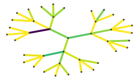
(a)

(b)

(c)

Figure 4: Edge coloring of $\mathcal{S}_{2}^{F1}$ for a tree (left), and a rooted product of tree $\diamond$ grids (center), and of grid $\diamond$ trees.

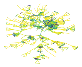
(a)

(b)

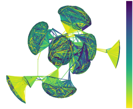
(c)

Figure 5: Edge coloring of $\mathcal{S}_{2}^{F1}$ for bio-diseasome (left) and csphd (center) and facebook (right). Edge colors indicate the angle of the vector-valued distance for each edge, on a linear scale from 0 (yellow) to $\pi/4$ (blue).

One reason to embed graphs into Riemannian manifolds is to use geometric properties of the manifold to analyze the structure of the graph. Embeddings into hyperbolic spaces, for example, have been used to infer and visualize hierarchical structure in data sets (Nickel & Kiela, 2018). Visualizations in RSS are difficult due to their high dimensionality. As a solution we use the vector-valued distance function in the RSS to develop a new tool to visualize and to analyze structural properties of the graphs.

We focus on HypSPD₂, the Siegel space of rank $k=2$, where the vector-valued distance is just a vector in a cone in $\mathbb{R}^{2}$. We take edges $(Z_{i},Z_{j})$ and assign the angle of the vector $\mathrm{vDist}(Z_{i},Z_{j})=(v_{1},v_{2})$ (see Algorithm 1, step $6$) to each edge in the graph. This angle assignment provides a continuous edge coloring that can be leveraged to find structure in graphs.

We see in Figure 4 that the edge coloring makes the large-scale structure of the tree (blue/green edges) and the leaves (yellow edges) visible. This is even more striking for the rooted products. In tree $\diamond$ grids the edge coloring distinguishes the hyperbolic parts of the graph (blue edges) and the Euclidean parts (yellow edges). For the grid $\diamond$ trees, the Euclidean parts are labelled by blue/green edges and the hyperbolic parts by yellow edges. Thus, even though we trained the embedding only on the metric, it automatically adapts to other features of the graph.

In the edge visualizations for real-world datasets (Figure 5), the edges in the denser connected parts of the graph have a higher angle, as it can be seen for the bio-diseasome and facebook data sets. For csphd, the tree structure is emphasized by the low angles.

This suggests that the continuous values that we assign to edges are a powerful tool to automatically discover dissimilar patterns in graphs. This can be further used in efficient clustering of the graph. In Appendix E we give similar visualizations for the Riemannian metric and the $F_{\infty}$ Finsler metric, showing that also with respect to exhibiting structural properties, the $F_{1}$ metric performs best.

7 Downstream Tasks

We also evaluate the representation capabilities of Siegel spaces on two downstream tasks: recommender systems and node classification.

7.1 Recommender Systems

Our method can be applied in downstream tasks that involve embedding graphs, such as recommender systems. These systems mine user-item interactions and recommend items to users according to the distance/similarity between their respective embeddings (Hsieh et al., 2017).

Setup: Given a set of observed user-item interactions $\mathcal{T}=\{(u,v)\}$, we follow a metric learning approach (Vinh Tran et al., 2020) and learn embeddings by optimizing the following hinge loss function:

$$\mathcal{L}=\sum_{(u,v)\in\mathcal{T}}\sum_{(u,w)\not\in\mathcal{T}}[m+d_{\mathbb{K}}(\textbf{u},\textbf{v})^{2}-d_{\mathbb{K}}(\textbf{u},\textbf{w})^{2}]_{+}$$ (3)

where $\mathbb{K}$ is the target space, $w$ is an item the user has not interacted with, $\textbf{u},\textbf{v},\textbf{w}\in\mathbb{K}$, $m>0$ is the hinge margin and $[z]_{+}=max(0,z)$. To generate recommendations, for each user $u$ we rank the items $\textbf{v}_{i}$ according to their distance to u. Since it is very costly to rank all the available items, we randomly select $100$ samples which the user has not interacted with, and rank the ground truth amongst these samples (He et al., 2017). We adopt normalized discounted cumulative gain (nDG) and hit ratio (HR), both at $10$, as ranking evaluation metrics for recommendations. More experimental details and data stats in Appendix C.4.

Data: We evaluate the different models over two MovieLens datasets (ml-1m and ml-100k) (Harper & Konstan, 2015), last.fm, a dataset of artist listening records (Cantador et al., 2011), and MeetUp, crawled from Meetup.com (Pham et al., 2015). To generate evaluation splits, the penultimate and last item the user has interacted with are withheld as dev and test set respectively.

Results: We report the performance for all analyzed models in Table 4. While in the Movies datasets, the Riemannian model marginally outperforms the baselines, in the other two cases the $F_{1}$ model achieves the highest performance by a larger difference. These systems learn to model users’ preferences, and embeds users and items in the space, in a way that is exploited for the task of generating recommendations. In this manner we demonstrate how downstream tasks can profit from the enhanced graph representation capacity of our models, and we highlight the flexibility of the method, in this case applied in combination with a collaborative metric learning approach (Hsieh et al., 2017).

ml-1m ml-100k lastfm MeetUp HR@10 nDG HR@10 nDG HR@10 nDG HR@10 nDG $\mathbb{E}^{20}$ 46.9$\pm$0.6 22.7 54.6$\pm$1.0 28.7 55.4$\pm$0.3 24.6 69.8$\pm$0.4 46.4 $\mathbb{H}^{20}$ 46.0$\pm$0.5 23.0 53.4$\pm$1.0 28.2 54.8$\pm$0.5 24.9 71.8$\pm$0.5 48.5 $\mathbb{E}^{10}\times\mathbb{H}^{10}$ 52.0$\pm$0.7 27.4 53.1$\pm$1.3 27.9 45.5$\pm$0.9 18.9 70.7$\pm$0.2 47.5 $\mathbb{H}^{10}\times\mathbb{H}^{10}$ 46.7$\pm$0.6 23.0 54.8$\pm$0.9 29.1 55.0$\pm$0.9 24.6 71.7$\pm$0.1 48.8 $\mathcal{SPD}_{6}$ 45.8$\pm$1.0 22.1 53.3$\pm$1.4 28.0 55.4$\pm$0.2 25.3 70.1$\pm$0.6 46.5 $\mathcal{S}_{4}^{R}$ 53.8$\pm$0.3 27.7 55.7$\pm$0.9 28.6 53.1$\pm$0.5 24.8 65.8$\pm$1.2 43.4 $\mathcal{S}_{4}^{F_{\infty}}$ 45.9$\pm$0.9 22.7 52.5$\pm$0.3 27.5 53.8$\pm$1.7 32.5 69.0$\pm$0.5 46.4 $\mathcal{S}_{4}^{F_{1}}$ 52.9$\pm$0.6 27.2 55.6$\pm$1.3 29.4 61.1$\pm$1.2 38.0 74.9$\pm$0.1 52.8

Table 4: Results for recommender system datasets.

7.2 Node Classification

Our proposed graph embeddings can be used in conjunction with standard machine learning pipelines, such as downstream classification. To demonstrate this, and following the procedure of Chami et al. (2020), we embed three hierarchical clustering datasets based on the cosine distance between their points, and then use the learned embeddings as input features for a Euclidean logistic regression model. Since the node embeddings lie in different metric spaces, we apply the corresponding logarithmic map to obtain a ”flat” representation before classifying. For the Siegel models of dimension $n$, we first map each complex matrix embedding $Z=X+iY$ to $[(Y+XY^{-1}X,XY^{-1}),(Y^{-1}X,Y^{-1})]\in{\rm SPD}_{2n}$, this is the natural realisation of HypSPD_n as a totally geodesic submanifold of ${\rm SPD}_{2n}$, and then we apply the LogEig map (Huang & Gool, 2017), which yields a representation in a flat space. More experimental details in Appendix C.5.

Dataset Iris Zoo Glass $\mathbb{E}^{20}$ 83.3$\pm$1.1 88.7$\pm$1.8 67.2$\pm$2.5 $\mathbb{H}^{20}$ 84.0$\pm$0.6 87.3$\pm$1.5 62.8$\pm$2.0 $\mathbb{E}^{10}\times\mathbb{H}^{10}$ 85.6$\pm$1.1 88.0$\pm$1.4 64.8$\pm$4.3 $\mathbb{H}^{10}\times\mathbb{H}^{10}$ 87.8$\pm$1.4 87.3$\pm$1.5 63.4$\pm$3.4 $\operatorname{SPD}_{6}$ 88.0$\pm$1.6 88.7$\pm$2.2 66.9$\pm$2.0 $\mathcal{S}_{4}^{R}$ 88.0$\pm$0.5 88.7$\pm$2.2 66.6$\pm$2.4 $\mathcal{S}_{4}^{F_{\infty}}$ 89.1$\pm$0.5 88.7$\pm$2.5 65.2$\pm$3.0 $\mathcal{S}_{4}^{F_{1}}$ 89.3$\pm$1.1 90.7$\pm$1.5 67.5$\pm$3.9 $\mathcal{B}_{4}^{R}$ 86.0$\pm$1.9 88.7$\pm$1.4 65.5$\pm$3.1 $\mathcal{B}_{4}^{F_{\infty}}$ 84.4$\pm$0.0 87.3$\pm$1.9 65.6$\pm$1.7 $\mathcal{B}_{4}^{F_{1}}$ 85.6$\pm$1.4 89.3$\pm$2.8 64.2$\pm$1.7

Table 5: Accuracy for node classification based on its embedding.

Results are presented in Table 5. In all cases we see that the embeddings learned by our models capture the structural properties of the dataset, so that a simple classifier can separate the nodes into different clusters. They offer the best performance in the three datasets. This suggests that embeddings in Siegel spaces learn meaningful representations that can be exploited into downstream tasks. Moreover, we showcase how to map these embeddings to ”flat” vectors; in this way they can be integrated with classical Euclidean network layers.

8 Conclusions & Future Work

Riemannian manifold learning has regained attention due to appealing geometric properties that allow methods to represent non-Euclidean data arising in several domains. We propose the systematic use of symmetric spaces to encompass previous work in representation learning, and develop a toolkit that allows practitioners to choose a Riemannian symmetric space and implement the mathematical tools required to learn graph embeddings. We introduce the use of Finsler metrics integrated with a Riemannian optimization scheme, which provide a significantly less distorted representation over several data sets. As a new tool to discover structure in the graph, we leverage the vector-valued distance function on a RSS. We implement these ideas on Siegel spaces, a rich class of RSS that had not been explored in geometric deep learning, and we develop tractable and mathematically sound algorithms to learn embeddings in these spaces through gradient-descent methods. We showcase the effectiveness of the proposed approach on conventional as well as new datasets for the graph reconstruction task, and in two downstream tasks. Our method ties or outperforms constant-curvature baselines without requiring any previous assumption on geometric features of the graphs. This shows the flexibility and enhanced representation capacity of Siegel spaces, as well as the versatility of our approach.

As future directions, we consider applying the vector-valued distance in clustering and structural analysis of graphs, and the development of deep neural network architectures adapted to the geometry of RSS, specifically Siegel spaces. A further interesting research direction is to use geometric transition between symmetric spaces to extend the approach demonstrated by curvature learning à la Gu et al. (2019). We plan to leverage the structure of the Siegel space of a hyperbolic plane over SPD to analyze medical imaging data, which is often given as symmetric positive definite matrices, see Pennec (2020).

Appendix A Symmetric Spaces: a Short Overview

Type Non-compact Compact ${\rm rk}_{\mathbb{R}}$ $\dim$ AI ${\rm SL}(n,\mathbb{R})/{\rm SO}(n,\mathbb{R})$ ${\rm SU}(n)/{\rm SO}(n)$ $n-1$ $\frac{(n-1)(n+2)}{2}$ A ${\rm SL}(n,\mathbb{C})/{\rm SU}(2)$ $({\rm SU}(n)\times{\rm SU}(n))/{\rm SU}(n)$ $n-1$ $(n+1)(n-1)$ BDI ${\rm SO}(p,q)/{\rm SO}(p)\times{\rm SO}(q)$ ${\rm SO}(p+q)/{\rm SO}(p)\times{\rm SO}(q)$ $\min\{p,q\}$ $pq$ AIII ${\rm SU}(p,q)/{\rm SU}(p)\times{\rm SU}(q)$ ${\rm SU}(p+q)/{\rm SU}(p)\times{\rm SU}(q)$ $\min\{p,q\}$ $2pq$ CI ${\rm Sp}(2n,\mathbb{R})/{\rm U}(n)$ ${\rm Sp}(2n)/{\rm U}(n)$ $n$ $2n(n+1)$ DIII ${\rm SO}^{*}(2n)/{\rm U}(n)$ ${\rm SO}(2n)/{\rm U}(n)$ $\lfloor\frac{n}{2}\rfloor$ $n(n-1)$ CII ${\rm Sp}(p,q)/{\rm Sp}(p)\times{\rm Sp}(q)$ ${\rm Sp}(p+q)/{\rm Sp}(p)\times{\rm Sp}(q)$ $\min\{p,q\}$ $4pq$ AII ${\rm SL}(n,\mathbb{H})/{\rm Sp}(n)$ ${\rm SU}(2n)/{\rm Sp}(n)$ $n-1$ $(n-1)(2n+1)$ D ${\rm SO}(2n,\mathbb{C})/{\rm SO}(2n)$ $({\rm SO}(2n)\times{\rm SO}(2n))/{\rm SO}(2n)$ $n$ $n(2n-1)$ B ${\rm SO}(2n+1,\mathbb{C})/{\rm SO}(2n+1)$ $({\rm SO}(2n+1)\times{\rm SO}(2n+1))/{\rm SO}(2n+1)$ $n$ $n(2n+1)$ C ${\rm Sp}(n,\mathbb{C})/{\rm Sp}(n)$ $({\rm Sp}(n)\times{\rm Sp}(n))/{\rm Sp}(n)$ $n$

Table 6: The classical symmetric spaces. Row CI represents the Siegel spaces and their compact duals.

Riemannian symmetric spaces have been extensively studied by mathematicians, and there are many ways to characterize them. They can be described as simply connected Riemannian manifolds, for which the curvature is covariantly constant, or Riemannian manifolds, for which the geodesic reflection in each point defines a global isometry of the space. A key consequence is that symmetric spaces are homogeneous manifolds, which means in particular that the neighbourhood of any point in the space looks the same, and moreover that they can be efficiently described by the theory of semisimple Lie groups.

To be more precise a symmetric space is a Riemannian manifold $(M,g)$ such that for any point $p\in M$, the geodesic reflection at $p$ is induced by a global isometry of $M$. A direct consequence is that the group of isometries $\mathrm{Isom}(M,g)$ acts transitively on $M$, i.e. given $p,q\in M$ there exists $g\in\mathrm{Isom}(M,g)$ such that $g(p)=q$. Thus symmetric spaces are homogeneous manifolds, which means in particular that the neighbourhood of any point in the space looks the same. This leads to an efficient description by the theory of semisimple Lie groups: $M=\sf G/\sf K$ where $\sf G={\rm Isom}_{0}(M)$ and $\sf K$, a compact Lie group, is the stabilizer of a point $p\in M$.

A.1 Classification

Every symmetric space $(M,g)$ can be decomposed into an (almost) product $M=M_{1}\times\cdots\times M_{k}$ of symmetric spaces. A symmetric space is irreducible, if it cannot be further decomposed into a Riemannian product $M=M_{1}\times M_{2}$. We restrict our discussion to these fundamental building blocks, the irreducible symmetric spaces.

Irreducible symmetric spaces can be distinguished in two classes, the symmetric spaces of compact type, and the symmetric spaces of non-compact type, with an interesting duality between them. Apart from twelve exceptional examples, there are eleven infinite families of pairs of symmetric spaces $X$ of compact and non-compact type, which we summarize in Table 6. We refer the reader to Helgason (1978) for more details and a list of the exceptional examples.

Remark.

Observe that, due to isomorphisms in low dimensions, the first cases of each of the above series is a hyperbolic space (of the suitable dimension). Using this one can construct many natural hyperbolic spaces as totally geodesic submanifolds of the symmetric spaces above. We listed them in Table 7 for the reader’s convenience.

Rank: An important invariant of a symmetric space $M$ is its rank, which is the maximal dimension of an (isometrically embedded) Euclidean submanifold. In a rank $r$ non-compact symmetric space, such submanifolds are isometric to $\mathbb{R}^{n}$, and called maximal flats. In a compact symmetric space, they are compact Euclidean manifolds such as tori.

Some of the rich symmetry of symmetric spaces is visible in the distribution of flats. As homogeneous spaces, each point of a symmetric space $M$ must lie in some maximal flat, but in fact for every pair $p,q$ of points in $M$, one may find some maximal flat containing them. The ability to move any pair of points into a fixed maximal flat by symmetries renders many quantities (such as the metric distances described below) computationally feasible.

A.2 Duality

Compactness provides a useful dichotomy for irreducible symmetric spaces. Symmetric spaces of compact type are compact and of non-negative sectional curvature. The basic example being the sphere $S^{n}$. Symmetric spaces of non-compact type are non-compact, in fact they are homeomorphic to $\mathbb{R}^{n}$ and of non-positive sectional curvature. The basic example being the hyperbolic spaces $\mathbb{H}^{n}$.

There is a duality between the symmetric spaces of non-compact type and those of compact type, pairing every noncompact symmetric space with its compact ’partner’ or dual.

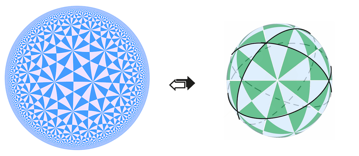
Figure 6: The duality between the hyperbolic plane and sphere is the basic example of the duality between symmetric spaces of compact and noncompact type.

Duality for symmetric spaces generalizes the relationship between spheres and hyperbolic spaces, as well as between classical and hyperbolic trigonometric functions. In the reference Table 6, we provide for each family of symmetric spaces an explicit realization of both the noncompact symmetric space and its compact dual as coset spaces $\mathsf{G}/\mathsf{K}$.

Type	Parameters	Symmetric space
AI	$n=2$	${\rm SL}(2,\mathbb{R})/{\rm SO}(2,\mathbb{R})$	$\mathbb{H}^{2}$
A	$n=2$	${\rm SL}(2,\mathbb{C})/{\rm SU}(2)$	$\mathbb{H}^{3}$
BDI	$p=1$	${\rm SO}(1,q)/{\rm SO}(q)$	$\mathbb{H}^{q}$
AIII	$p=1,q=1$	${\rm SU}(1,1)/{\rm SU}(1)\times{\rm SU}(1)$	$\mathbb{H}^{2}$
CI	$n=1$	${\rm Sp}(2,\mathbb{R})/{\rm U}(1)$	$\mathbb{H}^{2}$
DIII	$n=2$	${\rm SO}^{*}(4)/{\rm U}(1)$	$\mathbb{H}^{2}$
CII	$p=q=1$	${\rm Sp}(1,1)/{\rm Sp}(1)\times{\rm Sp}(1)$	$\mathbb{H}^{4}$
AII	$n=1$	${\rm SL}(2,\mathbb{H})/{\rm Sp}(1)$	$\mathbb{H}^{5}$
D	$n=1$	${\rm SO}(2,\mathbb{C})/{\rm SO}(2)$	$\mathbb{R}^{*}$
B	$n=1$	${\rm SO}(3,\mathbb{C})/{\rm SO}(3)$	$\mathbb{H}^{3}$
C	$n=1$	${\rm Sp}(1,\mathbb{C})/{\rm Sp}(1)$	$\mathbb{H}^{3}$

Table 7: Hyperbolic spaces for low parameters

A.3 Vector-Valued Distance

The familiar geometric invariant of pairs of points is simply the distance between them. For rank $n$ symmetric spaces, this one dimensional invariant is superseded by an $n$-dimensional invariant: the vector valued distance.

Abstractly, one computes this invariant as follows: for a symmetric space $M$ with ${\rm Isom}_{0}(M)=G$, choose a distinguished basepoint $m\in M$, and let $K<G$ be the subgroup of symmetries fixing $m$. Additionally choose a distinguished maximal flat $F\subset M$ containing $m$, and an identification of this flat with $\mathbb{R}^{n}$. Given any pair of points $p,q\in M$, one may find an isometry $g\in G$ moving $p$ to $m$, and $q$ to some other point $g(q)=v\in F$ in the distinguished flat. Under the identification of $F$ with $\mathbb{R}^{n}$, the difference vector $v-m$ is a vector-valued invariant of the original two points, and determines the vector valued distance. (In practice we may arrange so that $m$ is identified with ${\bf 0}$, so this difference is simply $v$).

In rank 1, the flat $F$ identifies with $\mathbb{R}^{1}$, and this difference vector $v-m$ with a number. This number encodes all geometric information about the pair $(p,q)$ invariant under the symmetries of $M$. Indeed, the distance from $p$ to $q$ is simply its absolute value!

In rank $n$, “taking the absolute value” has an $n$-dimensional generalization, via a finite a finite group of symmetries of called the Weyl group. This group $W<K$ acts on the flat $F$, and abstractly, the vector valued distance $\rm{vDist}(p,q)$ from $p$ to $q$ is this difference vector up to the action of the Weyl group. This vector valued distance $\rm{vDist}(p,q)$ is the complete invariant for pairs of points in $M$ - it contains all geometric information about the pair which is invariant under all symmetries. In particular, given the vector valued distance $\rm{vDist}(p,q)$, the (Riemannian) distance from $p$ to $q$ is trivial to compute - it is given by the length of $\rm{vDist}(p,q)$ in $\mathbb{R}^{n}$.

The identification of $F$ with $\mathbb{R}^{n}$ makes this more explicit. Here the Weyl group acts as a group of linear transformations, which divide $\mathbb{R}^{n}$ into a collection of conical fundamental domains for the action, known as Weyl chambers. Choosing a fixed Weyl chamber $C$, we may use these symmetries to move our originally found difference vector $v-m$ into $C$. The vector valued distance is this resulting vector $\rm{vDist}(p,q)\in C$.

Figure 7: A choice of Weyl chamber the Siegel spaces of rank $n$ is given by $C=\{(v_{i})\in\mathbb{R}^{n}\mid v_{1}\geq v_{2}\geq\cdots\geq v_{n}\geq 0\}$. In rank 1, this is the nonnegative reals. Illustrated here are ranks $n=2,3$.

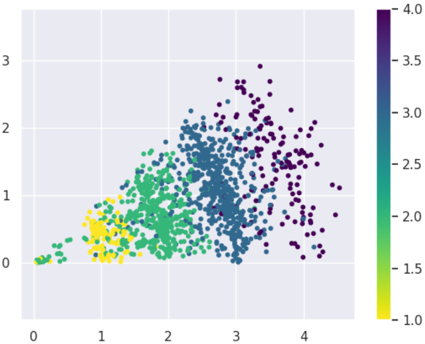
(a)

(b)

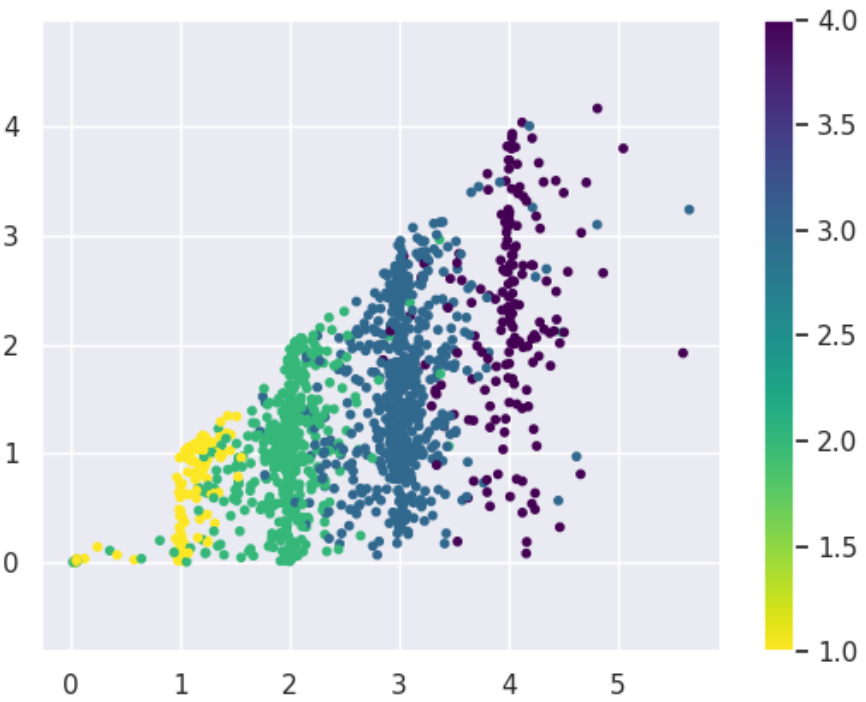
(c)

Figure 14: Plot of $(v_{1},v_{2})$ of $\mathcal{S}_{2}^{R}$ (left), $\mathcal{S}_{2}^{F1}$ (center), and $\mathcal{S}_{2}^{F_{\infty}}$ (right) for vertex pairs sampled from bio-diseasome. Color indicates ground-truth distance.

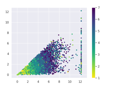
(a)

(b)

(c)

Figure 15: Plot of $(v_{1},v_{2})$ of $\mathcal{S}_{2}^{R}$ (left), $\mathcal{S}_{2}^{F1}$ (center), and $\mathcal{S}_{2}^{F_{\infty}}$ (right) for vertex pairs sampled from csphd. Color indicates ground-truth distance.

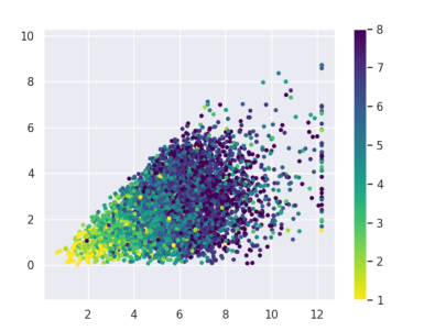
(a)

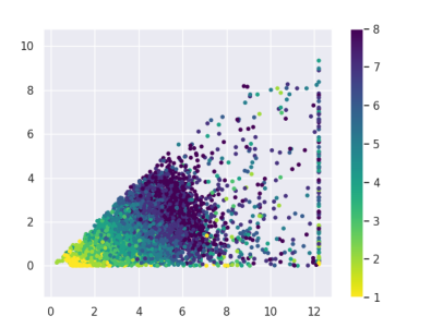
(b)

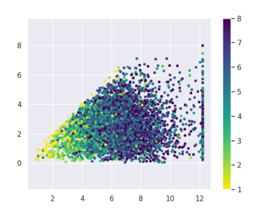
(c)

Figure 16: Plot of $(v_{1},v_{2})$ of $\mathcal{S}_{2}^{R}$ (left), $\mathcal{S}_{2}^{F1}$ (center), and $\mathcal{S}_{2}^{F_{\infty}}$ (right) for vertex pairs sampled from EuroRoad. Color indicates ground-truth distance.

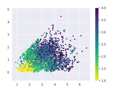
(a)

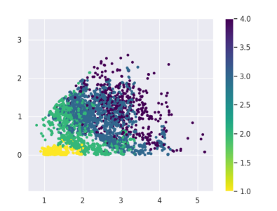
(b)

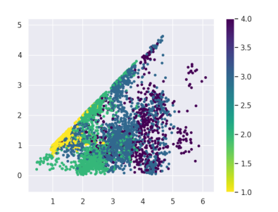
(c)

Figure 17: Plot of $(v_{1},v_{2})$ of $\mathcal{S}_{2}^{R}$ (left), $\mathcal{S}_{2}^{F1}$ (center), and $\mathcal{S}_{2}^{F_{\infty}}$ (right) for vertex pairs sampled from Grid4D. Color indicates ground-truth distance.

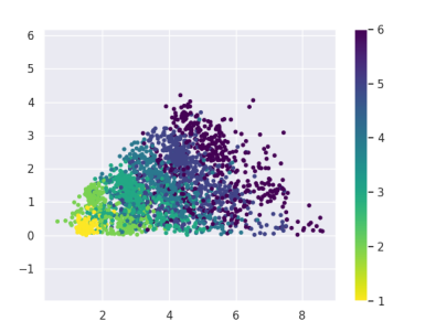
(a)

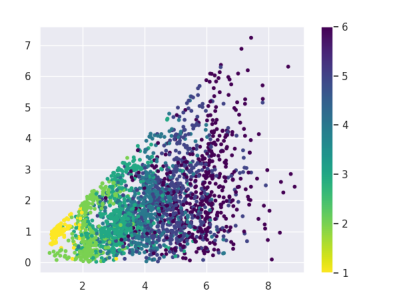
(b)

(c)

Figure 18: Plot of $(v_{1},v_{2})$ of $\mathcal{S}_{2}^{R}$ (left), $\mathcal{S}_{2}^{F1}$ (center), and $\mathcal{S}_{2}^{F_{\infty}}$ (right) for vertex pairs sampled from Tree $\times$ Grid. Color indicates ground-truth distance.

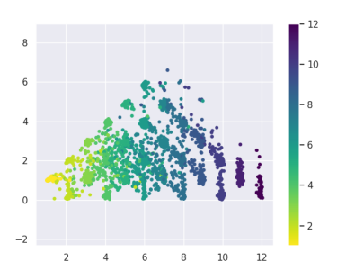
(b)

(c)

Figure 19: Plot of $(v_{1},v_{2})$ of $\mathcal{S}_{2}^{R}$ (left), $\mathcal{S}_{2}^{F1}$ (center), and $\mathcal{S}_{2}^{F_{\infty}}$ (right) for vertex pairs sampled from Tree $\times$ Tree. Color indicates ground-truth distance.

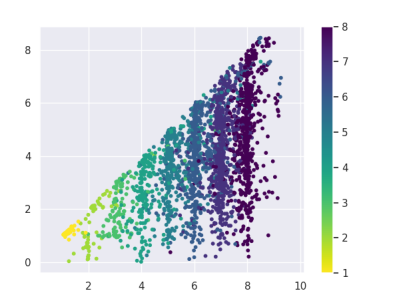
(b)

(c)

Figure 20: Plot of $(v_{1},v_{2})$ of $\mathcal{S}_{2}^{R}$ (left), $\mathcal{S}_{2}^{F1}$ (center), and $\mathcal{S}_{2}^{F_{\infty}}$ (right) for vertex pairs sampled from Tree. Color indicates ground-truth distance.

For example, in rank $n$ Siegel space, the Weyl group acts on $\mathbb{R}^{2}$ by the reflection symmetries of a cube, and a choice of Weyl chamber amounts to a choice of linear ordering of the vector components with respect to zero. One choice is shown in Figure 7. In rank 2, this chamber is used to display the vector valued distances associated to edges and nodes of an embedded graph in Figures 13-20. Note that once a Weyl chamber is picked it may be possible to find the vector valued distance corresponding to a vector in $\mathbb{R}^{n}$ without explicit use of the Weyl group: for the Siegel spaces this is by sorting the vector components in nondecreasing order.

Computing Distance: The process for computing the vector valued distance is summarized below. It is explicitly carried out for the Siegel spaces and their compact duals in Appendix B.

Let $M,G,K,F,m$ be as in the previous section. Choose an identification $\phi\colon F\to\mathbb{R}^{n}$ which sends the basepoint $m$ to $\bf{0}$, and a Weyl chamber $C\subset\mathbb{R}^{n}$ for the Weyl group $W$. For any pair of points $p,q\in M$;

1. Move $p$ to the basepoint:
   Compute $g\in G$ such that $g(p)=m$.

2. Move $q$ into the flat:
   Compute $k\in K$ such that $k(g(q))\in F$. Now both $g(p)=m$ and $k(g(q))$ lie in the distinguished flat $F$.

3. Identify the flat with $\mathbb{R}^{n}$:
   Compute $u=\phi(k(g(q)))\in\mathbb{R}^{n}$. The points ${\bf 0}$ and $u$ represent $p,q$ after being moved into the flat, respectively.

4. Return the Vector Valued Distance:
   Compute $v\in C$ such that $v=Au$ for some element $A\in W$. This is the vector valued distance $\rm{vDist}(p,q)$

The Riemannian distance is computed directly from the vector valued distance as its Euclidean norm, ${\rm dist}(p,q)=\|{\rm vDist}(p,q)\|$.

A.4 Finsler Metrics

A Riemannian metric on a manifold $M$ is defined by a smooth choice of inner product on the tangent bundle. Finsler metrics generalize this by requiring only a smoothly varying choice of norm $\|\cdot\|_{F}$. The length of a curve $\gamma$ is defined via integration of this norm along the path

$$\mathrm{Length}_{F}(\gamma)=\int_{I}\|\gamma^{\prime}\|_{F}dt,$$

and the distance between points by the infimum of this over all rectifiable curves joining them

$$d_{F}(p,q)=\inf\{\mathrm{Length}_{F}(\gamma)\mid\gamma(0)=p,\;\gamma(1)=q\}$$

The geometry of symmetric spaces allows the computation of Finsler distances, like much else, to take place in a chosen maximal flat. On such flat spaces, the ability to identify all tangent spaces allow particularly simple Finsler metrics to be defined by choosing a single norm on $\mathbb{R}^{n}$. We quickly review this theory below.

Finsler Metrics on $\mathbb{R}^{n}$: Any norm on $\mathbb{R}^{n}$ defines a Finsler metric. As norms on a vector space are uniquely determined by their unit spheres, the data of a Finsler metric is given by a convex polytope $S$ containing $\bf{0}$. An important example in this work is the $\ell^{1}$ Finsler metric on $\mathbb{R}^{n}$, given by the norm $\|(x_{i})\|_{\ell^{1}}=\sum_{i}|x_{i}|$. Its unit sphere is the boundary of the dual to the $n$-dimensional cube (in $\mathbb{R}^{2}$, this is again a square, but oriented at $45^{\circ}$ with respect to the coordinate axes).

Given such an $P$, the Finsler norm $\|v\|_{F}$ of a vector $v\in\mathbb{R}^{n}$ is the unique positive $\ell$ such that $\frac{1}{\ell}v\in\partial P$. Figure 8 below shows the spheres of radius $1$ and $2$ with respect to the $\ell^{1}$ metric on the plane.

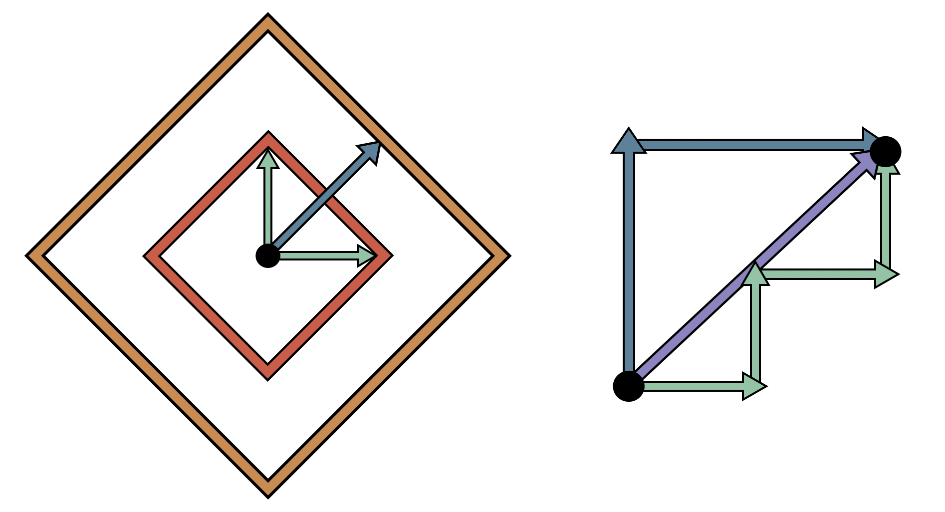
Figure 8: Left: Vectors of length 1 and 2 with respect to the $\ell^{1}$ norm on $\mathbb{R}^{2}$. Right: three geodesics of length 4 in the $\ell^{1}$ metric (to same scale as left image).

While affine lines are geodesics in Finsler geometry, they need not be the unique geodesics between a pair of points. Consider again Figure 8: the vector sum of the two unit vectors in is exactly the diagonal vector, which lies on the $\ell^{1}$ sphere of radius $2$. That is, in $\ell^{1}$ geometry traveling along the diagonal, or along the union of a vertical and horizontal side of a square both are distance minimizing paths of length 2. The $\ell^{1}$ metric is often called the ‘taxicab’ metric for this reason: much as in a city with a grid layout of streets, there are many shortest paths between a generic pair of points, as you may break your path into different choices of horizontal and vertical segments without changing its length. See Figure 2 in the main text for another example of this.

Finsler Metrics on Symmetric Spaces: To define a Finsler metric on a symmetric space $M$, it suffices to define it on a chosen maximal flat, and evaluate on arbitrary pairs of points with the help of the vector valued distance. To induce a well defined Finsler metric $M$, a norm on this designated flat need only be invariant under the Weyl group $W$. Said geometrically, the unit sphere of the norm $\|\cdot\|_{F}$ needs to contain it as a subgroup of its symmetries. Given such a norm, the Finsler distance between two points is simply the Finsler norm of their vector valued distance

$$d_{F}(p,q)=\|{\rm vDist}(p,q)\|_{F}.$$

Consequentially once the vector valued distance is known, any selection of Riemannian or Finsler distances may be computed at marginal additional cost.

Figure 9: The unit spheres of several Finsler metrics on $\mathbb{R}^{3}$ invariant under the Weyl group of the rank 3 Siegel space. The octahedron induces the $\ell^{1}$ metric.

A.5 Local Geometry for Riemannian Optimization

Different Riemannian optimization methods require various input from the local geometry - here we describe a computation of the Riemannian gradient, parallel transport and the exponential map for general irreducible symmetric spaces.

Riemannian Gradient Given a function $f\colon M\to\mathbb{R}$, the differential of $f$ is a 1-form which measures how infinitesimal changes in the input affects (infinitesimally) the output. More precisely at each point $p\in M$, $df$ is a linear functional on $T_{p}M$ sending a vector $v$ to the directional derivative $df_{p}(v)$ of $f$ in direction $v$.

In Euclidean space, this data is conveniently expressed as a vector: the gradient $\nabla f$ defined such that $(\nabla f(p))\cdot v=df_{p}(v)$. This extends directly to any Riemannian manifold, where the dot product is replaced with the Riemannian metric. That is, the Riemannian gradient of a function $f\colon M\to\mathbb{R}$ is the vector field $grad_{R}(f)$ on $M$ such that

$$g_{p}(\mathrm{grad}_{R}(f),v)=df_{p}(v)$$

for every $p\in M$, $v\in T_{p}M$. Given a particular model (and thus, a particular coordinate system and metric tensor) one may use this implicit definition to give a formula for $\mathrm{grad}_{R}$. See Appendix B.6 for an explicit example, deriving the Riemannian gradient for Siegel space from its metric tensor.

Parallel Transport

While the lack of curvature in Euclidean space allows all tangent spaces to be identified, in general symmetric spaces the result of transporting a vector from one tangent space to another is a nontrivial, path dependent operation. This parallel transport assigns to a path $\gamma$ in $M$ from $p$ to $q$ an isomorphism $P_{\gamma}\colon T_{p}M\to T_{q}M$ interpreted as taking a vector $v\in T_{p}M$ at $p$ to $P_{\gamma}(v)\in T_{q}M$ by “moving without turning” along $\gamma$.

The computation of parallel transport along geodesics in a symmetric space is possible directly from the isometry group. To fix notation, for each $m\in M$ let $\sigma_{m}\in G$ be the geodesic reflection fixing $m$. Let $\gamma$ be a geodesic in $M$ through $p$ at $t=0$. As $t$ varies, the isometries $\tau_{t}=\sigma_{\gamma(t/2)}\circ\sigma_{p}$, called transvections, form the 1-parameter subgroup of translations along $\gamma$. If $p,q\in M$ are two points at distance $L$ apart along the the geodesic $\gamma$, the transvection $\tau_{L}$ takes $p$ to $q$, and its derivative $(d\tau_{L})_{p}=P_{\gamma}\colon T_{p}M\to T_{q}M$ performs the parallel transport for $\gamma$.

The Exponential Map & Lie Algebra The exponential map for a Riemannian manifold $M$ is the map $\exp\colon TM\to M$ such that if $v\in T_{p}(X)$, $\exp(v)$ is the point in $M$ reached by traveling distance $\|v\|$ along the geodesic on $M$ through $p$ with initial direction parallel to $v$.

When $M$ is a symmetric space with symmetry group $G$, this may be computed using the Lie group exponential $\exp\colon\mathfrak{g}\to G$ (the matrix exponential, when $G$ is a matrix Lie group). Choose a point $p\in M$ and let $\sigma_{p}$ be the geodesic reflection in $p$. Then $\sigma_{p}$ defines an involution $G\to G$ by $g\mapsto\sigma_{p}\circ g\circ\sigma_{p}$ (where composition is as isometries of $M$), and the eigenspaces of the differential of this involtuion give a decomposition $\mathfrak{g}=\mathfrak{k}\oplus\mathfrak{p}$ into the $+1$ eigenspace $\mathfrak{k}$ and the $-1$ eigenspace $\mathfrak{p}$. Here $\mathfrak{k}$ is the Lie algebra of the stabilizer $K=\mathfrak{stab}(p)<G$, and so $\mathfrak{p}$ identifies with $T_{p}M$ under the differential of the quotient $G\to G/K\cong M$.

Let $\phi\colon T_{p}M\to\mathfrak{p}$ be the inverse of this identification. Then for a vector $v\in T_{p}M$, we may find the point $q=\exp_{p}(v)\in M$ as follows:

1. Compute $\phi(v)=A\in\mathfrak{p}$. This is the tangent vector $v$, viewed as a matrix in the Lie algebra to $G$.

2. Compute $g=\exp(A)$, where $\exp$ is the matrix exponential.

3. Use the action of $G$ on $M$ by isometries to compute $q=g(p)$.

Appendix B Explicit Formulas for Siegel Spaces

This section gives the calculations mathematics required to implement two models of Siegel space (the bounded domain model and upper half space) as well as a model of its compact dual.

B.1 Linear Algebra Conventions

A few clarifications from linear algebra can be useful:

1. The inverse of a matrix $X^{-1}$, the product of two matrices $XY$, the square $X^{2}$ of a square matrix are understood with respect to the matrix operations. Unless all matrices are diagonal these are different than doing the same operation to each entry of the matrix.

2. If $Z=X+iY$ is a complex matrix,

   • $Z^{t}$ denotes the transpose matrix, i.e. $(Z^{t})_{ij}=Z_{ji}$,

   • $\overline{Z}=X-iY$ denotes the complex conjugate

   • $X^{*}$ denotes its transpose conjugate, i.e. $X^{*}=\overline{X^{t}}$.

3. A complex square matrix $Z$ is Hermitian if $Z^{*}=Z$. In this case its eigenvalues are real and positive. It is unitary if $Z^{*}=Z^{-1}$. In this case its eigenvalues are complex numbers of absolute value 1 (i.e. points in the unit circle).

4. If $X$ is a real symmetric, or complex Hermitian matrix, $X>\!\!>0$ means that $X$ is positive definite, equivalently all its eigenvalues are bigger than zero.

B.2 Takagi Factorization

Given a complex symmetric matrix $A$, the Takagi factorization is an algorithm that computes a real diagonal matrix $D$ and a complex unitary matrix $K$ such that

$$A=\overline{K}DK^{*}.$$

This will be useful to work with the bounded domain model. It is done in a few steps

1. Find $Z_{1}$ unitary, $D$ real diagonal such that

   $$A^{*}A=Z_{1}^{*}D^{2}Z_{1}$$

2. Find $Z_{2}$ orthogonal, $B$ complex diagonal such that

   $$\overline{Z}_{1}AZ_{1}^{*}=Z_{2}BZ_{2}^{t}$$

   This is possible since the real and imaginary parts of $\overline{Z}_{1}AZ_{1}^{*}$ are symmetric and commute, and are therefore diagonalizable in the same orthogonal basis.

3. Set $Z_{3}$ be the diagonal matrix with entries

   $$(Z_{3})_{ii}=\left(\sqrt{\frac{b_{i}}{|b_{i}|}}\right)^{-1}$$

   where $b_{i}=(B)_{ii}$

4. Set $K=Z_{1}^{*}Z_{2}Z_{3}$, $D$ as in Step 1. It then holds

   $$A=\overline{K}DK^{*}.$$

B.3 Siegel Space and its Models

We consider two models for the symmetric space, the bounded domain

$$\mathcal{B}_{n}:=\{Z\in{\rm Sym}(n,\mathbb{C})|\;{\rm Id}-Z^{*}Z>\!\!>0\}$$

and the upper half space

$$\mathcal{S}_{n}:=\{X+iY\in{\rm Sym}(n,\mathbb{C})|\;Y>\!\!>0\}.$$

An explicit isomorphism between the two domains is given by the Cayley transform

$$\begin{array}[]{cccc}c:&\mathcal{B}_{n}&\to&\mathcal{S}_{n}\\ &Z&\mapsto&i(Z+{\rm Id})(Z-{\rm Id})^{-1}\end{array}$$

whose inverse $c^{-1}=t$ is given by

$$\begin{array}[]{cccc}t:&\mathcal{S}_{n}&\to&\mathcal{B}_{n}\\ &X&\mapsto&(X-i{\rm Id})(X+i{\rm Id})^{-1}\end{array}$$

When needed, a choice of basepoint for these models is $i{\rm Id}\in\mathcal{S}_{n}$ for upper half space and the zero matrix ${\bf 0}\in\mathcal{B}_{n}$ for the bounded domain. A convenient choice of maximal flats containing these basepoints are the subspaces $\{iD\mid D={\rm diag}(d_{i}),\;d_{i}>0\}\subset\mathcal{S}_{n}$ and $\{D={\rm diag}(d_{i})\mid d_{i}\in(-1,1)\}\subset\mathcal{B}_{n}$.

The group of symmetries of the Siegel space $\mathcal{S}_{n}$ is ${\rm Sp}(2n,\mathbb{R})$, the subgroup of ${\rm SL}(2n,\mathbb{R})$ preserving a symplectic form: a non-degenerate antisymmetric bilinear form on $\mathbb{R}^{2n}$. In this text we will choose the symplectic form represented, with respect to the standard basis, by the matrix $\left(\begin{smallmatrix}0&{\rm Id}_{n}\\ -{\rm Id}_{n}&0\end{smallmatrix}\right)$ so that the symplectic group is given by the matrices that have the block expression

$$\left\{\begin{pmatrix}A&B\\ C&D\end{pmatrix}\left|\begin{array}[]{l}A^{t}D-C^{t}B={\rm Id}\\ A^{t}C=C^{t}A\\ B^{t}D=D^{t}B\end{array}\right.\right\}$$

where $A,B,C,D$ are real $n\times n$ matrices.

The symplectic group ${\rm Sp}(2n,\mathbb{R})$ acts on $\mathcal{S}_{n}$ by non-commutative fractional linear transformations

$$\begin{pmatrix}A&B\\ C&D\end{pmatrix}\cdot Z=(AZ+B)(CZ+D)^{-1}.$$

The action of ${\rm Sp}(2n,\mathbb{R})$ on $\mathcal{B}_{n}$ can be obtained through the Cayley transform.

B.4 Computing the Vector-Valued Distance

The Riemannian metric, as well as any desired Finsler distance, are computable directly from the vector-valued distance as explained in Appendix A.3. Following those steps, we give an explicit implementation for the upper half space model below, and subsequently use the Cayley transform to extend this to the bounded domain model.

Given as input two points $Z_{1},Z_{2}\in\mathcal{S}_{n}$ we perform the following computations:

1) Move $Z_{1}$ to the basepoint: Compute the image of $Z_{2}$ under the transformation taking $Z_{1}$ to $iI$, defining

$$Z_{3}:=\sqrt{\Im Z_{1}}^{-1}(Z_{2}-\Re Z_{1})\sqrt{\Im Z_{1}}^{-1}\in\mathcal{S}_{n}$$

2) Move $Z_{2}$ into the chosen flat: Define

$$W=t(Z_{3})\in\mathcal{B},$$

and use the Takagi factorization to write

$$W=\overline{K}DK^{*}$$

for some real diagonal matrix $D$ with eigenvalues between 0 and 1, and some unitary matrix $K$. Note: to make computations easier, we are leveraging the geometry of both models here, so in fact $i(I+D)(I-D)^{-1}$ is the matrix lying in the standard flat containing $iI$.

3) Identify the flat with $\mathbb{R}^{n}$: Define the vector $v=(v_{i})\in\mathbb{R}^{n}$ with

$$v_{i}=\log\frac{1+d_{i}}{1-d_{i}},$$

for $d_{i}$ the $i^{th}$ diagonal entry of the matrix $D$ from the last step.

4) Return the Vector Valued Distance: Sort the absolute values of the entries of $v$ to be in nonincreasing order, and set $\mathrm{vDist}(Z_{1},Z_{2})$ equal to the resulting list.

$$\mathrm{vDist}=(|v_{i_{1}}|,|v_{i_{2}}|,\ldots,|v_{i_{n}}|)$$

$$|v_{i_{1}}|\geq|v_{i_{2}}|\geq\cdots\geq|v_{i_{n}}|$$

Bounded domain: In this case, given $W_{1},W_{2}\in\mathcal{B}$ we consider the pair $Z_{1},Z_{2}\in\mathcal{S}_{n}$ obtained applying the Cayley transform $Z_{i}=t(W_{i})$. Then we can apply the previous algorithm, indeed

$$\mathrm{vDist}(W_{1},W_{2})=\mathrm{vDist}(Z_{1},Z_{2}).$$

B.5 Riemannian & Finsler Distances

The Riemannian distance between two points $X,Y$ in the Siegel space (either the upper half space or bounded domain model) is induced by the Euclidean metric on its maximal flats. This is calculable directly from the vector valued distance $\mathrm{vDist}(X,Y)=(v_{1},v_{2},\ldots,v_{n})$ as

$$d^{R}(X,Y)=\sqrt{\sum_{i=1}^{n}v_{i}^{2}}.$$

The Weyl group for the rank $n$ Siegel space is the symmetry group of the $n$ cube. Thus, any Finsler metric on $\mathbb{R}^{n}$ whose unit sphere has these symmetries has these symmetries induces a Finsler metric on Siegel space. The class of such finsler metrics includes many well-known examples such as the $\ell^{p}$ metrics

$$\|(v_{1},\ldots,v_{n})\|_{\ell^{p}}=\left(\sum_{i}|v_{i}|^{p}\right)^{\frac{1}{p}},$$

which is one of the reasons the Siegel space is an attractive avenue for experimentation.

Of particular interest are the $\ell^{1}$ and $\ell^{\infty}$ Finsler metrics. The distance functions induced on the Siegel space by them are given below

$$d^{F_{1}}(X,Y)=\sum_{i=1}^{n}v_{i}\qquad d^{F_{\infty}}(X,Y)=v_{1}.$$

Where $X,Y$ are points in Siegel space (again, either in the upper half space or bounded domain models), and the $v_{i}$ are the component of the vector valued distance $\mathrm{vDist}(X,Y)=(v_{1},v_{2},\ldots,v_{n})$.

There are explicit bounds between the distances, for example

$$\frac{1}{\sqrt{n}}d^{F_{1}}(X,Y)\leq d^{R}(X,Y)\leq d^{F_{1}}(X,Y)$$ (4)

Furthermore, we have

$$\begin{split}d^{F_{1}}(X,Y)=\log\det(\sqrt{R(X,Y)}+{\rm Id})-\\ \log\det({\rm Id}-\sqrt{R(X,Y)})\end{split}$$ (5)

which, in turn, allows to estimate the Riemannian distance using (4).

B.6 Riemannian Gradient

We consider on ${\rm Sym}(n,\mathbb{C})$ the Euclidean metric given by

$$\|V\|_{E}^{2}={\rm tr}(V\overline{V}),$$

here ${\rm tr}$ denotes the trace, and, as above, $V\overline{V}$ denotes the matrix product of the matrix $V$ and its conjugate.

Siegel upperhalf space: The Riemannian metric at a point $Z\in\mathcal{S}_{n}$, where $Z=X+iY$ is given by (Siegel, 1943)

$$\|V\|_{R}^{2}={\rm tr}(Y^{-1}VY^{-1}\overline{V}).$$

As a result we deduce that

$${\rm grad}(f(Z))=Y\cdot{\rm grad_{E}}(f(Z))\cdot Y$$

Bounded domain: In this case we have

$${\rm grad}(f(Z))=A\cdot{\rm grad_{E}}(f(Z))\cdot A$$

where $A={\rm Id}-\overline{Z}Z$

B.7 Embedding Initialization

Different embeddings methods initialize the points close to a fixed basepoint. In this manner, no a priori bias is introduced in the model, since all the embeddings start with similar values.

We use the basepoints specified previously: $i{\rm Id}$ for Siegel upper half space and ${\bf 0}$ for the bounded domain model.

In order to produce a random point we generate a random symmetric matrix with small entries and add it to our basepoint. As soon as all entries of the perturbation are smaller than $1/n$ the resulting matrix necessarily belongs to the model. In our experiments, we generate random symmetric matrices with entries taken from a uniform distribution $\mathcal{U}(-0.001,0.001)$.

B.8 Projecting Back to the Models

The goal of this section is to explain two algorithms that, given $\epsilon$ and a point $Z\in{\rm Sym}(n,\mathbb{C})$, return a point $Z_{\epsilon}^{\mathcal{S}}$ (resp. $Z_{\epsilon}^{\mathcal{B}}$), a point close to the original point lying in the $\epsilon$-interior of the model. This is the equivalent of the projection applied in Nickel & Kiela (2017) to constrain the embeddings to remain within the Poincaré ball, but adapted to the structure of the model. Observe that the projections are not conjugated through the Cayley transform.

Siegel upperhalf space: In the case of the Siegel upperhalf space $\mathcal{S}_{n}$ given a point $Z=X+iY\in{\rm Sym}(n,\mathbb{C})$

1. Find a real $n$-dimensional diagonal matrix $D$ and an orthogonal matrix $K$ such that

   $$Y=K^{t}DK$$

2. Compute the diagonal matrix $D_{\epsilon}$ with the property that

   $$(D_{\epsilon})_{ii}=\begin{cases}D_{ii}&\text{ if }D_{ii}>\epsilon\\ \epsilon&\text{ otherwise}\end{cases}$$

3. The projection is given by

   $$Z_{\epsilon}^{\mathcal{S}}:=X+iK^{t}D_{\epsilon}K$$

Bounded Domain: In the case of the bounded domain $\mathcal{B}$ given a point $Z=X+iY\in{\rm Sym}(n,\mathbb{C})$

1. Use the Takagi factorization to find a real $n$-dimensional diagonal matrix $D$ and an unitary matrix $K$ such that

   $$Y=\overline{K}DK^{*}$$

2. Compute the diagonal matrix $D^{\mathcal{B}}_{\epsilon}$ with the property that

   $$(D_{\epsilon}^{\mathcal{B}})_{ii}=\begin{cases}D_{ii}&\text{ if }D_{ii}<1-\epsilon\\ 1-\epsilon&\text{ otherwise }\end{cases}$$

3. The projection is given by

   $$Z_{\epsilon}^{\mathcal{B}}:=\overline{K}D^{\mathcal{B}}_{\epsilon}K^{*}$$

B.9 Crossratio and Distance

Given two points $X,Y$ in Siegel space, there is an alternative means of calculating the vector valued distance (and thus any Riemannian or Finsler distance one wishes) via an invariant known as the cross ratio.

Siegel upperhalf space: Given two points $X,Y\in\mathcal{S}_{n}$ their crossratio is given by the complex $n\times n$-matrix

$$R_{\mathcal{S}}(X,Y)=(X-Y)(X-\overline{Y})^{-1}(\overline{X}-\overline{Y})(\overline{X}-Y)^{-1}.$$

It was established by Siegel (Siegel, 1943) that if $r_{1},\ldots,r_{n}$ denote the eigenvalues of $R$ (which are necessarily real greater than or equal to 1) and we denote by $v_{i}$ the numbers

$$v_{i}=\log{\frac{1+\sqrt{r}_{i}}{1-\sqrt{r}_{i}}}$$

then the $v_{i}$ are the components of the vector-valued distandce $\mathrm{vDist}(X,Y)$. Thus, the Riemannian distance is

$$d^{R}(X,Y)=\sqrt{\sum_{i=1}^{n}v_{i}^{2}}.$$

The Finsler distances $d^{F_{1}}$ and $d^{F_{\infty}}$ are likewise given by the same formulas as previously.

In general it is computationally difficult to compute the eigenvalues, or the squareroot, of a general complex matrix. However, we can use the determinant $\det_{R}$ of the matrix $R(X,Y)$ to give a lower bound on the distance:

$$\log{\frac{1+\sqrt{\det_{R}}}{1-\sqrt{\det_{R}}}}\leq d^{R}(X,Y).$$

Bounded domain: The same study applies to pairs of points $X,Y\in\mathcal{B}$, but their crossratio should be replaced by the expression

$$\begin{split}R_{\mathcal{B}}(X,Y)=(X-Y)(X-\overline{Y^{-1}})^{-1}\\ (\overline{X^{-1}}-\overline{Y^{-1}})(\overline{X^{-1}}-Y)^{-1}\end{split}$$ (6)

B.10 The Compact Dual of the Siegel Space

The compact dual to the (non-positively) curved Siegel space is a compact non-negatively curved symmetric space; in rank $1$ this is just the 2-sphere. Many computations in the compact dual are analogous to those for the Siegel spaces, and are presented below.

Model

Abstractly, the compact dual is the space of complex structures on quaternionic $n$-dimensional space compatible with a fixed inner product. It is convenient to work with a coordinate chart, or affine path covering all but a measure zero subset of this space. We denote this patch by $\mathcal{D}_{n}$, which consists of all $n\times n$ complex symmetric matrices:

$$\mathcal{D}_{n}={\rm Sym}(n;\mathbb{C})$$

With this choice of model, tangent vectors to $\mathcal{D}_{n}$ are also represented by complex symmetric matrices. More precisely, for each $W\in\mathcal{D}_{n}$ we may identify the tangent space $T_{W}\mathcal{D}_{n}$ with ${\rm Sym}(n,\mathbb{C})$.

Basepoint: The basepoint of $\mathcal{D}_{n}$ is the zero matrix $\bf{0}$.

Maximal Flat: A useful choice of maximal flat is the subspace of real diagonal matrices.

Projection: The model $\mathcal{D}_{n}$ is a linear subspace of the space of $n\times n$ complex matrices. Orthogonal projection onto this subspace is given by symmetrization,

$$W\mapsto\frac{1}{2}(W+W^{t}).$$

Isometries: The symmetries of the compact dual are given by the compact symplectic group ${\rm Sp}(n)$. With respect to the model $\mathcal{D}_{n}$, we may realize this as the intersection of the complex symplectic group ${\rm Sp}(2n,\mathbb{C})$ and the unitary group $U(2n,\mathbb{C})$

$$\left\{\begin{pmatrix}A&B\\ C&D\end{pmatrix}\left|\begin{array}[]{l}A^{t}D-C^{t}B={\rm Id}\\ A^{t}C=C^{t}A\\ B^{t}D=D^{t}B\\ A^{\ast}A+C^{\ast}C={\rm Id}\\ B^{\ast}B+D^{\ast}D={\rm Id}\\ A^{\ast}B+C^{\ast}D=0\end{array}\right.\right\}$$

where $A,B,C,D$ are complex $n\times n$ matrices. The first four conditions are analogs of those defining ${\rm Sp}(2n;\mathbb{R})$, and the final three come from the defining property that a unitary matrix $M$ satisfies $M^{\ast}M={\rm Id}$.

This group acts on $\mathcal{D}_{n}$ by non-commutative fractional linear transformations

$$\begin{pmatrix}A&B\\ C&D\end{pmatrix}\cdot W=(AW+B)(CW+D)^{-1}.$$

Riemannian Metric & Gradient: The Riemannian metric at a point $W\in\mathcal{D}_{n}$ is given by

$$\langle U,V\rangle_{W}=({\rm Id}+\overline{W}W)^{-1}U({\rm Id}+\overline{W}W)^{-1}\overline{V},$$

where $U,V$ are tangent vectors at $W$.

The gradient of a function on the compact dual can be written in terms of its Euclidean gradient, via a formula very similar to that for the Bounded Domain model of the Siegel space. In this case we have

$${\rm grad}(f(W))=A\cdot{\rm grad_{E}}(f(W))\cdot A$$

where (the only difference from the bounded domain version being that the $-$ sign in the definition of $A$ has been replaced with a $+$).

Vector Valued Distance

We again give an explicit implementation of the abstract procedure described in Appendix A.3, to calculate the vector valued distance associated to an arbitrary pair $W_{1},W_{2}\in\mathcal{D}_{n}$ as follows:

Move $W1$ to the basepoint:

1. Use the Takagi factorization to write

   $$W_{1}=\overline{U}PU^{\ast}$$

   for a unitary matrix $U$ and real diagonal matrix $P$.

2. From $P$, we build the diagonal matrix $A=({\rm Id}+P^{2})^{-1/2}$. That is, the diagonal entries of $A$ are $a_{i}=\frac{1}{\sqrt{1+p_{i}^{2}}}$ for $p_{i}$ the diagonal entries of $P$.

3. From $A,U$ we build the following elements $M,R\in{\rm Sp}(n)$ of the compact symplectic group:

   $$M=\begin{pmatrix}A&-AP\\ AP&A\end{pmatrix}\hskip 14.22636ptR=\begin{pmatrix}U^{t}&0\\ 0&U^{\ast}\end{pmatrix}$$

We now use the transformation $M\cdot R$ to move the pair $(W_{1},W_{2})$ to a pair $({\bf 0},Z)$. Because $W_{1}$ ends at the basepoint by construction, we focus on $W_{2}$.

1. Compute $X=R.W_{2}$, that is $X=U^{t}W_{2}U$.

2. Compute $Z=M.X$, that is $Z=(AX-AP)(APX-A)^{-1}$. Alternatively, this simplifies to the conjugation $Z=AYA^{-1}$ by $A$ of the matrix $Y=(X-P)(PX-{\rm Id})^{-1}$

Move $Z$ into the chosen flat: Use the Takagi factorization to write

$$Z=\overline{K}DK^{\ast}$$

for a unitary matrix $K$ and real diagonal matrix $D$.

Identify the Flat with $\mathbb{R}^{n}$: Produce from $D$ the $n$-vector

$$v=(\arctan(d_{1}),\ldots\arctan(d_{n}))$$

Where $(d_{1},\ldots d_{n})$ are the diagonal entries of $D$.

Return the Vector Valued Distance: Order the the entries of $v$ in nondecreasing order. This is the vector valued distance.

$$\mathrm{vDist}=(v_{i_{1}},v_{i_{2}},\ldots,v_{i_{n}})$$

$$v_{i_{1}}\geq v_{i_{2}}\geq\cdots\geq v_{i_{n}}\geq 0$$

Riemannian and Finsler Distances:

The Riemannian distance between two points $X,Y$ in the compact dual is calculable directly from the vector valued distance $\mathrm{vDist}(X,Y)=(v_{1},v_{2},\ldots,v_{n})$ as

$$d^{R}(X,Y)=\sqrt{\sum_{i=1}^{n}v_{i}^{2}}.$$

The Weyl group for the compact dual is the same as for Seigel space, the symmetries of the $n$-cube. Thus the same collection of Finsler metrics induce distance functions on the compact dual, and their formulas in terms of the vector valued distance are unchanged.

$$d^{F_{1}}(X,Y)=\sum_{i=1}^{n}v_{i}\qquad d^{F_{\infty}}(X,Y)=v_{1}.$$

B.11 Interpolation between Siegel Space and its Compact Dual

The Siegel space and its compact dual are part of a 1-parameter family of spaces indexed by a real parameter $k\in\mathbb{R}$. When $n=1$ the symmetric spaces are two-dimensional, and this $k$ is interpreted as their (constant) curvature. That is, this family represents an interpolation between the hyperbolic plane ($k=-1$) and the sphere ($k=1$) through Euclidean space $(k=0)$ as schematically represented in Figure 10. Below we describe the generalization of this to all $n$, by giving the model, symmetries, and distance functions in terms of the parameter $k\in\mathbb{R}$.

Figure 10: A 1-parameter family of spaces interpolating between the Siegel space and its compact dual, here illustrated in rank 1 ($\mathbb{H}^{2}$ transitioning $S^{2}$ through the Euclidean plane with $k=0$).

Model: Our models are most similar to the Bounded domain model of Siegel space, and so we use notation to match. For each $k\in\mathbb{R}$ we define the subset $\mathcal{B}_{n}^{k}$ of ${\rm Sym}(n,\mathbb{C})$ as follows:

$$\mathcal{B}_{n}^{k}=\left\{\begin{matrix}\{W\mid{\rm Id}+kW^{\ast}W>>0\}&k<0\\ {\rm Sym}(n,\mathbb{C})&k\geq 0\end{matrix}\right.$$

The basepoint for $\mathcal{B}_{n}^{k}$ is the zero matrix ${\bf 0}$ for all $k$. Projection back to the model is analogous to what is done for the bounded domain when $k<0$, and is just symmetrization for $k\geq 0$.

Isometries: Denote by $G^{k}$ the isometry group of $\mathcal{B}_{n}^{k}$. A uniform description of $G^{k}$ can be given in close analogy to the description of the symmetries of the compact dual. For each $k\in\mathbb{R}$, $G^{k}={\rm Sp}(2n,\mathbb{C})\cap\mathcal{U}^{k}$ where $\mathcal{U}^{k}$ is a generalization of the usual unitary group

$$\mathcal{U}^{k}=\left\{M\mid M^{\ast}\left(\begin{smallmatrix}k{\rm Id}&0\\ 0&{\rm Id}\end{smallmatrix}\right)M=\left(\begin{smallmatrix}k{\rm Id}&0\\ 0&{\rm Id}\end{smallmatrix}\right)\right\}$$

Riemannian Geometry: The Riemannian metric at a point $W\in\mathcal{B}_{n}^{k}$ is given by the formula

$$\langle U,V\rangle_{W}^{k}={\rm tr}\left(A^{-1}UA^{-1}\overline{V}\right)$$

Where $A={\rm Id}+k\overline{W}W$. As before, this allows us to compute the Riemannian Gradient in terms of the Euclidean gradient on $\mathcal{B}^{k}_{n}$:

$${\rm grad}(f(W))=A\cdot{\rm grad_{E}}(f(W))\cdot A$$

From the Riemannian metric we may explicitly compute the distance function from the basepoint ${\bf 0}$ to a real diagonal matrix $D\in\mathcal{B}_{n}^{k}$:

$$\mathrm{dist}^{k}({\bf 0},D)=\left\{\begin{matrix}\sqrt{\sum_{i}\frac{\mathrm{arctanh}\left(d_{i}\sqrt{|k|}\right)^{2}}{\sqrt{|k|}}}&k<0\\ \sqrt{\sum_{i}d_{i}^{2}}&k=0\\ \sqrt{\sum_{i}\frac{\arctan\left(d_{i}\sqrt{k}\right)^{2}}{\sqrt{k}}}&k>0\end{matrix}\right.$$

Distance: The seven step procedure for calculating distance in the compact dual can be modified to give a procedure for the distance in $\mathcal{B}_{n}^{k}$. To calculate the Riemannian distance, Step 7 must be replaced with the distance formula above. The only other changes involve the construction of the matrix called $M$

• In step 2, the computation of $P$ is unchanged but $A$ is replaced with $A=({\rm Id}+kP^{2})^{-1/2}$.

• In step 3, the matrix $M$ is replaced with

  $$M=\begin{pmatrix}A&-AP\\ \mathrm{sgn}(k)AP&A\end{pmatrix}$$

Where $\mathrm{sgn}(k)=0$ if $k=0$. Note the computation of $M.X$ in Step 5 also changes, as $M$ has changed. Now $M.X=(AX-AP)(\mathrm{sgn}(k)APX-A)^{-1}$.

B.12 Experiments on the Compact Dual

We perform experiments on small synthetic datasets to compare the performance of the dual model to the upper half Siegel space and the Bounded domain model. Results are reported in Table 8. We can observe the reduced representation capabilities of the compact dual model, even on small datasets.

2D Grid Tree $(|V|,|E|)$ $(36,60)$ $(40,39)$ $D_{avg}$ mAP $D_{avg}$ mAP $\mathcal{S}_{3}^{R}$ 12.29 100.00 4.27 95.00 $\mathcal{S}_{3}^{F_{\infty}}$ 0.21 100.00 2.01 100.00 $\mathcal{S}_{3}^{F_{1}}$ 0.02 100.00 2.10 100.00 $\mathcal{B}_{3}^{R}$ 12.26 100.00 4.14 94.17 $\mathcal{B}_{3}^{F_{\infty}}$ 0.29 100.00 2.04 100.00 $\mathcal{B}_{3}^{F_{1}}$ 0.01 100.00 2.06 99.17 $\mathcal{D}_{3}^{R}$ 47.59 54.35 69.65 29.05 $\mathcal{D}_{3}^{F_{\infty}}$ 63.85 18.94 75.33 15.18 $\mathcal{D}_{3}^{F_{1}}$ 28.68 82.96 38.84 55.28 $\mathcal{S}_{4}^{R}$ 12.27 100.00 4.20 98.33 $\mathcal{S}_{4}^{F_{\infty}}$ 0.49 100.00 1.72 100.00 $\mathcal{S}_{4}^{F_{1}}$ 0.01 100.00 1.58 100.00 $\mathcal{B}_{4}^{R}$ 12.24 100.00 4.10 100.00 $\mathcal{B}_{4}^{F_{\infty}}$ 0.17 100.00 1.18 100.00 $\mathcal{B}_{4}^{F_{1}}$ 0.01 100.00 1.48 100.00 $\mathcal{D}_{4}^{R}$ 41.82 78.20 65.95 31.76 $\mathcal{D}_{4}^{F_{\infty}}$ 53.31 79.34 74.19 19.16 $\mathcal{D}_{4}^{F_{1}}$ 13.38 100.00 23.64 71.94

Table 8: Comparison of the compact dual model to the upper half space and bounded domain model on two synthetic datasets.

Appendix C Experimental Setup

C.1 Implementation of Complex Operations

All models and experiments were implemented in PyTorch (Paszke et al., 2019) with distributed data parallelism, for high performance on clusters of CPUs/GPUs.

Given a complex matrix $Z\in\mathbb{C}^{n\times n}$, we model real and imaginary components $Z=X+iY$ with $X,Y\in\mathbb{R}^{n\times n}$ separate matrices with real entries. We followed standard complex math to implement basic arithmetic matrix operations. For complex matrix inversion we implemented the procedure detailed in Falkenberg (2007).

Hardware:

All experiments were run on Intel Cascade Lake CPUs, with microprocessors Intel Xeon Gold 6230 (20 Cores, 40 Threads, 2.1 GHz, 28MB Cache, 125W TDP). Although the code supports GPUs, we did not utilize them due to higher availability of CPU’s.

C.2 Optimization

As stated before, the models under consideration are Riemannian manifolds, therefore they can be optimized via stochastic Riemannian optimization methods such as Rsgd (Bonnabel, 2011) (we adapt the Geoopt implementation (Kochurov et al., 2020)). Given a function $f(\theta)$ defined over the set of embeddings (parameters) $\theta$ and let $\nabla_{R}$ denote the Riemannian gradient of $f(\theta)$, the parameter update according to Rsgd is of the form:

$$\theta_{t+1}=\mathcal{R}_{\theta_{t}}(-\eta_{t}\nabla_{R}f(\theta_{t}))$$

where $\mathcal{R}_{\theta_{t}}$ denotes the retraction onto space at $\theta$ and $\eta_{t}$ denotes the learning rate at time $t$. Hence, to apply this type of optimization we require the Riemannian gradient (described in Appendix B.6) and a suitable retraction.

(a)

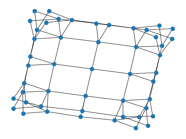
(b)

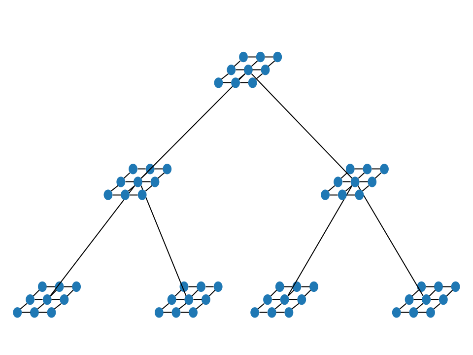
(c)

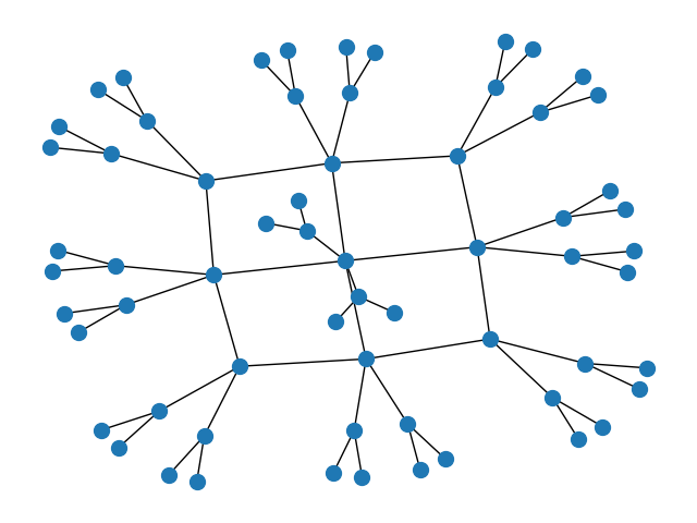
(d)

Figure 11: a) Cartesian product of tree and 2D grid. b) Cartesian product of tree and tree. c) Rooted product of tree and 2D grids. d) Rooted product of 2D grid and trees.

Retraction: Following Nickel & Kiela (2017) we experiment with a simple retraction:

$$\mathcal{R}_{\theta_{t}}(v)=\theta+v$$

C.3 Graph Reconstruction

Loss Function:

To compute the embeddings, we optimize the distance-based loss function proposed in Gu et al. (2019). Given graph distances $\{d_{G}(X_{i},X_{j})\}_{ij}$ between all pairs of connected nodes, the loss is defined as:

$$\mathcal{L}(x)=\sum_{1\leq i\leq j\leq n}\left|\left(\frac{d_{\mathcal{P}}(x_{i},x_{j})}{d_{G}(X_{i},X_{j})}\right)^{2}-1\right|$$

where $d_{\mathcal{P}}(x_{i},x_{j})$ is the distance between the corresponding node representations in the embeddings space. This formulation of the loss function captures the average distortion. We regard as future work experimenting with different loss functions, similar to the ones proposed on Cruceru et al. (2020).

Evaluation Metrics:

To measure the quality of the learned embeddings we follow the same fidelity metrics applied in Gu et al. (2019), which are distortion and precision. The distortion of a pair of connected nodes $a,b$ in the graph $G$, where $f(a),f(b)$ are their respective embeddings in the space $\mathcal{P}$ is given by:

$$\operatorname{distortion}(a,b)=\frac{|d_{\mathcal{P}}(f(a),f(b))-d_{G}(a,b)|}{d_{G}(a,b)}$$

The average distortion $D_{avg}$ is the average over all pairs of points. Distortion is a global metric that considers the explicit value of all distances.

The other metric that we consider is the mean average precision (mAP). It is a ranking-based measure for local neighborhoods that does not track explicit distances. Let $G=(V,E)$ be a graph and node $a\in V$ have neighborhood $\mathcal{N}_{a}=\{b_{1},...,b_{\operatorname{deg}(a)}\}$, where $\operatorname{deg}(a)$ is the degree of $a$. In the embedding $f$, define $R_{a,b_{i}}$ to be the smallest ball around $f(a)$ that contains $b_{i}$ (that is, $R_{a,b_{i}}$ is the smallest set of nearest points required to retrieve the $i$-th neighbor of $a$ in $f$). Then:

$$\operatorname{mAP}(f)=\frac{1}{|V|}\sum_{a\in V}\frac{1}{\operatorname{deg(a)}}\sum_{i=1}^{|\mathcal{N}_{a}|}\frac{|\mathcal{N}_{a}\cap R_{a,b_{i}}|}{|R_{a,b_{i}}|}$$

Data:

We employ NetworkX (Hagberg et al., 2008) to generate the synthetic datasets, and their Cartesian and rooted products. The statistics of the synthetic datasets reported in this work are presented in Table 9, and a diagram of the graphs can be seen in Figure 11.

The real-world datasets were downloaded from the Network Repository (Rossi & Ahmed, 2015). Stats are presented in Table 10.

By triples we mean the 3-tuple $(\textbf{u},\textbf{v},d(\textbf{u},\textbf{v}))$, where u, v represent connected nodes in the graph, and $d(\textbf{u,v})$ is the shortest distance between them.

Graph Nodes Edges Triples Grid Layout Tree Valency Tree Height 4D Grid 625 2000 195,000 $(5)^{4}$ Tree 364 363 66,066 3 5 Tree $\times$ Grid 496 1,224 122,760 $4\times 4$ 2 3 Tree $\times$ Tree 225 420 25,200 2 3 Tree $\diamond$ Grids 775 1,270 299,925 $5\times 5$ 2 4 Grid $\diamond$ Trees 775 790 299,925 $5\times 5$ 2 4

Table 9: Synthetic graph stats

Graph Nodes Edges Triples USCA312 312 48,516 48,516 bio-diseasome 516 1,188 132,870 csphd 1,025 1,043 524,800 road-euroroad 1,039 1,305 539,241 facebook 4,039 88,234 8,154,741

Table 10: Real-world graph stats

Setup Details:

For all models and datasets we run the same grid search and optimize the distortion loss, applying Rsgd. We report the average of $5$ runs in all cases. The implementation of all baselines are taken from Geoopt (Kochurov et al., 2020). We train for $3000$ epochs, reducing the learning rate by a factor of $5$ if the model does not improve the performance after $50$ epochs, and early stopping based on the average distortion if the model does not improve after $150$ epochs. We use the burn-in strategy (Nickel & Kiela, 2017; Cruceru et al., 2020) training with a 10 times smaller learning rate for the first 10 epochs. We experiment with learning rates from $\{0.05,0.01,0.005,0.001\}$, batch sizes from $\{512,1024,2048\}$ and max gradient norm from $\{10,50,250\}$.

Experimental Observations:

We noticed that for some combinations of hyper-parameters and datasets, the learning process for the Bounded domain model becomes unstable. Points eventually fall outside of the space, and need to be projected in every epoch. We did not observe this behavior on the Siegel model. We consider that these findings are in line with the ones reported on Nickel & Kiela (2018), where they observe that the Lorentz model, since it is unbounded, is more stable for gradient-based optimization than the Poincaré one.

C.4 Recommender Systems

Setup Details:

For all models and datasets we run the same grid search and optimize the Hinge loss from Equation 3, applying Rsgd. We report the average of $5$ runs in all cases. We train for $500$ epochs, reducing the learning rate by a factor of $5$ if the model does not improve the performance after $50$ epochs, and early stopping based on the dev set if the model does not improve after $150$ epochs. We use the burn-in strategy (Nickel & Kiela, 2017; Cruceru et al., 2020) training with a 10 times smaller learning rate for the first 10 epochs. We experiment with learning rates from $\{0.1,0.05,0.01,0.005,0.001\}$, batch sizes from $\{1024,2048\}$ and max gradient norm from $\{10,50,250\}$.

Data:

We provide a brief description of the datasets used in the recommender systems experiments.

• ml-1m and ml-100k: refers to the MovieLens datasets (Harper & Konstan, 2015).

• last.fm: Dataset of artist listening records from 1892 users (Cantador et al., 2011).

• meetup: dataset crawled from Meetup.com, where the goal is to recommend events to users (Pham et al., 2015). The dataset consists of the data from two regions, New York City (NYC) and state of California (CA), we only report results for NYC.

Stats for the datasets are presented in Table 11.

To generate evaluation splits, the penultimate and last item the user has interacted with are withheld as dev and test set respectively.

Dataset Users Items Interactions Density (%) ml-1m 6,040 3,706 1,000,209 4.47 ml-100k 943 1,682 100,000 6.30 last.fm 1,892 17,632 92,834 0.28 meetup-nyc 46,895 16,612 277,863 0.04

Table 11: Recommender system dataset stats

C.5 Node Classification

Setup Details:

In these experiments, for all datasets we use the cosine distance on the datapoints’ features to compute a complete input distance graph. We employ the available features and normalize them so that each attribute has mean zero and standard deviation one. Once we have a graph, we embed it in the exact same way than in the graph reconstruction task. Finally, we use the learned node embeddings as features to feed a logistic regression classifier

Matrix Mapping:

Since the node embeddings lie in different metric spaces, we apply the corresponding logarithmic map to obtain a ”flat” representation before classifying. For the Siegel upper half-space model of dimension $n$, we apply the following mapping. From each complex matrix embedding $Z=X+iY$ we stack the result of the following operations in matrix form as:

$$M=\begin{pmatrix}Y+XY^{-1}X&XY^{-1}\\ Y^{-1}X&Y^{-1}\\ \end{pmatrix}$$

where $M\in\mathbb{R}^{2n\times 2n}$. This mapping is the natural realisation of HypSPD_n as a totally geodesic submanifold of ${\rm SPD}_{2n}$. Since $M\in{\rm SPD}_{2n}$, finally we apply the LogEig map as proposed by Huang & Gool (2017), which yields a representation in a flat space. This operations results in new matrix of the form:

$$\operatorname{LogEig}(M)=\begin{pmatrix}U&V\\ V&-U\\ \end{pmatrix}$$

where $U,V\in Sym(n)$. The final step is to take the upper triangular from $U$ and $V$, and concatenate them as a vector of $n(n+1)$ dimensions.

This procedure is implemented for the Upper half-space. In the case of the Bounded domain model, we first map the points to the upper half-space with the Cayley transform.

Datasets:

All datasets were downloaded from the UCI Machine Learning Repository (Dua & Graff, 2017). Statistics about the datasets used are presented in Table 12.

Dataset	Nodes	Classes	Triples
Iris	150	3	11,175
Zoo	101	7	5,050
Glass	214	6	22,790

Table 12: Machine learning datasets used for node classification.

C.6 Learning the Weights for Finsler Distances

Both Finsler metrics $F_{1}$ and $F_{\infty}$ exhibit outstanding results in our experiments. However, there are significant differences in their relative performances depending on the target dataset. $F_{1}$ and $F_{\infty}$ are two metrics among many variants in the family of Finsler metrics. Thus, we propose an alternative of our Finslerian models, by learning weights for the summation of Algo 1, step 5, according to: $d^{F_{W}}(Z_{1},Z_{2}):\sum_{i=1}^{n}\left[\alpha_{i}\operatorname{log}(\nicefrac{{1+d_{i}}}{{1-d_{i}}})\right]$ where $\alpha_{i}\in\mathbb{R}$ are model parameters. The intuition behind this variant is to impose an inductive bias through the family of Finsler metrics, while allowing the model to learn from the data which particular metric is more suitable in each case. The model has flexibility to represent $F_{1}$ or $F_{\infty}$, and also explore different variations, such as Finsler metrics of minimum entropy (Boland & Newberger, 2001). We report results in Table 13. We observe that the model recovers the $F_{1}$ metric in the cases where it is the most convenient, whereas for Tree $\diamond$ Grids, it finds a more optimal solution.

4D Grid Tree $\times$ Tree Tree $\diamond$ Grids $D_{avg}$ mAP $D_{avg}$ mAP $D_{avg}$ mAP $\mathcal{S}_{4}^{F_{\infty}}$ 5.92 99.61 3.31 99.95 10.88 63.52 $\mathcal{S}_{4}^{F_{1}}$ 0.01 100.00 1.08 100.00 1.03 78.71 $\mathcal{S}_{4}^{F_{W}}$ 0.00 100.00 1.09 100.00 0.91 93.37

Table 13: Comparison with learning weights for Finsler metrics.

Appendix D Distance Algorithm Complexity

D.1 Theoretical Complexity

In this section we discuss the computational theoretical complexity of the different operations involved in the development of this work. We employ Big O notation. Since in all cases operations are not nested, but are applied sequentially, the costs can be added resulting in a polynomial expression. Thus, by applying the properties of the notation, we disregard lower-order terms of the polynomial.

Real Matrix Operations:

For $n\times n$ matrices with real entries, the associated complexity of each operation is as follows:

• Addition and subtraction: $\mathcal{O}(n^{2})$

• Multiplication: $\mathcal{O}(n^{2.4})$

• Inversion: $\mathcal{O}(n^{2.4})$

• Diagonalization: $\mathcal{O}(n^{3})$

Complex Matrix Operations:

A complex symmetric matrix $Z\in{\rm Sym}(n,\mathbb{C})$ can be written as $Z=X+iY$, where $X=\Re(Z),Y=\Im(Z)\in{\rm Sym}(n,\mathbb{R})$ are symmetric matrices with real entries. We implement the elemental operations for these matrices with the following associated costs:

• Multiplication: $\mathcal{O}(n^{2.4})$. It involves $4$ real matrix multiplications, plus additions and subtractions.

• Square root: $\mathcal{O}(n^{3})$. It involves a diagonalization and $2$ matrix multiplications.

• Inverse: $\mathcal{O}(n^{2.4})$. It involves real matrix inversions and multiplications (Falkenberg, 2007).

Takagi Factorization:

This factorization involves complex and real multiplications ($\mathcal{O}(n^{2.4})$), and diagonalizations ($\mathcal{O}(n^{3})$). It also involves the diagonalization of a $2nx2n$ matrix, which implies:

$$\mathcal{O}((2n)^{3})=\mathcal{O}(8n^{3})\simeq\mathcal{O}(n^{3})$$ (7)

Therefore, the final boundary for its cost is $\mathcal{O}(n^{3})$.

Cayley Transform:

This operation along with its inverse are composed of matrix inversions and multiplications, thus the cost is $\mathcal{O}(n^{2.4})$.

Distance Algorithm:

The full computation of the distance algorithm in the upperhalf space involves matrix square root, multiplications, inverses, and the application of the Cayley transform and the Takagi factorization. Since they are applied sequentially, without affecting the dimensionality of the matrices, we can take the highest value as the asymptotic cost of the algorithm, which is $\mathcal{O}(n^{3})$.

For the bounded domain, the matrices are mapped into the upperhalf space by an additional application of the inverse Cayley transform, and then the same distance algorithm is applied. Therefore, in this space the complexity also converges to $\mathcal{O}(n^{3})$.

D.2 Empirical Complexity

To empirically measure the time involved in the distance calculation we generate a batch of $1024$ pairs of points ($n\times n$ matrices). We perform the time evaluation for different values of $n$. Results can be observed in Figure 12.

We observe that as we increase the dimensionality, the relation tends to be polynomial, in line with the theoretical cost stated in §1.

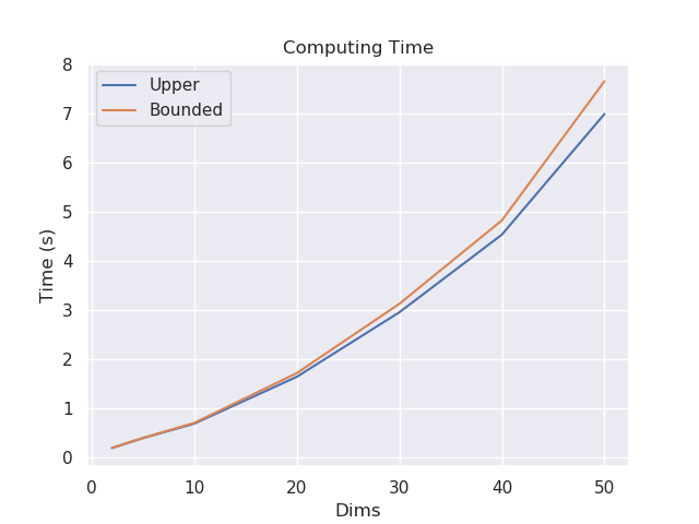
Figure 12: Time of distance calculation for a batch of $1024$ pairs of points for different matrix dimensions.

Appendix E Vector-valued Distance: a Tool for the Analysis of Embeddings

The vector-valued distance can also be used to develop other tools to analyze the embedding. More specifically we use it not only to create a continuous edge coloring as in Section 6, but also a vector distance plot, and a continuous node coloring with respect to a root.

For the vectorial distance plot we sample pairs of connected vertices of the graph $\{z_{i},z_{j}\}$ and plot the result of $\mathrm{vDist}(Z_{i},Z_{j})=(v_{1},v_{2})$ (see Algorithm 1, step $6$). In Figure 13-20 we show the plots of $(v_{1},v_{2})$ for the embeddings of different dataset embedded into the Upper Half models with respect to Riemannian, $F_{1}$ and $F_{\infty}$ metrics. In the $F_{1}$ case, the addition of both $d$-values sums up to the distance, whereas for the $F_{\infty}$, the largest $v$ ($v_{1}$) corresponds to the distance. The plots match the $\ell^{1}$ and $\ell^{\infty}$ metrics from Figure 2, verifying the intuition about the distances.

(a)

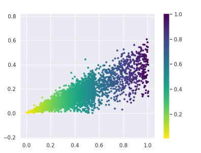
(b)

(c)

Figure 13: Plot of $(v_{1},v_{2})$ of $\mathcal{S}_{2}^{R}$ (left), $\mathcal{S}_{2}^{F1}$ (center), and $\mathcal{S}_{2}^{F_{\infty}}$ (right) for vertex pairs sampled from USCA312. Color indicates ground-truth distance.

(a)

(a)

The vectorial distance plots give a first qualitative visualization of the embedding. For dissimilar data sets, the edge plots look quite different. They can accumulate near the boundary of the cone (the diagonal or the horizontal), or be evenly distributed. The can also be refined by sampling only specific edges of the graph.

To construct a continuous node coloring we choose one vertex of our graph as the root $r$. For every other node $z$ we take the vector-valued distance from $r$ to $z$, and assign the ratio $\nicefrac{{v_{2}}}{{v_{1}}}$ as a value for this node. We again represent the corresponding real number by a color shading, as in Figures 21. It can be thought as the accumulated angle over a path from the root $r$ to the node $z$.

Evaluating the Quality of Embeddings: In the case of synthetic graphs, where we have full knowledge of the internal structure, we can use the edge and the node angles to compare the embeddings with respect to the Riemannian distance and the Finsler metrics $F_{1}$ and $F_{\infty}$. Illustrating this with the two dimensional grid, we observe in Figure 21 that while in the Finsler metric all edges have the same angle, the embedding optimizing the Riemannian distance is more distorted and less geodesics. In the case of the Finsler distances one can also see more clearly that the symmetries of the graph are respected in the embedding. This shows that the Finsler embeddings are much better in representing structural features of the graphs than the Riemannian embeddings.

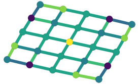
(a)

(b)

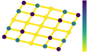
(c)

Figure 21: Analysis of $\mathcal{S}_{2}^{R}$ (left), $\mathcal{S}_{2}^{F_{\infty}}$ (center), and $\mathcal{S}_{2}^{F1}$ (right) for a $5\times 5$ grid. Node colors indicate the angle of the vector-valued distance by taking the path from the central node. Edge colors indicate the angle for each edge.

More Edge Coloring:

We plot the edge coloring for the three analyzed metric spaces, namely $\mathcal{S}_{2}^{R},\mathcal{S}_{2}^{F_{\infty}},\mathcal{S}_{2}^{F1}$ for the datasets analyzed in Figure 4, and for csphd in Figure 22-25. We can observe that in the Riemannian metric plots (left-hand side) there is no clear pattern that separates flat and hierarchical components in the graphs. The $F_{\infty}$ and $F1$ metrics are the best at capturing the structural aspect of the datasets. They recognize very similar patterns, though they assign opposite angles to the vector-valued distance vectors, and this can be noticed from the fact that the colors assigned are in opposite sides of the spectrum (yellow means angles close to zero, blue means angles close to 45°).

To plot these visualizations and the ones of Figure 5, we adapted code released by Cruceru et al. (2020).

(a)

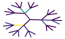
(b)

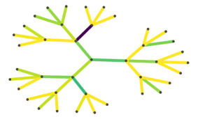
(c)

Figure 22: Edge coloring of $\mathcal{S}_{2}^{R}$ (left), $\mathcal{S}_{2}^{F_{\infty}}$ (center), and $\mathcal{S}_{2}^{F1}$ (right) for a tree.

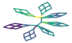
(a)

(b)

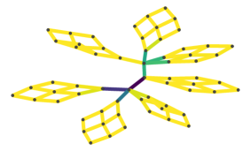
(c)

Figure 23: Edge coloring of $\mathcal{S}_{2}^{R}$ (left), $\mathcal{S}_{2}^{F_{\infty}}$ (center), and $\mathcal{S}_{2}^{F1}$ (right) for a tree $\diamond$ grids.

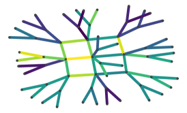
(a)

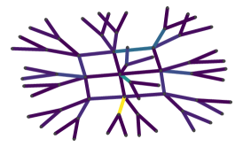
(b)

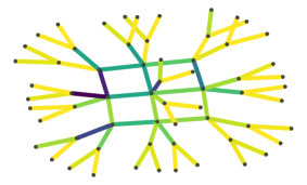
(c)

Figure 24: Edge coloring of $\mathcal{S}_{2}^{R}$ (left), $\mathcal{S}_{2}^{F_{\infty}}$ (center), and $\mathcal{S}_{2}^{F1}$ (right) for a grid $\diamond$ trees.

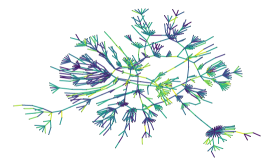
(a)

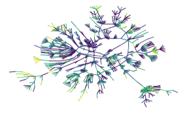
(b)

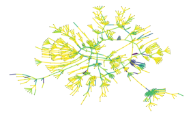
(c)

Figure 25: Edge coloring of $\mathcal{S}_{2}^{R}$ (left), $\mathcal{S}_{2}^{F_{\infty}}$ (center), and $\mathcal{S}_{2}^{F1}$ (right) for csphd.

Appendix F More Results

Results for graph reconstruction in lower dimensions are presented in Table 14

4D Grid Tree Tree $\times$ Grid Tree $\times$ Tree Tree $\diamond$ Grids Grid $\diamond$ Trees $(|V|,|E|)$ $(625,2000)$ $(364,363)$ $(496,1224)$ $(225,420)$ $(775,1270)$ $(775,790)$ $D_{avg}$ mAP $D_{avg}$ mAP $D_{avg}$ mAP $D_{avg}$ mAP $D_{avg}$ mAP $D_{avg}$ mAP $\mathbb{E}^{12}$ 11.24$\pm$0.00 100.00 5.71$\pm$0.01 32.72 9.80$\pm$0.00 83.25 9.79$\pm$0.00 95.97 5.11$\pm$0.05 22.24 5.48$\pm$0.03 21.84 $\mathbb{H}^{12}$ 25.23$\pm$0.06 63.86 2.09$\pm$0.28 97.32 17.12$\pm$0.00 83.29 20.55$\pm$0.12 75.98 14.12$\pm$0.45 44.06 14.76$\pm$0.23 31.96 $\mathbb{E}^{6}\times\mathbb{H}^{6}$ 11.24$\pm$0.00 100.00 1.61$\pm$0.07 100.00 9.20$\pm$0.03 100.00 9.34$\pm$0.05 98.14 2.53$\pm$0.07 58.86 2.38$\pm$0.04 97.56 $\mathbb{H}^{6}\times\mathbb{H}^{6}$ 18.76$\pm$0.02 79.05 0.92$\pm$0.04 99.95 12.92$\pm$0.86 89.71 9.71$\pm$2.47 96.82 1.32$\pm$0.08 72.62 3.10$\pm$0.62 86.40 $\mathcal{S}_{3}^{R}$ 13.26$\pm$0.01 99.54 1.69$\pm$0.03 71.64 9.26$\pm$0.01 99.57 8.80$\pm$0.21 97.47 1.82$\pm$0.07 64.52 2.27$\pm$0.18 79.10 $\mathcal{S}_{3}^{F_{\infty}}$ 11.82$\pm$0.03 98.71 1.35$\pm$0.39 99.35 7.98$\pm$0.66 99.47 3.97$\pm$0.34 99.64 13.01$\pm$0.64 55.89 11.26$\pm$0.59 68.30 $\mathcal{S}_{3}^{F_{1}}$ 6.41$\pm$0.00 100.00 1.07$\pm$0.04 74.98 2.02$\pm$0.02 100.00 1.84$\pm$0.02 100.00 1.43$\pm$0.01 65.90 1.45$\pm$0.05 81.25 $\mathcal{B}_{3}^{R}$ 13.29$\pm$0.17 99.54 1.63$\pm$0.06 70.70 10.04$\pm$0.03 92.20 9.10$\pm$0.10 96.78 4.71$\pm$0.15 65.04 5.68$\pm$0.37 89.19 $\mathcal{B}_{3}^{F_{\infty}}$ 12.45$\pm$0.18 97.70 2.59$\pm$0.34 98.94 10.33$\pm$0.47 93.58 4.74$\pm$0.00 96.66 11.33$\pm$0.10 65.07 10.39$\pm$0.15 79.43 $\mathcal{B}_{3}^{F_{1}}$ 6.41$\pm$0.00 100.00 1.13$\pm$0.03 79.21 2.02$\pm$0.00 100.00 1.92$\pm$0.07 100.00 1.51$\pm$0.06 71.07 1.51$\pm$0.00 83.64

Table 14: Results for synthetic datasets. All models have same number of free parameters. Lower $D_{avg}$ is better. Higher mAP is better.

References

- Bachmann et al. (2020) Bachmann, G., Bécigneul, G., and Ganea, O.-E. Constant curvature graph convolutional networks. In 37th International Conference on Machine Learning (ICML), 2020.
- Bécigneul & Ganea (2019) Bécigneul, G. and Ganea, O.-E. Riemannian adaptive optimization methods. In 7th International Conference on Learning Representations, ICLR, New Orleans, LA, USA, May 2019. URL https://openreview.net/forum?id=r1eiqi09K7.
- Boland & Newberger (2001) Boland, J. and Newberger, F. Minimal entropy rigidity for Finsler manifolds of negative flag curvature. Ergodic Theory and Dynamical Systems, 21(1):13–23, 2001. doi: 10.1017/S0143385701001055.
- Bonnabel (2011) Bonnabel, S. Stochastic gradient descent on Riemannian manifolds. IEEE Transactions on Automatic Control, 58, 11 2011. doi: 10.1109/TAC.2013.2254619.
- Bronstein et al. (2017) Bronstein, M. M., Bruna, J., LeCun, Y., Szlam, A., and Vandergheynst, P. Geometric deep learning: Going beyond Euclidean data. IEEE Signal Processing Magazine, 34(4):18–42, 2017.
- Cantador et al. (2011) Cantador, I., Brusilovsky, P., and Kuflik, T. 2nd Workshop on Information Heterogeneity and Fusion in Recommender Systems (HetRec 2011). In Proceedings of the 5th ACM Conference on Recommender Systems, RecSys 2011, New York, NY, USA, 2011. ACM.
- Cayley (1846) Cayley, A. Sur quelques propriétés des déterminants gauches. Journal für die reine und angewandte Mathematik, 32:119–123, 1846. URL http://www.digizeitschriften.de/dms/img/?PID=GDZPPN002145308.
- Chamberlain et al. (2017) Chamberlain, B., Deisenroth, M., and Clough, J. Neural embeddings of graphs in hyperbolic space. In Proceedings of the 13th International Workshop on Mining and Learning with Graphs (MLG), 2017.
- Chami et al. (2019) Chami, I., Ying, Z., Ré, C., and Leskovec, J. Hyperbolic graph convolutional neural networks. In Advances in Neural Information Processing Systems 32, pp. 4869–4880. Curran Associates, Inc., 2019. URL https://proceedings.neurips.cc/paper/2019/file/0415740eaa4d9decbc8da001d3fd805f-Paper.pdf.
- Chami et al. (2020) Chami, I., Gu, A., Chatziafratis, V., and Ré, C. From trees to continuous embeddings and back: Hyperbolic hierarchical clustering. In Larochelle, H., Ranzato, M., Hadsell, R., Balcan, M., and Lin, H. (eds.), Advances in Neural Information Processing Systems 33: Annual Conference on Neural Information Processing Systems 2020, NeurIPS 2020, December 6-12, 2020, virtual, 2020.
- Cruceru et al. (2020) Cruceru, C., Bécigneul, G., and Ganea, O.-E. Computationally tractable Riemannian manifolds for graph embeddings. In 37th International Conference on Machine Learning (ICML), 2020.
- Defferrard et al. (2020) Defferrard, M., Milani, M., Gusset, F., and Perraudin, N. DeepSphere: A graph-based spherical CNN. In International Conference on Learning Representations, 2020. URL https://openreview.net/forum?id=B1e3OlStPB.
- Donoho & Tsaig (2008) Donoho, D. L. and Tsaig, Y. Fast solution of -norm minimization problems when the solution may be sparse. IEEE Trans. Information Theory, 54(11):4789–4812, 2008.
- Dua & Graff (2017) Dua, D. and Graff, C. UCI machine learning repository, 2017. URL http://archive.ics.uci.edu/ml.
- Falkenberg (2007) Falkenberg, A. Method to calculate the inverse of a complex matrix using real matrix inversion. 2007.
- Ganea et al. (2018) Ganea, O.-E., Bécigneul, G., and Hofmann, T. Hyperbolic entailment cones for learning hierarchical embeddings. In Dy, J. and Krause, A. (eds.), Proceedings of the 35th International Conference on Machine Learning, volume 80 of Proceedings of Machine Learning Research, pp. 1646–1655, Stockholmsmässan, Stockholm Sweden, 10–15 Jul 2018. PMLR. URL http://proceedings.mlr.press/v80/ganea18a.html.
- Goh et al. (2007) Goh, K.-I., Cusick, M. E., Valle, D., Childs, B., Vidal, M., and Barabási, A.-L. The human disease network. Proceedings of the National Academy of Sciences, 104(21):8685–8690, 2007.
- Grattarola et al. (2020) Grattarola, D., Zambon, D., Livi, L., and Alippi, C. Change detection in graph streams by learning graph embeddings on constant-curvature manifolds. IEEE Trans. Neural Networks Learn. Syst., 31(6):1856–1869, 2020. doi: 10.1109/TNNLS.2019.2927301. URL https://doi.org/10.1109/TNNLS.2019.2927301.
- Gu et al. (2019) Gu, A., Sala, F., Gunel, B., and Ré, C. Learning mixed-curvature representations in product spaces. In International Conference on Learning Representations, 2019. URL https://openreview.net/forum?id=HJxeWnCcF7.
- Hagberg et al. (2008) Hagberg, A. A., Schult, D. A., and Swart, P. J. Exploring network structure, dynamics, and function using NetworkX. In Varoquaux, G., Vaught, T., and Millman, J. (eds.), Proceedings of the 7th Python in Science Conference, pp. 11 – 15, Pasadena, CA USA, 2008.
- Harper & Konstan (2015) Harper, F. M. and Konstan, J. A. The MovieLens datasets: History and context. ACM Trans. Interact. Intell. Syst., 5(4), December 2015. ISSN 2160-6455. doi: 10.1145/2827872. URL https://doi.org/10.1145/2827872.
- He et al. (2017) He, X., Liao, L., Zhang, H., Nie, L., Hu, X., and Chua, T.-S. Neural collaborative filtering. In Proceedings of the 26th International Conference on World Wide Web, WWW ’17, pp. 173–182, Republic and Canton of Geneva, CHE, 2017. International World Wide Web Conferences Steering Committee. ISBN 9781450349130. doi: 10.1145/3038912.3052569. URL https://doi.org/10.1145/3038912.3052569.
- Helgason (1978) Helgason, S. Differential geometry, Lie groups, and symmetric spaces. Academic Press New York, 1978. ISBN 0123384605.
- Hsieh et al. (2017) Hsieh, C.-K., Yang, L., Cui, Y., Lin, T.-Y., Belongie, S., and Estrin, D. Collaborative metric learning. In Proceedings of the 26th International Conference on World Wide Web, WWW ’17, pp. 193–201, Republic and Canton of Geneva, CHE, 2017. International World Wide Web Conferences Steering Committee. ISBN 9781450349130. doi: 10.1145/3038912.3052639. URL https://doi.org/10.1145/3038912.3052639.
- Huang & Gool (2017) Huang, Z. and Gool, L. V. A Riemannian network for SPD matrix learning. In Proceedings of the Thirty-First AAAI Conference on Artificial Intelligence, AAAI’17, pp. 2036–2042. AAAI Press, 2017.
- Huang et al. (2018) Huang, Z., Wu, J., and Gool, L. V. Building deep networks on Grassmann manifolds. In McIlraith, S. A. and Weinberger, K. Q. (eds.), Proceedings of the Thirty-Second AAAI Conference on Artificial Intelligence, (AAAI-18), the 30th Innovative Applications of Artificial Intelligence (IAAI-18), and the 8th AAAI Symposium on Educational Advances in Artificial Intelligence (EAAI-18), New Orleans, Louisiana, USA, February 2-7, 2018, pp. 3279–3286. AAAI Press, 2018. URL https://www.aaai.org/ocs/index.php/AAAI/AAAI18/paper/view/16846.
- Kochurov et al. (2020) Kochurov, M., Karimov, R., and Kozlukov, S. Geoopt: Riemannian optimization in PyTorch. ArXiv, abs/2005.02819, 2020.
- Krioukov et al. (2009) Krioukov, D., Papadopoulos, F., Vahdat, A., and Boguñá, M. On Curvature and Temperature of Complex Networks. Physical Review E, 80(035101), Sep 2009.
- Krioukov et al. (2010) Krioukov, D., Papadopoulos, F., Kitsak, M., Vahdat, A., and Boguñá, M. Hyperbolic geometry of complex networks. Physical review. E, Statistical, nonlinear, and soft matter physics, 82:036106, 09 2010. doi: 10.1103/PhysRevE.82.036106.
- Law & Stam (2020) Law, M. T. and Stam, J. Ultrahyperbolic representation learning. In Larochelle, H., Ranzato, M., Hadsell, R., Balcan, M., and Lin, H. (eds.), Advances in Neural Information Processing Systems 33: Annual Conference on Neural Information Processing Systems 2020, NeurIPS 2020, December 6-12, 2020, virtual, 2020.
- Liu et al. (2017) Liu, W., Wen, Y., Yu, Z., Li, M., Raj, B., and Song, L. SphereFace: Deep hypersphere embedding for face recognition. In 2017 IEEE Conference on Computer Vision and Pattern Recognition (CVPR), pp. 6738–6746, 2017. doi: 10.1109/CVPR.2017.713.
- López & Strube (2020) López, F. and Strube, M. A fully hyperbolic neural model for hierarchical multi-class classification. In Findings of the Association for Computational Linguistics: EMNLP 2020, pp. 460–475, Online, November 2020. Association for Computational Linguistics. URL https://www.aclweb.org/anthology/2020.findings-emnlp.42.
- López et al. (2019) López, F., Heinzerling, B., and Strube, M. Fine-grained entity typing in hyperbolic space. In Proceedings of the 4th Workshop on Representation Learning for NLP (RepL4NLP-2019), pp. 169–180, Florence, Italy, August 2019. Association for Computational Linguistics. doi: 10.18653/v1/W19-4319. URL https://www.aclweb.org/anthology/W19-4319.
- McAuley & Leskovec (2012) McAuley, J. and Leskovec, J. Learning to discover social circles in ego networks. In Proceedings of the 25th International Conference on Neural Information Processing Systems - Volume 1, NIPS’12, pp. 539–547, Red Hook, NY, USA, 2012. Curran Associates Inc.
- Meng et al. (2019) Meng, Y., Huang, J., Wang, G., Zhang, C., Zhuang, H., Kaplan, L., and Han, J. Spherical text embedding. In Wallach, H., Larochelle, H., Beygelzimer, A., d'Alché-Buc, F., Fox, E., and Garnett, R. (eds.), Advances in Neural Information Processing Systems, volume 32, pp. 8208–8217. Curran Associates, Inc., 2019. URL https://proceedings.neurips.cc/paper/2019/file/043ab21fc5a1607b381ac3896176dac6-Paper.pdf.
- Nickel & Kiela (2017) Nickel, M. and Kiela, D. Poincaré embeddings for learning hierarchical representations. In Guyon, I., Luxburg, U. V., Bengio, S., Wallach, H., Fergus, R., Vishwanathan, S., and Garnett, R. (eds.), Advances in Neural Information Processing Systems 30, pp. 6341–6350. Curran Associates, Inc., 2017. URL https://proceedings.neurips.cc/paper/2017/file/59dfa2df42d9e3d41f5b02bfc32229dd-Paper.pdf.
- Nickel & Kiela (2018) Nickel, M. and Kiela, D. Learning continuous hierarchies in the Lorentz model of hyperbolic geometry. In Dy, J. and Krause, A. (eds.), Proceedings of the 35th International Conference on Machine Learning, volume 80 of Proceedings of Machine Learning Research, pp. 3779–3788, Stockholmsmässan, Stockholm Sweden, 10–15 Jul 2018. PMLR. URL http://proceedings.mlr.press/v80/nickel18a.html.
- Nielsen & Sun (2019) Nielsen, F. and Sun, K. Clustering in Hilbert’s Projective Geometry: The Case Studies of the Probability Simplex and the Elliptope of Correlation Matrices, pp. 297–331. Springer International Publishing, Cham, 2019. ISBN 978-3-030-02520-5. doi: 10.1007/978-3-030-02520-5˙11. URL https://doi.org/10.1007/978-3-030-02520-5_11.
- Nooy et al. (2011) Nooy, W. D., Mrvar, A., and Batagelj, V. Exploratory Social Network Analysis with Pajek. Cambridge University Press, USA, 2011. ISBN 0521174805.
- Paszke et al. (2019) Paszke, A., Gross, S., Massa, F., Lerer, A., Bradbury, J., Chanan, G., Killeen, T., Lin, Z., Gimelshein, N., Antiga, L., Desmaison, A., Kopf, A., Yang, E., DeVito, Z., Raison, M., Tejani, A., Chilamkurthy, S., Steiner, B., Fang, L., Bai, J., and Chintala, S. Pytorch: An imperative style, high-performance deep learning library. In Wallach, H., Larochelle, H., Beygelzimer, A., d'Alché-Buc, F., Fox, E., and Garnett, R. (eds.), Advances in Neural Information Processing Systems 32, pp. 8024–8035. Curran Associates, Inc., 2019.
- Pennec (2020) Pennec, X. Manifold-Valued Image Processing with SDP Matrices. In Riemannian Geometric Statistics in Medical Image Analysis, pp. 75–134. Academic Press, 2020.
- Pham et al. (2015) Pham, T. N., Li, X., Cong, G., and Zhang, Z. A general graph-based model for recommendation in event-based social networks. In 2015 IEEE 31st International Conference on Data Engineering, pp. 567–578, 2015. doi: 10.1109/ICDE.2015.7113315.
- Ratliff et al. (2020) Ratliff, N. D., Wyk, K. V., Xie, M., Li, A., and Rana, M. A. Generalized nonlinear and Finsler geometry for robotics. CoRR, abs/2010.14745, 2020. URL https://arxiv.org/abs/2010.14745.
- Rossi & Ahmed (2015) Rossi, R. A. and Ahmed, N. K. The network data repository with interactive graph analytics and visualization. In AAAI, 2015. URL http://networkrepository.com.
- Rubin-Delanchy (2020) Rubin-Delanchy, P. Manifold structure in graph embeddings, 2020. URL https://arxiv.org/abs/2006.05168.
- Sala et al. (2018) Sala, F., De Sa, C., Gu, A., and Re, C. Representation tradeoffs for hyperbolic embeddings. In Dy, J. and Krause, A. (eds.), Proceedings of the 35th International Conference on Machine Learning, volume 80 of Proceedings of Machine Learning Research, pp. 4460–4469, Stockholmsmässan, Stockholm Sweden, 10–15 Jul 2018. PMLR. URL http://proceedings.mlr.press/v80/sala18a.html.
- Siegel (1943) Siegel, C. L. Symplectic geometry. American Journal of Mathematics, 65(1):1–86, 1943. ISSN 00029327, 10806377. URL http://www.jstor.org/stable/2371774.
- Skopek et al. (2020) Skopek, O., Ganea, O.-E., and Becigneul, G. Mixed-curvature variational autoencoders. In 8th International Conference on Learning Representations (ICLR), April 2020. URL https://openreview.net/pdf?id=S1g6xeSKDS.
- Takagi (1924) Takagi, T. On an algebraic problem related to an analytic theorem of carathéodory and fejér and on an allied theorem of Landau. Japanese journal of mathematics :transactions and abstracts, 1:83–93, 1924. doi: 10.4099/jjm1924.1.0˙83.
- Tifrea et al. (2019) Tifrea, A., Bécigneul, G., and Ganea, O.-E. Poincare GloVe: Hyperbolic word embeddings. In 7th International Conference on Learning Representations, ICLR, New Orleans, LA, USA, May 2019. URL https://openreview.net/forum?id=Ske5r3AqK7.
- Vinh Tran et al. (2020) Vinh Tran, L., Tay, Y., Zhang, S., Cong, G., and Li, X. HyperML: A boosting metric learning approach in hyperbolic space for recommender systems. In Proceedings of the 13th International Conference on Web Search and Data Mining, WSDM ’20, pp. 609–617, New York, NY, USA, 2020. Association for Computing Machinery. ISBN 9781450368223. doi: 10.1145/3336191.3371850. URL https://doi.org/10.1145/3336191.3371850.
- Wilson et al. (2014) Wilson, R. C., Hancock, E. R., Pekalska, E., and Duin, R. P. W. Spherical and hyperbolic embeddings of data. IEEE Transactions on Pattern Analysis and Machine Intelligence, 36(11):2255–2269, 2014.
- Xu & Durrett (2018) Xu, J. and Durrett, G. Spherical latent spaces for stable variational autoencoders. In Proceedings of the 2018 Conference on Empirical Methods in Natural Language Processing, 2018.