Nonintegrability of the restricted three-body problem

Abstract.

The problem of nonintegrability of the circular restricted three-body problem is very classical and important in the theory of dynamical systems. It was partially solved by Poincaré in the nineteenth century: He showed that there exists no real-analytic first integral which depends analytically on the mass ratio of the second body to the first one and is functionally independent of the Hamiltonian. When the mass of the second body becomes zero, the restricted three-body problem reduces to the two-body Kepler problem. We prove the nonintegrability of the restricted three-body problem both in the planar and spatial cases for any nonzero mass of the second body. Our basic tool of the proofs is a technique developed here for determining whether perturbations of integrable systems which may be non-Hamiltonian are not meromorphically integrable near resonant periodic orbits such that the first integrals and commutative vector fields also depend meromorphically on the perturbation parameter. The technique is based on generalized versions due to Ayoul and Zung of the Morales-Ramis and Morales-Ramis-Simó theories.

1. Introduction

Figure 1. Configuration of the circular restricted three-body problem in the rotational frame.

In this paper we study the nonintegrability of the circular restricted three-body problem for the planar case,

$$\begin{split}&\dot{x}=p_{x}+y,\quad\dot{p}_{x}=p_{y}+\frac{\partial U_{2}}{\partial x}(x,y),\\ &\dot{y}=p_{y}-x,\quad\dot{p}_{y}=-p_{x}+\frac{\partial U_{2}}{\partial y}(x,y),\end{split}$$ (1.1)

and for the spatial case,

$$\begin{split}&\dot{x}=p_{x}+y,\quad\dot{p}_{x}=p_{y}+\frac{\partial U_{3}}{\partial x}(x,y,z),\\ &\dot{y}=p_{y}-x,\quad\dot{p}_{y}=-p_{x}+\frac{\partial U_{3}}{\partial y}(x,y,z),\\ &\dot{z}=p_{z},\quad\dot{p}_{z}=\frac{\partial U_{3}}{\partial z}(x,y,z),\end{split}$$ (1.2)

where

$$U_{2}(x,y)=\frac{\mu}{\sqrt{(x-1+\mu)^{2}+y^{2}}}+\frac{1-\mu}{\sqrt{(x+\mu)^{2}+y^{2}}},$$

$$U_{3}(x,y,z)=\frac{\mu}{\sqrt{(x-1+\mu)^{2}+y^{2}+z^{2}}}+\frac{1-\mu}{\sqrt{(x+\mu)^{2}+y^{2}+z^{2}}}.$$

The systems (1.1) and (1.2) are Hamiltonian with the Hamiltonians

$$H_{2}(x,y,p_{x},p_{y})=\tfrac{1}{2}(p_{x}^{2}+p_{y}^{2})+(p_{x}y-p_{y}x)-U_{2}(x,y)$$

and

$$H_{3}(x,y,z,p_{x},p_{y},p_{z})=\tfrac{1}{2}(p_{x}^{2}+p_{y}^{2}+p_{z}^{2})+(p_{x}y-p_{y}x)-U_{3}(x,y,z),$$

respectively, and represent the dimensionless equations of motion of the third massless body subjected to the gravitational forces from the two primary bodies with mass $\mu$ and $1-\mu$ which remain at $(1-\mu,0)$ and $(-\mu,0)$, respectively, on the $xy$-plane in the rotational frame, under the assumption that the primaries rotate counterclockwise on the circles about their common center of mass at the origin in the inertial coordinate frame. See Fig. 1. Their nonintegarbllity means that Eq. (1.1) (resp. Eq. (1.2)) does not have one first integral (resp. two first integrals) which is (resp. are) functionally independent of the Hamiltonian $H_{2}$ (resp. $H_{3}$). See [3, 20] for the definition of integrability of general Hamiltonian systems, and, e.g., Section 4.1 of [19] for more details on the derivation and physical meaning of (1.1) and (1.2).

The problem of nonintegrability of (1.1) and (1.2) is very classical and important in the theory of dynamical systems. In his famous memoir [28], which was related to a prize competition celebrating the 60th birthday of King Oscar II, Henri Poincaré studied the planar case and discussed the nonexistsnce of a first integral which is analytic in the state variables and parameter $\mu$ near $\mu=0$ and functionally independent of the Hamiltonian. His approach was improved significantly in the first volume of his masterpieces [29] published two years later: he showed the nonexistence of such a first integral for the restricted three-body problem in the spatial case as well as the planar one. See [6] for an account of his work from mathematical and historical perspectives. His result was also explained in [4, 14, 15, 37]. Moreover, a remarkable progress has been made on the planar problem (1.1) in a different direction recently: Guardia et al. [12] showed the occurrence of transverse intersection between the stable and unstable manifolds of the infinity for any $\mu\in(0,1)$ in a region far from the primaries in which $r=\sqrt{x^{2}+y^{2}}$ and its conjugate momentum are sufficiently large. This implies, e.g., by Theorem 3.10 of [26], the real-analytic nonintetgrabilty of (1.1) as well as the existence of oscillatory motions such that $\limsup_{t\to\infty}r(t)=\infty$ while $\liminf_{t\to\infty}r(t)<\infty$. Similar results were obtained much earlier when $\mu>0$ is sufficiently small in [16] and for any $\mu\in(0,1)$ except for a certain finite number of the values in [39]. Note that these results immediately say nothing about the nonintegrability of the spatial problem (1.2).

On the other hand, the nonintegrability of the general three-body problem is now well understood, in comparison with the restricted one. Tsygvintsev [32, 33] proved the nonintegrability of the general planar three-body problem near the Lagrangian parabolic orbits in which the three bodies form an equilateral triangle and move along certain parabolas, using Ziglin’s method [44]. Boucher and Weil [9] also obtained a similar result, using the Morales-Ramis theory [20, 22], which is considered as an extension of the Ziglin method, while it was proven for the case of equal masses a little earlier in [8]. Moreover, Tsygvintsev [34, 35, 36] proved the nonexistence of a single additional first integral near the Lagrangian parabolic orbits when

$$\frac{m_{1}m_{2}+m_{2}m_{3}+m_{3}m_{1}}{(m_{1}+m_{2}+m_{3})^{2}}\notin\{\tfrac{7}{48},\tfrac{5}{16}\},$$

where $m_{j}$ represents the mass of the $j$th body for $j=1,2,3$. Subsequently, Morales-Ruiz and Simon [25] succeeded in removing the three exceptional cases and extended the result to the space of three or more dimensions. Ziglin [45] also proved the nonintegrability of the general three-body problem near a collinear solution which was used by Yoshida [42] for the problem in the one-dimensional space much earlier, in the space of any dimension when two of the three masses, say $m_{1},m_{2}$, are nearly equal but neither $m_{3}/m_{1}$ nor $m_{3}/m_{2}\in\{11/12,1/4,1/24\}$. Maciejewski and Przybylska [17] discussed the three-body problem with general homogeneous potentials. It should be noted that Ziglin [45] and Morales-Ruiz and Simon [25] also discussed the general $N$-body problem. We remark that these results say nothing about the nonintegrability of the restricted three-body problem obtained by limiting manipulation from the general one. In particular, there exists no nonconstant solution corresponding to the Lagrangian parabolic orbits or collinear solutions in the restricted one.

Here we show the nonintegrability of the three-body problems (1.1) and (1.2) near the primaries for any $\mu\in(0,1)$ fixed. To state our result precisely, we use the following treatment originally made in [10]. We first introduce the new variables $u_{1},u_{2}\in\mathbb{C}$ given by

$$u_{1}^{2}-(x-1+\mu)^{2}-y^{2}=0,\quad u_{2}^{2}-(x+\mu)^{2}-y^{2}=0$$

and

$$u_{1}^{2}-(x-1+\mu)^{2}-y^{2}-z^{2}=0,\quad u_{2}^{2}-(x+\mu)^{2}-y^{2}-z^{2}=0$$

and regard (1.1) and (1.2) as Hamiltonian systems on the four- and six-dimensional complex manifolds (algebraic varieties)

$$\mathscr{S}_{2}= \{(x,y,p_{x},p_{y},u_{1},u_{2})\in\mathbb{C}^{6}$$

$$\quad\mid u_{1}^{2}-(x-1+\mu)^{2}-y^{2}=u_{2}-(x+\mu)^{2}-y^{2}=0\}$$

and

$$\mathscr{S}_{3}= \{(x,y,z,p_{x},p_{y},p_{z},u_{1},u_{2})\in\mathbb{C}^{8}$$

$$\quad\mid u_{1}^{2}-(x-1+\mu)^{2}-y^{2}-z^{2}=u_{2}-(x+\mu)^{2}-y^{2}-z^{2}=0\},$$

respectively. Let $\pi_{2}:\mathscr{S}_{2}\to\mathbb{C}^{4}$ and $\pi_{3}:\mathscr{S}_{3}\to\mathbb{C}^{6}$ be the projections such that

$$\pi_{2}(x,y,p_{x},p_{y},u_{1},u_{2})=(x,y,p_{x},p_{y})$$

and

$$\pi_{3}(x,y,z,p_{x},p_{y},p_{z},u_{1},u_{2})=(x,y,z,p_{x},p_{y},p_{z}),$$

and let

$$\Sigma(\mathscr{S}_{2})= \{u_{1}=(x-1+\mu)^{2}+y^{2}=0\}$$

$$\quad\cup\{u_{2}=(x+\mu)^{2}+y^{2}=0\}\subset\mathscr{S}_{2},$$

$$\Sigma(\mathscr{S}_{3})= \{u_{1}=(x-1+\mu)^{2}+y^{2}+z^{2}=0\}$$

$$\quad\cup\{u_{2}=(x+\mu)^{2}+y^{2}+z^{2}=0\}\subset\mathscr{S}_{3}.$$

Note that $\pi_{2}$ and $\pi_{3}$ are singular on $\Sigma(\mathscr{S}_{2})$ and $\Sigma(\mathscr{S}_{3})$, respectively. The sets $\Sigma(\mathscr{S}_{2})$ and $\Sigma(\mathscr{S}_{3})$ are called the critical sets of $\mathscr{S}_{2}$ and $\mathscr{S}_{3}$, respectively. The systems (1.1) and (1.2) are, respectively, rewritten as

$$\begin{split}&\dot{x}=p_{x}+y,\quad\dot{p}_{x}=p_{y}-\frac{\mu}{w_{1}^{3}}(x-1+\mu),\\ &\dot{y}=p_{y}-x,\quad\dot{p}_{y}=-p_{x}-\frac{\mu}{w_{1}^{3}}y,\\ &\dot{u}_{1}=\frac{1}{u_{1}}((x-1+\mu)(p_{x}+y)+y(p_{y}-x),\\ &\dot{u}_{2}=\frac{1}{u_{2}}(x+\mu)(p_{x}+y)+y(p_{y}-x)\end{split}$$ (1.3)

and

$$\begin{split}&\dot{x}=p_{x}+y,\quad\dot{p}_{x}=p_{y}-\frac{\mu}{w_{1}^{3}}(x-1+\mu),\\ &\dot{y}=p_{y}-x,\quad\dot{p}_{y}=-p_{x}-\frac{\mu}{w_{1}^{3}}y,\\ &\dot{z}=p_{z},\quad\dot{p}_{z}=-\frac{\mu}{w_{1}^{3}}z,\\ &\dot{u}_{1}=\frac{1}{u_{1}}((x-1+\mu)(p_{x}+y)+y(p_{y}-x),\\ &\dot{u}_{2}=\frac{1}{u_{2}}(x+\mu)(p_{x}+y)+y(p_{y}-x)\end{split}$$ (1.4)

which are meromorphic on $\mathscr{S}_{2}$ and $\mathscr{S}_{3}$. We prove the following theorem.

Theorem 1.1.

The circular restricted three-body problem (1.1) $($resp. (1.2)$)$ does not have a complete set of first integrals in involution that are functionally independent almost everywhere and meromorphic in $(x,y,p_{x},p_{y},u_{1},u_{2})$ $($resp. in $(x,y,z,p_{x},p_{y},p_{z},u_{1},u_{2}))$ except on $\pi_{2}(\mathscr{S}_{2})$ $($resp. on $\pi_{3}(\mathscr{S}_{3}))$ in punctured neighborhoods of

$$(x,y)=(-\mu,0)\mbox{ and }(1-\mu,0)$$

$$(\mbox{resp.}\ (x,y,z)=(-\mu,0,0)\mbox{ and }(1-\mu,0,0))$$

for any $\mu\in(0,1)$, as Hamiltonian systems on $\mathscr{S}_{2}$ $($resp. on $\mathscr{S}_{3})$.

Proofs of Theorem 1.1 are given in Section 3 for the planar case (1.1) and in Section 4 for the spatial case (1.2). Our basic tool of the proofs is a technique developed in Section 2 for

$$\dot{I}=\varepsilon h(I,\theta;\varepsilon),\quad\dot{\theta}=\omega(I)+\varepsilon g(I,\theta;\varepsilon),\quad(I,\theta)\in\mathbb{R}^{\ell}\times\mathbb{T}^{m},$$ (1.5)

where $\ell,m\in\mathbb{N}$, $\mathbb{T}^{m}=(\mathbb{R}/2\pi\mathbb{Z})^{m}$, $\varepsilon$ is a small parameter such that $0<|\varepsilon|\ll 1$, and $\omega:\mathbb{R}^{\ell}\to\mathbb{R}^{m}$, $h:\mathbb{R}^{\ell}\times\mathbb{T}^{m}\times\mathbb{R}\to\mathbb{R}^{\ell}$ and $g:\mathbb{R}^{\ell}\times\mathbb{T}^{m}\times\mathbb{R}\to\mathbb{R}^{m}$ are meromorphic in their arguments. The system (1.5) is Hamiltonian if $\varepsilon=0$ or

$$\mathrm{D}_{I}h(I,\theta;\varepsilon)\equiv-\mathrm{D}_{\theta}g(I,\theta;\varepsilon)$$

as well as $\ell=m$, and non-Hamiltonian if not. The developed technique enables us to determine whether the system (1.5) is not meromorphically integrable in the Bogoyavlenskij sense [7] (see Definition 1.2 below) such that the first integrals and commutative vector fields also depend meromorphically on $\varepsilon$ near $\varepsilon=0$, like the result of Poincaré [28, 29] stated above, when the domains of the independent and dependent variables are extended to regions in $\mathbb{C}$ and $\mathbb{C}^{\ell}\times(\mathbb{C}/2\pi\mathbb{Z})^{m}$, respectively. The definition of integrability adopted here is precisely as follows.

Definition 1.2 (Bogoyavlenskij).

For $n\in\mathbb{N}$ an $n$-dimensional dynamical system

$$\dot{x}=f(x),\quad\mbox{$x\in\mathbb{R}^{n}$ or $\mathbb{C}^{n}$},$$

is called $(q,n-q)$-integrable or simply integrable if there exist $q$ vector fields $f_{1}(x)(:=f(x)),f_{2}(x),\dots,f_{q}(x)$ and $n-q$ scalar-valued functions $F_{1}(x),\dots,F_{n-q}(x)$ such that the following two conditions hold:

1. $f_{1}(x),\dots,f_{q}(x)$ are linearly independent almost everywhere and commute with each other, i.e., $[f_{j},f_{k}](x):=\mathrm{D}f_{k}(x)f_{j}(x)-\mathrm{D}f_{j}(x)f_{k}(x)\equiv 0$ for $j,k=1,\ldots,q$, where $[\cdot,\cdot]$ denotes the Lie bracket;

2. The derivatives $\mathrm{D}F_{1}(x),\dots,\mathrm{D}F_{n-q}(x)$ are linearly independent almost everywhere and $F_{1}(x),\dots,F_{n-q}(x)$ are first integrals of $f_{1},\dots,f_{q}$, i.e., $\mathrm{D}F_{k}(x)\cdot f_{j}(x)\equiv 0$ for $j=1,\ldots,q$ and $k=1,\ldots,n-q$, where “$\cdot$” represents the inner product.

We say that the system is meromorphically integrable if the first integrals and commutative vector fields are meromorphic.

Definition 1.2 is considered as a generalization of Liouville-integrability for Hamiltonian systems [3, 20] since an $n$-degree-of-freedom Liouville-integrable Hamiltonian system with $n\geq 1$ has not only $n$ functionally independent first integrals but also $n$ linearly independent commutative (Hamiltonian) vector fields generated by the first integrals. When $\varepsilon=0$, the system (1.5) is meromorphically $(m,\ell)$-integrable in the Bogoyavlenskij sense: $F_{j}(I,\theta)=I_{j}$, $j=1,\ldots,\ell$, are first integrals and $f_{j}(I,\theta)=(0,e_{j})\in\mathbb{R}^{\ell}\times\mathbb{R}^{m}$, $j=2,\ldots,m$, give $m$ commutative vector fields along with its own vector field, where $e_{j}$ is the $m$-dimensional vector of which the $j$th element is the unit and the other elements are zero. Conversely, a general $(m,\ell)$-integrable system is transformed to the form (1.5) with $\varepsilon=0$ if the level set of the first integrals $F_{1}(x),\ldots,F_{m}(x)$ has a connected compact component. See [7, 46] for more details. Thus, the system (1.5) can be regarded as a normal form for perturbations of general $(m,\ell)$-integrable systems.

Systems of the form (1.5) have attracted much attention, especially when they are Hamiltonian. See [3, 4, 15] and references therein for more details. In particular, Kozlov [15] extended the famous result of Poincaré [28, 29] for Hamiltonian systems to the general analytic case of (1.5) and gave sufficient conditions for nonexistence of additional real-analytic first integrals depending analytically on $\varepsilon$ near $\varepsilon=0$. See also [4, 14] for his result in Hamiltonian systems. Moreover, Motonaga and Yagasaki [27] gave sufficient conditions for real-analytic nonintegrability of general nearly integrable systems in the Bogoyavlenskij sense such that the first integrals and commutative vector fields also depend real-analytically on $\varepsilon$ near $\varepsilon=0$. The technique developed in Section 2 is different from them and based on a generalized version due to Ayoul and Zung [5] of the Morales-Ramis theory [20, 22]. See Appendix A of [40] for a brief review of the previous results and their comparison with the developed technique. The systems (1.1) and (1.2) are transformed to the form (1.5) in the punctured neighborhoods and the technique is applied to them.

2. Determination of nonintegrability for (1.5)

In this section, we give a technique for determining whether the system (1.5) is not meromorphically Bogoyavlenskij-integrable such that the first integrals and commutative vector fields also depend meromorphically on $\varepsilon$ near $\varepsilon=0$.

Figure 2. Assumption (A2).

When $\varepsilon=0$, Eq. (1.5) becomes

$$\dot{I}=0,\quad\dot{\theta}=\omega(I).$$ (2.1)

We assume the following on the unperturbed system (2.1):

1. For some $I^{\ast}\in\mathbb{R}^{\ell}$, a resonance of multiplicity $m-1$,

   $$\dim_{\mathbb{Q}}\langle\omega_{1}(I^{\ast}),\ldots,\omega_{m}(I^{\ast})\rangle=1,$$

   occurs with $\omega(I^{\ast})\neq 0$, i.e., there exists a constant $\omega^{\ast}>0$ such that

   $$\frac{\omega(I^{\ast})}{\omega^{\ast}}\in\mathbb{Z}^{m}\setminus\{0\},$$

   where $\omega_{j}(I)$ is the $j$th element of $\omega(I)$ for $j=1,\ldots,m$.

Note that we can replace $\omega^{\ast}$ with $\omega^{\ast}/n$ for any $n\in\mathbb{N}$ in (A1). We refer to the $m$-dimensional torus $\mathscr{T}^{\ast}=\{(I^{\ast},\theta)\mid\theta\in\mathbb{T}^{m}\}$ as the resonant torus and to periodic orbits $(I,\theta)=(I^{\ast},\omega(I^{\ast})t+\theta_{0})$, $\theta_{0}\in\mathbb{T}^{m}$, on $\mathscr{T}^{\ast}$ as the resonant periodic orbits. Let $T^{\ast}=2\pi/\omega^{\ast}$. We also make the following assumption.

1. For some $k\in\mathbb{Z}_{\geq 0}:=\mathbb{N}\cup\{0\}$ and $\theta\in\mathbb{T}^{m}$ there exists a closed loop $\gamma_{\theta}$ in a region including $(0,T^{\ast})\subset\mathbb{R}$ in $\mathbb{C}$ such that $\gamma_{\theta}\cap(i\mathbb{R}\cup(T^{\ast}+i\mathbb{R}))=\emptyset$ and

   $$\mathscr{I}^{k}(\theta):=\frac{1}{k!}\mathrm{D}\omega(I^{\ast})\int_{\gamma_{\theta}}\mathrm{D}_{\varepsilon}^{k}h(I^{\ast},\omega(I^{\ast})\tau+\theta;0)\mathrm{d}\tau$$ (2.2)

   is not zero. See Fig. 2

Note that the condition $\gamma_{\theta}\cap(i\mathbb{R}\cup(T^{\ast}+i\mathbb{R}))=\emptyset$ is not essential in (A2), since it always holds by replacing $\omega^{\ast}$ with $\omega^{\ast}/n$ for sufficiently large $n\in\mathbb{N}$ if necessary. We prove the following theorem which guarantees that conditions (A1) and (A2) are sufficient for nonintegrability of (1.5) in a certain meaning.

Theorem 2.1.

Let $\Gamma$ be any domain in $\mathbb{C}/T^{\ast}\mathbb{Z}$ containing $\mathbb{R}/T^{\ast}\mathbb{Z}$ and $\gamma_{\theta}$. Suppose that assumption (A1) and (A2) hold for some $\theta=\theta_{0}\in\mathbb{T}^{m}$. Then the system (1.5) is not meromorphically integrable in the Bogoyavlenskij sense near the resonant periodic orbit $(I,\theta)=(I^{\ast},\omega(I^{\ast})\tau+\theta_{0})$ with $\tau\in\Gamma$ such that the first integrals and commutative vector fields also depend meromorphically on $\varepsilon$ near $\varepsilon=0$, when the domains of the independent and dependent variables are extended to regions in $\mathbb{C}$ and $\mathbb{C}^{\ell}\times(\mathbb{C}/2\pi\mathbb{Z})^{m}$, respectively. Moreover, if (A2) holds for any $\theta\in\Delta$, where $\Delta$ is a dense set in $\mathbb{T}^{m}$, then the conclusion holds for any resonant periodic orbit on the resonant torus $\mathscr{T}^{\ast}$.

Our basic idea of the proof of Theorem 2.1 is similar to that of Morales-Ruiz [21], who studied time-periodic Hamiltonian perturbations of single-degree-of-freedom Hamiltonian systems and showed a relationship of their nonintegrability with a version due to Ziglin [43] of the Melnikov method [18] when the small parameter $\varepsilon$ is regarded as a state variable. Here the Melnikov method enables us to detect transversal self-intersection of complex separatrices of periodic orbits unlike the standard version [13, 18, 38]. More concretely, under some restrictive conditions, he essentially proved that they are meromorphically nonintegrable when the small parameter is taken as one of the state variables if the Melnikov functions are not identically zero, based on a generalized version due to Ayoul and Zung [5] of the Morales-Ramis theory [20, 22]. We also use their generalized versions of the Morales-Ramis theory and its extension, the Morales-Ramis-Simó theory [23], to prove Theorem 2.1. These generalized theories enable us to show the nonintegrability of general differential equations in the Bogayavlenskij sense by using differential Galois groups [11, 30] of their variational or higher-order variational equations along nonconstant particular solutions. We extend the idea of Morales-Ruiz [21] to higher-dimensional non-Hamiltonian systems near periodic orbits. In [40], Theorem 2.1 was also applied to several nearly integrable systems containing time-periodic perturbation of single-degree-of-freedom Hamiltonian systems. Moreover, in [41] it was used directly to give a new proof of Poincaré’s result of [29] on the restricted three-body problem.

For the proof of Theorem 2.1, we first consider systems of the general form

$$\dot{x}=f(x;\varepsilon),\quad x\in\mathbb{C}^{n},$$ (2.3)

where $f:\mathbb{C}^{n}\times\mathbb{C}\to\mathbb{C}^{n}$ is meromorphic, and describe direct consequences of the generalized versions due to Ayoul and Zung [5] of the Morales-Ramis theory [20, 22] when the parameter $\varepsilon$ is regarded as a state variable in (2.3) near $\varepsilon=0$. Let $x=\bar{x}(t)$ be a periodic orbit in the unperturbed system

$$\dot{x}=f(x;0).$$

Taking $\varepsilon$ as another state variable, we extend (2.3) as

$$\dot{x}=f(x;\varepsilon),\quad\dot{\varepsilon}=0,$$ (2.4)

in which $(x,\varepsilon)=(\bar{x}(t),0)$ is a periodic orbit. The variational equation (VE) of (2.4) along the periodic solution $(\bar{x}(t),0)$ is given by

$$\dot{y}=\mathrm{D}_{x}f(\bar{x}(t);0)y+\mathrm{D}_{\varepsilon}f(\bar{x}(t);0)\lambda,\quad\dot{\lambda}=0.$$ (2.5)

We regard (2.5) as a linear differential equation on a Riemann surface. Applying the version due to Ayoul and Zung [5] of the Morales-Ramis theory [20, 22] to (2.4), we obtain the following result.

Theorem 2.2.

If the system (2.3) is meromorphically integrable in the Bogoyavlenskij sense near $x=\bar{x}(t)$ such that the first integrals and commutative vector fields also depend meromorphically on $\varepsilon$ near $\varepsilon=0$, then the identity component of the differential Galois group of (2.5) is commutative.

See Appendix A for necessary information on the differential Galois theory.

We can obtain a more general result for (2.4) as follows. Letting

$$\bar{f}^{(j,l)}=\mathrm{D}_{x}^{j}\mathrm{D}_{\varepsilon}^{l}f(\bar{x}(t);0),$$

we express the Taylor series of $f(x;\varepsilon)$ about $(x,\varepsilon)=(\bar{x}(t),0)$ as

$$f(x;\varepsilon)=\sum_{l=0}^{\infty}\sum_{j=0}^{\infty}\frac{1}{j!l!}\bar{f}^{(j,l)}(x-\bar{x}(t))^{j}\varepsilon^{l}.$$

Let

$$x=\bar{x}(t)+\sum_{j=1}\varepsilon^{j}y^{(j)}.$$

Using these expressions, we write the $k$th-order VE of (2.4) along the periodic orbit $(x,\varepsilon)=(\bar{x}(t),0)$ as

$$\begin{split}\dot{y}^{(1)}=&\bar{f}^{(1,0)}y^{(1)}+\bar{f}^{(0,1)}\lambda^{(1)},\quad\dot{\lambda}^{(1)}=0,\\ \dot{y}^{(2)}=&\bar{f}^{(1,0)}y^{(2)}+\bar{f}^{(0,1)}\lambda^{(2)}\\ &+\bar{f}^{(2,0)}(y^{(1)})^{2}+2\bar{f}^{(1,1)}(y^{(1)},\lambda^{(1)})+\bar{f}^{(0,2)}(\lambda^{(1)})^{2},\quad\dot{\lambda}^{(2)}=0,\\ \dot{y}^{(3)}=&\bar{f}^{(1,0)}(y^{(3)})+\bar{f}^{(0,1)}(\lambda^{(3)})+2\bar{f}^{(2,0)}(y^{(1)},y^{(2)})\\ &+2\bar{f}^{(1,1)}(y^{(1)},\lambda^{(2)})+2\bar{f}^{(1,1)}(y^{(1)},\lambda^{(2)})+2\bar{f}^{(0,2)}(\lambda^{(1)},\lambda^{(2)})\\ &+\bar{f}^{(3,0)}(y^{(1)})^{3}+3\bar{f}^{(2,1)}((y^{(1)})^{2},\lambda^{(1)})+3\bar{f}^{(1,2)}(y^{(1)},(\lambda^{(1)})^{2})\\ &+\bar{f}^{(0,3)}(\lambda^{(1)})^{3},\quad\dot{\lambda}^{(3)}=0,\\ &\vdots\\ \dot{y}^{(k)}=&\sum\frac{(j+l)!}{j_{1}!\cdots j_{r}!l_{1}!\cdots l_{s}!}\\ &\quad\times\bar{f}^{(j,l)}((y^{(i_{1})})^{j_{1}},\ldots,(y^{(i_{r})})^{j_{r}},(\lambda^{(i_{1}^{\prime})})^{l_{1}},\ldots,(\lambda^{(i_{s}^{\prime})})^{l_{s}}),\quad\dot{\lambda}^{(k)}=0,\end{split}$$ (2.6)

where such terms as $(y^{(1)})^{0}$ and $(\lambda^{(1)})^{0}=1$ have been substituted and the summation in the last equation has been taken over all integers

$$j,l,r,s,i_{1},\ldots,i_{r},i_{1}^{\prime},\ldots,i_{s}^{\prime},j_{1},\ldots,j_{r},l_{1},\ldots,l_{s}$$

such that

$$1\leq j+l\leq k,\quad i_{1}<i_{2}<\ldots<i_{r},\quad i_{1}^{\prime}<i_{2}^{\prime}<\ldots<i_{s}^{\prime},$$

$$\sum_{r^{\prime}=1}^{r}j_{r^{\prime}}=j,\quad\sum_{s^{\prime}=1}^{s}l_{s^{\prime}}=l,\quad\sum_{r^{\prime}=1}^{r}j_{r^{\prime}}i_{r^{\prime}}+\sum_{s^{\prime}=1}^{s}l_{s^{\prime}}i_{s^{\prime}}=k.$$

See [23] for the details on derivation of higher-order VEs in a general setting. Substituting $y^{(j)}=0$, $j=1,\ldots,k-1$, and $\lambda^{(l)}=0$, $l=2,\ldots,k$, into (2.6), we obtain

$$\dot{\lambda}^{(1)}=0,\quad\dot{y}^{(k)}=\bar{f}^{(1,0)}(y^{(k)})+\bar{f}^{(0,k)}(\lambda^{(1)})^{k},$$

which is equivalent to

$$\dot{y}=\mathrm{D}_{x}f(\bar{x}(t);0)y+\frac{1}{k!}\mathrm{D}_{\varepsilon}^{k}f(\bar{x}(t);0)\lambda,\quad\dot{\lambda}=0$$ (2.7)

with $y=y^{(k)}$ and $\lambda=k!(\lambda^{(1)})^{k}$. We regard (2.7) as a linear differential equation on a Riemann surface, again. Such a reduction of higher-order VEs was used for planar systems in [1, 2]. We call (2.7) the $k$th-order reduced variational equation (RVE) of (2.4) around the periodic orbit $(x,\varepsilon)=(\bar{x}(t),0)$. Using the version due to Ayoul and Zung [5] of the Morales-Ramis-Simó theory [23], we obtain the following result.

Theorem 2.3.

If the system (2.3) is meromorphically integrable in the Bogoyavlenskij sense near $x=\bar{x}(t)$ such that the first integrals and commutative vector fields also depend meromorphically on $\varepsilon$ near $\varepsilon=0$, then the identity component of the differential Galois group of (2.7) is commutative.

Remark 2.4.

The statement of Theorem 2.3 is very weak, compared with the original one of [23], since the RVE (2.9) is much smaller than the full higher-order VE for (2.3). However, it is tractable and enough for our purpose.

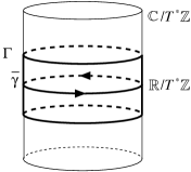
Figure 3. Riemann surface $\Gamma$. The monodromy matrix $M_{\gamma}$ is computed along the loop $\gamma$.

We return to the system (1.5) and regard $\varepsilon$ as a state variable to rewrite it as

$$\dot{I}=\varepsilon h(I,\theta;\varepsilon),\quad\dot{\theta}=\omega(I)+\varepsilon g(I,\theta;\varepsilon),\quad\dot{\varepsilon}=0,$$ (2.8)

like (2.4). We extend the domain of the independent variable $t$ to a region including $\mathbb{R}$ in $\mathbb{C}$, as stated in Theorem 2.1. The $(k+1)$th-order RVE of (2.8) along the periodic orbit $(I,\theta,\varepsilon)=(I^{\ast},\omega(I^{\ast})t+\theta_{0},0)$ is given by

$$\begin{split}&\dot{\xi}=h^{k}(I^{\ast},\omega^{\ast}t+\theta_{0};0)\lambda,\\ &\dot{\eta}=\mathrm{D}\omega(I^{\ast})\xi+g^{k}(I^{\ast},\omega^{\ast}t+\theta_{0};0)\lambda,\\ &\dot{\lambda}=0,\end{split}\quad(\xi,\eta,\chi)\in\mathbb{C}^{\ell}\times\mathbb{C}^{m}\times\mathbb{C}.$$ (2.9)

where

$$h^{k}(I,\theta)=\frac{1}{k!}\mathrm{D}_{\varepsilon}^{k}h(I,\theta;0),\quad g^{k}(I,\theta)=\frac{1}{k!}\mathrm{D}_{\varepsilon}^{k}g(I,\theta;0).$$

As a Riemann surface, we take any region $\Gamma$ in $\mathbb{C}/T^{\ast}\mathbb{Z}$ such that the closed loop $\gamma_{\theta}$ in assumption (A2) as well as $\mathbb{R}/T^{\ast}\mathbb{Z}$ is contained in $\Gamma$, as in Theorem 2.1. See Fig. 3. Let $\mathbb{K}_{\theta}\neq\mathbb{C}$ be a differential field that consists of $T^{\ast}$-periodic functions and contains the elements of $h^{k}(I^{\ast},\omega(I^{\ast})t+\theta)$ and $g^{k}(I^{\ast},\omega(I^{\ast})t+\theta)$ with $t\in\Gamma$. We regard the $(k+1)$th-order RVE (2.9) as a linear differential equation over $\mathbb{K}_{\theta}$ on the Riemann surface $\Gamma$. We obtain a fundamental matrix of (2.9) as

$$\Phi^{k}(t;\theta_{0})=\begin{pmatrix}\mathrm{id}_{\ell}&0&\Xi^{k}(t;\theta_{0})\\ \mathrm{D}\omega(I^{\ast})t&\mathrm{id}_{m}&\Psi^{k}(t;\theta_{0})\\ 0&0&1\end{pmatrix},$$

where

$$\Xi^{k}(t;\theta)= \int_{0}^{t}h^{k}(I^{\ast},\omega(I^{\ast})\tau+\theta)\mathrm{d}\tau,$$

$$\Psi^{k}(t;\theta)= \int_{0}^{t}\bigl{(}\mathrm{D}\omega(I^{\ast})\Xi(\tau;\theta)+g^{k}(I^{\ast},\omega(I^{\ast})\tau+\theta)\bigr{)}\mathrm{d}\tau.$$

Let $\mathscr{G}_{\theta}$ be the differential Galois group of (2.9) and let $\sigma\in\mathscr{G}_{\theta}$. Then

$$\frac{\mathrm{d}}{\mathrm{d}t}\sigma(\Xi^{k}(t;\theta))=\sigma\left(\frac{\mathrm{d}}{\mathrm{d}t}\Xi^{k}(t;\theta)\right)=h^{k}(I^{\ast},\omega(I^{\ast})t+\theta),$$

so that

$$\sigma(\Xi^{k}(t;\theta))=\int_{0}^{t}h^{k}(I^{\ast},\omega(I^{\ast})\tau+\theta;0)\mathrm{d}\tau+C=\Xi^{k}(t;\theta)+C,$$ (2.10)

where $C$ is a constant $\ell$-dimensional vector depending on $\sigma$. If $\Xi^{k}(t;\theta)\in\mathbb{K}_{\theta}$, then $C=0$ for any $\sigma\in\mathscr{G}_{\theta}$. Similarly, we have

$$\sigma(\mathrm{D}\omega(I^{\ast})t)=\mathrm{D}\omega(I^{\ast})t+C^{\prime},$$

where $C^{\prime}$ is a constant $m\times\ell$ matrix depending on $\sigma$. If $\mathrm{D}\omega(I^{\ast})\neq 0$, then $C^{\prime}\neq 0$ for some $\sigma\in\mathscr{G}_{\theta}$ since $\mathrm{D}\omega(I^{\ast})t\notin\mathbb{K}_{\theta}$. On the other hand,

$$\frac{\mathrm{d}}{\mathrm{d}t}\sigma(\Psi^{k}(t;\theta))= \sigma\left(\frac{\mathrm{d}}{\mathrm{d}t}\Psi^{k}(t;\theta)\right)=\sigma\bigl{(}\mathrm{D}\omega(I^{\ast})\Xi^{k}(t;\theta)+g^{k}(I^{\ast},\omega(I^{\ast})t+\theta)\bigr{)}$$

$$= \mathrm{D}\omega(I^{\ast})\Xi^{k}(t;\theta)+g^{k}(I^{\ast},\omega(I^{\ast})t+\theta)+\mathrm{D}\omega(I^{\ast})C.$$

Hence,

$$\sigma(\Psi^{k}(t;\theta))=\Psi^{k}(t;\theta)+\mathrm{D}\omega(I^{\ast})Ct+C^{\prime\prime},$$

where $C^{\prime\prime}$ is a constant $m$-dimensional vector depending on $\sigma$. If $\Xi^{k}(t;\theta),\Psi^{k}(t;\theta)\in\mathbb{K}_{\theta}$, then $C^{\prime\prime}=0$ for any $\sigma\in\mathscr{G}_{\theta}$. Thus, we see that

$$\mathscr{G}_{\theta}\subset\tilde{\mathscr{G}}:=\{M(C_{1},C_{2},C_{3})\mid C_{1}\in\mathbb{C}^{\ell},C_{2}\in\mathbb{C}^{m},C_{3}\in\mathbb{C}^{m\times\ell}\},$$

where

$$M(C_{1},C_{2},C_{3})=\begin{pmatrix}\mathrm{id}_{\ell}&0&C_{1}\\ C_{3}&\mathrm{id}_{m}&C_{2}\\ 0&0&1\end{pmatrix}.$$

Proof of Theorem 2.1.

Assume that the hypotheses of the theorem hold. We fix $\theta\in\mathbb{T}^{m}$ such that the integral (2.2) is not zero. We continue the fundamental matrix $\Phi^{k}(t;\theta)$ analytically along the loop $\gamma_{\theta}$ to obtain the monodromy matrix as

$$M_{\gamma}=\begin{pmatrix}\mathrm{id}_{\ell}&0&\hat{C}_{1}\\ 0&\mathrm{id}_{m}&\hat{C}_{2}\\ 0&0&1\end{pmatrix},$$ (2.11)

where

$$\hat{C}_{1}=\int_{\gamma_{\theta}}h^{k}(I^{\ast},\omega(I^{\ast})t+\theta;0)\mathrm{d}\tau,$$

$$\hat{C}_{2}=\int_{\gamma_{\theta}}\bigl{(}\mathrm{D}\omega(I^{\ast})\Xi^{k}(\tau;\theta)+g^{k}(I^{\ast},\omega(I^{\ast})\tau+\theta)\bigr{)}\mathrm{d}\tau.$$

See Appendix B for basic information on monodromy matrices. In particular, we have $M_{\gamma}\in\mathscr{G}_{\theta}$. Note that $\mathrm{D}\omega(I^{\ast})\hat{C}_{1}\neq 0$ by assumption (A2).

Let $\bar{\gamma}=\{T^{\ast}s\mid s\in[0,1]\}$, which is also a closed loop on the Riemann surface $\Gamma$ (see Fig. 3). We continue $\Phi^{k}(t;\theta)$ analytically along the loop $\bar{\gamma}$ to obtain the monodromy matrix as

$$M_{\bar{\gamma}}=\begin{pmatrix}\mathrm{id}_{\ell}&0&\Xi^{k}(T^{\ast};\theta)\\ \mathrm{D}\omega(I^{\ast})T^{\ast}&\mathrm{id}_{m}&\Psi^{k}(T^{\ast};\theta)\\ 0&0&1\end{pmatrix}.$$

Let $\bar{C}_{1}=\Xi^{k}(T^{\ast};\theta)$, $\bar{C}_{2}=\Psi^{k}(T^{\ast};\theta)$ and $\bar{C}_{3}=\mathrm{D}\omega(I^{\ast})T^{\ast}$. We see that $M_{\bar{\gamma}}=M(\bar{C}_{1},\bar{C}_{2},\bar{C}_{3})\in\mathscr{G}_{\theta}$ and $\bar{C}_{3}\hat{C}_{1}\neq 0$ by $\mathrm{D}\omega(I^{\ast})\hat{C}_{1}\neq 0$.

Lemma 2.5.

Suppose that $M(C_{1},C_{2},C_{3}),M(C_{1}^{\prime},C_{2}^{\prime},C_{3}^{\prime})\in\mathscr{G}_{\theta}$ for some $C_{j},C_{j}^{\prime}$, $j=1,2,3$, with $C_{3}C_{1}^{\prime}\neq C_{3}^{\prime}C_{1}$. Then the identity component $\mathscr{G}_{\theta}^{0}$ of $\mathscr{G}_{\theta}$ is not commutative.

Proof.

Assume that the hypothesis holds. We easily see that $M(C_{1},C_{2},C_{3})$ and $M(C_{1}^{\prime},C_{2}^{\prime},C_{3}^{\prime})$ is not commutative since

$$M(C_{1},C_{2},C_{3})M(C_{1}^{\prime},C_{2}^{\prime},C_{3})=\begin{pmatrix}\mathrm{id}_{\ell}&0&C_{1}+C_{1}^{\prime}\\ C_{3}+C_{3}^{\prime}&\mathrm{id}_{m}&C_{3}C_{1}^{\prime}+C_{2}+C_{2}^{\prime}\\ 0&0&1\end{pmatrix}$$

while

$$M(C_{1}^{\prime},C_{2}^{\prime},C_{3})M(C_{1}^{\prime},C_{2}^{\prime},C_{3})=\begin{pmatrix}\mathrm{id}_{\ell}&0&C_{1}+C_{1}^{\prime}\\ C_{3}+C_{3}^{\prime}&\mathrm{id}_{m}&C_{3}^{\prime}C_{1}+C_{2}+C_{2}^{\prime}\\ 0&0&1\end{pmatrix}.$$

On the other hand, we compute

$$M(C_{1},C_{2},C_{3})^{2}= \begin{pmatrix}\mathrm{id}_{\ell}&0&C_{1}\\ C_{3}&\mathrm{id}_{m}&C_{2}\\ 0&0&1\end{pmatrix}\begin{pmatrix}\mathrm{id}_{\ell}&0&C_{1}\\ C_{3}&\mathrm{id}_{m}&C_{2}\\ 0&0&1\end{pmatrix}$$

$$= \begin{pmatrix}\mathrm{id}_{\ell}&0&2C_{1}\\ 2C_{3}&\mathrm{id}_{m}&C_{3}C_{1}+2C_{2}\\ 0&0&1\end{pmatrix}$$

and easily show by induction that

$$M(C_{1},C_{2},C_{3})^{k}=\begin{pmatrix}\mathrm{id}_{\ell}&0&kC_{1}\\ kC_{3}&\mathrm{id}_{m}&(k-1)C_{3}C_{1}+kC_{2}\\ 0&0&1\end{pmatrix}$$

for any $k\in\mathbb{N}$. Since $\mathscr{G}_{\theta}^{0}$ is a subgroup of finite index in $\mathscr{G}_{\theta}$ (see Appendix A), we show that

$$\mathscr{G}_{\theta}^{0}\supset\{M(cC_{1},(c-1)C_{3}C_{1}+cC_{2},cC_{3})\mid c\in\mathbb{C}\}$$

if $C_{3}C_{1}+C_{2}\neq 0$ and

$$\mathscr{G}_{\theta}^{0}\supset\{M(cC_{1},C_{2},cC_{3})\mid c\in\mathbb{C}\}$$

if $C_{3}C_{1}+C_{2}=0$. Thus, we show that $\mathscr{G}_{\theta}^{0}$ is not commutative in both cases. ∎

By Lemma 2.5, the identity component $\mathscr{G}_{\theta}^{0}$ is not commutative. Applying Theorem 2.3, we see that the system (1.5) is meromorphically nonintegrable near the resonant periodic orbit $(I^{\ast},\omega(I^{\ast})t+\theta)$ in the meaning of Theorem 2.1. If this statement holds for $\theta$ on a dense set $\Delta\subset\mathbb{T}^{m}$, then so does it on $\mathbb{T}^{m}$. Thus, we complete the proof. ∎

Remark 2.6.

1. When the system (1.5) is Hamiltonian, it is not meromorphically Liouville-integrable such that the first integrals also depend meromorphically on $\varepsilon$ near $\varepsilon=0$, if the hypotheses of Theorem 2.1 hold.

2. We see that when the closed loop $\gamma_{\theta}$ can be taken independently of $\theta$, the integral $\mathscr{I}^{k}(\theta)$ is an analytic function of $\theta$, so that by the proof of Theorem 2.1 assumption (A2) holds if $\mathscr{I}^{k}(\theta)$ is not identically zero.

3. Assumption (A2) in Theorem 2.1 may be replaced with
   

   1. $\mathrm{D}\omega(I^{\ast})\Xi^{k}(t;\theta)\notin\mathbb{K}_{\theta}(t)$.
      

   This is easily proven as follows. Let $\mathbb{L}$ be the Picard-Vessiot extension of (2.9) and let $\hat{\sigma}:\mathbb{L}\to\mathbb{L}$ be a $\mathbb{K}_{\theta}(t)$-automorphism, i.e., $\hat{\sigma}\in\mathrm{Gal}(\mathbb{L}/\mathbb{K}_{\theta}(t))$ $($see Appendix A). Since $\hat{\sigma}\in\mathscr{G}_{\theta}$, we have

   $$\hat{\sigma}(\mathrm{D}\omega(I^{\ast})t)=\mathrm{D}\omega(I^{\ast})t,\quad\hat{\sigma}(\Xi^{k}(t;\theta))=\Xi^{k}(t;\theta)+\hat{C}_{1}$$

   as in (2.10), so that $\hat{\sigma}$ corresponds to the matrix

   $$\begin{pmatrix}\mathrm{id}_{\ell}&0&\hat{C}_{1}\\ 0&\mathrm{id}_{m}&\hat{C}_{2}\\ 0&0&1\end{pmatrix}=M(\hat{C}_{1},\hat{C}_{2},0).$$

   Since $\mathrm{D}\omega(I^{\ast})\hat{C}_{1}\neq 0$ for some $\hat{\sigma}\in\mathrm{Gal}(\mathbb{L}/\mathbb{K}_{\theta}(t))$, we only have to use the above matrix instead of (2.11) and apply the same arguments to obtain the desired result.

3. Planar Case

We prove Theorem 1.1 for the planar case (1.1). We only consider a neighborhood of $(x,y)=(-\mu,0)$ since we only have to replace $x$ and $\mu$ with $-x$ and $1-\mu$ to obtain the result for a neighborhood of $(1-\mu,0)$. We introduce a small parameter $\varepsilon$ such that $0<\varepsilon\ll 1$. Letting

$$\varepsilon^{2}\xi=x+\mu,\quad\varepsilon^{2}\eta=y,\quad\varepsilon^{-1}p_{\xi}=p_{x},\quad\varepsilon^{-1}p_{\eta}=p_{y}+\mu$$

and scaling the time variable $t\to\varepsilon^{3}t$, we rewrite (1.1) as

$$\dot{\xi}=p_{\xi}+\varepsilon^{3}\eta,\quad\dot{p}_{\xi}=-\frac{(1-\mu)\xi}{(\xi^{2}+\eta^{2})^{3/2}}+\varepsilon^{3}p_{\eta}-\varepsilon^{4}\mu-\varepsilon^{4}\frac{\mu(\varepsilon^{2}\xi-1)}{((\varepsilon^{2}\xi-1)^{2}+\varepsilon^{2}\eta^{2})^{3/2}},$$

$$\dot{\eta}=p_{\eta}-\varepsilon^{3}\xi,\quad\dot{p}_{\eta}=-\frac{(1-\mu)\eta}{(\xi^{2}+\eta^{2})^{3/2}}-\varepsilon^{3}p_{\xi}-\varepsilon^{6}\frac{\mu\eta}{((\varepsilon^{2}\xi-1)^{2}+\varepsilon^{2}\eta^{2})^{3/2}},$$

or up to the order of $\varepsilon^{6}$,

$$\begin{split}&\dot{\xi}=p_{\xi}+\varepsilon^{3}\eta,\quad\dot{p}_{\xi}=-\frac{(1-\mu)\xi}{(\xi^{2}+\eta^{2})^{3/2}}+\varepsilon^{3}p_{\eta}+2\varepsilon^{6}\mu\xi,\\ &\dot{\eta}=p_{\eta}-\varepsilon^{3}\xi,\quad\dot{p}_{\eta}=-\frac{(1-\mu)\eta}{(\xi^{2}+\eta^{2})^{3/2}}-\varepsilon^{3}p_{\xi}-\varepsilon^{6}\mu\eta,\end{split}$$ (3.1)

where the $O(\varepsilon^{8})$ terms have been eliminated. Equation (3.1) is a Hamiltonian system with the Hamiltonian

$$H=\tfrac{1}{2}(p_{\xi}^{2}+p_{\eta}^{2})-\frac{1-\mu}{\sqrt{\xi^{2}+\eta^{2}}}+\varepsilon^{3}(\eta p_{\xi}-\xi p_{\eta})-\tfrac{1}{2}\varepsilon^{6}\mu(2\xi^{2}-\eta^{2}).$$ (3.2)

Nonintegrability of a system which is similar to (3.1) but does not contain a small parameter was proven by using the Morales-Ramis theory [20, 22] in [24]. See also Remark 3.1(ii).

We next rewrite (3.2) in the polar coordinates. Let

$$\xi=r\cos\phi,\quad\eta=r\sin\phi.$$

The momenta $(p_{r},p_{\phi})$ corresponding to $(r,\phi)$ satisfy

$$p_{\xi}=p_{r}\cos\phi-\frac{p_{\phi}}{r}\sin\phi,\quad p_{\eta}=p_{r}\sin\phi+\frac{p_{\phi}}{r}\cos\phi.$$

See, e.g., Section 8.6.1 of [19]. The Hamiltonian becomes

$$H=\tfrac{1}{2}\left(p_{r}^{2}+\frac{p_{\phi}^{2}}{r^{2}}\right)-\frac{1-\mu}{r}-\varepsilon^{3}p_{\phi}-\tfrac{1}{4}\varepsilon^{6}\mu r^{2}(3\cos 2\phi+1).$$

Up to $O(1)$, the corresponding Hamiltonian system becomes

$$\dot{r}=p_{r},\quad\dot{p}_{r}=\frac{p_{\phi}^{2}}{r^{3}}-\frac{1-\mu}{r^{2}},\quad\dot{\phi}=\frac{p_{\phi}}{r^{2}},\quad\dot{p}_{\phi}=0,$$ (3.3)

which is easily solved since $p_{\phi}$ is a constant. Let $u=1/r$. From (3.3) we have

$$\frac{\mathrm{d}^{2}u}{\mathrm{d}\phi^{2}}+u=\frac{1-\mu}{p_{\phi}^{2}},$$

from which we obtain the relation

$$r=\frac{p_{\phi}^{2}}{(1-\mu)(1+e\cos\phi)},$$ (3.4)

where the position $\phi=0$ is appropriately chosen and $e$ is a constant. We choose $e\in(0,1)$, so that Eq. (3.4) represents an elliptic orbit with the eccentricity $e$. Moreover, its period is given by

$$T=\frac{p_{\phi}^{3}}{(1-\mu)^{2}}\int_{0}^{2\pi}\frac{\mathrm{d}\phi}{(1+e\cos\phi)^{2}}=\frac{2\pi p_{\phi}^{3}}{(1-\mu)^{2}(1-e^{2})^{3/2}}.$$ (3.5)

Now we introduce the Delaunay elements obtained from the generating function

$$W(r,\phi,I_{1},I_{2})=I_{2}\phi+\chi(r,I_{1},I_{2}),$$ (3.6)

where

$$\chi(r,I_{1},I_{2})= \int_{r_{-}}^{r}\left(\frac{2(1-\mu)}{\rho}-\frac{(1-\mu)}{I_{1}^{2}}-\frac{I_{2}^{2}}{\rho^{2}}\right)^{1/2}\mathrm{d}\rho$$

$$= -2I_{1}^{2}\arcsin\sqrt{\frac{r_{+}-r}{r_{+}-r_{-}}}+\sqrt{(r_{+}-r)(r-r_{-})}$$

$$+\frac{2I_{1}I_{2}}{\sqrt{1-\mu}}\arctan\sqrt{\frac{r_{-}(r_{+}-r)}{r_{+}(r-r_{-})}}$$ (3.7)

with

$$r_{\pm}=I_{1}\left(I_{1}\pm\sqrt{I_{1}^{2}-\frac{I_{2}^{2}}{1-\mu}}\right)$$

(see, e.g., Section 8.9.1 of [19]). We have

$$p_{r}=\frac{\partial W}{\partial r}=\frac{\partial\chi}{\partial r}(r,I_{1},I_{2}),\quad p_{\phi}=\frac{\partial W}{\partial\phi}=I_{2},$$

$$\theta_{1}=\frac{\partial W}{\partial I_{1}}=\chi_{1}(r,I_{1},I_{2}),\quad\theta_{2}=\frac{\partial W}{\partial I_{2}}=\phi+\chi_{2}(r,I_{1},I_{2}),$$

where

$$\chi_{1}(r,I_{1},I_{2})=\frac{\partial\chi}{\partial I_{1}}(r,I_{1},I_{2}),\quad\chi_{2}(r,I_{1},I_{2})=\frac{\partial\chi}{\partial I_{2}}(r,I_{1},I_{2}).$$

Since the transformation from $(r,\phi,p_{r},p_{\phi})$ to $(\theta_{1},\theta_{2},I_{1},I_{2})$ is symplectic, the transformed system is also Hamiltonian and its Hamiltonian is given by

$$H= -\frac{(1-\mu)}{2I_{1}^{2}}-\varepsilon^{3}I_{2}$$

$$-\tfrac{1}{4}\varepsilon^{6}\mu R(\theta_{1},I_{1},I_{2})^{2}(3\cos 2(\theta_{2}-\chi_{2}(R(\theta_{1},I_{1},I_{2}),I_{1},I_{2}))+1),$$

where $r=R(\theta_{1},I_{1},I_{2})$ is the $r$-component of the symplectic transformation satisfying

$$\theta_{1}=\chi_{1}(R(\theta_{1},I_{1},I_{2}),I_{1},I_{2}).$$ (3.8)

Thus, we obtain the Hamiltonian system

$$\begin{split}\dot{I}_{1}=&\tfrac{1}{2}\varepsilon^{6}\mu\frac{\partial R}{\partial\theta_{1}}(\theta_{1},I_{1},I_{2})R(\theta_{1},I_{1},I_{2})\biggl{(}3\cos 2(\theta_{2}-\chi_{2}(R(\theta_{1},I_{1},I_{2}),I_{1},I_{2}))\\ &\quad+1+3R(\theta_{1},I_{1},I_{2})\frac{\partial\chi_{2}}{\partial r}(R(\theta_{1},I_{1},I_{2}),I_{1},I_{2})\\ &\quad\times\sin 2(\theta_{2}-\chi_{2}(R(\theta_{1},I_{1},I_{2}),I_{1},I_{2}))\biggr{)},\\ \dot{I}_{2}=&-\tfrac{3}{2}\varepsilon^{6}\mu R(\theta_{1},I_{1},I_{2})^{2}\sin 2(\theta_{2}-\chi_{2}(R(\theta_{1},I_{1},I_{2}),I_{1},I_{2})),\\ \dot{\theta}_{1}=&\frac{1-\mu}{I_{1}^{3}}+O(\varepsilon^{6}),\quad\dot{\theta}_{2}=-\varepsilon^{3}+O(\varepsilon^{6}).\end{split}$$ (3.9)

Similarly to the treatment for (1.1) stated just above Theorem 1.1, the new variables $(v_{1},v_{2},v_{3})\in\mathbb{C}\times(\mathbb{C}/2\pi\mathbb{Z})^{2}$ given by

$$V_{1}(v_{1},r,I_{1},I_{2}):= v_{1}^{2}+r^{2}-2I_{1}^{2}r+\frac{I_{1}^{2}I_{2}^{2}}{1-\mu}=0,$$

$$V_{2}(v_{2},r,I_{1},I_{2}):= I_{1}^{2}\left(I_{1}^{2}-\frac{I_{2}^{2}}{1-\mu}\right)(2\sin^{2}v_{2}-1)^{2}-(r-I_{1}^{2})^{2}=0,$$

$$V_{3}(v_{3},r,I_{1},I_{2}):= I_{1}^{2}\left(r-\frac{I_{2}^{2}}{1-\mu}\right)^{2}(\tan^{2}v_{3}+1)^{2}$$

$$-r^{2}\left(I_{1}^{2}-\frac{I_{2}^{2}}{1-\mu}\right)^{2}(\tan^{2}v_{3}-1)^{2}=0$$

are introduced, so that the generating function (3.6) is regarded as an analytic one on the four-dimensional complex manifold

$$\bar{\mathscr{S}}_{2}=\{(r,\phi,I_{1},I_{2},v_{1},v_{2},v_{3}) \in\mathbb{C}\times(\mathbb{C}/2\pi\mathbb{Z})\times\mathbb{C}^{3}\times(\mathbb{C}/2\pi\mathbb{Z})^{2}$$

$$\mid V_{j}(v_{j},r,I_{1},I_{2})=0,\ j=1,2,3\}$$

since Eq. (3.7) is represented by

$$\chi(I_{1},I_{2},v_{1},v_{2},v_{3})=v_{1}-2I_{1}^{2}v_{2}+\frac{2I_{1}I_{2}v_{3}}{\sqrt{1-\mu}}.$$

Hence, we can regard (3.9) as a meromorphic two-degree-of-freedom Hamiltonian systems on the four-dimensional complex manifold

$$\hat{\mathscr{S}}_{2}= \{(I_{1},I_{2},\theta_{1},\theta_{2},r,v_{1},v_{2},v_{3})\in\mathbb{C}^{2}\times(\mathbb{C}/2\pi\mathbb{Z})^{2}\times\mathbb{C}^{2}\times(\mathbb{C}/2\pi\mathbb{Z})^{2}$$

$$\quad\mid\theta_{1}-\chi_{1}(r,I_{1},I_{2})=V_{j}(v_{j},r,I_{1},I_{2})=0,\ j=1,2,3\},$$

like (1.3) on $\mathscr{S}_{2}$ for (1.1). Actually, we have

$$\frac{\partial V_{j}}{\partial v_{j}}\frac{\partial v_{j}}{\partial r}+\frac{\partial V_{j}}{\partial r}=0,\quad\frac{\partial V_{j}}{\partial v_{j}}\frac{\partial v_{j}}{\partial I_{l}}+\frac{\partial V_{j}}{\partial I_{l}}=0,\quad j=1,2,3,\ l=1,2,$$

to express

$$\frac{\partial\chi}{\partial r}=\sum_{j=1}^{3}\frac{\partial\chi}{\partial v_{j}}\frac{\partial V_{j}}{\partial r},\quad\chi_{l}=\frac{\partial\chi}{\partial I_{l}}+\sum_{j=1}^{3}\frac{\partial\chi}{\partial v_{j}}\frac{\partial V_{j}}{\partial I_{l}},\quad l=1,2$$

as meromorophic functions of $(r,I_{1},I_{2},v_{1},v_{2},v_{3})$ on $\bar{\mathscr{S}}_{2}$. In particular, the Hamiltonian system has an additional first integral that is meromorphic in$(I_{1},I_{2},\theta_{1},\theta_{2},v_{1},v_{2},v_{3},\varepsilon)$ on $\hat{\mathscr{S}}_{2}\setminus\Sigma(\hat{\mathscr{S}}_{2})$ near $\varepsilon=0$ if the system (1.1) has an additional first integral that is meromorphic in $(x,y,p_{x},p_{y},u_{1},u_{2})$ on $\mathscr{S}_{2}\setminus\Sigma(\mathscr{S}_{2})$ near $(x,y)=(-\mu,0)$, and it does not if the hypotheses of Theorem 2.1 hold for (3.9) as in Theorem 2 of [10], since the corresponding Hamiltonian system has the same expression as (3.9) on $\hat{\mathscr{S}}_{2}\setminus\Sigma(\hat{\mathscr{S}}_{2})$, where $\Sigma(\hat{\mathscr{S}}_{2})$ is the critical set of $\hat{\mathscr{S}}_{2}$ on which the projection $\hat{\pi}_{2}:\hat{\mathscr{S}}_{2}\to\mathbb{C}^{2}\times(\mathbb{C}/2\pi\mathbb{Z})^{2}$ given by

$$\hat{\pi}_{2}(I_{1},I_{2},\theta_{1},\theta_{2},r,v_{1},v_{2},v_{3})=(I_{1},I_{2},\theta_{1},\theta_{2})$$

is singular.

We next estimate the $O(\varepsilon^{6})$-term in the first equation in (3.9) for the unperturbed solutions. When $\varepsilon=0$, we see that $I_{1},I_{2},\theta_{2}$ are constants and can write $\theta_{1}=\omega_{1}t+\theta_{10}$ for any solution to (3.9), where

$$\omega_{1}=\frac{1-\mu}{I_{1}^{3}}$$ (3.10)

and $\theta_{10}\in\mathbb{S}^{1}$ is a constant. Since $r=R(\omega_{1}t+\theta_{10},I_{1},I_{2})$ and

$$\phi=-\chi_{2}(R(\omega_{1}t+\theta_{10},I_{1},I_{2}),I_{1},I_{2}),$$

respectively, become the $r$- and $\phi$-components of a solution to (3.3), we have

$$\begin{split}&R(\omega_{1}t+\theta_{10},I_{1},I_{2})=\frac{I_{2}^{2}}{(1-\mu)(1+e\cos(\phi(t)+\bar{\phi}(\theta_{10})))},\\ &-\chi_{2}(R(\omega_{1}t+\theta_{10},I_{1},I_{2}),I_{1},I_{2})=\phi(t)+\bar{\phi}(\theta_{10})\end{split}$$ (3.11)

by (3.4), where $\phi(t)$ is the $\phi$-component of a solution to (3.3) and $\bar{\phi}(\theta_{10})$ is a constant depending on $\theta_{10}$. Differentiating both equations in (3.11) with respect to $t$ yields

$$\begin{split}&\omega_{1}\frac{\partial R}{\partial\theta_{1}}(\omega_{1}t+\theta_{10},I_{1},I_{2})=\frac{eI_{2}^{2}\sin(\phi(t)+\bar{\phi}(\theta_{10}))\dot{\phi}(t)}{(1-\mu)(1+e\cos(\phi(t)+\bar{\phi}(\theta_{10})))^{2}},\\ &-\omega_{1}\frac{\partial\chi_{2}}{\partial r}(R(\omega_{1}t+\theta_{10},I_{1},I_{2}),I_{1},I_{2})\frac{\partial R}{\partial\theta_{1}}(\omega_{1}t+\theta_{10},I_{1},I_{2})=\dot{\phi}(t).\end{split}$$ (3.12)

Using (3.11) and (3.12), we can obtain the necessary expression of the $O(\varepsilon^{6})$-term.

We are ready to check the hypotheses of Theorem 2.1. Assumption (A1) holds for any $I_{1}>0$. Fix the values of $I_{1},I_{2}$ at some $I_{1}^{\ast},I_{2}^{\ast}>0$, and let $\omega^{\ast}=\omega_{1}/3$. Since by the second equation of (3.11) $\phi(t)$ is $2\pi/\omega_{1}$-periodic, we have

$$\frac{2\pi I_{2}^{\ast 3}}{(1-\mu)^{2}(1-e^{2})^{3/2}}=\frac{2\pi I_{1}^{3}}{1-\mu}$$

by (3.5) and (3.10), so that

$$I_{2}^{\ast}=I_{1}^{\ast}(1-\mu)^{1/3}\sqrt{1-e^{2}}.$$

From (3.10) we also have

$$\mathrm{D}\omega(I^{\ast})= \begin{pmatrix}-3(1-\mu)/I_{1}^{\ast 4}&0\\ 0&0\end{pmatrix},$$

where $I^{\ast}=(I_{1}^{\ast},I_{2}^{\ast})$. We write the first component of (2.2) with $k=5$ for $I=I^{\ast}$ as

$$\mathscr{I}_{1}^{5}(\theta)= -\frac{3\mu(1-\mu)}{2I_{1}^{\ast 4}}\int_{\gamma_{\theta}}\biggl{(}\frac{\partial R}{\partial\theta_{1}}(\omega_{1}t+\theta_{1},I_{1}^{\ast},I_{2}^{\ast})R(\omega_{1}t+\theta_{1},I_{1}^{\ast},I_{2}^{\ast})$$

$$\times\biggl{(}3\cos 2(\theta_{2}-\chi_{2}(R(\omega_{1}t+\theta_{1},I_{1}^{\ast},I_{2}^{\ast}),I_{1}^{\ast},I_{2}^{\ast}))+1$$

$$+3R(\omega_{1}t+\theta_{1},I_{1}^{\ast},I_{2}^{\ast})\frac{\partial\chi_{2}}{\partial r}(R(\omega_{1}t+\theta_{1},I_{1}^{\ast},I_{2}^{\ast}),I_{1}^{\ast},I_{2}^{\ast})$$

$$\times\sin 2(\theta_{2}-\chi_{2}(R(\omega_{1}t+\theta_{1},I_{1}^{\ast},I_{2}^{\ast}),I_{1}^{\ast},I_{2}^{\ast}))\biggr{)}\mathrm{d}t,$$

where the closed loop $\gamma_{\theta}$ is specified below. Using (3.11) and (3.12), we compute

$$\mathscr{I}_{1}^{5}(\theta)= \frac{3\mu I_{2}^{\ast 4}}{2(1-\mu)^{2}I_{1}^{\ast}}\int_{\gamma_{\theta}}\dot{\phi}(t)\biggl{(}\frac{3\sin 2(\phi(t)+\bar{\phi}(\theta_{1})+\theta_{2})}{(1+e\cos(\phi(t)+\bar{\phi}(\theta_{1})))^{2}}$$

$$-\frac{e\sin(\phi(t)+\bar{\phi}(\theta_{1}))(3\cos 2(\phi(t)+\bar{\phi}(\theta_{1})+\theta_{2})+1)}{(1+e\cos(\phi(t)+\bar{\phi}(\theta_{1})))^{3}}\biggr{)}\mathrm{d}t.$$ (3.13)

By (3.3) and (3.4) we have

$$\frac{\dot{\phi}(t)}{(1+e\cos\phi(t))^{2}}=\frac{(1-\mu)^{2}}{I_{2}^{\ast 3}}=\frac{\omega_{1}}{(1-e^{2})^{3/2}}.$$ (3.14)

Using integration by substitution and the relation (3.14), we rewrite the above integral as

$$\mathscr{I}_{1}^{5}(\theta)= \frac{9\mu I_{2}^{\ast}}{2I_{1}^{\ast}}\int_{\gamma_{\theta}}\biggl{(}\sin 2(\phi(t)+\theta_{2})-\frac{e\sin\phi(t)(\cos 2(\phi(t)+\theta_{2})+\tfrac{1}{3})}{1+e\cos\phi(t)}\biggr{)}\mathrm{d}t,$$ (3.15)

where the path of integration might change but the same notation $\gamma_{\theta}$ has still been used for it.

Figure 4. Dependence of $K_{1}$ on $e$.

On the other hand, we integrate (3.14) to obtain

$$\omega_{1}t=2\arctan\biggl{(}\frac{(1-e)\tan\tfrac{1}{2}\phi}{\sqrt{1-e^{2}}}\biggr{)}-\frac{e\sqrt{1-e^{2}}\sin\phi}{1+e\cos\phi}\quad\mbox{for $\phi\in(-\pi,\pi)$},$$ (3.16)

which is rewritten as

$$\omega_{1}t=2\operatorname{arccot}\biggl{(}\frac{(1-e)\cot(\tfrac{1}{2}(\phi+\pi)}{\sqrt{1-e^{2}}}\biggr{)}-\frac{e\sqrt{1-e^{2}}\sin\phi}{1+e\cos\phi}+\pi\quad\mbox{for $\phi\in(0,2\pi)$},$$ (3.17)

when $\phi(0)=0$ or $\lim_{t\to 0}\phi(t)=0$. From (3.16) we see that as $\operatorname{Im}\phi\to\infty$, $\omega_{1}t\to iK_{1}$, where

$$K_{1}=2\operatorname{arctanh}\biggl{(}\frac{1-e}{\sqrt{1-e^{2}}}\biggr{)}-\sqrt{1-e^{2}}>0.$$

See Fig. 4. So the integrand in (3.15) is singular at $t=iK_{1}$. Let $K_{2}=\operatorname{arccosh}(1/e)$. Then $1+e\cos\phi=0$ at $\phi=\pi+iK_{2}$, and by (3.17)

$$\frac{1}{\omega_{1}t}=\frac{1}{\sqrt{1-e^{2}}}\Delta\phi+o(\Delta\phi)$$

near $\phi=\pi+iK_{2}$, where $\Delta\phi=\phi-(\pi+iK_{2})$. Moreover, near $\phi=\pi+iK_{2}$,

$$\sin\phi=-\frac{i\sqrt{1-e^{2}}}{e}+O(\Delta\phi),\quad\cos\phi=-\frac{1}{e}+\frac{i\sqrt{1-e^{2}}}{e}\Delta\phi+O(\Delta\phi^{2}),$$

$$\sin 2\phi=\frac{2i\sqrt{1-e^{2}}}{e^{2}}+O(\Delta\phi),\quad\cos 2\phi=\frac{2-e^{2}}{e^{2}}+O(\Delta\phi).$$

Figure 5. Closed path $\gamma_{\theta}$.

We take a closed path starting and ending at $t=\tfrac{1}{3}T^{\ast}$ and passing through $t=\tfrac{2}{3}T^{\ast}$, $\tfrac{2}{3}T^{\ast}+i(K_{1}\mp\delta)$, $\tfrac{2}{3}T^{\ast}+iM$, $\tfrac{1}{3}T^{\ast}+iM$ and $\tfrac{1}{3}T^{\ast}+i(K_{1}\pm\delta)$ as $\gamma_{\theta}$ in $\mathbb{C}/T^{\ast}\mathbb{Z}$, where $\delta$ and $M$ are, respectively, sufficiently small and large positive constants. See Fig. 5. Here $\gamma_{\theta}$ passes along the left circular arc centered at $\tfrac{2}{3}T^{\ast}+iK_{1}$ (resp. at $\tfrac{1}{3}T^{\ast}+iK_{1}$) with radius $\delta$ between $\tfrac{2}{3}T^{\ast}+i(K_{1}-\delta)$ and $\tfrac{2}{3}T^{\ast}+i(K_{1}+\delta)$ (resp. between $\tfrac{1}{3}T^{\ast}+i(K_{1}+\delta)$ and $\tfrac{1}{3}T^{\ast}+i(K_{1}-\delta)$). We compute

$$\int_{2T^{\ast}\!/3+iM}^{T^{\ast}\!/3+iM}\frac{\sin\phi(t)(\cos 2(\phi(t)+\theta_{2})+\tfrac{1}{3})}{1+e\cos\phi(t)}\mathrm{d}t$$

$$=-\int_{2T^{\ast}\!/3}^{T^{\ast}\!/3}\biggl{(}\frac{2-e^{2}}{e^{3}\sqrt{1-e^{2}}}\cos 2\theta_{2}-\frac{2i}{e^{3}}\sin 2\theta_{2}+\frac{1}{3e\sqrt{1-e^{2}}}\biggr{)}i\omega_{1}M\,\mathrm{d}t+O(1)$$

$$=\frac{2\pi}{e^{3}}\biggl{(}\frac{2-e^{2}}{\sqrt{1-e^{2}}}i\cos 2\theta_{2}+2\sin 2\theta_{2}+\frac{ie^{2}}{3\sqrt{1-e^{2}}}\biggr{)}+O(1),$$

while

$$\int_{2T^{\ast}\!/3+iM}^{T^{\ast}\!/3+iM}\sin 2(\phi(t)+\theta_{2})\mathrm{d}t=O(1).$$

Moreover, the integral on $[\tfrac{1}{3}T^{\ast},\tfrac{2}{3}T^{\ast}]$ in (3.15) is $O(1)$, and the integrals from $\tfrac{2}{3}T^{\ast}$ to $\tfrac{2}{3}T^{\ast}+iM$ and from $\tfrac{1}{3}T^{\ast}+iM$ to $\tfrac{1}{3}T^{\ast}$ cancel since the integrand is $\tfrac{1}{3}T^{\ast}$-periodic.. Thus, we see that the integral (3.15) is not zero for $M>0$ sufficiently large, so that assumption (A2) holds.

Finally, we apply Theorem 2.1 to show that the meromorphic Hamiltonian system corresponding to (3.9) is not meromorphically integrable such that the first integral depends meromorphically on $\varepsilon$ near $\varepsilon=0$ even if any higher-order terms are included. Thus, we obtain the conclusion of Theorem 1.1 for the planar case. ∎

Remark 3.1.

1. The reader may think that a small circle centered at $t=\tfrac{1}{3}T^{\ast}+iK_{1}$ or $\tfrac{2}{3}T^{\ast}+iK_{1}$ can be taken as $\gamma_{\theta}$ in the proof, since the integrand in (3.15) is singular there. However, the integral (3.15) for the path is estimated to be zero $($cf. Section $3$ of [41]$)$.

2. The different change of coordinates

   $$\varepsilon\xi=x+\mu,\quad\varepsilon\eta=y,\quad p_{\xi}=p_{x},\quad p_{\eta}=p_{y}+\mu$$

   in (1.1) yields

   $$\begin{split}&\dot{\xi}=p_{\xi}+\varepsilon\eta,\quad\dot{p}_{\xi}=\varepsilon p_{\eta}-\varepsilon^{-1}\frac{(1-\mu)\xi}{(\xi^{2}+\eta^{2})^{3/2}}+2\varepsilon^{2}\mu\xi,\\ &\dot{\eta}=p_{\eta}-\varepsilon\xi,\quad\dot{p}_{\eta}=-\varepsilon p_{\xi}-\varepsilon^{-1}\frac{(1-\mu)\eta}{(\xi^{2}+\eta^{2})^{3/2}}-\varepsilon^{2}\mu\eta\end{split}$$ (3.18)

   up to $O(\varepsilon^{2})$ after the time scaling $t\to t/\varepsilon$. As in [24] we use the Levi-Civita regularization

   $$\begin{pmatrix}\xi\\ \eta\end{pmatrix}=\begin{pmatrix}q_{1}&-q_{2}\\ q_{2}&q_{1}\end{pmatrix}\begin{pmatrix}q_{1}\\ q_{2}\end{pmatrix},\quad\begin{pmatrix}p_{\xi}\\ p_{\eta}\end{pmatrix}=\frac{2}{q_{1}^{2}+q_{2}^{2}}\begin{pmatrix}q_{1}&-q_{2}\\ q_{2}&q_{1}\end{pmatrix}\begin{pmatrix}p_{1}\\ p_{2}\end{pmatrix},$$

   $($see, e.g.,[31] or Section $8.8.1$ of [19]$)$ to obtain

   $$H+C_{0}= \frac{4}{q_{1}^{2}+q_{2}^{2}}\bigl{(}\tfrac{1}{4}C_{0}(q_{1}^{2}+q_{2}^{2})+\tfrac{1}{2}(p_{1}^{2}+p_{2}^{2})+\tfrac{1}{2}\varepsilon(q_{1}^{2}+q_{2}^{2})(q_{2}p_{1}-q_{1}p_{2})$$

   $$-\tfrac{1}{2}\varepsilon^{2}\mu(q_{1}^{2}+q_{2}^{2})(q_{1}^{4}q_{1}^{2}q_{2}^{2}-4+q_{2}^{4}))-\tfrac{1}{4}\varepsilon^{-1}(1-\mu)\bigr{)},$$

   which yields

   $$H+C_{0}= \frac{4}{q_{1}^{2}+q_{2}^{2}}\bigl{(}\tfrac{1}{4}C_{0}(q_{1}^{2}+q_{2}^{2})+\tfrac{1}{2}(p_{1}^{2}+p_{2}^{2})+\tfrac{1}{2}(q_{1}^{2}+q_{2}^{2})(q_{2}p_{1}-q_{1}p_{2})$$

   $$-\tfrac{1}{2}\mu(q_{1}^{2}+q_{2}^{2})(q_{1}^{4}q_{1}^{2}q_{2}^{2}-4+q_{2}^{4}))-\tfrac{1}{4}(1-\mu)\bigr{)}$$

   after the scaling $(q,p)\to(q,p)/\varepsilon^{3/2}$. Using the approach of [24], we can show that the Hamiltonian system with the Hamiltonian

   $$\tilde{H}= \tfrac{1}{4}C_{0}(q_{1}^{2}+q_{2}^{2})+\tfrac{1}{2}(p_{1}^{2}+p_{2}^{2})+\tfrac{1}{2}(q_{1}^{2}+q_{2}^{2})(q_{2}p_{1}-q_{1}p_{2})$$

   $$-\tfrac{1}{2}\mu(q_{1}^{2}+q_{2}^{2})(q_{1}^{4}q_{1}^{2}q_{2}^{2}-4+q_{2}^{4})$$

   is meromorphically nonintegrable. This implies that the Hamiltonian (3.18) is also meromorphically nonintegrable for $\varepsilon>0$ fixed.

4. Spatial Case

We prove Theorem 1.1 for the spatial case (1.2). As in the planar case, we only consider a neighborhood of $(x,y,z)=(-\mu,0,0)$ and introduce a small parameter $\varepsilon$ such that $0<\varepsilon\ll 1$. Letting

$$\varepsilon^{2}\xi=x+\mu,\quad\varepsilon^{2}\eta=y,\quad\varepsilon^{2}\zeta=z,$$

$$\varepsilon^{-1}p_{\xi}=p_{x},\quad\varepsilon^{-1}p_{\eta}=p_{y}+\mu,\quad\varepsilon^{-1}p_{\zeta}=p_{z}$$

and scaling the time variable $t\to\varepsilon^{3}t$, we rewrite (1.2) as

$$\dot{\xi}=p_{\xi}+\varepsilon^{3}\eta,\quad\dot{\eta}=p_{\eta}-\varepsilon^{3}\xi,\quad\dot{\zeta}=p_{\zeta},$$

$$\dot{p}_{\xi}=-\frac{(1-\mu)\xi}{(\xi^{2}+\eta^{2}+\zeta^{2})^{3/2}}+\varepsilon^{3}p_{\eta}-\varepsilon^{4}\mu-\varepsilon^{4}\frac{\mu(\varepsilon\xi-1)}{((\varepsilon\xi-1)^{2}+\varepsilon^{2}(\eta^{2}+\zeta^{2}))^{3/2}},$$

$$\dot{p}_{\eta}=-\frac{(1-\mu)\eta}{(\xi^{2}+\eta^{2}+\zeta^{2})^{3/2}}-\varepsilon^{3}p_{\xi}-\varepsilon^{6}\frac{\mu\eta}{((\varepsilon\xi-1)^{2}+\varepsilon^{2}(\eta^{2}+\zeta^{2}))^{3/2}},$$

$$\dot{p}_{\zeta}=-\frac{(1-\mu)\zeta}{(\xi^{2}+\eta^{2}+\zeta^{2})^{3/2}}-\varepsilon^{6}\frac{\mu\zeta}{((\varepsilon\xi-1)^{2}+\varepsilon^{2}(\eta^{2}+\zeta^{2})))^{3/2}},$$

or up to the order of $\varepsilon^{6}$,

$$\begin{split}&\dot{\xi}=p_{\xi}+\varepsilon^{3}\eta,\quad\dot{p}_{\xi}=-\frac{(1-\mu)\xi}{(\xi^{2}+\eta^{2}+\zeta^{2})^{3/2}}+\varepsilon^{3}p_{\eta}+2\varepsilon^{6}\mu\xi,\\ &\dot{\eta}=p_{\eta}-\varepsilon^{3}\xi,\quad\dot{p}_{\eta}=-\frac{(1-\mu)\eta}{(\xi^{2}+\eta^{2}+\zeta^{2})^{3/2}}-\varepsilon^{3}p_{\xi}-\varepsilon^{6}\mu\eta,\\ &\dot{\zeta}=p_{\zeta},\quad\dot{p}_{\eta}=-\frac{(1-\mu)\zeta}{(\xi^{2}+\eta^{2}+\zeta^{2})^{3/2}},\end{split}$$ (4.1)

like (3.1), where the $O(\varepsilon^{8})$ terms have been eliminated. Equation (4.1) is a Hamiltonian system with the Hamiltonian

$$H=\tfrac{1}{2}(p_{\xi}^{2}+p_{\eta}^{2}+p_{\zeta}^{2})-\frac{1-\mu}{\sqrt{\xi^{2}+\eta^{2}+\zeta^{2}}}+\varepsilon^{3}(\eta p_{\xi}-\xi p_{\eta})-\frac{1}{2}\varepsilon^{6}(2\xi^{2}-\eta^{2}).$$ (4.2)

Figure 6. Spherical coordinates.

We next rewrite (4.2) in the spherical coordinates. See Fig. 6. Let

$$\xi=r\sin\psi\cos\phi,\quad\eta=r\sin\psi\sin\phi,\quad\zeta=r\cos\psi.$$

The momenta $(p_{r},p_{\phi},p_{\psi})$ corresponding to $(r,\phi,\psi)$ satisfy

$$p_{\xi}=p_{r}\cos\phi\sin\psi-\frac{p_{\phi}\sin\phi}{r\sin\psi}+\frac{p_{\psi}}{r}\cos\phi\cos\psi,$$

$$p_{\eta}=p_{r}\sin\phi\sin\psi+\frac{p_{\phi}\cos\phi}{r\sin\psi}+\frac{p_{\psi}}{r}\sin\phi\cos\psi,$$

$$p_{\zeta}=p_{r}\cos\psi-\frac{p_{\psi}}{r}\sin\psi$$

(see, e.g., Section 8.7 of [19]). The Hamiltonian becomes

$$H=\tfrac{1}{2}\left(p_{r}^{2}+\frac{p_{\psi}^{2}}{r^{2}}+\frac{p_{\phi}^{2}}{r^{2}\sin^{2}\psi}\right)-\frac{1-\mu}{r}-\varepsilon^{3}p_{\phi}-\frac{1}{4}\varepsilon^{6}\mu r\sin^{2}\psi(3\cos 2\phi+1).$$

Up to $O(1)$, the corresponding Hamiltonian system becomes

$$\begin{split}&\dot{r}=p_{r},\quad\dot{p}_{r}=\frac{p_{\psi}^{2}}{r^{3}}+\frac{p_{\phi}^{2}}{r^{3}\sin^{2}\psi}-\frac{1-\mu}{r^{2}},\\ &\dot{\phi}=\frac{p_{\phi}}{r^{2}\sin^{2}\psi},\quad\dot{p}_{\phi}=0,\quad\dot{\psi}=\frac{p_{\psi}}{r^{2}},\quad\dot{p}_{\psi}=\frac{p_{\phi}^{2}\cos\psi}{r^{2}\sin^{3}\psi}.\end{split}$$ (4.3)

We have the relation (3.4) for periodic orbits on the $(\xi,\eta)$-plane since Eq. (4.3) reduces to (3.3) there when $\psi=\tfrac{1}{2}\pi$ and $p_{\psi}=0$.

As in the planar case, we introduce the Delaunay elements obtained from the generating function

$$\hat{W}(r,\phi,\psi,I_{1},I_{2}.I_{2})=I_{3}\phi+\chi(r,I_{1},I_{2})+\hat{\chi}(\psi,I_{2},I_{3}),$$ (4.4)

where

$$\hat{\chi}(\psi,I_{2},I_{3})= \int_{\psi_{0}}^{\psi}\left(I_{2}^{2}-\frac{I_{3}^{2}}{\sin^{2}s}\right)^{1/2}\mathrm{d}s$$

$$= I_{2}\arctan\frac{\sqrt{I_{2}^{2}\sin^{2}\psi-I_{3}^{2}}}{I_{2}\cos\psi}-I_{3}\arctan\frac{\sqrt{I_{2}^{2}\sin^{2}\psi-I_{3}^{2}}}{I_{3}\cos\psi}$$ (4.5)

with $\psi_{0}=\arcsin(I_{3}/I_{2})$. See, e.g., Section 8.9.3 of [19], although a slightly modified generating function is used here. We have

$$\begin{split}&p_{r}=\frac{\partial\hat{W}}{\partial r}=\frac{\partial\chi}{\partial r}(r,I_{1},I_{2}),\quad p_{\phi}=\frac{\partial\hat{W}}{\partial\phi}=I_{3},\\ &p_{\psi}=\frac{\partial\hat{W}}{\partial\psi}=\frac{\partial\hat{\chi}}{\partial\psi}(\psi,I_{2},I_{3}),\quad\theta_{1}=\frac{\partial\hat{W}}{\partial I_{1}}=\chi_{1}(r,I_{1},I_{2}),\\ &\theta_{2}=\frac{\partial\hat{W}}{\partial I_{2}}=\chi_{2}(r,I_{1},I_{2})+\hat{\chi}_{2}(\psi,I_{2},I_{3}),\quad\theta_{3}=\frac{\partial\hat{W}}{\partial I_{3}}=\phi+\hat{\chi}_{3}(\psi,I_{2},I_{3}),\end{split}$$ (4.6)

where

$$\hat{\chi}_{2}(\psi,I_{2},I_{3})=\frac{\partial\hat{\chi}}{\partial I_{2}}(\psi,I_{2},I_{3}),\quad\hat{\chi}_{3}(\psi,I_{2},I_{3})=\frac{\partial\hat{\chi}}{\partial I_{3}}(\psi,I_{2},I_{3}).$$

Since the transformation from $(r,\phi,\psi,p_{r},p_{\phi},p_{\psi})$ to $(\theta_{1},\theta_{2},\theta_{3},I_{1},I_{2},I_{3})$ is symplectic, the transformed system is also Hamiltonian and its Hamiltonian is given by

$$H= -\frac{(1-\mu)}{2I_{1}^{2}}-\varepsilon^{3}I_{3}-\tfrac{1}{4}\varepsilon^{6}\mu R(\theta_{1},I_{1},I_{2})^{2}\sin^{2}\Psi(\theta_{1},\theta_{2},I_{1},I_{2},I_{3})$$

$$\quad\times(3\cos 2(\theta_{3}-\hat{\chi}_{3}(\Psi(\theta_{1},\theta_{2},I_{1},I_{2},I_{3}),I_{1},I_{2}))+1),$$

where $r=R(\theta_{1},I_{1},I_{2})$ and $\psi=\Psi(\theta_{1},\theta_{2},I_{1},I_{2},I_{3})$ are the $r$- and $\psi$-components of the symplectic transformation satisfying (3.8) and

$$\hat{\chi}_{2}(\Psi(\theta_{1},\theta_{2},I_{1},I_{2},I_{3}),I_{2},I_{3})+\chi_{2}(R(\theta_{1},I_{1},I_{2}),I_{1},I_{2})=\theta_{2},$$

respectively. Thus, we obtain the Hamiltonian system as

$$\begin{split}\dot{I}_{1}=&\tfrac{1}{2}\varepsilon^{6}\mu\hat{h}_{1}(I,\theta),\quad\dot{I}_{2}=O(\varepsilon^{6}),\quad\dot{I}_{3}=O(\varepsilon^{6}),\\ \dot{\theta}_{1}=&\frac{1-\mu}{I_{1}^{3}}+O(\varepsilon^{6}),\quad\dot{\theta}_{2}=O(\varepsilon^{6}),\quad\dot{\theta}_{3}=-\varepsilon^{3}+O(\varepsilon^{6}),\end{split}$$ (4.7)

where

$$\hat{h}_{1}(I,\theta)= \frac{\partial R}{\partial\theta_{1}}(\theta_{1},I_{1},I_{2})R(\theta_{1},I_{1},I_{2})\sin^{2}\Psi(\theta_{1},\theta_{2},I_{1},I_{2},I_{3})$$

$$\quad\times(3\cos 2(\theta_{3}-\hat{\chi}_{3}(\Psi(\theta_{1},\theta_{2},I_{1},I_{2},I_{3}),I_{2},I_{3}))+1)$$

$$+R(\theta_{1},I_{1},I_{2})^{2}\frac{\partial\Psi}{\partial\theta_{1}}(\theta_{1},\theta_{2},I_{1},I_{2},I_{3})$$

$$\quad\times\sin\Psi(\theta_{1},\theta_{2},I_{1},I_{2},I_{3})\cos\Psi(\theta_{1},\theta_{2},I_{1},I_{2},I_{3})$$

$$\quad\times(3\cos 2(\theta_{3}-\hat{\chi}_{3}(\Psi(\theta_{1},\theta_{2},I_{1},I_{2},I_{3}),I_{2},I_{3}))+1)$$

$$+3R(\theta_{1},I_{1},I_{2})^{2}\sin^{2}\Psi(\theta_{1},\theta_{2},I_{1},I_{2},I_{3})$$

$$\quad\times\frac{\partial\Psi}{\partial\theta_{1}}(\theta_{1},\theta_{2},I_{1},I_{2},I_{3})\frac{\partial\hat{\chi}_{3}}{\partial\psi}(\Psi(\theta_{1},\theta_{2},I_{1},I_{2},I_{3}),I_{2},I_{3})$$

$$\quad\times\sin 2(\theta_{3}-\hat{\chi}_{3}(\Psi(\theta_{1},\theta_{2},I_{1},I_{2},I_{3}),I_{2},I_{3})).$$

As in the planar case, the new variables $w_{1},w_{2}\in(\mathbb{C}/2\pi)$ given by

$$W_{1}(w_{1},\psi,I_{2},I_{3}):=I_{2}^{2}\cos^{2}\psi\tan^{2}w_{1}-I_{2}^{2}\sin^{2}\psi+I_{3}^{2}=0,$$

$$W_{2}(w_{2},\psi,I_{2},I_{3}):=I_{3}^{2}\cos^{2}\psi\tan^{2}w_{2}-I_{2}^{2}\sin^{2}\psi+I_{3}^{2}=0$$

are introduced, so that the generating function (4.4) is regarded as an analytic one on the six–dimensional complex manifold

$$\bar{\mathscr{S}}_{3}= \{(r,\phi,\psi,I_{1},I_{2},I_{3},v_{1},v_{2},v_{3},w_{1},w_{2})\in\mathbb{C}\times(\mathbb{C}/2\pi\mathbb{Z})^{2}\times\mathbb{C}^{4}\times(\mathbb{C}/2\pi\mathbb{Z})^{4}$$

$$\quad\mid V_{j}(v_{j},r,I_{1},I_{2})=W_{l}(w_{l},\psi,I_{2},I_{3})=0,\ j=1,2,3,\ l=1,2\}$$

since Eq. (4.5) is represented by

$$\hat{\chi}(I_{2},I_{3};v_{1},v_{2})=I_{2}w_{1}-I_{3}w_{2}.$$

Moreover, we can regard (4.7) as a meromorphic three-degree-of-freedom Hamiltonian systems on the six-dimensional complex manifold

$$\hat{\mathscr{S}}_{3}= \{(I_{1},I_{2},I_{3},\theta_{1},\theta_{2},\theta_{3},r,v_{1},v_{2},v_{3},w_{1},w_{2})\in\mathbb{C}^{3}\times(\mathbb{C}/2\pi\mathbb{Z})^{3}\times\mathbb{C}^{2}\times(\mathbb{C}/2\pi\mathbb{Z})^{4}$$

$$\quad\mid\theta_{1}-\chi_{1}(r,I_{1},I_{2})=V_{j}(v_{j},r,I_{1},I_{2})=W_{l}(w_{l},\psi,I_{2},I_{3})=0,$$

$$\qquad j=1,2,3,\ l=1,2\},$$

like (1.4) on $\mathscr{S}_{3}$ for (1.2). Actually, we have

$$\frac{\partial W_{j}}{\partial w_{j}}\frac{\partial w_{j}}{\partial\psi}+\frac{\partial W_{j}}{\partial\psi}=0,\quad\frac{\partial W_{j}}{\partial w_{j}}\frac{\partial w_{j}}{\partial I_{l}}+\frac{\partial W_{j}}{\partial I_{l}}=0,\quad j=1,2,\ l=2,3$$

to express

$$\frac{\partial\hat{\chi}}{\partial\psi}=\sum_{j=1}^{2}\frac{\partial\hat{\chi}}{\partial w_{j}}\frac{\partial W_{j}}{\partial\psi},\quad\hat{\chi}_{l}=\frac{\partial\hat{\chi}}{\partial I_{l}}+\sum_{j=1}^{2}\frac{\partial\hat{\chi}}{\partial w_{j}}\frac{\partial W_{j}}{\partial I_{l}},\quad l=2,3$$

as meromorophic functions of $(\psi,I_{2},I_{3},w_{1},w_{2})$ on $\bar{\mathscr{S}}_{3}$. In particular, the Hamiltonian system has two additional meromorphic integrals that are meromorphic in $(I_{1},I_{2},I_{3},\theta_{1},\theta_{2},\theta_{3},r,v_{1},v_{2},v_{3},w_{1},w_{2},\varepsilon)$ on $\hat{\mathscr{S}}_{3}\setminus\Sigma(\hat{\mathscr{S}}_{3})$ near $\varepsilon=0$, if the system (1.2) has two additional meromorphic integrals that are meromorphic in$(x,y,z,p_{x},p_{y},p_{z},u_{1},u_{2})$ on $\mathscr{S}_{3}\setminus\Sigma(\mathscr{S}_{3})$ near $(x,y,z)=(-\mu,0,0)$, and it does not if the hypotheses of Theorem 2.1 hold, as in the planar case. Here $\Sigma(\hat{\mathscr{S}}_{3})$ is the critical set of $\hat{\mathscr{S}}_{3}$ on which the projection $\hat{\pi}_{3}:\hat{\mathscr{S}}_{3}\to\mathbb{C}^{3}\times(\mathbb{C}/2\pi\mathbb{Z})^{3}$ given by

$$\hat{\pi}_{3}(I_{1},I_{2},I_{3},\theta_{1},\theta_{2},\theta_{3},r,v_{1},v_{2},v_{3},w_{1},w_{2})=(I_{1},I_{2},I_{3},\theta_{1},\theta_{2},\theta_{3})$$

is singular.

We next estimate the function $\hat{h}_{1}(I,\theta)$ for solutions to (4.7) with $\varepsilon=0$ on the plane of $\psi=\tfrac{1}{2}\pi$. When $\varepsilon=0$, we see that $I_{1},I_{2},I_{3},\theta_{2},\theta_{3}$ are constants and can write $\theta_{1}=\omega_{1}t+\theta_{10}$ for any solution to (4.7) with (3.10), where $\theta_{10}\in\mathbb{S}^{1}$ is a constant. Note that if $\psi=\tfrac{1}{2}\pi$ and $p_{\psi}=0$, then $I_{2}=I_{3}$ by (4.6). Since $r=R(\omega_{1}t+\theta_{10},I_{1},I_{2})$ and

$$\phi=-\hat{\chi}_{3}(\Psi(\omega_{1}t+\theta_{10},\theta_{2},I_{1},I_{3},I_{3}),I_{3},I_{3}),\quad\Psi(\omega_{1}t+\theta_{10},\theta_{2},I_{1},I_{3},I_{3})=\tfrac{1}{2}\pi,$$

respectively, become the $r$- and $\phi$-components of a solution to (4.3) with $\psi=\tfrac{1}{2}\pi$ and $p_{\psi}=0$, we have the first equation of (3.11) with

$$-\hat{\chi}_{3}(\Psi(\omega_{1}t+\theta_{10},\theta_{2},I_{1},I_{3},I_{3}),I_{3},I_{3})=\phi(t)+\bar{\phi}(\theta_{10}),$$ (4.8)

where $\phi(t)$ is the $\phi$-component of a solution to (3.3) and $\bar{\phi}(\theta_{1})$ is a constant depending only on $\theta_{1}$ as in the planar case. Differentiating (4.8) with respect to $t$ yields

$$-\omega_{1}\frac{\partial\hat{\chi}_{3}}{\partial\psi}(\Psi(\omega_{1}t+\theta_{10},\theta_{2},I_{1},I_{3},I_{3}),I_{3},I_{3})$$

$$\qquad\times\frac{\partial\Psi}{\partial\theta_{1}}(\omega_{1}t+\theta_{10},\theta_{2},I_{1},I_{3},I_{3})=\dot{\phi}(t).$$ (4.9)

Using (3.11), (3.12), (4.8) and (4.9), we can obtain the necessary expression of $\hat{h}_{1}(I,\theta)$.

We are ready to check the hypotheses of Theorem 2.1. Assumption (A1) holds for any $I_{1}>0$. Fix the value of $I_{1}$ at some $I_{1}^{\ast}>0$, and let $\omega^{\ast}=\omega_{1}/3$. By the first equation of (4.8) $\phi(t)$ is $2\pi/\omega_{1}$-periodic, so that by (3.5) and (3.10)

$$I_{2}=I_{3}=I_{1}^{\ast}(1-\mu)^{1/3}\sqrt{1-e^{2}}\ (=I_{2}^{\ast}).$$

From (3.10) we have

$$\mathrm{D}\omega(I^{\ast})=\begin{pmatrix}-3(1-\mu)/I_{1}^{\ast 4}&0&0\\ 0&0&0\\ 0&0&0\end{pmatrix},$$

where $I^{\ast}=(I_{1}^{\ast},I_{2}^{\ast},I_{2}^{\ast})$. Using the first equations of (3.11) and (3.12), (4.8) and (4.9), we compute the first component of (2.2) with $k=5$ for $I=I^{\ast}$ as

$$\mathscr{I}_{1}^{5}(\theta)= -\frac{3(1-\mu)}{I_{1}^{\ast 4}}\int_{\gamma_{\theta}}h_{1}(I^{\ast},\omega^{\ast}t+\theta_{1},\theta_{2},\theta_{3})\mathrm{d}\omega^{\ast}t$$

$$= \frac{3\mu I_{2}^{\ast 4}}{2(1-\mu)^{2}I_{1}^{\ast}}\int_{\gamma_{\theta}}\dot{\phi}(t)\biggl{(}\frac{3\sin 2(\phi(t)+\bar{\phi}(\theta_{1})+\theta_{3})}{(1+e\cos(\phi(t)+\bar{\phi}(\theta_{1})))^{2}}$$

$$+\frac{e\sin(\phi(t)+\bar{\phi}(\theta_{1}))(3\cos 2(\phi(t)+\bar{\phi}(\theta_{1})+\theta_{3})+1)}{(1+e\cos(\phi(t)+\bar{\phi}(\theta_{1})))^{3}}\biggr{)}\mathrm{d}t,$$

which has the same expression as (3.13) with $\theta_{2}=\theta_{3}$. Repeating the arguments given in Section 3, we can show that assumption (A2) holds as in the planar case. Finally, we apply Theorem 2.1 to show that the meromorphic Hamiltonian system corresponding to (4.7) is not meromorphically integrable such that the first integrals depend meromorphically on $\varepsilon$ near $\varepsilon=0$. Thus, we complete the proof of Theorem 1.1 for the spatial case. ∎

Appendix A Differential Galois Theory

In this appendix, we give necessary information on differential Galois theory for linear differential equations, which is often referred to as the Picard-Vessiot theory. See the textbooks [11, 30] for more details on the theory.

Consider a linear system of differential equations

$$y^{\prime}=Ay,\quad A\in\mathrm{gl}(n,\mathbb{K}),$$ (A.1)

where $\mathbb{K}$ is a differential field and $\mathrm{gl}(n,\mathbb{K})$ denotes the ring of $n\times n$ matrices with entries in $\mathbb{K}$. Here a differential field is a field endowed with a derivation $\partial$, which is an additive endomorphism satisfying the Leibniz rule. The set $\mathrm{C}_{\mathbb{K}}$ of elements of $\mathbb{K}$ for which $\partial$ vanishes is a subfield of $\mathbb{K}$ and called the field of constants of $\mathbb{K}$. In our application of the theory in this paper, the differential field $\mathbb{K}$ is the field of meromorphic functions on a Riemann surface, so that the field of constants is $\mathbb{C}$.

A differential field extension $\mathbb{L}\supset\mathbb{K}$ is a field extension such that $\mathbb{L}$ is also a differential field and the derivations on $\mathbb{L}$ and $\mathbb{K}$ coincide on $\mathbb{K}$. A differential field extension $\mathbb{L}\supset\mathbb{K}$ satisfying the following two conditions is called a Picard-Vessiot extension for (A.1):

1. The field $\mathbb{L}$ is generated by $\mathbb{K}$ and elements of a fundamental matrix of (A.1) ;

2. The fields of constants for $\mathbb{L}$ and $\mathbb{K}$ coincide.

The system (A.1) admits a Picard-Vessiot extension which is unique up to isomorphism.

We now fix a Picard-Vessiot extension $\mathbb{L}\supset\mathbb{K}$ and fundamental matrix $\Phi$ with entries in $\mathbb{L}$ for (A.1). Let $\sigma$ be a $\mathbb{K}$-automorphism of $\mathbb{L}$, which is a field automorphism of $\mathbb{L}$ that commutes with the derivation of $\mathbb{L}$ and leaves $\mathbb{K}$ pointwise fixed. Obviously, $\sigma(\Phi)$ is also a fundamental matrix of (A.1) and consequently there is a matrix $M_{\sigma}$ with constant entries such that $\sigma(\Phi)=\Phi M_{\sigma}$. This relation gives a faithful representation of the group of $\mathbb{K}$-automorphisms of $\mathbb{L}$ on the general linear group as

$$R\colon\mathrm{Aut}_{\mathbb{K}}(\mathbb{L})\to\mathrm{GL}(n,\mathrm{C}_{\mathbb{L}}),\quad\sigma\mapsto M_{\sigma},$$

where $\mathrm{GL}(n,\mathrm{C}_{\mathbb{L}})$ is the group of $n\times n$ invertible matrices with entries in $\mathrm{C}_{\mathbb{L}}$. The image of $R$ is a linear algebraic subgroup of $\mathrm{GL}(n,\mathrm{C}_{\mathbb{L}})$, which is called the differential Galois group of (A.1) and often denoted by $\mathrm{Gal}(\mathbb{L}/\mathbb{K})$. This representation is not unique and depends on the choice of the fundamental matrix $\Phi$, but a different fundamental matrix only gives rise to a conjugated representation. Thus, the differential Galois group is unique up to conjugation as an algebraic subgroup of the general linear group.

Let $G\subset\mathrm{GL}(n,\mathrm{C}_{\mathbb{L}})$ be an algebraic group. Then it contains a unique maximal connected algebraic subgroup $G^{0}$, which is called the connected component of the identity or identity component. The identity component $G^{0}\subset G$ is the smallest subgroup of finite index, i.e., the quotient group $G/G^{0}$ is finite.

Appendix B Monodromy matrices

In this appendix, we give general information on monodromy matrices for the reader’s convenience.

Let $\mathbb{K}$ be the field of meromorphic functions on a Riemann surface $\Gamma$, and consider the linear system (A.1). Let $t_{0}\in\Gamma$ be a nonsingular point for (A.1). We prolong the fundamental matrix $\Phi(t)$ analytically along any loop $\gamma$ based at $t_{0}$ and containing no singular point, and obtain another fundamental matrix $\gamma*\Phi(t)$. So there exists a constant nonsingular matrix $M_{[\gamma]}$ such that

$$\gamma*\Phi(t)=\Phi(t)M_{[\gamma]}.$$

The matrix $M_{[\gamma]}$ depends on the homotopy class $[\gamma]$ of the loop $\gamma$ and is called the monodromy matrix of $[\gamma]$.

Let $\mathbb{L}$ be a Picard-Vessiot extension of (A.1) and let $\mathrm{Gal}(\mathbb{L}/\mathbb{K})$ be the differential Galois group, as in Appendix A. Since analytic continuation commutes with differentiation, we have $M_{[\gamma]}\in\mathrm{Gal}(\mathbb{L}/\mathbb{K})$.

References

• [1] P.B. Acosta-Humánez, J.T. Lázaro, J.J. Morales-Ruiz and C. Pantazi, Differential Galois theory and non-integrability of planar polynomial vector field, J. Differential Equations, 264 (2018), 7183–7212.
• [2] P.B. Acosta-Humánez and K. Yagasaki, Nonintegrability of the unfoldings of codimension-two bifurcations, Nonlinearity, 33 (2020), 1366–1387.
• [3] V.I. Arnold, Mathematical Methods of Classical Mechanics, 2nd ed., Springer, New York, 1989.
• [4] V. I. Arnold, V.V. Kozlov and A.I. Neishtadt, Dynamical Systems III: Mathematical Aspects of Classical and Celestial Mechanics, 3rd ed., Springer, Berlin, 2006.
• [5] M. Ayoul and N.T. Zung, Galoisian obstructions to non-Hamiltonian integrability, C. R. Math. Acad. Sci. Paris, 348 (2010), 1323–1326.
• [6] J. Barrow-Green, Poincaré and the Three-Body Problem, American Mathematical Society, Providence, RI, 1996.
• [7] O.I. Bogoyavlenskij, Extended integrability and bi-hamiltonian systems, Comm. Math. Phys., 196 (1998), 19–51.
• [8] D. Boucher, Sur la non-intégrabilité du problème plan des trois corps de masses égales, C. R. Acad. Sci. Paris Sér. I Math.,331 (2000), 391–394.
• [9] D. Boucher and J.-A. Weil, Application of J.-J. Morales and J.-P. Ramis’ theorem to test the non-complete integrability of the planar three-body problem, in F. Fauvet and C. Mitschi (eds.), From Combinatorics to Dynamical Systems, de Gruyter, Berlin, 2003, pp.163–177.
• [10] T. Combot, A note on algebraic potentials and Morales-Ramis theory, Celestial Mech. Dynam. Astronom., 115 (2013), 397–404.
• [11] T. Crespo and Z. Hajto, Algebraic Groups and Differential Galois Theory, American Mathematical Society, Providence, RI, 2011.
• [12] M. Guardia, P. Martín and T.M. Seara, Oscillatory motions for the restricted planar circular three body problem, Invent. Math., 203 (2016), 417–492.
• [13] J. Guckenheimer and P.J. Holmes, Nonlinear Oscillations, Dynamical Systems, and Bifurcations of Vector Fields, Springer, New York, 1983.
• [14] V.V. Kozlov, Integrability and non-integarbility in Hamiltonian mechanics, Russian Math. Surveys, 38 (1983), 1–76.
• [15] V.V. Kozlov, Symmetries, Topology and Resonances in Hamiltonian Mechanics, Springer, Berlin, 1996.
• [16] J. Llibre and C. Simó, Oscillatory solutions in the planar restricted three-body problem, Math. Ann., 248 (1980), 153–184.
• [17] A.J. Maciejewski and M. Przybylska, Non-integrability of the three-body problem, Celestial Mech. Dynam. Astronom., 110 (2011), 17–30.
• [18] V.K. Melnikov, On the stability of the center for time periodic perturbations, Trans. Moscow Math. Soc., 12 (1963), 1–56.
• [19] K.R. Meyer and D.C. Offin, Introduction to Hamiltonian Dynamical Systems and the N-Body Problem, 3rd ed., Springer, 2017.
• [20] J.J. Morales-Ruiz, Differential Galois Theory and Non-Integrability of Hamiltonian Systems, Birkhäuser, Basel, 1999.
• [21] J.J. Morales-Ruiz, A note on a connection between the Poincaré-Arnold-Melnikov integral and the Picard-Vessiot theory, in Differential Galois theory, T. Crespo and Z. Hajto (eds.), Banach Center Publ. 58, Polish Acad. Sci. Inst. Math., 2002, pp. 165–175.
• [22] J.J. Morales-Ruiz and J.-P. Ramis, Galoisian obstructions to integrability of Hamiltonian systems, Methods, Appl. Anal., 8 (2001), 33–96.
• [23] J.J. Morales-Ruiz, J.-P. Ramis and C. Simo, Integrability of Hamiltonian systems and differential Galois groups of higher variational equations, Ann. Sci. École Norm. Suppl., 40 (2007), 845–884.
• [24] J.J. Morales-Ruiz, C. Simó and S. Simon, Algebraic proof of the non-integrability of Hill’s problem, Ergodic Theory Dynam. Systems, 25 (2005), 1237–1256.
• [25] J.J. Morales-Ruiz and S. Simon, On the meromorphic non-integrability of some $N$-body problems, Discret.Contin. Dyn. Syst., 24 (2009), 1225–1273.
• [26] J. Moser, Stable and Random Motions in Dynamical Systems, Princeton University Press, Princeton, 1973.
• [27] S. Motonaga and K. Yagasaki, Obstructions to integrability of nearly integrable dynamical systems near regular level sets, submitted for publication.
• [28] H. Poincaré, Sur le probléme des trois corps et les équations de la dynamique, Acta Math., 13 (1890), 1–270; English translation: The Three-Body Problem and the Equations of Dynamics, Translated by D. Popp, Springer, Cham, Switzerland, 2017.
• [29] H. Poincaré, New Methods of Celestial Mechanics, Vol. 1, AIP Press, New York, 1992 (original 1892).
• [30] M. van der Put and M. Singer, Galois Theory of Linear Differential Equations, Springer, Berlin, 2003.
• [31] C. Simó and T. Stuchi, Central stable/unstable manifolds and the destruction of KAM tori in the planar Hill problem, Phys. D, 140 (2000), 1–32.
• [32] A. Tsygvintsev, La non-intégrabilité méromorphe du problème plan des trois corps, C. R. Acad. Sci. Paris Sér. I Math.,331 (2000), 241–244.
• [33] A. Tsygvintsev, The meromorphic non-integrability of the three-body problem, J. Reine Angew. Math., 537 (2001), 127–149.
• [34] A. Tsygvintsev, Sur l’absence d’une intégrale premir̀e mŕomorphe supplémentaire dans le probléme plan des trois corps, C. R. Acad. Sci. Paris Sér. I Math.,333 (2001), 125–128.
• [35] A. Tsygvintsev, Non-existence of new meromorphic first integrals in the planar three-body problem, Celestial Mech. Dynam. Astronom., 86 (2003), 237–247.
• [36] A. Tsygvintsev, On some exceptional cases in the integrability of the three-body problem, Celestial Mech. Dynam. Astronom., 99 (2007), 23–29.
• [37] E.T. Whittaker, A Treatise on the Analytical Dynamics of Particles and Rigid Bodies, 3rd ed., Cambridge University Press, Cambridge, 1937.
• [38] S. Wiggins, Introduction to Applied Nonlinear Dynamical Systems and Chaos, 2nd ed., Springer, New York, 2003.
• [39] Z. Xia, Mel’nikov method and transversal homoclinic points in the restricted three-body problem, J. Differential Equations, 96 (1992), 170–184.
• [40] K. Yagasaki, Nonintegrability of nearly integrable dynamical systems near resonant periodic orbits, submitted for publication.
• [41] K. Yagasaki, A new proof of Poincaré’s result on the restricted three-body problem, submitted for publication.
• [42] H. Yoshida, A criterion for the non-existence of an additional integral in Hamiltonian systems with a homogeneous potentials, Phys. D, 29 (1987), 128–142.
• [43] S.L. Ziglin, Self-intersection of the complex separatrices and the non-existing of the integrals in the Hamiltonian systems with one-and-half degrees of freedom, J. Appl. Math. Mech., 45 (1982), 411–413.
• [44] S.L. Ziglin, Bifurcation of solutions and the nonexistence of first integrals in Hamiltonian mechanics. I. Funct. Anal. Appl., 16 (1982), 181–189.
• [45] S.L. Ziglin, On involutive integrals of groups of linear symplectic transformations and natural mechanical systems with homogeneous potential, Funct. Anal. Appl., 34 (2000), 179–187.
• [46] N.T. Zung, A conceptual approach to the problem of action-angle variables, Arch. Ration. Mech. Anal., 229 (2018), 789–833.