Simulating Continuum Mechanics with
Multi-Scale Graph Neural Networks

Abstract

Continuum mechanics simulators, numerically solving one or more partial differential equations, are essential tools in many areas of science and engineering, but their performance often limits application in practice. Recent modern machine learning approaches have demonstrated their ability to accelerate spatio-temporal predictions, although, with only moderate accuracy in comparison. Here we introduce MultiScaleGNN, a novel multi-scale graph neural network model for learning to infer unsteady continuum mechanics. MultiScaleGNN represents the physical domain as an unstructured set of nodes, and it constructs one or more graphs, each of them encoding different scales of spatial resolution. Successive learnt message passing between these graphs improves the ability of GNNs to capture and forecast the system state in problems encompassing a range of length scales. Using graph representations, MultiScaleGNN can impose periodic boundary conditions as an inductive bias on the edges in the graphs, and achieve independence to the nodes’ positions. We demonstrate this method on advection problems and incompressible fluid dynamics. Our results show that the proposed model can generalise from uniform advection fields to high-gradient fields on complex domains at test time and infer long-term Navier-Stokes solutions within a range of Reynolds numbers. Simulations obtained with MultiScaleGNN are between two and four orders of magnitude faster than the ones on which it was trained.

1 Introduction

Forecasting the spatio-temporal mechanics of continuous systems is a common requirement in many areas of science and engineering. Continuum mechanics models often describe the underlying physical laws by one or more partial differential equations (PDEs), whose complexity may preclude their analytic solution. Numerical methods are well-established for approximately solving PDEs by discretising the the governing PDEs to form an algebraic system which can be solved [1, 2]. Such solvers can achieve high levels of accuracy, but they are computationally expensive. Deep learning techniques have recently been shown to accelerate physical simulations without significantly penalising accuracy. This has motivated an increasing interest in the use of deep neural networks (DNNs) to produce realistic real-time animations for computer graphics [3, 4, 5] and to speed-up simulations in engineering design and control [6, 7, 8, 9].

Most of the recent work on deep learning to infer continuous physics has focused on convolutional neural networks (CNNs) [10, 11, 12]. In part, the success of CNNs for these problems lies in their translation invariance and locality [13], which represent strong and desirable inductive biases for continuum-mechanics models. However, CNNs constrain input and output fields to be defined on rectangular domains representated by regular grids, which is not suitable for more complex domains. As for traditional numerical techniques, it is desirable to be able to adjust the resolution over space, devoting more effort where the physics are challenging to resolve, and less effort elsewhere. An alternative approach to applying deep learning to geometrically and topologically complex domains are graph neural networks (GNNs), which can also be designed to satisfy spatial invariance and locality [14, 15]. In this paper we describe a novel approach to applying GNNs for accurately forecasting the evolution of physical systems in complex and irregular domains.

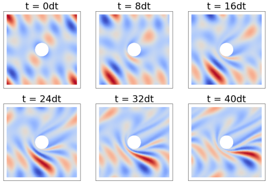
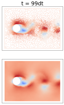
(a) Advection	(b) Incompressible flow

Figure 1: MultiScaleGNN forecasts continuous dynamics. We used it to simulate (a) advection [video] and, (b) the incompressible flow around a circular cylinder [video]. In (a) the upper-lower and left-right boundaries are periodic. In (b) the upper-lower boundaries are periodic. The upper figure shows the $u$ field predicted at a set of nodes obtained with adaptive coarsening/refinement, the bottom figure shows the interpolated field.

Contribution.

We propose MultiScaleGNN, a multi-scale GNN model, to forecast the spatio-temporal evolution of continuous systems discretised as unstructured sets of nodes. Each scale processes the information at different resolutions, enabling the network to more accurately and efficiently capture complex physical systems, such as fluid dynamics, with the same number of learnable parameters as a single level GNN. We apply MultiScaleGNN to simulate two unsteady fluid dynamics problems: advection and incompressible fluid flow around a circular cylinder within the time-periodic laminar vortex-shedding regime. We evaluate the improvement in accuracy over long roll-outs as the number of scales in the model are increased. Importantly, we show that the proposed model is independent of the spatial discretisation and the mean absolute error (MAE) decreases linearly as the distance between nodes is reduced. We exploit this to apply adaptive graph coarsening and refinement. We also demonstrate a technique to impose periodic boundary conditions as an inductive bias on the graph network connectivity. MultiScaleGNN simulations are between two and four orders of magnitude faster than the numerical solver used for generating the ground truth datasets, becoming a potential surrogate model for fast predictions.

2 Background and related work

Deep learning on graphs

A directed graph, $G$, is defined as $G=(V,E)$, where $V=\{1,2,\dots,|V|\}$ is a set of nodes and $E=\{1,2,\dots,|E|\}$ is a set of directed edges, each of them connecting a sender node $s\in V$ to a receiver node $r\in V$. Each node $i$ can be assigned a vector of node attributes $\mathbf{v}_{i}$, and each edge $k$ can be assigned a vector of edge attributes $\mathbf{e}_{k}$. Gilmer, et al. (2017) [16] introduced neural message passing (MP), a layer that updates the node attributes given the current node and edge attributes, as well as a set of learnable parameters. Battaglia et al. (2018) [14] further generalised MP layers by introducing an edge-update function. Their MP layer performs three steps: edge update, aggregation and node update —equations (1), (2) and (3) respectively.

$$\mathbf{e}_{k}^{\prime} =f^{e}(\mathbf{e}_{k},\mathbf{v}_{r_{k}},\mathbf{v}_{s_{k}})\ \ \ \forall k\in E$$ (1)

$$\bar{\mathbf{e}}_{r}^{\prime} =\rho^{e\rightarrow v}(E_{r}^{\prime})\ \ \ \ \ \ \ \ \ \ \ \ \ \forall r\in V$$ (2)

$$\mathbf{v}_{r}^{\prime} =f^{v}(\bar{\mathbf{e}}_{r}^{\prime},\mathbf{v}_{r})\ \ \ \ \ \ \ \ \ \ \ \ \forall r\in V$$ (3)

Functions $f^{e}$ and $f^{v}$ are the edge and node update functions —typically multi-layer perceptrons (MLPs). The aggregation function $\rho^{e\rightarrow v}$ is applied to each subset of updated edges going to node $r$, and it must be permutation invariant. This MP layer has already proved successful in a range of data-driven physics problems [5, 17, 18].

CNNs for simulating continuous mechanics.

During the last five years, most of the DNNs used for predicting continuous physics have included convolutional layers. For instance, CNNs have been used to solve the Poisson’s equation [19, 20], to solve the steady N-S equations [6, 7, 8, 9, 21], and to simulate unsteady fluid flows [4, 10, 12, 22, 23, 24]. These CNN-based solvers are between one and four orders of magnitude faster than numerical solvers [6, 12], and some of them have shown good extrapolation to unseen domain geometries and initial conditions [9, 12].

Simulating physics with GNNs.

Recently, GNNs have been used to simulate the motion of discrete systems of solid particles [18, 25, 26] and deformable solids and fluids discretised into lagrangian (or free) particles [5, 27, 28, 29]. Battaglia, et al. (2016) [18] and Chang, et al. (2016) [25] represented systems of particles as graphs, whose nodes encode the state of the particles and whose edges encode their pairwise interactions; nodes and edges are individually updated through a single MP layer to determine the evolution of the system. Of note is the work of Sanchez, et al. (2020), who discretised fluids into a set of free particles in order to apply the previous approach and infer fluid motion. Further research in this area introduced more general MP layers [26, 29, 30], high-order time-integration [31] and hierarchical models [27, 28]. To the best of our knowledge Alet, et al. (2019) [32] were the first to explore the use of GNNs to infer Eulerian mechanics by solving the Poisson PDE. However, their domains remained simple, used coarse spatial discretisations and did not explore the generalisation of their model. Later, Belbute-Peres, et al. (2020) [33] introduced an hybrid model consisting of a numerical solver providing low-resolution solutions to the N-S equations and several MP layers performing super-resolution on them. More closely related to our work, Pfaff, et al. (2020) [17] proposed a mesh-based GNN to simulate continuum mechanics, although they did not consider the use of MP at multiple scales of resolution.

3 Model

3.1 Model definition

MultiScaleGNN infers the temporal evolution of an $n$-dimensional field, $\mathbf{u}(t,\mathbf{x})\in\mathbb{R}^{n}$, in a spatial domain $\mathcal{D}\subset\mathbb{R}^{2}$. It requires the discretisation of $\mathcal{D}$ into a finite set of nodes $V^{1}$, with coordinates $\mathbf{x}^{1}_{i}\in\mathcal{D}$. Given an input field $\mathbf{u}(t_{0},\mathbf{x}_{V^{1}})$, at time $t=t_{0}$ and at the $V^{1}$ nodes, a single evaluation of MultiScaleGNN returns $\mathbf{u}(t_{0}+dt,\mathbf{x}_{V^{1}})$, where $dt$ is a fixed time-step size. Each time-step is performed by applying MP layers in $L$ graphs and between them, as illustrated in Figure 2.

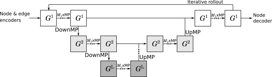
Figure 2: MultiScaleGNN architecture. $G^{1}$ is an original high-resolution graph, $G^{2}$ is a lower-resolution graph obtained from $G^{1}$, $G^{L}$ is the lowest-resolution graph. $M_{l}$ MP layers are applied in each graph, and, DownMP and UpMP layers between them.

The high-resolution graph $G^{1}$ consists of the set of nodes $V^{1}$ and a set of directed edges $E^{1}$ connecting these nodes. In a complete graph there exist $|V^{1}|(|V^{1}|-1)$ edges, however, MP would be extremely expensive. Instead, MultiScaleGNN connects each node in $V^{1}$ (receiver node) to its $k$-closest nodes ($k$-sender nodes) using a k-nearest neighbors (k-NN) algorithm. The node attributes of each node $\mathbf{v}^{1}_{i}$ are the concatenation of $\mathbf{u}(t_{0},\mathbf{x}_{i})$, $\mathbf{p}_{i}$ and $\Omega_{i}$; where $\mathbf{p}_{i}$ is a set of physical parameters at $\mathbf{x}_{i}$ (such as the Reynolds number in fluid dynamics) and

$$\Omega_{i}:=\begin{cases}1&\text{if }\mathbf{x}_{i}\in\partial_{D}\mathcal{D},\\ 0&\text{otherwise},\end{cases}$$ (4)

with $\partial_{D}\mathcal{D}$ representing the Dirichlet boundaries. Each edge attribute $\mathbf{e}^{1}_{k}$ is assigned the relative position between sender node $s_{k}$ and receiver node $r_{k}$. Node attributes and edge attributes are then encoded through two independent MLPs.

A MP layer applied to $G^{1}$ propagates the nodal and edge information only locally between connected (or neighbouring) nodes. Nevertheless, most continuous physical systems require this propagation at larger scales or even globally, for instance, in incompressible flows pressure changes propagate at infinite speed throughout the entire domain. Propagating the nodal and edge attributes between nodes separated by hundreds of hops would necessitate an excessive number of MP layers, which is neither efficient nor scalable. Instead, MultiScaleGNN processes the information at $L$ scales, creating a graph for each level and propagating information between them in each pass. The lower-resolution graphs ($G^{2},G^{3},\dots,G^{L}$; with $|V_{1}|>|V_{2}|>\dots>|V_{L}|$) possess fewer nodes and edges, and hence, a single MP layer can propagate attributes over longer distances more efficiently. These graphs are described in section 3.2. As depicted in Figure 2, the information is first diffused and processed in the high-resolution graph $G^{1}$ through $M_{1}$ MP layers. It is then passed to $G^{2}$ through a downward MP (DownMP) layer. In $G^{2}$ the attributes are again processed through $M_{2}$ MP layers. This process is repeated $L-1$ times. The lowest resolution attributes (stored in $G^{L}$) are then passed back to the scale immediately above through an upward message passing (UpMP) layer. Attributes are successively passed through $M_{l}$ MP layers at scale $l$ and an UpMP layer from scale $l$ to scale $l-1$ until the information is ultimately processed in $G^{1}$. Finally, a MLP decodes the nodal information to return the predicted field at time $t_{0}+dt$ at the $V^{1}$ nodes. To apply MP in the $L$ graphs, MultiScaleGNN uses the MP layer summarised in equations (1) to (3), with the mean as the aggregation function.

3.2 Multi-scale graphs

Each graph $G^{l}=(V^{l},E^{l})$ with $l=2,3,\dots,L$; is obtained from graph $G^{l-1}$ by first dividing $\mathcal{D}$ into a regular grid with cell size $d_{x}^{l}\times d_{y}^{l}$ (Figure 3a exemplifies this for $l=2$). For each cell, provided that there is at least one node from $V^{l-1}$ on it, a node is added to $V^{l}$. The nodes from $V^{l-1}$ on a given cell $i$ and the node from $V^{l}$ on the same cell are denotes as child nodes, $Ch(i)\subset V^{l-1}$, and parent node, $i\in V^{l}$, respectively. The coordinates of each parent node is the mean position of its children nodes. Each edge $k\in E^{l}$ connects sender node $s_{k}\in V^{l}$ to receiver node $r_{k}\in V^{l}$, provided that there exists at least one edge from $Ch(s_{k})$ to $Ch(r_{k})$ in $E^{l-1}$. Edge $k$ is assigned the mean edge attribute of the set of edges going from $Ch(s_{k})$ to $Ch(r_{k})$.

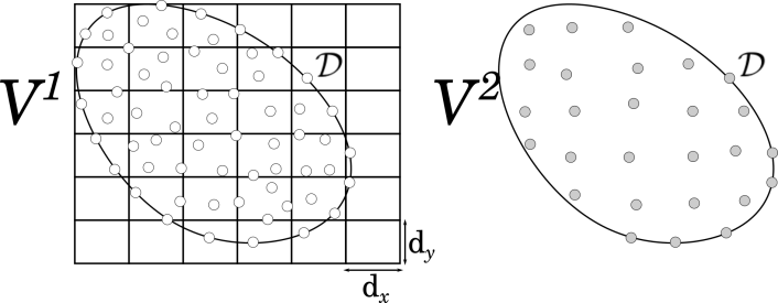
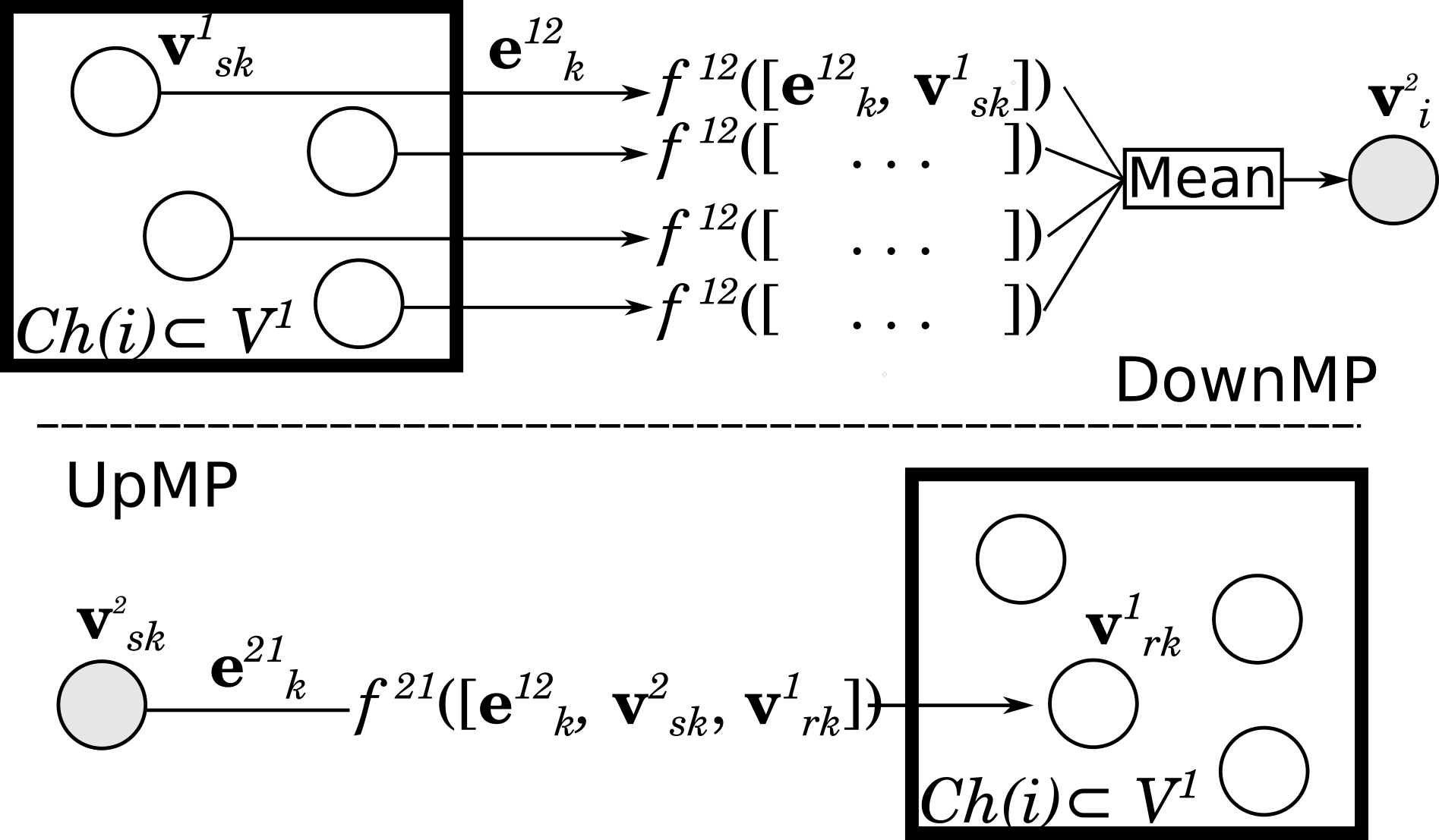
(a) Building $V^{2}$ from $V^{1}$	(b) DownMP and UpMP layers

Figure 3: (a) $V^{2}$ is obtained from $V^{1}$ by partitioning $\mathcal{D}$ using a grid with cell size $d_{x}^{2}\times d_{y}^{2}$ and assigning a parent node $i\in V^{2}$ at the mean position of the child nodes $Ch(i)\subset V^{1}$ in each cell. (b) DownMP and UpMP diagram.

Downward message-passing (DownMP).

To perform MP from $G^{l-1}$ to $G^{l}$ (see Figure 3b), a set of directed edges, $E^{l-1,l}$, is created. Each edge $k\in E^{l-1,l}$ connects node $s_{k}\in V^{l-1}$ to its parent node $r_{k}\in V^{l}$, with edge attributes assigned as the relative position between child and parent nodes. A DownMP layer applies a common edge-update function, $f^{l-1,l}$, to edge $k$ and node $s_{k}$. It then assigns to each node attribute $\mathbf{v}^{l}_{i}$ the mean updated attribute of all the edges in $E^{l-1,l}$ arriving to node $i$, i.e.,

$$\mathbf{v}^{l}_{i}=\frac{1}{|Ch(i)|}\sum_{k:r_{k}=i}f^{l-1,l}([\mathbf{e}^{l-1,l}_{k},\mathbf{v}^{l-1}_{s_{k}}]),\ \ \ \forall i\in 1,\ldots,|V^{l}|.$$ (5)

Upward message-passing (UpMP).

To pass and process the node attributes from $G^{l+1}$ to $G^{l}$, MultiScaleGNN defines a set of directed edges, $E^{l+1,l}$. These edges are the same as in $E^{l,l+1}$, but with opposite direction. An UpMP layer applies a common edge-update function, $f^{l+1,l}$, to each edge $k\in E^{l+1,l}$ and both its sender (at scale $l+1$) and receiver (at scale $l$) nodes, directly updating the node attributes in $G^{l}$, i.e.,

$$\mathbf{v}^{l}_{r_{k}}=f^{l+1,l}([\mathbf{e}^{l+1,l}_{k},\mathbf{v}^{l+1}_{s_{k}},\mathbf{v}^{l}_{r_{k}}]),\ \ \ \forall k\in E^{l+1,l}.$$ (6)

UpMP layers leave the edge attributes of $G^{l}$ unaltered. To model functions $f^{l-1,l}$ and $f^{l+1,l}$ we use MLPs.

3.3 Periodic boundaries

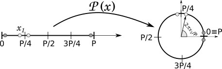
Figure 4: Function $\mathcal{P}$ transforms a periodic direction into a circumference with unitary radius.

MultiLevelGNN imposes periodicity along $x$ and $y$ directions as an inductive bias on $E^{1}$. For this purpose, each periodic direction is transformed through a function $\mathcal{P}:\mathbb{R}\mapsto\mathbb{R}^{2}$ into a circumference with unitary radius,

$$\mathcal{P}(x):=[\cos(2\pi x/P),\sin(2\pi x/P)],$$ (7)

where $P$ is the period along the spatial coordinate under consideration ($x$ or $y$ direction). The k-NN algorithm that creates $E^{1}$ (see Figure 4) is then applied to the transformed coordinates. Even though $E^{1}$ is created based on nodal proximity in the transformed space, the edge attributes are still assigned the relative positions between nodes in the original coordinate system, except at the periodic boundaries where $P$ is added or subtracted to ensure a consistent representation.

3.4 Model training

MultiScaleGNN was trained by supervising at each time-point the loss $\mathcal{L}$ between the predicted field $\hat{\mathbf{u}}(t,\mathbf{x}^{1}_{V^{1}})$ and the ground-truth field $\mathbf{u}(t,\mathbf{x}^{1}_{V^{1}})$ obtained with a high-order finite element solver. $\mathcal{L}$ includes the mean-squared error (MSE) at the $V^{1}$ nodes, the MAE at the $V^{1}$ nodes on Dirichlet-boundaries, and the MSE for the rate of change along the $E^{1}$ edges. $\mathcal{L}$ can be expressed as

$$\mathcal{L}=\mathrm{MSE} \Big{(}\hat{\mathbf{u}}(t,\mathbf{x}^{1}_{V^{1}}),\mathbf{u}(t,\mathbf{x}^{1}_{V^{1}})\Big{)}$$

$$+\lambda_{d}\,\mathrm{MAE}\Big{(}\hat{\mathbf{u}}(t,{\mathbf{x}^{1}_{V^{1}}\in\partial_{D}\mathcal{D}}),\mathbf{u}(t,\mathbf{x}^{1}_{V^{1}}\in\partial_{D}\mathcal{D})\Big{)}$$

$$+\frac{\lambda_{e}}{|E^{1}|}\sum_{\forall k\in E^{1}}\mathrm{MSE}\bigg{(}\frac{\hat{\mathbf{u}}(t,\mathbf{x}^{1}_{r_{k}})-\hat{\mathbf{u}}(t,\mathbf{x}^{1}_{s_{k}})}{||\mathbf{e}_{k}||_{2}},\frac{\mathbf{u}(t,\mathbf{x}^{1}_{r_{k}})-\mathbf{u}(t,\mathbf{x}^{1}_{s_{k}})}{||\mathbf{e}_{k}||_{2}}\bigg{)}.$$ (8)

The hyper-parameters $\lambda_{d}$ and $\lambda_{e}$ are selected based on the physics to be learnt. Training details for our experiments can be found in Appendix B.

4 Training datasets

We generated datasets to train MultiScaleGNN to simulate advection and incompressible fluid dynamics.

Advection.

Datasets AdvBox and AdvInBox contain simulations of a scalar field advected under a uniform velocity field (with magnitude in the range 0 to 1) on a square domain ($[0,1]\times[0,1]$) and a rectangular domain ($[0,1]\times[0,0.5]$) respectively. AdvBox domains have periodic conditions on all four boundaries, whereas AdvInBox domains have upper and lower periodic boundaries, a prescribed Dirichlet condition on the left boundary, and a zero-Neumann condition on the right boundary. The initial states at $t_{0}$ are derived from two-dimensional truncated Fourier series with random coefficients and a random number of terms. For each dataset, a new set of nodes $V^{1}$ is generated at the beginning of every training epoch. For advection models, $\mathbf{u}(t,\mathbf{x}_{i})\in\mathbb{R}$ is the advected field and $\mathbf{p}_{i}(\mathbf{x}_{i})\in\mathbb{R}^{2}$ are the two components the velocity field.

Incompressible fluid dynamics.

Dataset NS contains simulations of the periodic vortex shedding around a circular cylinder at Reynolds number $\mathrm{Re}\in[500,1000]$. The upper and lower boundaries are periodic, hence, the physical problem is equivalent to an infinite vertical array of cylinders. The distance between cylinders, $H$, is randomly sampled between $4$ and $6$. Each domain is discretised into approximately 7000 nodes. For flow models, $\mathbf{u}(t,\mathbf{x}_{i})\in\mathbb{R}^{3}$ contains the velocity and pressure fields and $\mathbf{p}_{i}\in\mathbb{R}$ is the Reynolds number. Further details of the training and testing datasets are included in Appendix A.

5 Results and discussion

We analyse the generalisation to unseen physical parameters, the effect of the number of scales and the independence to the spatial discretisation. All the results, except Tables 1 and 2, were obtained with 3-scale models. Model details and hyper-parameters are included in Appendix B..

Generalisation.

We first consider the MultiScaleGNN model trained to infer advection. Despite MultiScaleGNN being trained on square and rectangular domains and uniform velocity fields, it generalises to complex domains and non-uniform velocity fields (obtained using the N-S equations with $Re=1$). As an example of a closed domain, we consider the Taylor-Couette flow in which the inner and outer boundaries rotate at different speeds. Figure 5a shows the ground truth and predictions for a simulation where the inner wall is moving faster than the outer wall in an anti-clockwise direction. In the Taylor-Couette flow, the structures present in the advected field increase in spatial frequency with time due to the shear flow. This challenges both the networks ability to capture accurate solutions as well as its ability to generalise. After 49 time-steps, the model maintains high accuracy in transporting both the lower and the higher frequencies. We attribute this to the model’s ability to process both high and low resolutions and the frequency range included in the training datasets —training datasets missing high-frequency structures resulted in a considerably higher diffusion.

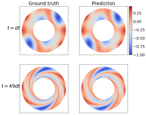
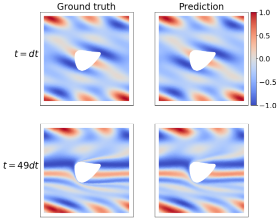
(a) Advection in a Taylor-Couette flow	(b) Advection around a body made of splines

Figure 5: Ground truth and MultiScaleGNN predictions for (a) the advection of scalar field in a Taylor-Couette flow [video], and (b) the advection around a body made of splines with periodicity along $x$ and $y$ [video].

We also evaluate the predictions of MultiScaleGNN on open domains containing obstacles of different shapes (circles, squares, ellipses and closed spline curves). Figure 5b shows the ground truth and predictions for a field advected around a body made of arbitrary splines, with upper-lower and left-right periodic boundaries. The predictions show a strong resemblance to the ground truth, although after 49 time-steps we note that the predicted fields begin to show a higher degree of diffusion in the wake behind the obstacle.

(a)

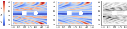
(b)

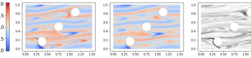
Figure 6: Ground truth and MultiScaleGNN predictions for the advected field after 99 time-steps pass (a) squared and circular obstacles [video], (b) circular obstacles [video]. Upper-lower and left-right boundaries are periodic.

We also assess the quality of long-term inference. Figures 6a and 6b show the ground truth and predictions after 99 time-steps for two obstacles with periodicity in the $x$ and $y$ directions. It can be seen that MultiScaleGNN successfully generalises to infer advection around multiple obstacles. However, the MAE increased approximately linearly every time-step. This limitation could be explained by the simplicity of the training datasets, and it could be mitigated by training on non-uniform velocity fields.

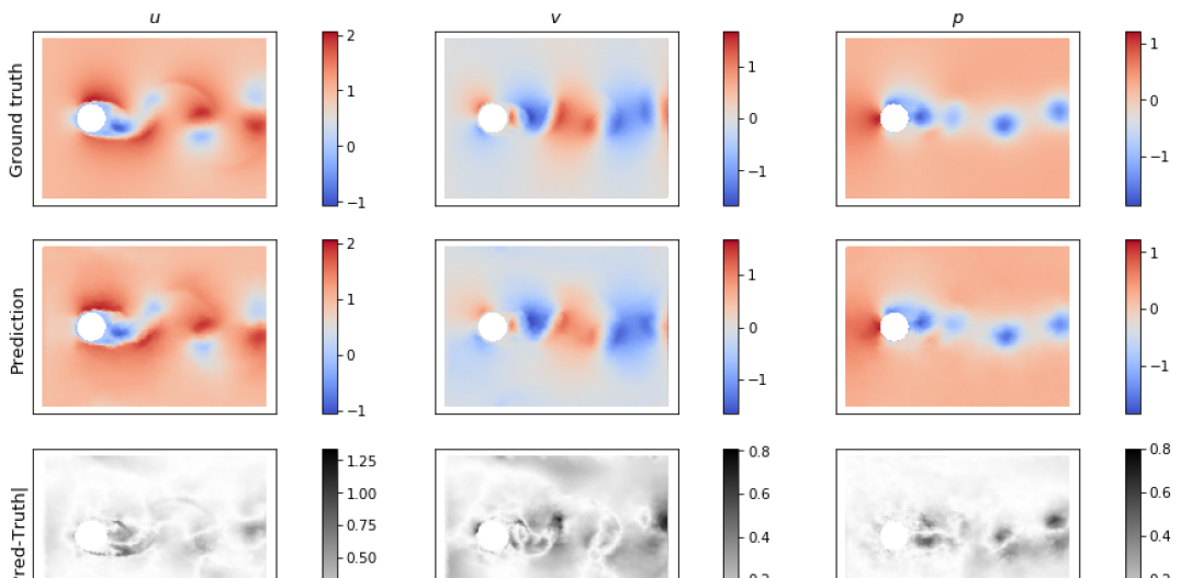
Figure 7: Ground truth and MultiScaleGNN predictions for the horizontal velocity field, $u$, vertical velocity field, $v$, and pressure field, $p$, after 99 time-steps for $\mathrm{Re}=700$ [video].

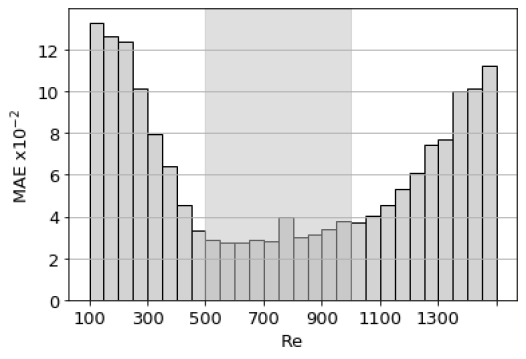
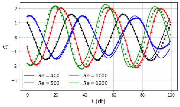
(a) Reynolds vs MAE	(b) Lift coefficient

Figure 8: (a) MAE over 99 time-points for different Reynolds numbers. The grey region indicates the interpolation region. (b) Lift coefficient for $\mathrm{Re}=400,500,1000,1200$. The continuos lines are the ground truth, whereas the dotted lines are the predictions.

MultiScaleGNN was also trained to simulate unsteady incompressible fluid dynamics in a range of Reynolds numbers between 500 and 1000. It shows very good interpolation to unseen Reynolds numbers within this range. For instance, Figure 7 compares the ground truth and predicted fields after 99 time-steps for $\mathrm{Re}=700$. The MAE increases for Reynolds numbers lower than 400 and higher than 1200, as illustrated in Figure 8a, which represents the MAE for a range of Reynolds numbers between 100 and 1500. Figure 8b shows the temporal evolution of the lift coefficient (vertical component of the integral of the pressure forces on the cylinder walls) for simulations with $\mathrm{Re}=400,500,1000$ and $1200$ (with $H=5$). It can be noticed that for $\mathrm{Re}=500$ and $1000$, both at the edge of our training range, the ground truth (continuous lines) and the predictions (dotted lines) match very well over the entire simulation time. For $\mathrm{Re}=400$ and $1200$ the lift predictions are qualitatively correct but begin to differ slightly in amplitude and phase. The reason for the limited extrapolation may be the complexity of the N-S equations, which result into shorter wakes and higher frequencies as the Reynolds number is increased.

Multiple scales.

We evaluate the accuracy of MultiScaleGNN with $L=1,2,3$ and $4$; the architectural details of each model are included in Appendix B. Tables 1 and 2 collect the MAE for the last time-point and the mean of all the time-points on the testing datasets. Incompressible fluids have a global behaviour since pressure waves travel at an infinite speed. The addition of coarser layers helps the network learn this characteristic and achieve significantly lower errors. For dataset NSMidRe, within the training regime of $\mathrm{Re}$, and NSHighRe there is a clear benefit from using four scales. Interestingly, dataset NSLowRe shows a clear gain only when using two levels. This may be in part due to this dataset being in the extrapolation regime of $\mathrm{Re}$.

In contrast, for the advection datasets, the MAE does not substantially decrease when using an increasing number of levels. In advection, information is propagated only locally and at a finite speed. However, an accurate advection model must guarantee that it propagates the nodal information at least as fast as the velocity field driving the advection, similar to the Courant–Friedrichs–Lewy (CFL) condition used in numerical analysis. In MultiScaleGNN, the coarser graphs help to satisfy this condition, while the original graph maintains a detailed representation of structures in the advected fields. Thus, GNNs for simulating both global and local continuum physics can benefit from learning information at multiple scales. As a comparison to Pfaff, et al. (2020) [17], a GNN with 16 sequential MP-layers (GN-Blocks) results in a MAE of $5.852\times 10^{-2}$ on our NSMidRe dataset; whereas MultiScaleGNN with the same number and type of MP layers, but distributed among 3 scales, results in a lower MAE of $3.201\times 10^{-2}$.

Table 1: MAE $\times 10^{-2}$ on the advection testing sets for MultiScaleGNN models with $L=1,2,3,4$

Datasets	$L=1$		$L=2$		$L=3$		$L=4$
	Step 49	All	Step 49	All	Step 49	All	Step 49	All
AdvTaylor	7.794	3.661	7.055	3.157	7.424	3.355	7.626	3.441
AdvCircle	3.508	1.758	3.119	1.547	2.986	1.475	3.486	1.629
AdvCircleAng	3.880	1.923	3.618	1.762	3.464	1.689	3.493	1.690
AdvSquare	3.765	1.853	3.493	1.689	3.279	1.571	3.219	1.556
AdvEllipseH	3.508	1.758	3.119	1.547	2.986	1.475	3.486	1.629
AdvEllipseV	3.770	1.867	3.748	1.853	3.450	1.708	3.334	1.653
AdvSplines	4.021	1.957	3.960	1.876	3.720	1.758	3.599	1.705
AdvInCir	9.886	6.008	10.755	6.298	14.948	8.491	9.670	5.808

Table 2: MAE $\times 10^{-2}$ on the N-S testing sets for MultiScaleGNN models with $L=1,2,3,4$

Datasets	$L=1$		$L=2$		$L=3$		$L=4$
	Step 99	All	Step 99	All	Step 99	All	Step 99	All
NSMidRe	13.028	8.033	4.731	3.666	3.95	3.201	3.693	3.032
NSLowRe	12.056	8.193	9.756	6.861	11.058	7.466	11.556	7.603
NSHighRe	16.176	11.42	9.949	7.385	8.936	7.17	9.085	6.822

Discretisation independence.

MultiScaleGNN processes the relative position between neighbouring nodes, but it does not consider the absolute position of nodes. It was also trained with random node distributions for each training example. This ensures MultiScaleGNN is independent to the set of nodes $V^{1}$ chosen to discretise the physical domain. To demonstrate this, we consider a simulation from the AdvCircleAng dataset (see Figure 1a). Figure 9a shows the MAE for a number of $V^{1}$ sets, with nodes evenly distributed on the domain. It can be seen that the MAE decreases linearly as the mean distance-to-neighbour is reduced – at least within the interval shown. Figure 9a also shows how the inference time per time-step increases exponentially as the spatial resolution is increased. For this reason, the $V^{1}$ sets we feed to MultiScaleGNN include a higher node count around solid walls. As an example, the nodes $V^{1}$ used for the simulation depicted in Figure 1a are represented in Figure 9b.

(a)

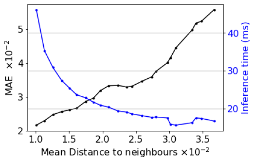
(b)

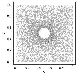
Figure 9: (a) For sample in Figure 1a., the MAE over 49 time-points and the inference time per time-step for a number of quasi-uniform discretisations. (b) $V^{1}$ nodes used for the simulation shown in Figure 1a.

Adaptive remeshing is a technique used by numerical solvers to ensure sufficient resolution is present where needed in the computational domain. It dynamically modifies the spatial discretisation at every time-step. Likewise, we implemented an algorithm to locally increase or decrease the spatial resolution of $V^{1}$ before every model evaluation. Our algorithm increases the node count where the gradients of $\mathbf{u}$ are higher and decreases it where these are lower. Figure 1b shows the $u$ field predicted by MultiScaleGNN combined with this technique. It can be seen that the resolution is reduced far from the wake and increased close to the cylinder walls and on the vortices travelling downstream. Adaptive coarsening/refinement allowed us to achieved an 11% reduction of the MAE at the 99${}^{\text{th}}$ time-point on the NSMidRe dataset. More details are included in Appendix C.

Computational efficiency.

We compare MultiScaleGNN and the spectral/$hp$ element numerical solver [2] used for generating the training and testing datasets. For advection, MultiScaleGNN simulations are one order of magnitude faster when they run on a CPU, and almost three orders of magnitude faster on a GPU. The inference time per time-step for AdvTaylor is around 30 ms, and around 90 ms for the remaining testing datasets on a Tesla T4 GPU. For the N-S equations, MultiScaleGNN achieves an speed-up of three orders of magnitude running on a CPU, and four orders of magnitude on a Tesla T4 GPU; with an inference time per time-step of 50 ms on a Tesla T4 GPU.

6 Conclusion

MultiScaleGNN is a novel multi-scale GNN model for inferring mechanics on continuous systems discretised into unstructured sets of nodes. Unstructured discretisations allow complex domains to be accurately represented and the node count to be adjusted over space. Multiple coarser levels allow high and low-resolution mechanics to be efficiently captured. For spatially local problems, such as advection, MP layers in coarse graphs guarantee that the information is diffused at the correct speed while MP layers in finer graphs provide sharp resolution of the fields. In global and local problems, such as incompressible fluid dynamics, the coarser graphs are particularly advantageous, since they enable global characteristics such as pressure waves to be effectively learnt. MultiScaleGNN interpolates to unseen spatial discretisations of the physical domains, allowing it to adopt efficient discretisations and to dynamically and locally modify them to further improve the accuracy. MultiScaleGNN also generalises to advection on complex domains and velocity fields and it interpolates to unseen Reynolds numbers in fluid dynamics. Inference is between two and four orders of magnitude faster than with the high-order solver used for generating the training datasets. This work is a significant advancement in the design of flexible, accurate and efficient neural simulators.

Appendix A Datasets details

A.1 Advection datasets

We solved the two-dimensional advection equation using Nektar++, an spectral/hp element solver [1, 2]. The advection equation reads

$$\frac{\partial\varphi}{\partial t}+u(x,y)\frac{\partial\varphi}{\partial x}+v(x,y)\frac{\partial\varphi}{\partial y}=0,$$ (9)

where $\varphi(t,x,y)$ is the advected field, and, $u$ and $v$ are the horizontal and vertical components of the velocity field respectively. As initial condition, $\varphi_{0}$, we take an scalar field derived from a two-dimensional Fourier series with $M\times N$ random coefficients, specifically

$$\varphi_{0}=\sum_{m=0}^{M}\sum_{n=0}^{N}c_{m,n}\varphi_{m,n}\cdot\exp\Big{(}-2(x-x_{c})^{2}-2(x-x_{c})^{2}\Big{)},$$ (10)

$$\text{with}\ \ \ \varphi_{m,n}=\Re\bigg{\{}\exp\Big{(}i2\pi(mx+ny)\Big{)}\bigg{\}}.$$ (11)

Coefficients $c_{m,n}$ are sampled from a uniform distribution between 0 and 1, and, integers $M$ and $N$ are randomly selected between 3 and 8. In equation (11), $x_{c}$ and $y_{c}$ are the coordinates of the centre of the domain. The initial field $\varphi_{0}$ is scaled to have a maximum equal to $1$ and a minimum equal to $-1$. Figure 10a shows an example of $\varphi_{0}$ with $M=5$ and $N=7$ on a squared domain. We created training and testing datasets containing advection simulations with 50 time-points each, equispaced by a time-step size $dt=0.03$. A summary of these datasets can be found in Table 3.

(a)

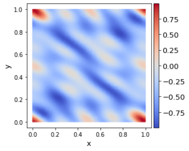
(b)

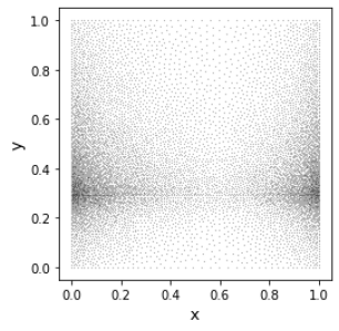
Figure 10: (a) Initial condition with with $M=5$ and $N=7$ from the AdvBox dataset. (b) One of the sets of nodes $V^{1}$ used during training.

Training datasets.

We generated two training datasets: AdvBox with 1500 simulations and AdvInBox with 3000 simulations. In these datasets we impose a uniform velocity fields with random values for $u$ and $v$, but constrained to $u^{2}+v^{2}\leq 1$. In dataset AdvBox the domain is a square ($\mathbf{x}\in[0,1]\times[0,1]$) with periodicity in $x$ and $y$. In dataset AdvInBox the domain is a rectangle ($\mathbf{x}\in[0,1]\times[0,0.5]$) with periodicity in $y$, a Dirichlet condition on the left boundary and a homogeneous Neumann condition on the right boundary – as an additional constraint, $u\geq 0$. During training, a new set of nodes $V^{1}$ is selected at the beginning of every epoch. The node count was varied smoothly across the different regions of the domains, as illustrated in Figure 10b. The sets of node were created with Gmsh, a finite-element mesher. The element size parameter was set to 0.012 in the corners and the centre of the training domains, and set to $\sqrt{10}$ and $1/\sqrt{10}$ times that value at one random control point on each boundary. The mean number of nodes in the AdvBox and AdvInBox datasets are 98002 and 5009 respectively.

Testing datasets.

We generated eight testing datasets, each of them containing 200 simulations. These datasets consider advection on more complex open and closed domains with non-uniform velocity fields. The domains employed are represented in Figure 11, and the testing datasets are listed in Table 3. The velocity fields were obtained from the steady incompressible Navier-Stokes equations with $Re=1$. In dataset AdvTaylor the inner and outer walls spin at a velocity randomly sampled between $-1$ and $1$. In datasets AdvCircle, AdvSquare, AdvEllipseH, AdvEllipseV and AdvSplines there is periodicity along $x$ and $y$, and a horizontal flow rate between $0.2$ and $0.75$ is imposed. The obstacles inside the domains on the AdvSplines dataset are made of closed spline curves defined from six random points. Dataset AdvCircleAng is similar to AdvCircle, but the flow rate forms an angle between $-45\deg$ and $45\deg$ with the $x$ axis. The domain in dataset AdvInCir has periodicity along $y$, a Dirichlet condition on the left boundary (with $0.2\leq u^{2}+v^{2}\leq 0.75$ and $-45\deg\leq\arctan(v/u)\leq 45\deg$), and a homogeneous Neumann condition on the right boundary. The set of nodes $V^{1}$ were generated using Gmsh with an element size equal to 0.005 on the walls of the obstacles and 0.01 on the remaining boudaries.

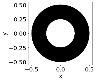
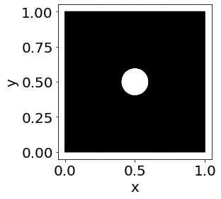
(a) (b) (c) (d) (e) (f)

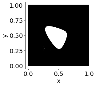
Figure 11: Physical domains (black areas) on our testing datasets.

Table 3: Advection training and testing datasets

Dataset	Flow type	Domain	#Nodes	Train/Test
AdvBox	Open, periodic in $x$ and $y$	$[0,1]\times[0,1]$	9601-10003	Training
AdvInBox	Open, periodic in $y$	$[0,1]\times[0,0.5]$	4894-5135	Training
AdvTaylor	Closed, Taylor-Couette flow	Figure 11a	7207	Testing
AdvCircle	Open, periodic in $x$ and $y$	Figure 11b	19862	Testing
AdvCircleAng	Open, periodic in $x$ and $y$	Figure 11b	19862	Testing
AdvSquare	Open, periodic in $x$ and $y$	Figure 11c	19956	Testing
AdvEllipseH	Open, periodic in $x$ and $y$	Figure 11d	20210	Testing
AdvEllipseV	Open, periodic in $x$ and $y$	Figure 11e	20221	Testing
AdvSplines	Open, periodic in $x$ and $y$	Figure 11f	19316-20389	Testing
AdvIncir	Open, periodic in $y$	Figure 11b	19862	Testing

A.2 Incompressible fluid dynamics datasets

We solved the two-dimensional incompressible Navier-Stokes equation using the high-order solver Nektar++. The Navier-Stokes equations read

$$\frac{\partial u}{\partial x}+\frac{\partial v}{\partial y}=0,$$ (12)

$$\frac{\partial u}{\partial t}+u\frac{\partial u}{\partial x}+v\frac{\partial u}{\partial y}=-\frac{\partial p}{\partial x}+\frac{1}{Re}\bigg{(}\frac{\partial^{2}u}{\partial x^{2}}+\frac{\partial^{2}u}{\partial y^{2}}\bigg{)},$$ (13)

$$\frac{\partial v}{\partial t}+u\frac{\partial v}{\partial x}+v\frac{\partial v}{\partial y}=-\frac{\partial p}{\partial y}+\frac{1}{Re}\bigg{(}\frac{\partial^{2}v}{\partial x^{2}}+\frac{\partial^{2}v}{\partial y^{2}}\bigg{)},$$ (14)

where $u(t,x,y)$ and $v(t,x,y)$ are the horizontal and vertical components of the velocity field, $p(t,x,y)$ is the pressure field, and $Re$ is the Reynolds number. We consider the flow around an infinite vertical array of circular cylinder, with diameter $D=1$, equispaced a distance $H$ randomly sampled between $4D$ and $6D$. The width of the domain is $7D$ and the cylinders axis is at $1.5D$ from the left boundary. The left boundary is an inlet with $u=1$, $v=0$ and $\partial p/\partial x=0$; the right boundary is an outlet with $\partial u/\partial x=0$, $\partial v/\partial x=0$ and $p=0$; and, the cylinder walls have a no-slip condition. The numerical solutions obtained for this flow at different Reynolds numbers are well known [34]. In our simulations we select $Re$ values that yield solutions in the laminar vortex-shedding regime, and we only include the periodic stage. The sets of nodes $V^{1}$ employed for each simulation were created using Gmsh placing more nodes around the cylinders walls (see Figure 12a). The mean number of nodes in these sets is 7143. Each simulation contains $100$ time-points equispaced by a time-step size $dt=0.1$. The training and testing datasets are listed in Table 4.

Table 4: Incompressible flow training and testing datasets

Dataset	$Re$	#Simulations	Train/Test
NS	500-1000	1000	Training
NSMidRe	500-1000	250	Testing
NSLowRe	100-500	250	Testing
NSMidRe	1000-1500	250	Testing

Appendix B Model details

Hyper-parameters choice.

MultiScaleGNN’s hyper-parameters have different values for advection models and fluid dynamics models, Table 5 collects the values we employed. All MLPs use SELU activation functions [35], and, batch normalisation [36]. Our results (except results in Tables 1 and 2) were obtained with $L=3$, and, $M_{1}=2$, $M_{2}=2$, $M_{3}=4$ for advection; and $M_{1}=4$, $M_{2}=3$, $M_{3}=2$ for fluid dynamics.

Table 5: MultiScaleGNN details

Hyper-parameters	Advection	Fluid dynamics
$k$	4	8
$d_{x}^{2},d_{y}^{2}$	0.02	0.15
$d_{x}^{3},d_{y}^{3}$	0.04	0.30
$d_{x}^{4},d_{y}^{4}$	0.08	0.60
#Layers in edge encoder	2	2
#Layers in node encoder	2	2
#Layers in node decoder	2	2
#Layers in edge MLPs	2	3
#Layers in node MLPs	2	2
#Layers in DownMP MLPs	2	3
#Layers in UpMP MLPs	2	3
#Neurons per layer	128	128

Multi-scale experiments.

The number of MP layers at each scale used for obtaining the results in Tables 1 and 2 are listed in the table below. Notice that the total number of MP layers at each scale $l<L$, is $2\times M_{l}$.

Table 6: $M_{l}$ in the multi-scale experiments

$L$	Advection	Fluid dynamics
$L=1$	$M_{1}=4$	$M_{1}=8$
$L=2$	$M_{1}=2,M_{2}=4$	$M_{1}=4,M_{2}=4$
$L=3$	$M_{1}=2,M_{2}=2,M_{3}=4$	$M_{1}=4,M_{2}=2,M_{3}=4$
$L=4$	$M_{1}=2,M_{2}=2,M_{3}=2,M_{4}=4$	$M_{1}=4,M_{2}=2,M_{3}=2,M_{4}=4$

Training details.

We trained MultiScaleGNN models on a internal cluster using 4 CPUs, 86GB of memory, and a RTX6000 GPU with 24GB. We fed 8 graphs per batch. First, each training iteration predicted a single time-point, and, every time the training loss decreased below a threshold (0.01 for advection and 0.005 for fluid dynamics) we increased the number of iterative time-steps by one, up to a limit of 10. We used the loss function given by equation (8) with $\lambda_{d}=0.25$, and, $\lambda_{e}=0.5$ for advection and $\lambda_{e}=0$ for fluid dynamics. The initial time-point was randomly selected for each prediction, and, we added to the initial field noise following a uniform distribution between -0.01 and 0.01. After each time-step, the models’ weights were updated using the Adam optimiser with its standard parameters [37]. The learning rate was set to $10^{-4}$ and multiplied by 0.5 when the training loss did not decrease after five consecutive epochs, also, we applied gradient clipping to keep the Frobenius norm of the weights gradients below or equal to one.

Appendix C Adaptive coarsening/refinement

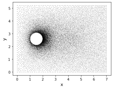
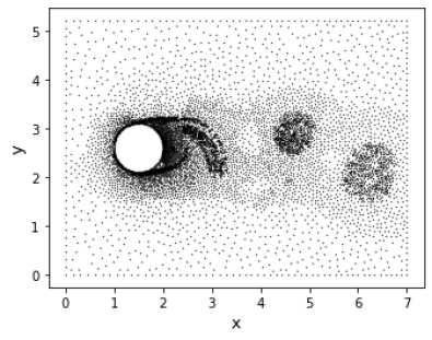
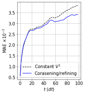
(a) Original $V^{1}$	(b) Coarsened/refined $V^{1}$ at time $t$	(c) MAE

Figure 12: (a) Original set of nodes and (b) set of nodes after applying our coarsening/refinement algorithm with $c=0.4$ and $f=0.1$. (c) MAE on the NSMidRe dataset for MultiScaleGNN without adaptive coarsening/refinement and MultiScaleGNN combined with our coarsening/refinement algorithm.

We implemented an algorithm to locally coarsen and refine the sets of nodes inputted to MultiScaleGNN based on the gradients of the fields at these nodes. The input to the coarsening/refinement algorithm is a set of nodes $V^{1}$, and the output is the same set with some of its nodes removed and some new nodes added to it. The coarsening happens in regions where the amount of nodes is more than enough to capture the spatial variations of the input field, whereas the refinement happens in regions where more resolution is required. The algorithm begins by connecting each node to its $k$-closest nodes, we denote the resulting set of edges by $E^{c/f}$. Then, $\overline{\Delta u}$ is computed at each node. We define $\overline{\Delta u}$ as

$$\Delta u_{k} :=||\mathbf{u}(t,\mathbf{x}_{r_{k}})-\mathbf{u}(t,\mathbf{x}_{s_{k}})||_{2}\ \ \ \forall k\in E^{c/f},$$ (15)

$$\overline{\Delta u}_{i} :=\sum_{k:r_{k}=i}\Delta u_{k}\ \ \ \ \ \ \ \ \ \ \ \ \ \ \ \ \ \ \ \ \ \ \ \ \ \forall i\in V^{1},$$ (16)

and, it summarises the mean magnitude of the gradients of field $\mathbf{u}$ at each node.

The set of nodes $V^{1}_{c}$, which contains the nodes with a value of $\overline{\Delta u}$ below the $c|V^{1}|^{\text{th}}$-lowest value, is applied a coarsening algorithm; whereas the set of nodes $V^{1}_{f}$, which contains the nodes with a value above the $f|V^{1}|^{\text{th}}$-highest, is applied a refinement algorithm. Values $c$ and $f$ can be chosen depending on the performance requirements. The coarsening is based on Guillard’s coarsening [38], and, it consists on removing the $k$-closest nodes to node $i\in V^{1}_{c}$ provided that node $i$ has not been removed yet. The refinement algorithm we implemented can be interpreted as an inverse of Guillard’s coarsening: for each node $i\in V^{1}_{f}$, $k$ triangles with node $i$ and its $k$-closest nodes at their vertices are created, then, new nodes are added at the centroids of those triangles. Figure 12a shows an example of a set of nodes provided to our coarsening/refinement algorithm, and Figure 12b shows the resulting set of nodes for $c=0.4$ and $f=0.1$. Notice that, in line with Guillard’s coarsening, the nodes on the boundaries of the domain are not considered by our algorithm. We trained MultiScaleGNN on the NS dataset with sets of nodes obtained for $c$ between 0.3 and 0.5, and $f$ between 0.05 and 0.15. Then, during inference time, the sets of nodes $V^{1}$ fed to MultiScaleGNN are coarsened/refined before every time-step. Figure 12c compares the MAE on the NSMidRe dataset for MultiScaleGNN without adaptive coarsening/refinement and MultiScaleGNN combined with our coarsening/refinement algorithm. For a fair comparison, adaptive-MultiScaleGNN predictions are interpolated to the primitive set of nodes, and the MAEs for both models are computed in the same set of nodes. From this figure, it is clear, that having the ability to dynamically adapt the resolution can help to further improve the long-term accuracy.

References

- [1] George Karniadakis and Spencer Sherwin. Spectral/hp element methods for computational fluid dynamics. Oxford University Press, 2013.
- [2] Chris D Cantwell, David Moxey, Andrew Comerford, Alessandro Bolis, Gabriele Rocco, Gianmarco Mengaldo, Daniele De Grazia, Sergey Yakovlev, J-E Lombard, Dirk Ekelschot, et al. Nektar++: An open-source spectral/hp element framework. Computer physics communications, 192:205–219, 2015.
- [3] Jonathan Tompson, Kristofer Schlachter, Pablo Sprechmann, and Ken Perlin. Accelerating eulerian fluid simulation with convolutional networks. In International Conference on Machine Learning, pages 3424–3433. PMLR, 2017.
- [4] Byungsoo Kim, Vinicius C Azevedo, Nils Thuerey, Theodore Kim, Markus Gross, and Barbara Solenthaler. Deep fluids: A generative network for parameterized fluid simulations. In Computer Graphics Forum. Wiley Online Library, 2019.
- [5] Alvaro Sanchez-Gonzalez, Jonathan Godwin, Tobias Pfaff, Rex Ying, Jure Leskovec, and Peter Battaglia. Learning to simulate complex physics with graph networks. In International Conference on Machine Learning, pages 8459–8468. PMLR, 2020.
- [6] Xiaoxiao Guo, Wei Li, and Francesco Iorio. Convolutional neural networks for steady flow approximation. In Proceedings of the 22nd ACM SIGKDD international conference on knowledge discovery and data mining, pages 481–490, 2016.
- [7] Emre Yilmaz and Brian German. A convolutional neural network approach to training predictors for airfoil performance. In 18th AIAA/ISSMO multidisciplinary analysis and optimization conference, page 3660, 2017.
- [8] Yao Zhang, Woong Je Sung, and Dimitri N Mavris. Application of convolutional neural network to predict airfoil lift coefficient. In 2018 AIAA/ASCE/AHS/ASC Structures, Structural Dynamics, and Materials Conference, page 1903, 2018.
- [9] Nils Thuerey, Konstantin Weissenow, Lukas Prantl, and Xiangyu Hu. Deep Learning Methods for Reynolds-Averaged Navier-Stokes Simulations of Airfoil Flows. AIAA Journal, 58(1):15–26, oct 2018.
- [10] Steffen Wiewel, Moritz Becher, and Nils Thuerey. Latent space physics: Towards learning the temporal evolution of fluid flow. In Computer Graphics Forum. Wiley Online Library, 2019.
- [11] Xiangyun Xiao, Yanqing Zhou, Hui Wang, and Xubo Yang. A novel cnn-based poisson solver for fluid simulation. IEEE transactions on visualization and computer graphics, 26(3):1454–1465, 2018.
- [12] Mario Lino, Chris Cantwell, Stathi Fotiadis, Eduardo Pignatelli, and Anil Anthony Bharath. Simulating surface wave dynamics with convolutional networks. In NeurIPS Workshop on Interpretable Inductive Biases and Physically Structured Learning, 2020.
- [13] Ian Goodfellow, Yoshua Bengio, Aaron Courville, and Yoshua Bengio. Deep learning. MIT press Cambridge, 2016.
- [14] Peter W Battaglia, Jessica B Hamrick, Victor Bapst, Alvaro Sanchez-Gonzalez, Vinicius Zambaldi, Mateusz Malinowski, Andrea Tacchetti, David Raposo, Adam Santoro, Ryan Faulkner, et al. Relational inductive biases, deep learning, and graph networks. arXiv preprint arXiv:1806.01261, 2018.
- [15] Zonghan Wu, Shirui Pan, Fengwen Chen, Guodong Long, Chengqi Zhang, and S Yu Philip. A comprehensive survey on graph neural networks. IEEE Transactions on Neural Networks and Learning Systems, 2020.
- [16] Justin Gilmer, Samuel S. Schoenholz, Patrick F. Riley, Oriol Vinyals, and George E. Dahl. Neural message passing for quantum chemistry. In 34th International Conference on Machine Learning, ICML 2017, 2017.
- [17] Tobias Pfaff, Meire Fortunato, Alvaro Sanchez-Gonzalez, and Peter W Battaglia. Learning mesh-based simulation with graph networks. In (accepted) 38th International Conference on Machine Learning, ICML 2021, 2021.
- [18] Peter W Battaglia, Razvan Pascanu, Matthew Lai, Danilo Rezende, and Koray Kavukcuoglu. Interaction networks for learning about objects, relations and physics. In 38th Neural Information Processing Systems, NeurIPS 2016, 2016.
- [19] Wei Tang, Tao Shan, Xunwang Dang, Maokun Li, Fan Yang, Shenheng Xu, and Ji Wu. Study on a Poisson’s equation solver based on deep learning technique. 2017 IEEE Electrical Design of Advanced Packaging and Systems Symposium, EDAPS 2017, 2018-Janua:1–3, 2018.
- [20] Ali Girayhan Özbay, Sylvain Laizet, Panagiotis Tzirakis, Georgios Rizos, and Björn Schuller. Poisson CNN: Convolutional Neural Networks for the Solution of the Poisson Equation with Varying Meshes and Dirichlet Boundary Conditions, 2019.
- [21] Tharindu P Miyanawala and Rajeev K Jaiman. A novel deep learning method for the predictions of current forces on bluff bodies. In Proceedings of the ASME 2018 37th International Conference on Ocean, Offshore and Arctic Engineering, June 2018.
- [22] Sangseung Lee and Donghyun You. Data-driven prediction of unsteady flow over a circular cylinder using deep learning. Journal of Fluid Mechanics, 879:217–254, 2019.
- [23] William Sorteberg, Stef Garasto, Alison Pouplin, Chris Cantwell, and Anil A. Bharath. Approximating the Solution to Wave Propagation using Deep Neural Networks. In NeurIPS Workshop on Modeling the Physical World: Perception, Learning, and Control, December 2018.
- [24] Stathi Fotiadis, Eduardo Pignatelli, Mario Lino, Chris Cantwell, Amos Storkey, and Anil A. Bharath. Comparing recurrent and convolutional neural networks for predicting wave propagation. In ICLR Workshop on Deep Neural Models and Differential Equations, 2020.
- [25] Michael B Chang, Tomer Ullman, Antonio Torralba, and Joshua B Tenenbaum. A compositional object-based approach to learning physical dynamics. In 5th International Conference on Learning Representations, ICLR 2017, 2017.
- [26] Alvaro Sanchez-Gonzalez, Nicolas Heess, Jost Tobias Springenberg, Josh Merel, Martin Riedmiller, Raia Hadsell, and Peter Battaglia. Graph networks as learnable physics engines for inference and control. 35th International Conference on Machine Learning, ICML 2018, 10:7097–7117, 2018.
- [27] Yunzhu Li, Jiajun Wu, Russ Tedrake, Joshua B Tenenbaum, and Antonio Torralba. Learning particle dynamics for manipulating rigid bodies, deformable objects, and fluids. In 7th International Conference on Learning Representations, ICLR 2019, 2019.
- [28] Damian Mrowca, Chengxu Zhuang, Elias Wang, Nick Haber, Li F Fei-Fei, Josh Tenenbaum, and Daniel L Yamins. Flexible neural representation for physics prediction. In Advances in neural information processing systems, pages 8799–8810, 2018.
- [29] Yunzhu Li, Jiajun Wu, Jun Yan Zhu, Joshua B. Tenenbaum, Antonio Torralba, and Russ Tedrake. Propagation networks for model-based control under partial observation. Proceedings - IEEE International Conference on Robotics and Automation, 2019-May:1205–1211, 2019.
- [30] Damian Mrowca, Chengxu Zhuang, Elias Wang, Nick Haber, Li Fei-Fei, Joshua B. Tenenbaum, and Daniel L.K. Yamins. Flexible neural representation for physics prediction. Advances in Neural Information Processing Systems, 2018-Decem:8799–8810, 2018.
- [31] Alvaro Sanchez-Gonzalez, Victor Bapst, Kyle Cranmer, and Peter Battaglia. Hamiltonian graph networks with ode integrators. arXiv preprint arXiv:1909.12790, 2019.
- [32] Ferran Alet, Adarsh K Jeewajee, Maria Bauza, Alberto Rodriguez, Tomas Lozano-Perez, and Leslie Pack Kaelbling. Graph element networks: adaptive, structured computation and memory. arXiv preprint arXiv:1904.09019, 2019.
- [33] Filipe de Avila Belbute-Peres, Thomas Economon, and Zico Kolter. Combining differentiable pde solvers and graph neural networks for fluid flow prediction. In International Conference on Machine Learning, pages 2402–2411. PMLR, 2020.
- [34] Hongyi Jiang and Liang Cheng. Large-eddy simulation of flow past a circular cylinder for reynolds numbers 400 to 3900. Physics of Fluids, 33(3):034119, 2021.
- [35] Günter Klambauer, Thomas Unterthiner, Andreas Mayr, and Sepp Hochreiter. Self-normalizing neural networks. arXiv preprint arXiv:1706.02515, 2017.
- [36] Jimmy Lei Ba, Jamie Ryan Kiros, and Geoffrey E Hinton. Layer normalization. arXiv preprint arXiv:1607.06450, 2016.
- [37] Diederik P. Kingma and Jimmy Ba. Adam: A method for stochastic optimization. In Yoshua Bengio and Yann LeCun, editors, 3rd International Conference on Learning Representations, ICLR 2015, San Diego, CA, USA, May 7-9, 2015, Conference Track Proceedings, 2015.
- [38] Hervé Guillard. Node-nested multi-grid method with delaunay coarsening. Technical report, INRIA, 1993.