RealTranS: End-to-End Simultaneous Speech Translation with Convolutional Weighted-Shrinking Transformer
Abstract
End-to-end simultaneous speech translation (SST), which directly translates speech in one language into text in another language in real-time, is useful in many scenarios but has not been fully investigated. In this work, we propose RealTranS, an end-to-end model for SST. To bridge the modality gap between speech and text, RealTranS gradually downsamples the input speech with interleaved convolution and unidirectional Transformer layers for acoustic modeling, and then maps speech features into text space with a weighted-shrinking operation and a semantic encoder. Besides, to improve the model performance in simultaneous scenarios, we propose a blank penalty to enhance the shrinking quality and a Wait-K-Stride-N strategy to allow local reranking during decoding. Experiments on public and widely-used datasets show that RealTranS with the Wait-K-Stride-N strategy outperforms prior end-to-end models as well as cascaded models in diverse latency settings.
1 Introduction
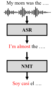
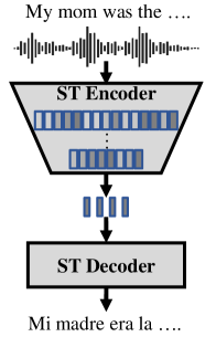
Simultaneous speech translation (SST) Fügen et al. (2007); Oda et al. (2014); Ren et al. (2020) aims to translate speech in one language into text in another language concurrently. It is useful in many scenarios, like synchronous interpretation in international conferences, automatic caption for live videos, etc. However, prior studies either focus on full sentence speech translation (ST) Berard et al. (2016); Weiss et al. (2017); Liu et al. (2019) or simultaneous text-to-text machine translation (STT) Cho and Esipova (2016); Gu et al. (2017); Dalvi et al. (2018) which takes a segmented output from an automatic speech recognition (ASR) system as input. Such two-stage models (i.e., cascaded models) inevitably introduce error propagation and also increase translation latency (see Figure 1). Ren et al. (2020) propose an end-to-end SST system called SimulSpeech, but they ignore the modality gap between speech and text, which is important for improving translation quality Liu et al. (2020).
In this paper, we propose RealTranS model for SST. To relieve the burden of our encoder Wang et al. (2020c); Liu et al. (2020), we decouple it into three parts: acoustic encoder, weighted-shrinking operation, and semantic encoder. We apply Conv-Transformer Huang et al. (2020) as our acoustic encoder, which gradually downsamples the input speech and learns acoustic information with interleaved convolution and Transformer layers. The weighted-shrinking operation bridges the length gap between speech and text, by weighted summing up the frames in one detected segment based on the posterior probabilities generated by a CTC module Graves et al. (2006). Finally, we use a semantic encoder to extract semantic features and deliver them to the decoder for translation.
To enable simultaneous decoding, unidirectional Transformer is applied in our encoder. This inevitably affects the performance of the CTC module and the following shrinking operation. To alleviate this, we introduce a blank-limited CTC loss, which adds a blank penalty to the traditional CTC loss to encourage the model to produce non-blank labels, given the observation that CTC tends to produce peaky distribution as a kind of overfitting Liu et al. (2018) by over predicting blank labels. Accordingly, the shrinking quality can be improved. Furthermore, we propose a new simultaneous strategy Wait-K-Stride-N which allows local reranking during decoding. This strategy can resolve the inherent drawback of the conventional Wait-K strategy Ma et al. (2019), which cannot apply vanilla beam search efficiently Zheng et al. (2019c).
Experiments on Augmented LibriSpeech En–Fr, MUST-C En–Es and En–De datasets demonstrate the effectiveness of the Wait-K-Stride-N strategy, and show that RealTranS achieves better performance than the prior end-to-end model SimulSpeech Ren et al. (2020) as well as the cascaded models. Further analysis and ablation study reveal the effects of our proposed modules in RealTranS. We also compare RealTranS with other methods on full sentence ST. Results show that RealTranS achieves competitive or even better results, indicating its superiority.
In summary, the contributions of this work include the following aspects:
-
•
We propose RealTranS for SST, which can gradually bridge the modality gap between speech and text with the help of gradual downsampling and weighted shrinking.
-
•
We introduce a blank penalty and the Wait-K-Stride-N strategy to improve the performance in simultaneous translation scenarios.
-
•
Extensive experiments on public and widely-used datasets show the superiority of our RealTranS model and our Wait-K-Stride-N strategy in diverse latency settings.
2 Related Work
Speech Translation.
Speech translation (ST) has recently attracted intensive attention from the AI community. Earlier works are mostly based on cascaded models, which perform NMT on the outputs of ASR systems Ney (1999); Mathias and Byrne (2006); Sperber et al. (2017); Bahar et al. (2021). Cascaded models inevitably introduce error propagation from ASR Weiss et al. (2017). To avoid this problem and for better efficiency, end-to-end ST models are proposed and become popular in recent years Berard et al. (2016, 2018); Bansal et al. (2018); Gangi et al. (2019). To alleviate the data scarcity problem of end-to-end ST models, various techniques are utilized, including pre-training Bansal et al. (2019), multi-task learning Anastasopoulos and Chiang (2018), knowledge distillation Liu et al. (2019); Ren et al. (2020), data synthesis Jia et al. (2019), self-supervised learning Chen et al. (2020) and speech augmentation techniques like SpecAugment Bahar et al. (2019) or speed perturbation Stoian et al. (2020).
Some studies focus on how to bridge the gap between different modalities (speech and text) or different modules (acoustic and semantic modeling). Wang et al. (2020b, c) propose a TCEN model and a curriculum pre-training technique to make sure the modules learn desired information, respectively. Salesky and Black (2020) explore phone features as intermediate representations to improve performance, while Dong et al. (2020b) use pre-trained BERT to guide the model to learn semantic knowledge. Modality Agnostic Meta-Leaning is also exploited for ST in Indurthi et al. (2019). To bridge the length gap, Zhang et al. (2020) propose adaptive feature selection, while Dong et al. (2020a) and Liu et al. (2020) exploit the CTC-based Graves et al. (2006) shrinking mechanism. Nevertheless, they do not explore in simultaneous scenarios, where encoding quality inevitably suffers because of lacking future information in unidirectional encoders.
Simultaneous Translation.
Previous studies on simultaneous translation focus on text-to-text scenarios (STT) Cho and Esipova (2016); Gu et al. (2017); Dalvi et al. (2018), where fixed policies Ma et al. (2019) and adaptive policies Arivazhagan et al. (2019); Zheng et al. (2019a, b) are proposed to decide when to read and write tokens. Ma et al. (2019) proposed a simple yet effective strategy, Wait-K, based on a prefix-to-prefix framework. It first waits for the first k tokens, and then start to generate target tokens concurrently with the source stream. It achieves competitive performance in simultaneous translation Zheng et al. (2019a, 2020).
Traditional simultaneous speech-to-text translation (SST) mainly depends on the ASR segmentation and then performs NMT based on the streaming segmented chunks Oda et al. (2014); Iranzo-Sánchez et al. (2020). There is little attention on end-to-end SST. Ren et al. (2020), to our knowledge, first propose an end-to-end model called SimulSpeech with multi-task learning and knowledge distillation, and apply the Wait-K strategy to perform simultaneous translation. Ma et al. (2020a) explore how to define a “token” in source speech, and then adapt methods from STT to SST. And Ma et al. (2020b) introduce a memory-augmented Transformer to tackle the streaming speech input. However, none of them investigate the modality gap between speech and text.
3 The RealTranS Model
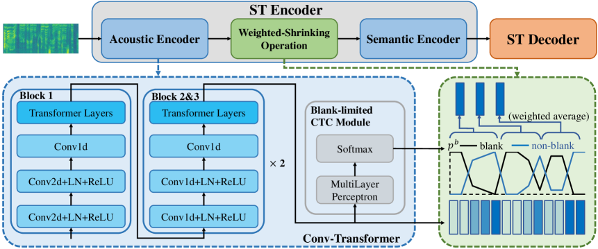
Our RealTranS follows the sequence-to-sequence architecture, which consists of an ST encoder and an ST decoder. The ST encoder is decoupled into three parts, an acoustic encoder, a weighted shrinking operation, and a semantic encoder, to gradually map speech inputs into semantic representation space of text. Figure 2 shows the architecture.
3.1 Problem Formulation
Speech translation corpora usually contain triples of speech, transcription and translation, denoted as . Specifically, is a sequence of speech features extracted from speech signals, e.g., filterbanks. and are the corresponding transcription in source language and translation in target language. , , and are the lengths of speech, transcription and translation, respectively, where usually and . A typical end-to-end model only makes use of and , while can be used as multi-task training for other objectives, like CTC loss.
3.2 Acoustic Encoder
Acoustic encoder mainly encodes speech features into a hidden space to learn acoustic knowledge. We apply Conv-Transformer Huang et al. (2020) to extract the desired features. It contains three blocks, each of which is composed of three convolution layers followed by unidirectional Transformer layers (see lower left in Figure 2) to prevent from leveraging future context in SST. Similar to Huang et al. (2020), we make the model aware of limited future frames with a look-ahead window in the convolution layers, to help improve acoustic modeling. At the same time, we gradually downsample the long speech features by setting the stride size to 2 in the second convolution layer in each block. In this way, the speech features are gradually reduced and approach the length of the corresponding text.
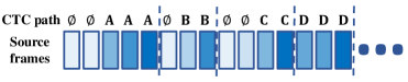
To predict the word boundaries111For ease of understanding, we use word boundaries here. Same methods can be applied to boundaries between phones, chars, subwords, etc., depending on the the granularity of the CTC loss units. We use subword units in our experiments. in the speech input and further improve the learned acoustic features, we adopt the Connectionist Temporal Classification (CTC) Graves et al. (2006) module on top of the acoustic encoder. This module contains a Multilayer Perceptron (MLP) followed by a Softmax operator. CTC predicts a path , where is the length of hidden states after the Conv-Transformer. And can be either a token in the source vocabulary or the blank symbol . CTC paths have the many-to-one mapping to output sequences by removing blank symbols and consecutively repeated labels, denoted as operation . Therefore, CTC loss is defined as follows:
| (1) |
where denotes all possible CTC paths that can be mapped to the transcription . With the CTC module, we can define a word boundary between two frames where the first frame has a non-blank label while the second frame has a different label from the first one. Figure 3 shows an example of word boundaries.
Due to the data scarcity problem in ST and CTC’s inherent characteristics Liu et al. (2018), the detected word boundaries are usually not accurate enough. The module will overly predict the occurrence of blank labels (as a kind of overfitting), resulting in a large gap between the number of detected boundaries and the number of tokens in transcription, especially when unidirectional Transformer is applied (see Table 3). To alleviate the problem, we add a blank penalty to encourage the module to produce non-blank labels. It is called blank-limited CTC loss and defined as follows:
| (2) |
where means the argmax results of CTC softmax outputs. controls the effect of blank penalty.
3.3 Weighted-Shrinking Operation
The length gap between acoustic features and the corresponding transcription and translation is still large after the gradual downsampling in Section 3.2. Inspired by previous studies Dong et al. (2020a); Liu et al. (2020), we adopt a shrinking operation to bridge the gap based on CTC predictions. Prior works usually either remove blank frames and then average repeated frames Dong et al. (2020a) or select a single representative frame Liu et al. (2020) in a detected segment (i.e., frames between two word boundaries). However, there might be useful information in the detected blank or repeated frames, especially when the boundary detection is not accurate enough (see Section 3.2).
We propose a weighted-shrinking mechanism to tackle the problem. We assume that the probability of a frame to be labeled as “blank” represents the confidence that the model “thinks” it is not important. Therefore, for the frames in one segment, their weights are decided by the probabilities to be blank labels. The representation of the segment will be the weighted average of the corresponding frames. The specific operation is shown as follows:
| (3) |
where denotes the probability of the frame to be blank, and represents the hidden state of the frame in our acoustic encoder. controls the temperature of the distribution (i.e., Softmax function). When , it means that we simply average the frames; and when it degenerates to the general shrinking mechanism where only the representative frames with the highest confidence are selected.
3.4 Semantic Encoder
The shrinking operation only bridges the length gap between speech and text, but the shrunk representations still lack semantic information. Therefore, we apply a semantic encoder on top of the shrunk representations Liu et al. (2020). It first applies a positional embedding layer, and then follows several Transformer layers (also unidirectional to mask future context), to extract semantic representations.
3.5 ST Decoder
A similar decoder as the basic Transformer architecture in NMT is adopted, where several Transformer decoder layers are stacked on top of target embeddings. To simulate simultaneous translation, we follow the prefix-to-prefix framework Ma et al. (2019) and mask certain future context in cross attention to ensure that the model predicts the current token based on only part of the input from the ST encoder. How much context the model can see depends on the simultaneous strategy that is applied. For example, a Wait-K Ma et al. (2019) based decoder predicts the -th token based on the first hidden states produced by the ST encoder.
Wait-K-Stride-N.
There is one drawback in the conventional Wait-K strategy – it cannot perform vanilla beam search while decoding except for the long-tail scenario Ma et al. (2019); Zheng et al. (2019c), though beam search has been proven very effective in improving translation quality. Based on the prefix-to-prefix framework and STATIC-RW strategy proposed in Dalvi et al. (2018), we propose the Wait-K-Stride-N strategy to allow using beam search for local reranking during simultaneous decoding. Similar to the Wait-K strategy, our strategy first reads input units (tokens in MT or segments in ST). Then, the model repeatedly performs write and read operations until the end of the sentence (see Figure 4). In this way, the translation latency is close to Wait-K, but we can perform beam search during the write operations. The objective with such a strategy is hence defined as follows:
| (4) |
where represents the target tokens before , is the length of the target sentence, and represents the first detected source segments.
3.6 Training Procedure
The total objective of our model will be the sum of the CTC part and the ST part:
| (5) |
where controls the influence of the CTC part.
To enhance the CTC quality, we also apply a pre-training procedure Stoian et al. (2020). We only use CTC loss to pre-train the acoustic encoder222We do not pre-train the decoder for simplicity though it might further improve our performance.. In this way, we can prevent the training waste Wang et al. (2020b), and focus on improving the alignment results, which are essential for shrinking operations (see Table 3). The whole model is then fine-tuned with the whole ST corpus.
4 Experimental Setup
4.1 Datasets
We conduct experiments on three publicly available datasets: Augmented LibriSpeech English-French (En–Fr) corpus Kocabiyikoglu et al. (2018), and MUST-C English-Spanish (En–Es) and English-German (En–De) corpus Di Gangi et al. (2019). All the datasets include source audios with the corresponding transcriptions in source language and translations in target language. For the Augmented Librispeech En–Fr corpus, we follow previous work Wang et al. (2020c) and use the 100-hour clean training set with aligned references and provided Google translations, resulting in double size of training pairs. For MUST-C datasets, We use the official data splits for train and development and tst-COMMON set for test. The statistics for these three datasets are listed in Table 1.
4.2 Experimental Settings
We use 80-dimensional log-mel filterbanks as acoustic features, which are calculated with 25ms window size and 10ms step size and normalized by utterance-level Cepstral Mean and Variance Normalization (CMVN). For transcriptions and translations, SentencePiece333https://github.com/google/sentencepiece Kudo and Richardson (2018) is used to generate subword vocabularies with the sizes of 4k and 8k respectively. We remove the punctuation in transcriptions.
| Corpus | Train | Dev | Test |
|---|---|---|---|
| En–Fr | 47,2712 (100h) | 1,071 (2.0h) | 2,048 (4.0h) |
| En–Es | 265,625 (496h) | 1,316 (2.5h) | 2,502 (4.0h) |
| En–De | 229,703 (400h) | 1,423 (2.5h) | 2,641 (4.0h) |
Our acoustic encoder follows the settings of the original Conv-Transformer Huang et al. (2020), except that the channel number in convolution layers and hidden size and head number in Transformer layers are half values of theirs. This means the output dimension of the acoustic encoder is 256. We use 6 Transformer layers in the semantic encoder and 4 in the ST decoder. The hyper-parameters (Eq. 2), (Eq. 3) and (Eq. 5) in our model are set to , and , respectively.
Our model is trained with 8 NVIDIA Tesla V100 GPUs, batched with an approximate 40000-frame features. We use Adam optimizer Kingma and Ba (2015) with a 0.002 learning rate and 10000 warm-up steps followed by the inverse square root scheduler. Dropout strategy is used with a rate of . We save checkpoints every epoch and average the last 10 checkpoints for evaluation with a beam size of . For simplicity, we use the same K and N values as those of training for inference. We implement our model based on Fairseq S2T444https://github.com/pytorch/fairseq/tree/master/examples/speech_to_text Wang et al. (2020a).
4.3 Evaluation Metrics
We apply SacreBLEU555https://github.com/mjpost/sacreBLEU for translation quality evaluation unless otherwise stated. For the metrics of latency, we adapt Average Proportion (AP) Cho and Esipova (2016) and Average Lagging (AL) Ma et al. (2019) to ST settings, following previous studies Ren et al. (2020); Ma et al. (2020a).
Average Proportion.
AP calculates the mean absolute latency cost by each target token, where we replace the steps of source tokens with the time spent. It can be calculated as follows:
| (6) |
where is the speech duration that has been listened when producing the target token .
Average Lagging.
AL evaluates the degree of that the user is out of sync with the speaker, in terms of the number of source tokens Ma et al. (2019). Following Ma et al. (2020a), we also extend it to the basis of time duration rather than source tokens, which is defined as follows:
| (7) |
where is the length of the reference translation, and denotes the index of the corresponding target token when our model has read the entire source speech. represents that the speech features are extracted every ms (decided by the step size in the feature extraction and downsampling rates in convolution layers), which will be 80ms in our model. What’s more, our Conv-Transformer module introduces a 140ms look-ahead window Huang et al. (2020), so we add 140 to the final AL scores to be fairly compared with other models.
5 Experimental Results
This section displays our experimental results. To explicitly show the performance trend of models in different scenarios, we use line charts to display most of the compared results. Their corresponding numeric results can be found in Appendix A.
5.1 Translation Quality vs. Latency
We first evaluate our RealTranS model with our Wait-K-Stride-N simultaneous strategy on the three datasets. We select three values 1, 2 and 3 for N to compare (it becomes conventional Wait-K when N1). The results are displayed in Figure 5.
Results show that RealTranS achieves higher BLEU scores as the K value increases, with sacrfice of translation delay, consistent with prior works Ren et al. (2020); Ma et al. (2020a).
Compared to the conventional Wait-K (N1), our model with N2 can achieve better BLEU scores under the same latency requirements, which demonstrates the effectiveness of our proposed Wait-K-Stride-N strategy. When N3, the latency becomes higher. And it only achieves similar gains in BLEU scores compared to N2 on MUST-C En–Es and En–De datasets. Therefore, we will use N2 as our simultaneous strategy in later experiments unless otherwise stated.
5.2 Comparison with SimulSpeech
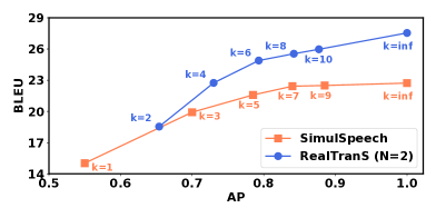
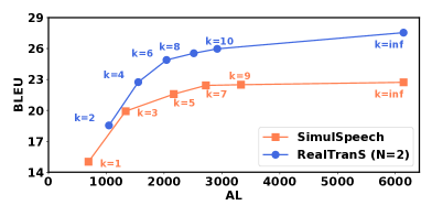
We compare with SimulSpeech Ren et al. (2020), the state-of-the-art end-to-end model for SST. Figure 6 shows the performance comparison on the MUST-C En-Es dataset (we report tokenized case-sensitive BLEU scores following their settings). Since they only report segment-based AL, we transfer it to our time-based AL proportionally based on the latency when Kinf.
We find that our RealTranS model outperforms SimulSpeech almost in all latency settings, with an average of about higher BLEU scores. Although SimulSpeech achieves relatively lower latency (e.g. less than 1000 ms AL when K1), the performance inevitably suffers. What’s more, SimulSpeech has leveraged multi-task learning and knowledge distillation to enhance their performance, which can be also applied to further improve the performance of our RealTranS model.
5.3 Comparison with Cascaded Model
We implement a cascaded model to compare with RealTranS under the same latency. Specifically, we combine our acoustic encoder (Section 3.2) and a Transformer decoder as our ASR model and use the conventional Transformer encoder-decoder architecture as our NMT model. Their configuration is similar to RealTranS (e.g. the same hidden dimension and the same number of Transformer layers). And we train the ASR and NMT model with the same corpus. The conventional Wait-K strategy is used in the ASR model since the alignment between speech and transcription is monotonic, while Wait-K-Stride-N is applied in the NMT model. Since several combinations of the ASR and NMT models may be under the same latency, we report the best BLEU score among them.
| Model | K2 | K4 | K6 | K8 | K10 | Kinf |
|---|---|---|---|---|---|---|
| Cascaded | 14.92 | 19.22 | 22.11 | 23.33 | 24.47 | 26.79 |
| RealTranS | 18.45 | 22.65 | 24.79 | 25.41 | 25.82 | 27.40 |
Table 2 shows the comparison results on MUST-C En–Es dataset. We have the following observations: 1) our RealTranS model outperforms the cascaded model in all latency settings, which demonstrates the superiority of RealTranS. 2) The improvement over the cascaded model becomes larger when the value of K is smaller. This observation is consistent with Ren et al. (2020). We attribute this to the advantage of end-to-end models over cascaded models, where the impact of error propagation in cascaded models may be amplified when the latency is low.
5.4 Effects of Blank Penalty and Weighted Shrinking Operation
In this subsection, we examine the effects of our proposed methods, including blank penalty (Eq. 2) and weighted-shrinking operation (Eq. 3).
Blank Penalty.
We propose a blank penalty to alleviate the inaccuracy of alignments between speech features and transcriptions when applying unidirectional encoders for SST (Section 3.2). To examine the effect, we evaluate the shrinking quality, i.e., the differences between the length of representations after the shrinking operation and that of the ground-truth transcription, on MUST-C En–Es dataset, and display the statistics in Table 3. We can see that the performance, as well as the shrinking quality, drops when removing CTC pre-training. It further decreases when removing the blank penalty, which shows its effectiveness. Also, we can see that the performance loss partly comes from using unidirectional encoders rather than bidirectional for simultaneous purposes (the th row), which can be compensated by the blank penalty.
| Model | Diff2 | Diff4 | Diff6 | BLEU |
|---|---|---|---|---|
| Full Model | 52% | 74% | 85% | 27.40 |
| - CTC PT | 48% | 70% | 82% | 26.63 |
| - BP | 35% | 53% | 67% | 25.76 |
| + Bi-Enc | 42% | 59% | 72% | 26.58 |
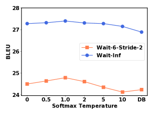
Weighted-Shrinking.
To validate our weighted-shrinking operation, we first investigate the effects of various values for the shrinking temperature in Eq. 3 and display the results in Figure 7(a). The results show that our weighted-shrinking mechanism () performs better than both simply averaging all the frames () and dropping blank frames (“DB”).
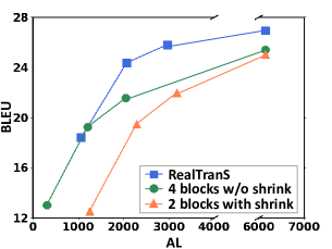
We also try to replace our weighted-shrinking module with another Conv-Transformer block (see Section 3.2), resulting in a model with 240ms downsample rate in total (denoted as “4 blocks w/o shrink”). Figure 7(b) shows comparison results, together with a model with only 2 blocks (40ms downsample rate, denoted as “2 blocks with shrink”). We can find that downsampling only with convolution layers performs worse than RealTranS, while less downsample rate also affects the performance. This implies that there is an upper-bound for downsampling with only convolution layers while maintaining performance, and our weighted-shrinking operation can be used as an addition to further improve the performance.
5.5 Ablation Study
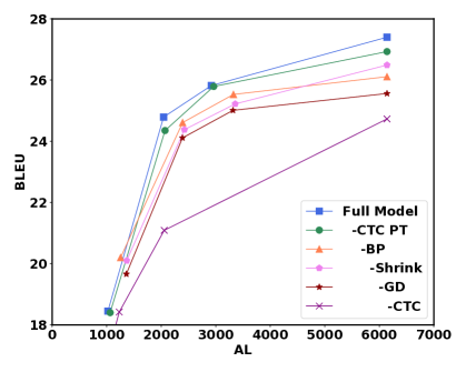
We evaluate the contributions of different modules in RealTranS. Each module is evaluated in four kinds of latency settings: Wait-2-Stride-2, Wait-6-Stride-2, Wait-10-Stride-2, and also Wait-Inf (full sentence translation). The results are shown in Figure 8, where “-CTC PT” means we do not pre-train the encoder with CTC loss and “-BP” indicates we further remove the blank penalty. “-shrink” means removing the weighted-shrinking operation and the semantic encoder, while “-GD” denotes disabling the gradual downsampling by moving the Transformer layers in block 1 & 2 to block 3 (see Figure 2) to perform downsampling at the beginning layers of the acoustic encoder. Finally, “-CTC” indicates that CTC objective is removed.
Figure 8 shows that all modules play a role in RealTranS. Specifically, we have the following observations: 1) The CTC module is important for improving translation quality, and it can be further improved by pre-training. 2) The blank penalty is useful in reducing latency while maintaining translation quality. 3) The blank penalty is essential for the shrinking operation since on full sentence translation the shrinking operation degrades the performance without the blank penalty (“-BP” vs “-Shrink”). 4) Gradual downsampling also contributes to the performance, because directly downsampling to a large rate may make it difficult to learn acoustic features.
5.6 Comparison in Full Sentence Translation
| Dataset | Method | BLEU |
| En-Fr | Transformer+KD Liu et al. (2019) | 17.02 |
| TCEN-LSTM Wang et al. (2020b) | 17.05 | |
| Curriculum PT Wang et al. (2020c) | 17.66 | |
| LUT Dong et al. (2020b) | 17.75 | |
| STAST Liu et al. (2020) | 17.81 | |
| COSTT Dong et al. (2020a) | 17.83 | |
| Transformer+AFS Zhang et al. (2020) | 18.56⋆ | |
| RealTranS (ours) | 18.97 | |
| 18.30⋆ | ||
| En-De | Transformer+MAM Chen et al. (2020) | 21.87⋆ |
| Transformer+ML Indurthi et al. (2019) | 22.11⋆ | |
| Transformer+AFS Zhang et al. (2020) | 22.38⋆ | |
| Fairseq S2T Wang et al. (2020a) | 22.70⋆ | |
| Espnet ST Inaguma et al. (2020) | 22.91⋆ | |
| STAST Liu et al. (2020) | 23.06 | |
| RealTranS (ours) | 23.53 | |
| 22.99⋆ |
Although focusing on SST, RealTranS can also be applied in full sentence ST. For fair comparison, we replace the unidirectional Transformer layers in RealTranS with bidirectional ones and report both case-insensitive and case-sensitive BLEU scores following prior works. Table 4 displays the BLEU scores compared with existing methods (we only compare with end-to-end models trained with the same data for fair comparison) on Augmented LibriSpeech En–Fr and MUST-C En–De dataset. RealTranS yields competitive (En–Fr) or even better (En–De) results, even though most of these prior methods depend on some extra techniques like pre-training decoders or using SpecAugment Park et al. (2019). This validates the superiority of our proposed architecture.
6 Conclusion
This work proposes a new end-to-end model RealTranS and a new strategy Wait-K-Stride-N for SST. RealTranS gradually bridges the modality gap between speech and text, and achieves new state-of-the-art results for SST. Empirical studies have shown the proposed blank penalty for CTC loss helps on the alignment with transcription, which reduces latency while maintaining translation quality. Our weighted-shrinking operation, as well as Wait-K-Stride-N simultaneous strategy, further improves the performance. We also compare RealTranS with other methods for full sentence translation, where RealTranS still exhibits competitive results, showing its superiority.
References
- Anastasopoulos and Chiang (2018) Antonios Anastasopoulos and David Chiang. 2018. Tied multitask learning for neural speech translation. In Proceedings of the 2018 Conference of the North American Chapter of the Association for Computational Linguistics: Human Language Technologies, Volume 1 (Long Papers), pages 82–91, New Orleans, Louisiana. Association for Computational Linguistics.
- Arivazhagan et al. (2019) Naveen Arivazhagan, Colin Cherry, Wolfgang Macherey, Chung-Cheng Chiu, Semih Yavuz, Ruoming Pang, Wei Li, and Colin Raffel. 2019. Monotonic infinite lookback attention for simultaneous machine translation. In Proceedings of the 57th Annual Meeting of the Association for Computational Linguistics, pages 1313–1323, Florence, Italy. Association for Computational Linguistics.
- Bahar et al. (2021) Parnia Bahar, Tobias Bieschke, Ralf Schlüter, and Hermann Ney. 2021. Tight integrated end-to-end training for cascaded speech translation. In IEEE Spoken Language Technology Workshop, SLT 2021, Shenzhen, China, January 19-22, 2021, pages 950–957. IEEE.
- Bahar et al. (2019) Parnia Bahar, Albert Zeyer, Ralf Schlüter, and Hermann Ney. 2019. On using specaugment for end-to-end speech translation. CoRR, abs/1911.08876.
- Bansal et al. (2018) Sameer Bansal, Herman Kamper, Karen Livescu, Adam Lopez, and Sharon Goldwater. 2018. Low-resource speech-to-text translation. In Interspeech 2018, 19th Annual Conference of the International Speech Communication Association, Hyderabad, India, 2-6 September 2018, pages 1298–1302. ISCA.
- Bansal et al. (2019) Sameer Bansal, Herman Kamper, Karen Livescu, Adam Lopez, and Sharon Goldwater. 2019. Pre-training on high-resource speech recognition improves low-resource speech-to-text translation. In Proceedings of the 2019 Conference of the North American Chapter of the Association for Computational Linguistics: Human Language Technologies, Volume 1 (Long and Short Papers), pages 58–68, Minneapolis, Minnesota. Association for Computational Linguistics.
- Berard et al. (2018) Alexandre Berard, Laurent Besacier, Ali Can Kocabiyikoglu, and Olivier Pietquin. 2018. End-to-end automatic speech translation of audiobooks. In 2018 IEEE International Conference on Acoustics, Speech and Signal Processing, ICASSP 2018, Calgary, AB, Canada, April 15-20, 2018, pages 6224–6228. IEEE.
- Berard et al. (2016) Alexandre Berard, Olivier Pietquin, Christophe Servan, and Laurent Besacier. 2016. Listen and translate: A proof of concept for end-to-end speech-to-text translation. CoRR, abs/1612.01744.
- Chen et al. (2020) Junkun Chen, Mingbo Ma, Renjie Zheng, and Liang Huang. 2020. MAM: masked acoustic modeling for end-to-end speech-to-text translation. CoRR, abs/2010.11445.
- Cho and Esipova (2016) Kyunghyun Cho and Masha Esipova. 2016. Can neural machine translation do simultaneous translation? CoRR, abs/1606.02012.
- Dalvi et al. (2018) Fahim Dalvi, Nadir Durrani, Hassan Sajjad, and Stephan Vogel. 2018. Incremental decoding and training methods for simultaneous translation in neural machine translation. In Proceedings of the 2018 Conference of the North American Chapter of the Association for Computational Linguistics: Human Language Technologies, Volume 2 (Short Papers), pages 493–499, New Orleans, Louisiana. Association for Computational Linguistics.
- Di Gangi et al. (2019) Mattia A. Di Gangi, Roldano Cattoni, Luisa Bentivogli, Matteo Negri, and Marco Turchi. 2019. MuST-C: a Multilingual Speech Translation Corpus. In Proceedings of the 2019 Conference of the North American Chapter of the Association for Computational Linguistics: Human Language Technologies, Volume 1 (Long and Short Papers), pages 2012–2017, Minneapolis, Minnesota. Association for Computational Linguistics.
- Dong et al. (2020a) Qianqian Dong, Mingxuan Wang, Hao Zhou, Shuang Xu, Bo Xu, and Lei Li. 2020a. Consecutive decoding for speech-to-text translation. CoRR, abs/2009.09737.
- Dong et al. (2020b) Qianqian Dong, Mingxuan Wang, Hao Zhou, Shuang Xu, Bo Xu, and Lei Li. 2020b. Listen, understand and translate: Triple supervision decouples end-to-end speech-to-text translation. CoRR, abs/2009.09704.
- Fügen et al. (2007) Christian Fügen, Alex Waibel, and Muntsin Kolss. 2007. Simultaneous translation of lectures and speeches. Mach. Transl., 21(4):209–252.
- Gangi et al. (2019) Mattia Antonino Di Gangi, Matteo Negri, and Marco Turchi. 2019. Adapting transformer to end-to-end spoken language translation. In Interspeech 2019, 20th Annual Conference of the International Speech Communication Association, Graz, Austria, 15-19 September 2019, pages 1133–1137. ISCA.
- Graves et al. (2006) Alex Graves, Santiago Fernández, Faustino J. Gomez, and Jürgen Schmidhuber. 2006. Connectionist temporal classification: labelling unsegmented sequence data with recurrent neural networks. In Machine Learning, Proceedings of the Twenty-Third International Conference (ICML 2006), Pittsburgh, Pennsylvania, USA, June 25-29, 2006, volume 148 of ACM International Conference Proceeding Series, pages 369–376. ACM.
- Gu et al. (2017) Jiatao Gu, Graham Neubig, Kyunghyun Cho, and Victor O.K. Li. 2017. Learning to translate in real-time with neural machine translation. In Proceedings of the 15th Conference of the European Chapter of the Association for Computational Linguistics: Volume 1, Long Papers, pages 1053–1062, Valencia, Spain. Association for Computational Linguistics.
- Huang et al. (2020) Wenyong Huang, Wenchao Hu, Yu Ting Yeung, and Xiao Chen. 2020. Conv-transformer transducer: Low latency, low frame rate, streamable end-to-end speech recognition. In Interspeech 2020, 21st Annual Conference of the International Speech Communication Association, Virtual Event, Shanghai, China, 25-29 October 2020, pages 5001–5005. ISCA.
- Inaguma et al. (2020) Hirofumi Inaguma, Shun Kiyono, Kevin Duh, Shigeki Karita, Nelson Yalta, Tomoki Hayashi, and Shinji Watanabe. 2020. ESPnet-ST: All-in-one speech translation toolkit. In Proceedings of the 58th Annual Meeting of the Association for Computational Linguistics: System Demonstrations, pages 302–311, Online. Association for Computational Linguistics.
- Indurthi et al. (2019) Sathish Reddy Indurthi, Houjeung Han, Nikhil Kumar Lakumarapu, Beomseok Lee, Insoo Chung, Sangha Kim, and Chanwoo Kim. 2019. Data efficient direct speech-to-text translation with modality agnostic meta-learning. CoRR, abs/1911.04283.
- Iranzo-Sánchez et al. (2020) Javier Iranzo-Sánchez, Adrià Giménez Pastor, Joan Albert Silvestre-Cerdà, Pau Baquero-Arnal, Jorge Civera Saiz, and Alfons Juan. 2020. Direct segmentation models for streaming speech translation. In Proceedings of the 2020 Conference on Empirical Methods in Natural Language Processing (EMNLP), pages 2599–2611, Online. Association for Computational Linguistics.
- Jia et al. (2019) Ye Jia, Melvin Johnson, Wolfgang Macherey, Ron J. Weiss, Yuan Cao, Chung-Cheng Chiu, Naveen Ari, Stella Laurenzo, and Yonghui Wu. 2019. Leveraging weakly supervised data to improve end-to-end speech-to-text translation. In IEEE International Conference on Acoustics, Speech and Signal Processing, ICASSP 2019, Brighton, United Kingdom, May 12-17, 2019, pages 7180–7184. IEEE.
- Kingma and Ba (2015) Diederik P. Kingma and Jimmy Ba. 2015. Adam: A method for stochastic optimization. In 3rd International Conference on Learning Representations, ICLR 2015, San Diego, CA, USA, May 7-9, 2015, Conference Track Proceedings.
- Kocabiyikoglu et al. (2018) Ali Can Kocabiyikoglu, Laurent Besacier, and Olivier Kraif. 2018. Augmenting librispeech with french translations: A multimodal corpus for direct speech translation evaluation. In Proceedings of the Eleventh International Conference on Language Resources and Evaluation, LREC 2018, Miyazaki, Japan, May 7-12, 2018. European Language Resources Association (ELRA).
- Kudo and Richardson (2018) Taku Kudo and John Richardson. 2018. SentencePiece: A simple and language independent subword tokenizer and detokenizer for neural text processing. In Proceedings of the 2018 Conference on Empirical Methods in Natural Language Processing: System Demonstrations, pages 66–71, Brussels, Belgium. Association for Computational Linguistics.
- Liu et al. (2018) Hu Liu, Sheng Jin, and Changshui Zhang. 2018. Connectionist temporal classification with maximum entropy regularization. In Advances in Neural Information Processing Systems 31: Annual Conference on Neural Information Processing Systems 2018, NeurIPS 2018, December 3-8, 2018, Montréal, Canada, pages 839–849.
- Liu et al. (2019) Yuchen Liu, Hao Xiong, Jiajun Zhang, Zhongjun He, Hua Wu, Haifeng Wang, and Chengqing Zong. 2019. End-to-end speech translation with knowledge distillation. In Interspeech 2019, 20th Annual Conference of the International Speech Communication Association, Graz, Austria, 15-19 September 2019, pages 1128–1132. ISCA.
- Liu et al. (2020) Yuchen Liu, Junnan Zhu, Jiajun Zhang, and Chengqing Zong. 2020. Bridging the modality gap for speech-to-text translation. CoRR, abs/2010.14920.
- Ma et al. (2019) Mingbo Ma, Liang Huang, Hao Xiong, Renjie Zheng, Kaibo Liu, Baigong Zheng, Chuanqiang Zhang, Zhongjun He, Hairong Liu, Xing Li, Hua Wu, and Haifeng Wang. 2019. STACL: Simultaneous translation with implicit anticipation and controllable latency using prefix-to-prefix framework. In Proceedings of the 57th Annual Meeting of the Association for Computational Linguistics, pages 3025–3036, Florence, Italy. Association for Computational Linguistics.
- Ma et al. (2020a) Xutai Ma, Juan Pino, and Philipp Koehn. 2020a. SimulMT to SimulST: Adapting simultaneous text translation to end-to-end simultaneous speech translation. In Proceedings of the 1st Conference of the Asia-Pacific Chapter of the Association for Computational Linguistics and the 10th International Joint Conference on Natural Language Processing, pages 582–587, Suzhou, China. Association for Computational Linguistics.
- Ma et al. (2020b) Xutai Ma, Yongqiang Wang, Mohammad Javad Dousti, Philipp Koehn, and Juan Pino. 2020b. Streaming simultaneous speech translation with augmented memory transformer. CoRR, abs/2011.00033.
- Mathias and Byrne (2006) Lambert Mathias and William Byrne. 2006. Statistical phrase-based speech translation. In 2006 IEEE International Conference on Acoustics Speech and Signal Processing, ICASSP 2006, Toulouse, France, May 14-19, 2006, pages 561–564. IEEE.
- Ney (1999) Hermann Ney. 1999. Speech translation: coupling of recognition and translation. In Proceedings of the 1999 IEEE International Conference on Acoustics, Speech, and Signal Processing, ICASSP ’99, Phoenix, Arizona, USA, March 15-19, 1999, pages 517–520. IEEE Computer Society.
- Oda et al. (2014) Yusuke Oda, Graham Neubig, Sakriani Sakti, Tomoki Toda, and Satoshi Nakamura. 2014. Optimizing segmentation strategies for simultaneous speech translation. In Proceedings of the 52nd Annual Meeting of the Association for Computational Linguistics (Volume 2: Short Papers), pages 551–556, Baltimore, Maryland. Association for Computational Linguistics.
- Park et al. (2019) Daniel S. Park, William Chan, Yu Zhang, Chung-Cheng Chiu, Barret Zoph, Ekin D. Cubuk, and Quoc V. Le. 2019. Specaugment: A simple data augmentation method for automatic speech recognition. In Interspeech 2019, 20th Annual Conference of the International Speech Communication Association, Graz, Austria, 15-19 September 2019, pages 2613–2617. ISCA.
- Ren et al. (2020) Yi Ren, Jinglin Liu, Xu Tan, Chen Zhang, Tao Qin, Zhou Zhao, and Tie-Yan Liu. 2020. SimulSpeech: End-to-end simultaneous speech to text translation. In Proceedings of the 58th Annual Meeting of the Association for Computational Linguistics, pages 3787–3796, Online. Association for Computational Linguistics.
- Salesky and Black (2020) Elizabeth Salesky and Alan W Black. 2020. Phone features improve speech translation. In Proceedings of the 58th Annual Meeting of the Association for Computational Linguistics, pages 2388–2397, Online. Association for Computational Linguistics.
- Sperber et al. (2017) Matthias Sperber, Graham Neubig, Jan Niehues, and Alex Waibel. 2017. Neural lattice-to-sequence models for uncertain inputs. In Proceedings of the 2017 Conference on Empirical Methods in Natural Language Processing, pages 1380–1389, Copenhagen, Denmark. Association for Computational Linguistics.
- Stoian et al. (2020) Mihaela C. Stoian, Sameer Bansal, and Sharon Goldwater. 2020. Analyzing ASR pretraining for low-resource speech-to-text translation. In 2020 IEEE International Conference on Acoustics, Speech and Signal Processing, ICASSP 2020, Barcelona, Spain, May 4-8, 2020, pages 7909–7913. IEEE.
- Wang et al. (2020a) Changhan Wang, Yun Tang, Xutai Ma, Anne Wu, Dmytro Okhonko, and Juan Pino. 2020a. Fairseq S2T: Fast speech-to-text modeling with fairseq. In Proceedings of the 1st Conference of the Asia-Pacific Chapter of the Association for Computational Linguistics and the 10th International Joint Conference on Natural Language Processing: System Demonstrations, pages 33–39, Suzhou, China. Association for Computational Linguistics.
- Wang et al. (2020b) Chengyi Wang, Yu Wu, Shujie Liu, Zhenglu Yang, and Ming Zhou. 2020b. Bridging the gap between pre-training and fine-tuning for end-to-end speech translation. In The Thirty-Fourth AAAI Conference on Artificial Intelligence, AAAI 2020, The Thirty-Second Innovative Applications of Artificial Intelligence Conference, IAAI 2020, The Tenth AAAI Symposium on Educational Advances in Artificial Intelligence, EAAI 2020, New York, NY, USA, February 7-12, 2020, pages 9161–9168. AAAI Press.
- Wang et al. (2020c) Chengyi Wang, Yu Wu, Shujie Liu, Ming Zhou, and Zhenglu Yang. 2020c. Curriculum pre-training for end-to-end speech translation. In Proceedings of the 58th Annual Meeting of the Association for Computational Linguistics, pages 3728–3738, Online. Association for Computational Linguistics.
- Weiss et al. (2017) Ron J. Weiss, Jan Chorowski, Navdeep Jaitly, Yonghui Wu, and Zhifeng Chen. 2017. Sequence-to-sequence models can directly transcribe foreign speech. CoRR, abs/1703.08581.
- Zhang et al. (2020) Biao Zhang, Ivan Titov, Barry Haddow, and Rico Sennrich. 2020. Adaptive feature selection for end-to-end speech translation. In Findings of the Association for Computational Linguistics: EMNLP 2020, pages 2533–2544, Online. Association for Computational Linguistics.
- Zheng et al. (2020) Baigong Zheng, Kaibo Liu, Renjie Zheng, Mingbo Ma, Hairong Liu, and Liang Huang. 2020. Simultaneous translation policies: From fixed to adaptive. In Proceedings of the 58th Annual Meeting of the Association for Computational Linguistics, pages 2847–2853, Online. Association for Computational Linguistics.
- Zheng et al. (2019a) Baigong Zheng, Renjie Zheng, Mingbo Ma, and Liang Huang. 2019a. Simpler and faster learning of adaptive policies for simultaneous translation. In Proceedings of the 2019 Conference on Empirical Methods in Natural Language Processing and the 9th International Joint Conference on Natural Language Processing (EMNLP-IJCNLP), pages 1349–1354, Hong Kong, China. Association for Computational Linguistics.
- Zheng et al. (2019b) Baigong Zheng, Renjie Zheng, Mingbo Ma, and Liang Huang. 2019b. Simultaneous translation with flexible policy via restricted imitation learning. In Proceedings of the 57th Annual Meeting of the Association for Computational Linguistics, pages 5816–5822, Florence, Italy. Association for Computational Linguistics.
- Zheng et al. (2019c) Renjie Zheng, Mingbo Ma, Baigong Zheng, and Liang Huang. 2019c. Speculative beam search for simultaneous translation. In Proceedings of the 2019 Conference on Empirical Methods in Natural Language Processing and the 9th International Joint Conference on Natural Language Processing (EMNLP-IJCNLP), pages 1395–1402, Hong Kong, China. Association for Computational Linguistics.
Appendix
Appendix A Numeric Results for the Figures
| N Value | K=N | K=N+2 | K=N+4 | K=N+6 | K=N+8 | |||||
|---|---|---|---|---|---|---|---|---|---|---|
| BLEU | AL | BLEU | AL | BLEU | AL | BLEU | AL | BLEU | AL | |
| N=1 | 12.72 | 1710 | 15.04 | 2263 | 15.9 | 2748 | 16.6 | 3160 | 16.71 | 3572 |
| N=2 | 13.51 | 1792 | 15.63 | 2378 | 16.37 | 2856 | 16.87 | 3291 | 17.18 | 3669 |
| N=3 | 14.81 | 2004 | 16.13 | 2519 | 16.84 | 2962 | 17.04 | 3383 | 17.26 | 3746 |
| N Value | K=N | K=N+2 | K=N+4 | K=N+6 | K=N+8 | |||||
|---|---|---|---|---|---|---|---|---|---|---|
| BLEU | AL | BLEU | AL | BLEU | AL | BLEU | AL | BLEU | AL | |
| N=1 | 16.32 | 916 | 21.23 | 1426 | 23.53 | 1924 | 25.06 | 2399 | 25.45 | 2830 |
| N=2 | 18.45 | 1047 | 22.65 | 1554 | 24.79 | 2043 | 25.41 | 2514 | 25.82 | 2920 |
| N=3 | 21.74 | 1445 | 24.26 | 1968 | 25.11 | 2461 | 25.29 | 2944 | 25.78 | 3356 |
| N Value | K=N | K=N+2 | K=N+4 | K=N+6 | K=N+8 | |||||
|---|---|---|---|---|---|---|---|---|---|---|
| BLEU | AL | BLEU | AL | BLEU | AL | BLEU | AL | BLEU | AL | |
| N=1 | 13.22 | 1100 | 16.65 | 1582 | 18.67 | 2059 | 19.66 | 2508 | 19.78 | 2913 |
| N=2 | 15.74 | 1233 | 18.12 | 1709 | 19.02 | 2169 | 20.06 | 2607 | 20.09 | 3005 |
| N=3 | 16.54 | 1355 | 18.49 | 1838 | 19.84 | 2290 | 20.05 | 2720 | 20.41 | 3106 |
| Model | K=N | K=N+2 | K=N+4 | K=N+6 | K=N+8 | K=inf | ||||||
|---|---|---|---|---|---|---|---|---|---|---|---|---|
| BLEU | AP | BLEU | AP | BLEU | AP | BLEU | AP | BLEU | AP | BLEU | AP | |
| SimulSpeech | 15.02 | 0.550 | 19.92 | 0.700 | 21.58 | 0.785 | 22.42 | 0.840 | 22.49 | 0.885 | 22.72 | 1.0 |
| RealTranS(N=2) | 18.54 | 0.654 | 22.74 | 0.730 | 24.89 | 0.793 | 25.54 | 0.842 | 25.97 | 0.877 | 27.54 | 1.0 |
| Model | K=N | K=N+2 | K=N+4 | K=N+6 | K=N+8 | K=inf | ||||||
|---|---|---|---|---|---|---|---|---|---|---|---|---|
| BLEU | AL | BLEU | AL | BLEU | AL | BLEU | AL | BLEU | AL | BLEU | AL | |
| SimulSpeech | 15.02 | 694 | 19.92 | 1336 | 21.58 | 2169 | 22.42 | 2724 | 22.49 | 3331 | 22.72 | 6141 |
| RealTranS(N=2) | 18.54 | 1047 | 22.74 | 1554 | 24.89 | 2043 | 25.54 | 2514 | 25.97 | 2920 | 27.54 | 6141 |
| Model | =0 | =0.5 | =1.0 | =2.0 | =5.0 | =10 | DB |
|---|---|---|---|---|---|---|---|
| Wait-6-Stride-2 | 24.50 | 24.64 | 24.79 | 24.61 | 24.35 | 24.13 | 24.24 |
| Wait-Inf | 27.28 | 27.32 | 27.40 | 27.31 | 27.28 | 27.15 | 26.89 |
| Model | K=2 | K=6 | K=10 | K=inf | ||||
|---|---|---|---|---|---|---|---|---|
| BLEU | AL | BLEU | AL | BLEU | AL | BLEU | AL | |
| RealTranS | 18.40 | 1064 | 24.35 | 2070 | 25.79 | 2963 | 26.93 | 6141 |
| 4 blocks w/o shrink | 13.03 | 307 | 19.25 | 1207 | 21.55 | 2051 | 25.38 | 6141 |
| 2 blocks with shrink | 12.53 | 1247 | 19.48 | 2286 | 21.97 | 3175 | 25.04 | 6141 |
| Model | K=2 | K=6 | K=10 | K=inf | ||||
|---|---|---|---|---|---|---|---|---|
| BLEU | AL | BLEU | AL | BLEU | AL | BLEU | AL | |
| Full Model | 18.45 | 1023 | 24.79 | 2043 | 25.82 | 2920 | 27.40 | 6141 |
| -CTC PT | 18.40 | 1064 | 24.35 | 2070 | 25.79 | 2963 | 26.93 | 6141 |
| -BP | 20.20 | 1255 | 24.61 | 2393 | 25.53 | 3325 | 26.11 | 6141 |
| -Shrink | 20.10 | 1368 | 24.38 | 2426 | 25.22 | 3357 | 26.49 | 6141 |
| -GD | 19.66 | 1360 | 24.11 | 2390 | 25.01 | 3316 | 25.56 | 6141 |
| -CTC | 12.48 | 342 | 18.42 | 1230 | 21.09 | 2055 | 24.73 | 6141 |