Temporal Averaging LSTM-based Channel Estimation Scheme for IEEE 802.11p Standard

Abstract

In vehicular communications, reliable channel estimation is critical for the system performance due to the doubly-dispersive nature of vehicular channels. IEEE 802.11p standard allocates insufficient pilots for accurate channel tracking. Consequently, conventional IEEE 802.11p estimators suffer from a considerable performance degradation, especially in high mobility scenarios. Recently, deep learning (DL) techniques have been employed for IEEE 802.11p channel estimation. Nevertheless, these methods suffer either from performance degradation in very high mobility scenarios or from large computational complexity. In this paper, these limitations are solved using a long short term memory (LSTM)-based estimation. The proposed estimator employs an LSTM unit to estimate the channel, followed by temporal averaging (TA) processing as a noise alleviation technique. Moreover, the noise mitigation ratio is determined analytically, thus validating the TA processing ability in improving the overall performance. Simulation results reveal the performance superiority of the proposed schemes compared to the recently proposed DL-based estimators, while recording a significant reduction in the computational complexity.

I Introduction

Vehicular communication technologies [1] describe a set of communication models that can be employed by vehicles in different application contexts, resulting in a well organized network infrastructure. The main motivation behind such technologies is to facilitate several future smart city applications including road safety and autonomous driving.

In general, wireless communications in vehicular environment encounter a critical reliability challenge due to the doubly selective nature of the vehicular channel that varies rapidly especially in high mobility scenarios. Moreover, a precisely-estimated channel is critical for the equalization, demodulation, and decoding operations performed at the receiver. Therefore, robust and accurate channel estimation plays a crucial role in determining the overall system performance. IEEE 802.11p standard is an international standard that defines vehicular communications specifications. However, IEEE 802.11p standard is based initially on the IEEE 802.11a standard that was proposed for indoor environments, where an insufficient number of pilots is allocated for channel estimation. As a result, IEEE 802.11p conventional estimators are based on the data-pilot aided (DPA) estimation, where the demapped data subcarriers, besides pilot subcarriers are employed in the channel estimation. In order to improve the DPA estimation performance, spectral temporal averaging (STA) estimator [2] applies averaging in both the time and the frequency domains as post processing operations to the DPA estimated channel. STA estimator performs well in low signal-to-noise ratio (SNR) region, however it suffers from a significant performance degradation in high SNR region especially in high mobility vehicular scenarios. The time domain reliable test frequency domain interpolation (TRFI) [3] estimator assumes high correlation between successive symbols, thus it employs frequency domain interpolation to improve the DPA performance. TRFI estimator outperforms the STA estimator in high SNR region, however, these conventional estimators suffer from a considerable performance degradation in high mobility scenarios.

Recently, the rapid advancements in DL and their successful applications in several domains, have sparked significant interest to adopt DL techniques for wireless communication applications including channel estimation. DL techniques are characterized by robustness, low-complexity, and good generalization ability making their integration into communication systems beneficial. Motivated by these advantages, DL algorithms have been used for IEEE 802.11p channel estimator, where the authors in [4] and [5] employ deep neural networks (DNN) as a post processing unit after the STA and TRFI conventional estimators respectively. The simulation results have showed that STA-DNN and TRFI-DNN are able to significantly improve the performance, however, they suffer from an error floor in high mobility scenarios. Another different DL-based approach has been proposed in [6], where LSTM unit followed by DNN network are employed as a pre-processing modules for channel estimation and noise error compensation. After that, DPA estimation is applied using the DNN output. This LSTM-DNN-DPA estimator, outperforms the recently proposed STA-DNN and TRFI-DNN estimators, but it suffers from a considerable computational complexity due to the employment of two consecutive DL networks.

In order to overcome the high complexity of the LSTM-DNN-DPA estimator, while improving the bit error rate (BER) and normalized mean-squared error (NMSE) performances, in this paper we propose an LSTM-based estimator, where the channel is estimated using an LSTM unit only. After that, DPA estimation is applied using the LSTM estimated channel. Finally, unlike the LSTM-DNN-DPA estimator where DNN network is used for noise elimination, in the proposed estimator, TA processing is employed as a noise alleviation technique where the noise alleviation ratio is calculated analytically. We also provide a detailed computational complexity analysis and make a comparison between the recent related work on LSTM-DNN-DPA estimator and our proposed LSTM-DPA-TA estimator.

The remainder of this paper is organized as follows: in Section II, the system model followed by the recently proposed state-of-the-art (SoA) DL-based IEEE 802.11p estimators are provided. The proposed LSTM-DPA-TA, as well as the TA processing analytical derivation, are described in Section III. In Section IV, simulation results and computational complexity analysis are presented where the performance of the proposed scheme is evaluated in terms of BER. Finally, the paper is concluded in Section V.

II SoA DNN-Based Channel Estimators

II-A System Model

IEEE 802.11p standard employs orthogonal frequency-division multiplexing (OFDM) transmission scheme with ${K=64}$ total subcarriers. ${K_{\text{on}}=52}$ active subcarriers are used, and they are divided into ${K_{\text{d}}=48}$ data subcarriers and ${K_{\text{p}}=4}$ pilot subcarriers. The remaining ${K_{\text{n}}=12}$ subcarriers are used as a guard band. Moreover, IEEE 802.11p frame structure consists mainly of three parts. The first part contains the preamble that is used at the receiver for signal detection, timing synchronization, and channel estimation. Second, the signal field carries the transmission parameters like the employed code rate, modulation order, and frame length. Finally, we have the OFDM data symbols. A detailed discussion of the IEEE 802.p standard and all its features are presented in [7].

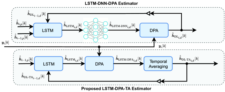
Figure 1: LSTM-based IEEE 802.11p channel estimators block diagram.

In this paper, we assume perfect synchronization at the receiver, and we omit the signal field for simplicity. Therefore, we consider only the two long training symbols followed by $I$ OFDM data symbols within each transmitted frame. The received OFDM symbol can be expressed as:

$$\small\tilde{\bm{y}}_{i}[k]=\left\{\begin{array}[]{ll}\tilde{\bm{h}}_{i,d}[k]\tilde{\bm{x}}_{i,d}[k]+\tilde{\bm{v}}_{i,d}[k],&\quad k\in{\mathcal{K}}_{\text{d}}\\ \tilde{\bm{h}}_{i,p}[k]\tilde{\bm{x}}_{i,p}[k]+\tilde{\bm{v}}_{i,p}[k],&\quad k\in{\mathcal{K}}_{\text{p}}\\ \end{array}\right.,$$ (1)

where $\tilde{\bm{x}}_{i}[k]$ and $\tilde{\bm{h}}_{i}[k]$ denote the $i$-th transmitted OFDM symbol and its respective time variant frequency-domain channel response. Moreover, $\tilde{\bm{v}}_{i}[k]$ represents the frequency-domain counterpart of additive white Gaussian noise (AWGN) of variance $\sigma^{2}$. ${\mathcal{K}}_{\text{d}}$ and ${\mathcal{K}}_{\text{p}}$ are the sets of data and pilot subcarriers indices respectively.

II-B IEEE 802.11p Channel Estimators

II-B1 DPA Basic Estimation

The DPA basic estimation employs the demapped data subcarriers besides pilots subcarriers to estimate the channel for the current OFDM symbol, such that

$$\small\bm{d}_{i}[k]=\mathfrak{D}\big{(}\frac{\bm{y}_{i}[k]}{\hat{\tilde{\bm{h}}}_{\text{DPA}_{i-1}}[k]}\big{)},~{}\hat{\tilde{\bm{h}}}_{\text{DPA}_{0}}[k]=\hat{\tilde{\bm{h}}}_{\text{LS}}[k],~{}k\in{\mathcal{K}}_{\text{on}},$$ (2)

where $\mathfrak{D}(.)$ is the demapping operation to the nearest constellation point according to the employed modulation order. $\hat{\tilde{\bm{h}}}_{\text{LS}}[k]$ refers to the LS estimated channel at the received preambles denoted as $\bm{y}^{(p)}_{1}[k]$, and $\bm{y}^{(p)}_{2}[k]$, such that

$$\small\hat{\tilde{\bm{h}}}_{\text{LS}}[k]=\frac{\bm{y}^{(p)}_{1}[k]+\bm{y}^{(p)}_{2}[k]}{2\bm{p}[k]},~{}k\in{\mathcal{K}}_{\text{on}},$$ (3)

where $\bm{p}[k]$ represents the frequency domain predefined preamble sequence. After that, the final DPA channel estimated are updated as follows

$$\small\hat{\tilde{\bm{h}}}_{\text{DPA}_{i}}[k]=\frac{\bm{y}_{i}[k]}{\bm{d}_{i}[k]},~{}k\in{\mathcal{K}}_{\text{on}}.$$ (4)

It is worth mentioning that the DPA basic estimation is considered as the starting point by most of the IEEE 802.11p channel estimators.

II-B2 STA-DNN Estimator

The authors in [4] discovered that employing an optimized DNN after the conventional STA estimator [2] leads to significant performance improvement, while recording lower computational complexity. This is because the conventional STA estimation applies averaging in both frequency and time successively to the DPA estimated channel in (4), such that

$$\small\hat{\tilde{\bm{h}}}_{\text{FD}_{i}}[k]=\sum_{\lambda=-\beta}^{\lambda=\beta}\omega_{\lambda}\hat{\tilde{\bm{h}}}_{\text{DPA}_{i}}[k+\lambda],~{}\omega_{\lambda}=\frac{1}{2\beta+1},k\in{\mathcal{K}}_{\text{d}},$$ (5)

$$\small\hat{\tilde{\bm{h}}}_{\text{STA}_{i}}[k]=(1-\frac{1}{\alpha})\hat{\tilde{\bm{h}}}_{\text{STA}_{i-1}}[k]+\frac{1}{\alpha}\hat{\tilde{\bm{h}}}_{\text{FD}_{i}}[k],k\in{\mathcal{K}}_{\text{on}},$$ (6)

where $\beta$ and $\omega_{\lambda}$ refer to the STA frequency averaging window size and weight respectively, while $\alpha\geq 1$ defines the STA time averaging weight. The main STA limitation is that the averaging parameters should be updated according to the real-time channel statistics, that are not available in practice. Therefore, the STA averaging parameters are fixed, resulting in a performance degradation especially in high SNR regions and high mobility vehicular scenarios. However, as discussed in [4], when the $\hat{\tilde{\bm{h}}}_{\text{STA}_{i}}[k]$ is fed as an input to an STA-DNN network, more time-frequency channel correlation can be captured, besides correcting the conventional STA estimation error. Thus, the overall performance is significantly improved. However, an error floor still appears in high mobility vehicular scenario, especially in high SNR region.

II-B3 TRFI-DNN Estimator

The DPA estimation in (4) can be further improved by applying the TRFI [3], where the subcarriers of the received OFDM symbol are divided into: (i) ${\mathcal{RS}}_{i}$ set: that includes the reliable subcarriers indices, and (ii) ${\mathcal{URS}}_{i}$ set: which contains the unreliable subcarriers indices. Then, the estimated channels for the ${\mathcal{URS}}_{i}$ are interpolated using the ${\mathcal{RS}}_{i}$ channel estimates. TRFI employs frequency domain cubic interpolation assuming high correlation between two successive received OFDM symbols. This procedure can be expressed as follows

• Equalize the previously received OFDM symbol by ${\hat{\tilde{\bm{h}}}_{\text{TRFI}_{i-1}}[k]}$ and ${\hat{\tilde{\bm{h}}}_{\text{DPA}_{i}}[k]}$, such that

  $$\small\begin{split}{\bm{d^{\prime}}_{i-1}[k]}=\mathfrak{D}\big{(}\frac{\bm{y}_{i-1}[k]}{\hat{\tilde{\bm{h}}}_{\text{DPA}_{i}}[k]}\big{)},~{}{\bm{d^{\prime\prime}}_{i-1}[k]}=\mathfrak{D}\big{(}\frac{\bm{y}_{i-1}[k]}{\hat{\tilde{\bm{h}}}_{\text{TRFI}_{i-1}}[k]}\big{)}.\end{split}$$ (7)

• According to the demapping results, the subcarriers are grouped as follows

  $$\small\left\{\begin{array}[]{ll}{\mathcal{RS}}_{i}\leftarrow{\mathcal{RS}}_{i}+{k},&\quad\bm{d^{\prime}}_{i-1}[k]=\bm{d^{\prime\prime}}_{i-1}[k]\\ {\mathcal{URS}}_{i}\leftarrow{\mathcal{URS}}_{i}+{k},&\quad\bm{d^{\prime}}_{i-1}[k]\neq\bm{d^{\prime\prime}}_{i-1}[k]\end{array}\right..$$ (8)

• Finally, frequency domain cubic interpolation is employed to estimate the channels at the ${\mathcal{URS}}_{i}$ as follows

  $$\small\hat{\tilde{\bm{h}}}_{\text{TRFI}_{i}}[k]=\left\{\begin{array}[]{ll}\hat{\tilde{\bm{h}}}_{\text{DPA}_{i}}[k],&\quad k\in{\mathcal{RS}}_{i}\\ \text{Cubic Interpolation},&\quad k\in{\mathcal{URS}}_{i}\end{array}\right..$$ (9)

In order to outperform the STA-DNN performance limitation in high mobility vehicular scenarios (high SNR region), the authors in [5], used the same optimized DNN architecture as in [4], but with $\hat{\tilde{\bm{h}}}_{\text{TRFI}_{i}}[k]$ as an input instead of $\hat{\tilde{\bm{h}}}_{\text{STA}_{i}}[k]$. TRFI-DNN corrects the cubic interpolation error, besides learning the channel frequency domain correlation, thus improving the performance in high SNR region.

II-B4 LSTM-DNN-DPA Estimator

Unlike the recently proposed DNN-based estimators, where the DL processing is employed after the conventional estimators, the work performed in [6] show that employing the DL processing before the conventional estimator (specifically the DPA estimation), could improve significantly the overall performance. In this context, the authors proposed to use two cascaded LSTM and DNN networks to estimate the channel for the current OFDM symbol as shown in Fig. 1. After that, a DPA estimation is applied using the LSTM-DNN estimated channel. Even though, the LSTM-DNN-DPA estimator can outperform the recently proposed DNN-based estimators, it suffers from a considerable computational complexity that rises from the employment of two DL networks.

III Proposed LSTM-based Estimation Scheme

In this section, the proposed LSTM based estimator is discussed. First of all, a brief description of LSTM network is presented. After that, the proposed TA noise power alleviation is analytically derived.

III-A LSTM Overview

LSTM networks are basically proposed to deal with sequential data where the order of the data matters and there exists a correlation between the previous and the future data. In this context, LSTM networks are defined with an appropriate architecture that can learn the data correlation over time, thus giving the LSTM network the ability to predict the future data based on the previous observations.

LSTM unit contains computational blocks known as gates which are responsible for controlling and tracking the information flow over time. The LSTM network mechanism can be explained in four major steps as follow

Forget the irrelevant information

In general, the LSTM unit classify the input data into relevant and irrelevant information. The first processing step is to eliminate the irrelevant information that are not important for the future data prediction. This can be performed through the forget gate that decides which information the LSTM unit should keep, and which information it should delete. The forget gate processing is defined as below

$$\small{\bm{f}}_{t}={\sigma}(\bm{W}_{f,t}\bar{\bm{x}}_{t}+\bm{W}^{\prime}_{f,t}\bar{\bm{h}}_{t-1}+\bar{\bm{b}}_{f,t}),$$ (10)

where ${\sigma}$ is the sigmoid function, $\bm{W}_{f,t}\in\mathbb{R}^{P\times K_{in}}$, $\bm{W}^{\prime}_{f,t}\in\mathbb{R}^{P\times P}$ and $\bar{\bm{b}}_{f,t}\in\mathbb{R}^{P\times 1}$ are the forget gate weights and biases at time $t$, $\bar{\bm{x}}_{t}\in\mathbb{R}^{K_{in}\times 1}$ and $\bar{\bm{h}}_{t-1}$ denote the LSTM unit input vector of size $K_{in}$, and the previous hidden state of size $P$ respectively.

Store the relevant new information

After classifying the relevant information, the LSTM unit applies some computations on the selected information through the input gate

$$\small{\bar{\bm{i}}_{t}}={\sigma}(\bm{W}_{\bar{\bm{i}},t}\bar{\bm{x}}_{t}+\bm{W}^{\prime}_{\bar{\bm{i}},t}\bar{\bm{h}}_{t-1}+\bar{\bm{b}}_{\bar{\bm{i}},t}),$$ (11)

$$\small{\tilde{{\bm{c}}}}_{t}=\text{tanh}(\bm{W}_{{\tilde{{\bm{c}}}},t}\bar{\bm{x}}_{t}+\bm{W}^{\prime}_{{\tilde{{\bm{c}}}},t}\bar{\bm{h}}_{t-1}+\bar{\bm{b}}_{{\tilde{{\bm{c}}}},t}).$$ (12)

Update the new cell state

Now, the LSTM unit should update the current cell state ${{{\bm{c}}}}_{t}$ based on the two previous steps such that

$$\small{{{\bm{c}}}}_{t}={\bm{f}}_{t}\odot{\bm{c}}_{t-1}+\bar{\bm{i}}_{t}\odot{\tilde{{\bm{c}}}}_{t},$$ (13)

where $\odot$ denotes the Hadamard product.

Generate the LSTM unit output

The final processing step is to update the hidden state and generate the output by the output gate. The output is considered as a cell state filtered version and can be computed such that

$$\small{\bm{o}}_{t}={\sigma}(\bm{W}_{o,t}\bar{\bm{x}}_{t}+\bm{W}^{\prime}_{o,t}\bar{\bm{h}}_{t-1}+\bar{\bm{b}}_{o,t}),$$ (14)

$$\small{\bar{{\bm{h}}}}_{t}={\bm{o}}_{t}\odot\text{tanh}{\bm{c}}_{t}.$$ (15)

We note that, in literature there exists several LSTM architecture variants, where the interactions between the LSTM unit gates are modified. The authors in [8] performed a nice comparison of popular LSTM architecture variants. However, for the proposed estimator we focus on the classical LSTM unit architecture.

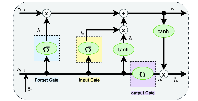
Figure 2: LSTM unit architecture.

III-B Proposed LSTM-TA Estimator

Unlike the LSTM-DNN-DPA estimator, where the LSTM and DNN networks are used for channel estimation and noise compensation respectively, the proposed estimator employs only LSTM. Moreover, the LSTM input dimension is decreased to include only $K_{on}$ subcarriers, therefore the overall computational complexity is significantly reduced. The proposed estimator proceeds as follows:

LSTM-based prediction

: The first step is to estimate the channel for the current received OFDM symbol employing the previous estimated channel $\hat{\tilde{\bm{h}}}_{\text{DL-TA}_{i-1,d}[k]}$, where the $i$-th LSTM unit input is denoted by $\tilde{\bar{{\bm{x}}}}_{{i}}\in\mathbb{R}^{2K_{on}\times 1}$, where

$$\small\bar{\bm{x}}_{i}=\left\{\begin{array}[]{ll}\hat{\tilde{\bm{h}}}_{\text{LSTM}_{i-1,d}}[k],&\quad k\in{\mathcal{K}}_{\text{d}}\\ \hat{\tilde{\bm{h}}}_{{i-1,p}}[k],&\quad k\in{\mathcal{K}}_{\text{p}}\end{array}\right..$$ (16)

$\tilde{\bar{{\bm{x}}}}_{{i}}$ is obtained by applying complex to real valued conversion to $\bar{\bm{x}}_{i}$ by stacking its real and imaginary values in one vector. We note that $\hat{\tilde{\bm{h}}}_{{i-1,p}}[k]$ denotes the least square (LS) estimated channel at the ${\mathcal{K}}_{\text{p}}$ subcarriers. After that, $\tilde{\bar{{\bm{x}}}}_{{i}}$ is processed by the LSTM unit, such that

$$\small\hat{\tilde{\bm{h}}}_{\text{LSTM}_{i,d}}=\Omega_{\text{LSTM}}(\tilde{\bar{\bm{x}}}_{i},\Theta),$$ (17)

where $\Omega_{\text{LSTM}}$ is the LSTM unit processing with overall weights denoted by $\Theta$.

DPA estimation

The LSTM estimated channel undergoes DPA estimation using the $i$-th received OFDM symbol as follows

$$\small\bm{d}_{\text{LSTM}_{i}}[k]=\mathfrak{D}\big{(}\frac{\bm{y}_{i}[k]}{\hat{\tilde{\bm{h}}}_{\text{LSTM}_{i-1}}[k]}\big{)},~{}\hat{\tilde{\bm{h}}}_{\text{LSTM}_{0}}[k]=\hat{\tilde{\bm{h}}}_{\text{LS}}[k],$$ (18)

$$\small\hat{\tilde{\bm{h}}}_{\text{LSTM-DPA}_{i}}[k]=\frac{\bm{y}_{i}[k]}{\bm{d}_{\text{LSTM}_{i}}[k]}.$$ (19)

TA processing

Finally, in order to alleviate the impact of the AWGN noise, TA processing is applied to the $\hat{\tilde{\bm{h}}}_{\text{LSTM-DPA}_{i}}[k]$ estimated channel, such that

$$\small\hat{\bar{\bm{h}}}_{\text{DL-TA}_{i,d}}=(1-\frac{1}{\alpha})\hat{\bar{\bm{h}}}_{\text{DL-TA}_{i-1,d}}+\frac{1}{\alpha}\hat{\bar{\bm{h}}}_{\text{LSTM-DPA}_{i,d}}.$$ (20)

In this paper we used a fixed $\alpha=2$ for simplicity. Therefore, the TA applied in (20) degrades the AWGN noise power $\sigma^{2}$ iteratively within the received OFDM frame according to the ratio

$$\small\begin{split}{R}_{\text{DL-TA}_{q}}&=\left(\frac{1}{4}\right)^{(q-1)}+\sum_{j=2}^{q}\left(\frac{1}{4}\right)^{(q-j+1)}=\frac{4^{q-1}+2}{3\times 4^{q-1}}.\end{split}$$ (21)

${R}_{\text{DL-TA}_{q}}$ denotes the AWGN noise power ratio of the estimated channel at the $q$-th estimated channel, where ${1<q<I+1}$ and ${{R}_{\text{DL-TA}_{1}}=1}$ denotes the AWGN noise power ratio at $\hat{\tilde{\bm{h}}}_{\text{LS}}[k]$. The full derivation of (21) is provided in Appendix A. It can be seen from the derivation of ${R}_{\text{DL-TA}_{q}}$ that the noise power is decreasing iteratively over the received OFDM frame, hence the SNR increase which leads to better overall performance.

TABLE I: Proposed LSTM parameters.

(LSTM units; Hidden size)	(1;128)
Activation function	ReLU ($y=\max(0,x)$)
Number of epochs	500
Training samples	16000
Testing samples	2000
Batch size	128
Optimizer	ADAM
Loss function	MSE
Learning rate	0.001
Training SNR	40 dB

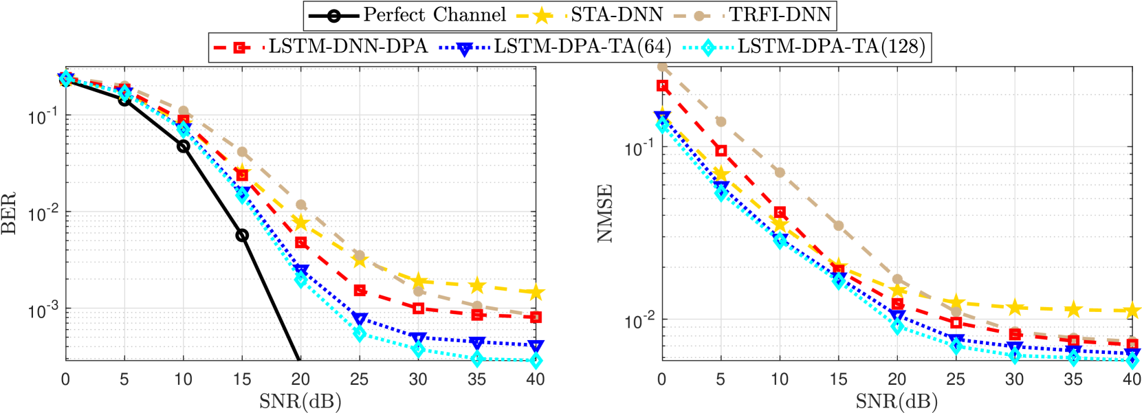
(a) BER performance employing high mobility scenario.

(b) NMSE performance employing high mobility scenario.

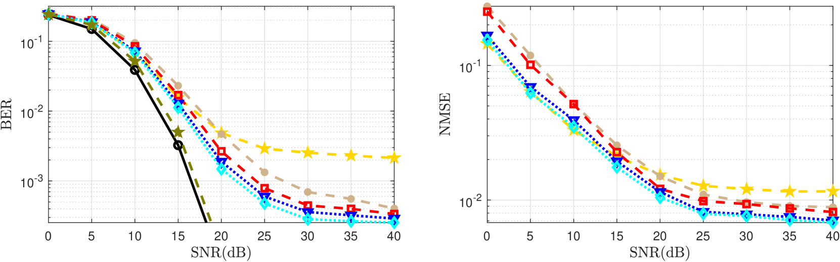
(c) BER performance employing very high mobility scenario.

(d) NMSE performance employing very high mobility scenario.

Figure 3: VTV-SDWW vehicular channel model simulation results.

The proposed LSTM training is performed using SNR = 40 dB to achieve the best performance as observed in [9], due to the fact that when the training is performed for a high SNR value, the LSTM is able to better learn the channel statistics, and due to its good generalization ability, it can still perform well in low SNR regions, where the noise is dominant. Moreover, intensive experiments are performed using the grid search algorithm [10] in order to select the best suitable LSTM hyper parameters in terms of both performance and complexity. Table. I summarizes the proposed LSTM training parameters.

IV Simulation Results

Figure 4: Computational complexity of the studied channel estimators.

In this section, BER and NMSE simulations followed by a computational complexity analysis are conducted in order to evaluate the performance of the proposed estimator compared to IEEE 802.11p DL-based estimators.

In this paper, we consider the VTV-SDWW tapped delay line (TDL) vehicular channel model [11] with two different mobility conditions: (i) High mobility: V = 100 km/hr, with Doppler shift $f_{d}$ = 550 Hz. (ii) Very high mobility: V = 200 km/hr, with $f_{d}$ = 1100 Hz. VTV-SDWW channel model represents the communication channel between two vehicles moving on a highway having center wall between its lanes, and it was obtained by a measurement campaign implemented in metropolitan Atlanta. Detailed measurement setups are provided in [12]. Concerning the simulation parameters, 16QAM modulation is employed over a frame size of $I=50$ OFDM symbols. The used channel coding is convolutional with half code rate. Moreover, three hidden layer DNN with $15$ neurons each is employed in the STA-DNN and TRFI-DNN estimators, with $\alpha=\beta=2$ as defined in [4].

IV-A BER and NMSE Performances

Fig. 3 depict the BER and NMSE performances of high and very high mobility vehicular scenarios respectively. As we can notice, the DNN-based estimators suffer from error floor, especially in high SNR region. Moreover, the LSTM-DNN-DPA estimator outperforms them in the entire SNR regions. This is explained by the high ability of the LSTM in capturing the temporal correlations of the channel more than the DNN network.

On the other hand, the proposed LSTM-DPA-TA estimator is able to outperform the LSTM-DNN-DPA estimator in high mobility scenario by $7$ dB and $5$ dB gains in terms of SNR at BER = $10^{-3}$, when $P=128$ and $P=64$ are employed respectively. We note that employing larger LSTM hidden state size, i.e $P=128$ achieves better performance than the optimized LSTM unit ($P=64$). However, in very high mobility scenario, since the temporal correlation between subsequent channel realizations significantly reduces, the proposed estimators outperform the LSTM-DNN-DPA estimator by around $3$ dB gains in terms of SNR at BER = $10^{-3}$. The proposed estimator performance gain in both scenarios is mainly due to employing the TA processing which reduces the AWGN noise significantly. Moreover, the LSTM achieves better channel estimation performance than DNN while significantly reducing the computational complexity. This can be explained by the high ability of LSTM in learning the channel time correlations, compared with a simple DNN architecture.

IV-B Computational Complexity Analysis

In general, the estimator computational complexity is expressed in terms of real-valued multiplication/division and summation/subtraction mathematical operations required to estimate the channel for one received OFDM symbol. We note that STA-DNN and TRFI-DNN achieve lower complexity compared to the LSTM-based estimators because LSTM processing requires more operations than DNN processing. Thus, in the following analysis we will focus on comparing the proposed LSTM-DPA-TA estimator with the LSTM-DNN-DPA estimator.

In [4], the authors provide a detailed computational complexity analysis of the DNN-based estimators, where the computational complexity of the DNN network denoted by $C_{\text{DNN}}$ can be expressed as follows

$$\small C_{\text{DNN}}=2\sum_{l=1}^{L+1}{N}_{l-1}{N}_{l},$$ (22)

where $L$ is the number of hidden layers within the DNN network with $N_{l}$ neurons each, and $N_{0}$, $N_{L+1}$ denote the input and output DNN network dimensions respectively.

For the computational complexity of the LSTM unit, it can be calculated in terms of the required real values operations performed by its four gates, where each gate applies $P^{2}+PK_{in}$ real-valued multiplications, and $3P+K_{in}-2$ real-valued summations. In addition to $3P$ real-valued multiplications, and $P$ real-valued summations required by (13), and (15). Therefore, the overall computational complexity for the LSTM becomes

$$\small C_{\text{LSTM}}=4(P^{2}+PK_{in}+3P+K_{in}-2)+4P.$$ (23)

The LSTM-DNN-DPA estimator employs one LSTM unit with $P=128$ and $K_{in}=112$, followed by one hidden layer DNN network with $N_{1}=40$ neurons. Finally, the LSTM-DNN-DPA estimator applies the DPA estimation which requires $18K_{d}$ real-valued multiplication/division and $8K_{d}$ real-valued summation/subtraction. Therefore, the overall computational complexity of the LSTM-DNN-DPA estimator is $512K_{\text{in}}+98K_{d}+71040$ real-valued multiplication/division and $4K_{\text{in}}+88K_{d}+6776$ real-valued summation/subtraction.

For the proposed LSTM-DPA-TA estimator, it employs one LSTM unit with $P=128$ as LSTM-DNN-DPA estimator, or $P=64$ when the optimized LSTM unit architecture is employed. Moreover, the proposed estimator uses $K_{in}=2K_{on}$, and applies TA as a noise alleviation technique to the $\hat{\bar{\bm{h}}}_{\text{LSTM-DPA}_{i,d}}$ estimated channel, that requires only $2K_{on}$ real-valued multiplication/division and $2K_{on}$ real-valued summation/subtraction. As a results, the proposed LSTM-DPA-TA estimator requires $4P^{2}+P(8K_{on}+3)+18K_{d}+2K_{on}$ real-valued multiplication/division and $13P+10K_{on}+8K_{d}-8$ real-valued summation/subtraction.

Based on this analysis, the proposed estimator achieves less computational complexity compared to the LSTM-DNN-DPA estimator. It records $9.73\%$ and $77.63\%$ computational complexity decrease in the required real-valued multiplication/division and summation/subtraction respectively, when the LSTM unit is employed with $P=128$ hidden size. On the other hand, more complexity reduction can be achieved when the optimized LSTM unit is used with $P=64$ hidden size, where the proposed estimator is able to decrease the complexity of the required multiplication/division and summation/subtraction by $66.81\%$ and $84.90\%$ respectively. It is worth mentioning that replacing the DNN network by the TA processing in order to alleviate the AWGN noise is the main factor in decreasing the overall computational complexity, where the proposed estimator outperforms the LSTM-DNN-DPA estimator while recording a significant computational complexity reduction. Fig. 4 shows a detailed computational analysis of the benchmarked estimators in terms of real-valued operations.

V Conclusion

In this paper, we have investigated the channel estimation challenge in vehicular environments. This challenge arises from the doubly selective nature of the vehicular channel, especially in high mobility scenarios. The recently proposed DL-based IEEE 802.11p estimators have been presented and their limitations have been discussed. In order to overcome these limitations, we have proposed an LSTM-based estimator, that employs an LSTM unit for channel estimation, and a TA processing as a noise alleviation technique. Simulation results have shown the performance superiority of the proposed LSTM-DPA-TA estimator over the recently proposed DL-based estimators, while recording a significant reduction in computational complexity.

-A TA noise power alleviation ratio

According to the TA processing applied in (20), and assuming that the noise terms of consecutive symbols are uncorrelated, the noise power for the $q$-th estimated channel is expressed as follows

$$\small{R}_{\text{DL-TA}_{q}}=\mathrm{E}\left[\left\lVert\frac{\tilde{\bm{v}}_{{q-1}}}{2}+\frac{\tilde{\bm{v}}_{{q}}}{2}\right\rVert^{2}\right]=\frac{\sigma_{{q-1}}^{2}}{4}+\frac{\sigma_{{q}}^{2}}{4}.$$ (24)

Where $\tilde{\bm{v}}_{{q}}$ denotes the AWGN noise at the $q$-th received OFDM symbol. We consider that $\hat{\bar{\bm{h}}}_{\text{DL-TA}_{1}}=\hat{\tilde{\bm{h}}}_{\text{LS}}$, therefore the noise power of the first estimated channel is $\sigma^{2}$, and the noise power enhancement ratio for the successive estimated channels can be computed as follows

$$\small{R}_{\text{DL-TA}_{q}}=\left\{\begin{array}[]{ll}1,&\quad q=1\\ \\ \frac{1}{4}+\frac{1}{4}=\frac{1}{2},&\quad q=2\\ \\ \frac{\bm{R}_{\text{DL-TA}_{q-1}}}{4}+\frac{1}{4},&\quad 3<q\leq I+1\end{array}\right.$$ (25)

The generalization formula of (25) can be written as a sequence where the first element ${R}_{\text{DL-TA}_{1}}=1$ as follows

$$\small\begin{split}{R}_{\text{DL-TA}_{q}}&=\frac{1}{4}{R}_{\text{DL-TA}_{q-1}}+\frac{1}{4}=\frac{1}{4}\left({R}_{\text{DL-TA}_{q-1}}+1\right)\\ &=\frac{1}{4}\left(\frac{1}{4}{R}_{\text{DL-TA}_{q-2}}+\frac{1}{4}+1\right)\\ &=\frac{1}{4}\left(\frac{1}{4}\left(\frac{1}{4}R_{\text{DL-TA}_{q-3}}+\frac{1}{4}\right)+\frac{1}{4}+1\right)\\ &=\frac{1}{4}\left(\frac{1}{4^{(q-1)-1}}{{R}}_{\text{DL-TA}_{q-(q-1)}}+\frac{1}{4^{(q-1)-1}}+\dots+\frac{1}{4^{0}}\right)\\ &=\frac{1}{4}\left(\frac{1}{4^{q-2}}{{R}}_{\text{DL-TA}_{1}}+\frac{1}{4^{q-2}}+\frac{1}{4^{q-3}}+\dots+\frac{1}{4^{0}}\right)\\ &=\frac{1}{4}\left(\frac{1}{4^{q-2}}+\frac{1}{4^{q-2}}+\frac{1}{4^{q-3}}+\dots+\frac{1}{4^{0}}\right).\end{split}$$ (26)

The sequence derived in (26) can be written as follows:

$$\small{R}_{\text{DL-TA}_{q}}=\frac{1}{4}\left(\frac{1}{4^{q-2}}+\sum_{j=2}^{q}\left({\frac{1}{4}}\right)^{q-j}\right).$$ (27)

Let $j^{\prime}=q-j$, then (27) can be written in terms of $j^{\prime}$ according to the summation of geometric sequence rule [13] such that

$$\small{R}_{\text{DL-TA}_{q}}=\frac{1}{4}\left(\frac{1}{4^{q-2}}+\sum_{j^{\prime}=0}^{q-2}\left({\frac{1}{4}}\right)^{j^{\prime}}\right)=\frac{4^{q-1}+2}{3\times 4^{q-1}}.$$ (28)

References

- [1] P. Alexander, D. Haley, and A. Grant, “Cooperative Intelligent Transport Systems: 5.9-GHz Field Trials,” Proceedings of the IEEE, vol. 99, no. 7, pp. 1213–1235, 2011.
- [2] J. A. Fernandez, K. Borries, L. Cheng, B. V. K. Vijaya Kumar, D. D. Stancil, and F. Bai, “Performance of the 802.11p Physical Layer in Vehicle-to-Vehicle Environments,” IEEE Transactions on Vehicular Technology, vol. 61, no. 1, pp. 3–14, 2012.
- [3] Yoon-Kyeong Kim, Jang-Mi Oh, Yoo-Ho Shin, and Cheol Mun, “Time and Frequency Domain Channel Estimation Scheme for IEEE 802.11p,” in 17th International IEEE Conference on Intelligent Transportation Systems (ITSC), 2014, pp. 1085–1090.
- [4] A. K. Gizzini, M. Chafii, A. Nimr, and G. Fettweis, “Deep Learning Based Channel Estimation Schemes for IEEE 802.11p Standard,” IEEE Access, vol. 8, pp. 113 751–113 765, 2020.
- [5] A. K. Gizzini, M. Chafii, A. Nimr, and G. Fettweis, “Joint TRFI and Deep Learning for Vehicular Channel Estimation,” in 2020 IEEE Globecom Workshops (GC Wkshps, 2020, pp. 1–6.
- [6] J. Pan, H. Shan, R. Li, Y. Wu, W. Wua, and T. Q. S. Quek, “Channel Estimation Based on Deep Learning in Vehicle-to-everything Environments,” IEEE Communications Letters, pp. 1–1, 2021.
- [7] A. Abdelgader and L. Wu, “The Physical Layer of the IEEE 802.11 p WAVE Communication Standard: The Specifications and Challenges,” in The Physical Layer of the IEEE 802.11 p WAVE Communication Standard: The Specifications and Challenges, vol. 2, 10 2014.
- [8] K. Greff, R. K. Srivastava, J. Koutník, B. R. Steunebrink, and J. Schmidhuber, “LSTM: A Search Space Odyssey,” IEEE Transactions on Neural Networks and Learning Systems, vol. 28, no. 10, pp. 2222–2232, 2017.
- [9] A. K. Gizzini, M. Chafii, A. Nimr, and G. Fettweis, “Enhancing Least Square Channel Estimation Using Deep Learning,” in 2020 IEEE 91st Vehicular Technology Conference (VTC2020-Spring), 2020, pp. 1–5.
- [10] F. Pontes, G. Amorim, P. Balestrassi, A. Paiva, and J. Ferreira, “Design of Experiments and Focused Grid Search for Neural Network Parameter Optimization,” Neurocomputing, vol. 186, pp. 22 – 34, 2016.
- [11] G. Acosta-Marum and M. A. Ingram, “Six Time and Frequency Selective Empirical Channel Models for Vehicular Wireless LANs,” IEEE Vehicular Technology Magazine, vol. 2, no. 4, pp. 4–11, 2007.
- [12] G. Acosta-Marum, “Measurement, Modeling, and OFDM Synchronization for the Wideband Mobile-to-Mobile Channel,” Ph.D. dissertation, Georgia Inst. Technol., Atlanta, GA, 2007.
- [13] G. Orosi, “The Arithmetico-Geometric Sequence: an Application of Linear Algebra,” International Journal of Mathematical Education in Science and Technology, vol. 47, no. 5, pp. 766–772, 2016.