Energy Conservation in the thin-layer approximation: V. The surface brightness in supernova remnants

Abstract

Two new equations of motion for a supernova remnant (SNR) are derived in the framework of energy conservation for the thin-layer approximation. The first one is based on an inverse square law for the surrounding density and the second one on a non-cubic dependence of the swept mass. Under the assumption that the observed radio-flux scales as the flux of kinetic energy, two scaling laws are derived for the temporal evolution of the surface brightness of SNRs. The astrophysical applications cover two galactic samples of surface brightness and an extragalactic one.

Keywords: ISM: supernova remnants, radio continuum: galaxies

1 Introduction

The surface brightness versus diameter, ($\Sigma-D\leavevmode\nobreak\$), for supernova remnants (SNRs) were initially analysed from a theoretical point of view in the framework of the initial conditions for the time evolution of SNRs [1, 2, 3, 4]. Some generic information on $\Sigma-D\leavevmode\nobreak\$can be found in reviews of SNRs [5, 6].

The astrophysical approach to the $\Sigma-D\leavevmode\nobreak\$has always mixed the observations with the theory and the statistics. We select some items among others: a catalogue of 25 SNRs has been compiled by [7] with the conclusion that SNRs in the galactic halo have diameters greater than those in the disk, the evolutionary properties of SNRs have been deduced from observations with the Molonglo and Parkes radio telescopes [8], the $\Sigma-D\leavevmode\nobreak\$relationship was used to fix the scale for distances of SNRs [9], the diameters, luminosities, surface brightness, galactic heights for 231 SNRs were processed in the framework of the Sedov solution [10], a new high-latitude SNR [11] was analysed, an updated radio $\Sigma-D\leavevmode\nobreak\$relationship was derived [12] and the phases of some supernova remnant have been determined from the observations [13]. In order to derive the $\Sigma-D\leavevmode\nobreak\$relationship some hypotheses on the single equation of motion should be made, e.g., the conservation of the momentum [14]. Here conversely we will apply the energy conservation in the framework of the thin-layer approximation and we will derive an analytical expression for the $\Sigma-D\leavevmode\nobreak\$relationship. This paper derives two new equations of motion in the framework of energy conservation for the thin-layer approximation, see Section 2, applies the two analytical expressions for the surface brightness to two galactic samples, see Section 3, and to an extragalactic catalog, see Section 4.

2 The equations of motion

The conservation of kinetic energy in spherical coordinates in the framework of the thin-layer approximation, here taken to be an assumption, states that

$$\frac{1}{2}M_{0}(r_{0})\,v_{0}^{2}=\frac{1}{2}M(r)\,v^{2}\quad,$$ (1)

where $M_{0}(r_{0})$ and $M(r)$ are the swept masses at $r_{0}$ and $r$, while $v_{0}$ and $v$ are the velocities of the thin layer at $r_{0}$ and $r$. We now present two equations of motion for SNRs and the back-reaction for one of the two.

2.1 The inverse square law

The medium around the SN is assumed to scale as an inverse square law

$$\rho(r;r_{0})=\{\begin{array}[]{ll}\rho_{c}&\mbox{if $r\leq r_{0}$ }\\ \rho_{c}(\frac{r_{0}}{r})^{2}&\mbox{if $r>r_{0}$.}\end{array},$$ (2)

where $\rho_{c}$ is the density at $r=0$ and $r_{0}$ is the radius after which the density starts to decrease. When the conservation of energy is applied the velocity as a function of the radius is

$$v(r;r_{0},v_{0})=-{\frac{\sqrt{-\left(2\,r_{{0}}-3\,r\right)r_{{0}}}v_{{0}}}{2\,r_{{0}}-3\,r}}\quad.$$ (3)

The trajectory, i.e. the radius as a function of time, is

$$r(t;t_{0},r_{0},v_{0})=\frac{1}{6}\,\sqrt[3]{2}\sqrt[3]{r_{{0}}}\left(\left(9\,t-9\,t_{{0}}\right)v_{{0}}+2\,r_{{0}}\right)^{2/3}+\frac{2}{3}\,r_{{0}}\quad,$$ (4)

and the velocity as a function of time is

$$v(t;t_{0},r_{0},v_{0})={\frac{\sqrt[3]{2}\sqrt[3]{r_{{0}}}v_{{0}}}{\sqrt[3]{\left(9\,t-9\,t_{{0}}\right)v_{{0}}+2\,r_{{0}}}}}\quad.$$ (5)

More details can be found in [15]. The rate of transfer of mechanical energy, $L_{m}$, is

$$L_{m}(t)=\frac{1}{2}\rho(t)4\pi r(t)^{2}v(t)^{3}\quad,$$ (6)

where $\rho(t)$,$r(t)$ and $v(t)$ are the instantaneous density, radius and velocity of the SN. We now assume that the density in front of the advancing expansion scales as

$$\rho(t)=\rho_{0}(\frac{r_{0}}{r(t)})^{d}\quad,$$ (7)

where $r_{0}$ is the radius at $t_{0}$ and $d$ is a parameter which allows matching the observations. The mechanical luminosity is now

$$L_{m}(t)=\frac{1}{2}\rho_{0}(\frac{r_{0}}{r(t)})^{d}4\pi r(t)^{2}v(t)^{3}\quad.$$ (8)

In the case here analysed of the inverse square profile for density we have

$$L_{m}(t;v_{0},t_{0},r_{0})=\frac{DLM}{81\,v_{{0}}t-81\,v_{{0}}t_{{0}}+18\,r_{{0}}}\quad,$$ (9)

where

$$DLM=\rho_{{0}}{6}^{d}\left({r_{{0}}\left(\sqrt[3]{2}\sqrt[3]{r_{{0}}}\left(\left(9\,t-9\,t_{{0}}\right)v_{{0}}+2\,r_{{0}}\right)^{{\frac{2}{3}}}+4\,r_{{0}}\right)^{-1}}\right)^{d}$$

$$\times\pi\,\left(\sqrt[3]{2}\sqrt[3]{r_{{0}}}\left(\left(9\,t-9\,t_{{0}}\right)v_{{0}}+2\,r_{{0}}\right)^{{\frac{2}{3}}}+4\,r_{{0}}\right)^{2}r_{{0}}{v_{{0}}}^{3}\quad.$$ (10)

We now assume that the observed luminosity, $L_{\nu}$, in a given band denoted by the frequency $\nu$ is proportional to the mechanical luminosity

$$L_{\nu}(t)=cost*L_{m}(t)\quad,$$ (11)

where $L_{\nu}$ is the observed radio luminosity in a given band and $cost$ a constant which resolves the mismatch between theory and observations. The surface brightness is the luminosity divided by the interested area

$$\Sigma=\frac{L_{\nu}(t)}{\pi r(t)^{2}}\quad,$$ (12)

which is

$$\Sigma(t;v_{0},t_{0},r_{0})={\it cost}\frac{4\,\,\rho_{{0}}{6}^{d}\left({\frac{r_{{0}}}{\sqrt[3]{2}\sqrt[3]{r_{{0}}}\left(\left(9\,t-9\,t_{{0}}\right)v_{{0}}+2\,r_{{0}}\right)^{2/3}+4\,r_{{0}}}}\right)^{d}r_{{0}}{v_{{0}}}^{3}}{9\,v_{{0}}t-9\,v_{{0}}t_{{0}}+2\,r_{{0}}}\quad.$$ (13)

2.2 Non cubic dependence

The swept mass is assumed to scale as

$$M(r;r_{0},\delta)=\Bigg{\{}\begin{array}[]{ll}M_{0}&\mbox{if $r\leq r_{0}$ }\\ M_{0}(\frac{r}{r_{0}})^{\delta}&\mbox{if $r>r_{0}$}\end{array},$$ (14)

where $M_{0}$ is the swept mass at $r=r_{0}$, and $\delta$ is a regulating parameter less than 3. The differential equation of the first order which regulates the motion is obtained by inserting the above $M(r)$ in equation (1)

$$\frac{dr(t;r_{0},v_{0},\delta)}{dt}=\frac{v_{{0}}}{\sqrt{{r}^{\delta}{r_{{0}}}^{-\delta}}}\quad,$$ (15)

which has as the solution

$$r(t;r_{0},v_{0},\delta)=\exp{\Bigg{(}\frac{ER}{\delta+2}\Bigg{)}}$$ (16)

where

$$ER=\ln\Big{(}{r_{{0}}}^{\delta+1}\delta\,tv_{{0}}-{r_{{0}}}^{\delta+1}\delta\,t_{{0}}v_{{0}}+2\,{r_{{0}}}^{\delta+1}tv_{{0}}$$

$$-2\,{r_{{0}}}^{\delta+1}t_{{0}}v_{{0}}+{r_{{0}}}^{\delta+2}+{\frac{{r_{{0}}}^{\delta}{\delta}^{2}{t}^{2}{v_{{0}}}^{2}}{4}}-{\frac{{r_{{0}}}^{\delta}{\delta}^{2}tt_{{0}}{v_{{0}}}^{2}}{2}}+{\frac{{r_{{0}}}^{\delta}{\delta}^{2}{t_{{0}}}^{2}{v_{{0}}}^{2}}{4}}$$

$$+{r_{{0}}}^{\delta}\delta\,{t}^{2}{v_{{0}}}^{2}-2\,{r_{{0}}}^{\delta}\delta\,tt_{{0}}{v_{{0}}}^{2}+{r_{{0}}}^{\delta}\delta\,{t_{{0}}}^{2}{v_{{0}}}^{2}+{r_{{0}}}^{\delta}{t}^{2}{v_{{0}}}^{2}-2\,{r_{{0}}}^{\delta}tt_{{0}}{v_{{0}}}^{2}+{r_{{0}}}^{\delta}{t_{{0}}}^{2}{v_{{0}}}^{2}\Big{)}\quad.$$ (17)

The velocity is

$$v(t;r_{0},v_{0},\delta)=\frac{NV}{\left(\delta+2\right)\left(\delta\,tv_{{0}}-\delta\,t_{{0}}v_{{0}}+2\,tv_{{0}}-2\,t_{{0}}v_{{0}}+2\,r_{{0}}\right)^{2}}$$ (18)

where

$$NV=v_{{0}}\left({r_{{0}}}^{\delta}\left(v_{{0}}\left(\delta+2\right)\left(t-t_{{0}}\right)+2\,r_{{0}}\right)^{2}\right)^{\left(\delta+2\right)^{-1}}$$

$$\times\Big{(}2\,{4}^{-\left(\delta+2\right)^{-1}}{\delta}^{2}tv_{{0}}-2\,{4}^{-\left(\delta+2\right)^{-1}}{\delta}^{2}t_{{0}}v_{{0}}+8\,{4}^{-\left(\delta+2\right)^{-1}}\delta\,tv_{{0}}-8\,{4}^{-\left(\delta+2\right)^{-1}}\delta\,t_{{0}}v_{{0}}+{4}^{{\frac{\delta+1}{\delta+2}}}\delta\,r_{{0}}$$

$$+8\,{4}^{-\left(\delta+2\right)^{-1}}tv_{{0}}-8\,{4}^{-\left(\delta+2\right)^{-1}}t_{{0}}v_{{0}}+8\,{4}^{-\left(\delta+2\right)^{-1}}r_{{0}}\Big{)}\quad.$$ (19)

Figure 1 reports the analytical solution for the NCD case as given by equation (16) for SN 1993J .

Figure 1: Analytical solution for the NCD case with parameters $r_{0}=0.006\,pc$, $v_{0}=10000\,km/s$, $t_{0}=0.026\,yr$ and $\delta=0.2$, which gives $\chi^{2}=3751$. The astronomical data of SN 1993J  are represented with vertical error bars.

The mechanical luminosity is assumed to scale as in equation (8) and therefore in the NCD case is

$$L_{m}(t;r_{0},v_{0},t_{0},\delta)=$$

$$16\,{\frac{{{\rm e}^{{\it EA}}}{v_{{0}}}^{3}\left(r_{{0}}{{\rm e}^{{\it EB}}}\right)^{d}\pi\,\rho_{{0}}}{\left(\delta+2\right)^{3}\left(v_{{0}}\left(\delta+2\right)\left(t-t_{{0}}\right)+2\,r_{{0}}\right)^{6}}{S_{{2}}}^{3\,\left(\delta+2\right)^{-1}}\left(S_{{1}}{4}^{{\frac{\delta+1}{\delta+2}}}+{4}^{-\left(\delta+2\right)^{-1}}v_{{0}}{\delta}^{2}\left(t-t_{{0}}\right)\right)^{3}}\quad,$$ (20)

where

$$EA=\frac{1}{\delta+2}\Big{(}{-4\,\ln(2)+2\,\ln(4\,v_{{0}}(\delta+2)(t-t_{{0}}){r_{{0}}}^{\delta+1}+4\,{r_{{0}}}^{\delta+2}+(({t}^{2}-2\,tt_{{0}}+{t_{{0}}}^{2}){\delta}^{2}}$$

$${+(4\,{t}^{2}-8\,tt_{{0}}+4\,{t_{{0}}}^{2})\delta+4\,{t}^{2}-8\,tt_{{0}}+4\,{t_{{0}}}^{2}){v_{{0}}}^{2}{r_{{0}}}^{\delta})}\Big{)}\quad,$$ (21)

and

$$EB={\frac{2\,\ln\left(2\right)-\ln\left(\left(v_{{0}}\left(\delta+2\right)\left(t-t_{{0}}\right)+2\,r_{{0}}\right)^{2}{r_{{0}}}^{\delta}\right)}{\delta+2}}\quad,$$ (22)

$$S_{1}=\left(\delta+1\right)\left(t-t_{{0}}\right)v_{{0}}+{\frac{r_{{0}}\left(\delta+2\right)}{2}}\quad,$$ (23)

and

$$S_{2}=\left(v_{{0}}\left(\delta+2\right)\left(t-t_{{0}}\right)+2\,r_{{0}}\right)^{2}{r_{{0}}}^{\delta}\quad.$$ (24)

The surface brightness is derived according to equation (12) and in the NCD case is

$$\Sigma(t;r_{0},v_{0},t_{0},\delta)=$$

$${\it cost}\frac{16\,\rho_{{0}}\left({4}^{-\left(\delta+2\right)^{-1}}v_{{0}}{\delta}^{2}t-{4}^{-\left(\delta+2\right)^{-1}}v_{{0}}{\delta}^{2}t_{{0}}+{\it SC}\,{4}^{{\frac{\delta+1}{\delta+2}}}\right)^{3}{{\rm e}^{{\it SA}}}\,{v_{{0}}}^{3}{r_{{0}}}^{{\frac{\left(d+3\right)\delta+2\,d}{\delta+2}}}{{\it SB}}^{{\frac{-6-6\,\delta}{\delta+2}}}}{\left(\delta+2\right)^{3}}\quad,$$ (25)

where

$$SA=-{\frac{d\left(-2\,\ln\left(2\right)+2\,\ln\left(v_{{0}}\left(\delta+2\right)\left(t-t_{{0}}\right)+2\,r_{{0}}\right)+\delta\,\ln\left(r_{{0}}\right)\right)}{\delta+2}}\quad,$$ (26)

$$SB=v_{{0}}\left(\delta+2\right)\left(t-t_{{0}}\right)+2\,r_{{0}}$$ (27)

and

$$SC=\left(\delta+1\right)\left(t-t_{{0}}\right)v_{{0}}+{\frac{r_{{0}}\left(\delta+2\right)}{2}}\quad.$$ (28)

A comparison of the two models here implemented for the trajectory is reported in Figure 2.

Figure 2: Analytical solution for the inverse square model (dashed line) when $r_{0}=1\,pc$, $v_{0}=4000\,km/s$, $t_{0}=10\,yr$, and NCD model (full line ) with the same parameters and $\delta=1.3$.

2.3 Non cubic dependence and back reaction

The radiative losses per unit length are assumed to be proportional to the flux of momentum as an assumption

$$-\epsilon\rho_{s}v^{2}4\,\pi r^{2}\quad,$$ (29)

where $\epsilon$ is a constant and $rho_{s}$ is the density in the thin advancing layer.

The volume, $V$, of the advancing layer is

$$V=4\pi r^{2}\Delta\,r$$ (30)

with $\Delta r=r/12$, therefore the above density for the advancing layer is

$$\rho_{s}=\frac{M(r;r_{0},\delta)}{V}\quad.$$ (31)

Inserting in the above equation the velocity to the first order as given by equation (18) the radiative losses, $Q(r;r_{0},v_{0},\delta,\epsilon)$, are

$$Q(r;r_{0},v_{0},\delta,\epsilon)=-12\,{\frac{\epsilon\,M_{{0}}{v_{{0}}}^{2}}{r}}\quad.$$ (32)

The sum of the radiative losses between $r_{0}$ and $r$ is given by the following integral, $L$,

$$L(r;r_{0},v_{0},\delta,\epsilon)=\int_{r_{0}}^{r}Q(r;r_{0},v_{0},\delta,\epsilon)dr=-12\,\epsilon\,M_{{0}}{v_{{0}}}^{2}\ln\left(r\right)+12\,\epsilon\,M_{{0}}{v_{{0}}}^{2}\ln\left(r_{{0}}\right)\quad.$$ (33)

The conservation of energy in the presence of the back reaction due to the radiative losses is

$${\frac{2\,\pi\,{r_{{0}}}^{3}{v}^{2}}{3}\left({\frac{r}{r_{{0}}}}\right)^{\delta}}+16\,\epsilon\,\pi\,{r_{{0}}}^{3}{v_{{0}}}^{2}\ln\left(r\right)-16\,\epsilon\,\pi\,{r_{{0}}}^{3}{v_{{0}}}^{2}\ln\left(r_{{0}}\right)={\frac{2\,\pi\,{r_{{0}}}^{3}{v_{{0}}}^{2}}{3}}\quad.$$ (34)

An analytical solution for the velocity to second order, $v_{c}(r;r_{0},c_{0},\delta,\epsilon)$, is

$$v_{c}(r;r_{0},v_{0},\delta,\epsilon)={r}^{-{\frac{\delta}{2}}}{r_{{0}}}^{{\frac{\delta}{2}}}\sqrt{24\,\ln\left(r_{{0}}\right)\epsilon-24\,\ln\left(r\right)\epsilon+1}v_{{0}}\quad.$$ (35)

The inclusion of the back reaction allows the evaluation of the SRS’s maximum length, $r_{back}(r_{0},\delta,\epsilon)$ , which can be derived by setting the above velocity equal to zero.

$$r_{back}(r_{0},\delta,\epsilon)={{\rm e}^{{\frac{24\,\ln\left(r_{{0}}\right)\epsilon+1}{24\,\epsilon}}}}\quad.$$ (36)

Figure 3 reports the finite radius of the advancing SNR as a function of $\epsilon$.

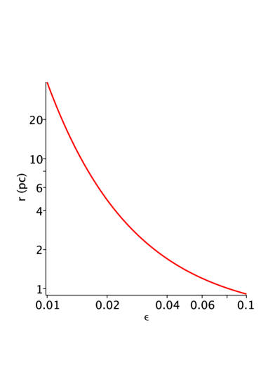
Figure 3: Length of the SNR, $r_{back}$, when $r_{0}=0.6pc$ as function of $\epsilon$.

3 Galactic Application

In the following we will process a sample of data $x_{i},y_{i}$ with $i$ varying between 1 and $N$ by a power law fit of the the type

$$y(x)=C\,x^{\alpha}\quad,$$ (37)

where $C$ and $\alpha$ are two constants to be found from the sample.

The first source for the observed $\Sigma-D\leavevmode\nobreak\$relationship for the SNRs of our galaxy can be found in Figure 3 of [10] which is now digitized, see Figure 4.

Figure 4: Observed $\Sigma-D\leavevmode\nobreak\$relationship (empty stars) and fitted power law (full line) with parameters as in Table 1.

Table 1 reports the minimum diameter, $D_{min}$, the average diameter, $\overline{D}$, the maximum diameter, $D_{max}$, the minimum $\Sigma-D\leavevmode\nobreak\$, $\Sigma-D_{min}$, the average $\Sigma-D\leavevmode\nobreak\$, $\overline{\Sigma-D}$ and the maximum $\Sigma-D\leavevmode\nobreak\$, $\Sigma-D_{max}$ as well as the two parameters of the power law fit.

Table 1: Statistics of the observed $\Sigma-D\leavevmode\nobreak\$galactic relationship and the two parameters of the power law fit. The theoretical parameters of the inverse square solution are $r_{0}=1\,pc$, $v_{0}=4000\,km/s$, $d=1.1$, $t_{0}=10\,yr$, $t_{min}=2\,t_{0}$ and $t_{max}=2.05\,10^{5}$yr.

$$\begin{array}[]{lll}\hline\cr\hline\cr\vskip 3.0pt plus 1.0pt minus 1.0pt\cr parameter&observed&theoretical\\ \vskip 3.0pt plus 1.0pt minus 1.0pt\cr\hline\cr\vskip 3.0pt plus 1.0pt minus 1.0pt\cr D_{min}(pc)&1.18&3.44\\ \overline{D}(pc)&37.17&37.4\\ D_{max}(pc)&227.17&86.708\\ \Sigma_{min}(pc)&5.96\,10^{-23}&3\,10^{-20}\\ \overline{\Sigma}(pc)&2.16\,10^{-19}&2.24\,10^{-19}\\ \Sigma_{max}(pc)&1.66\,10^{-17}&2.54\,10^{-18}\\ C&3.83\,10^{-19}&1.32\,10^{-17}\\ \alpha&-1.32&-1.33\\ \vskip 3.0pt plus 1.0pt minus 1.0pt\cr\hline\cr\end{array}$$

A second source for the $\Sigma-D\leavevmode\nobreak\$relationship is the Green’s catalog [16] where the flux density in $Jy$ at $1\,GHz$, $S_{1}$, and the mayor and minor angular size in arcmin, $\theta$, are reported for 295 SNRs. The surface-brightness in SI is

$$\Sigma=1.181\,10^{-19}\frac{S_{1}}{\theta}\frac{W}{m^{2}\,Hz\,sr}\quad SI\quad,$$ (38)

but after [8] the radio astronomers use the following conversion

$$\Sigma=1.505\,10^{-19}\frac{S_{1}}{\theta}\frac{W}{m^{2}\,Hz\,sr}\quad astronomy\quad,$$ (39)

which will also be adopted here.

The probability density function (PDF), $p(z)$, to have an SNR as a function of the galactic height $z$ is characterized by an exponential PDF

$$p(z)=\frac{1}{b}\exp{-\frac{z}{b}}\quad,$$ (40)

with $b=83$ pc [10]. The linear diameter ($D$) of an SNR increases with the galactic height see Figure 2 in [10] and in the framework of the model with an inverse square law model for density the parameter $r_{0}$ is chosen to have the following dependence with the the galactic height

$$r_{0}=0.01+0.5(\frac{z}{z_{max}})\quad,$$ (41)

where $z_{max}=687$ is the maximum galactic height which belongs to an SNR. The above assumption coupled with an initial velocity for the inverse square law model for density of $v_{0}=4000\frac{km}{s}$ for all the SNRs will ensure a longer radius for SNRs with higher galactic heights, see Figure 5.

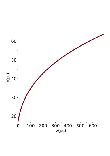
Figure 5: Theoretical radius as given by the inverse square model, see Eq. (5), as function of the galactic height; $v_{0}=4000\,\frac{km}{s}$, $t_{0}=10\,yr$ and $t=5\,10^{4}yr$.

We now simulate the galactic $\Sigma-D\leavevmode\nobreak\$relationship for a number of theoretical SNRs, $N$, equal to that observed according to the following rules

1. We randomly generate $N$ parameters $z$ according to the exponential PDF (40)

2. At each random value of $z$ we associate an initial parameter $r_{0}$ according to the empirical equation (41)

3. We randomly generate $N$ times, $t$, according to the uniform distribution between a minimum value of time, $t_{min}$ and a maximum value of time, $t_{max}$.

4. Given the parameters $r_{0}$, $v_{0}$, $t_{0}$ and $t$ we evaluate the radius according to equation (4) for an inverse power law profile for density. The diameter is obtained doubling the above result.

5. $\Sigma$ is now generated according to equation (13) once the regulating parameter $d$ is provided

The theoretical display of the results is reported in Figure 6, were we matched the three main parameters ($\overline{D}(pc),\overline{\Sigma-D},\alpha$) which for the observations are ($37.17,2.16\,10^{-19},-1.32$) and for our simulation are ($37.4,2.24\,10^{-19},-1.33$).

Figure 6: Theoretical $\Sigma-D\leavevmode\nobreak\$relationship (empty stars) and fitted power law (full line) with parameters as in Table 1.

The surface brightness of the Green’s catalog is reported in Figure 7 and our simulation in Figure 8; see also Table 2 for a comparison between the data of the catalog and the simulation.

Figure 7: Histogram of the $\Sigma-D\leavevmode\nobreak\$for 294 SNR as derived from the Green’s catalog [16].

Figure 8: Histogram for the $\Sigma-D\leavevmode\nobreak\$of our simulation in the framework of the inverse square model.

Table 2: Statistics of the observed [16] and simulated $\Sigma$ in the framework of the inverse square model.

$$\begin{array}[]{lll}\hline\cr\hline\cr\vskip 3.0pt plus 1.0pt minus 1.0pt\cr parameter&observed&theoretical\\ \vskip 3.0pt plus 1.0pt minus 1.0pt\cr\hline\cr\vskip 3.0pt plus 1.0pt minus 1.0pt\cr\Sigma_{min}(pc)&1.42\,10^{-25}&1.27\,10^{-21}\\ \overline{\Sigma}(pc)&1.13\,10^{-18}&1.13\,10^{-18}\\ \Sigma_{max}(pc)&4.34\,10^{-17}&6.17\,10^{-17}\\ \vskip 3.0pt plus 1.0pt minus 1.0pt\cr\hline\cr\end{array}$$

4 Extragalactic Application

A sample of SNRs in nearby galaxies with diameter in pc and flux at 1.4 GHz in mJy has been collected [17]. The connected catalog is available at http://cdsweb.u-strasbg.fr/. The statistics of the $\Sigma-D\leavevmode\nobreak\$relationship for this extragalactic sample is reported in Table 3 and displayed in Figure 9.

Table 3: Statistics of the observed $\Sigma-D\leavevmode\nobreak\$extragalactic relationship and the two parameters of the power law fit. The theoretical parameters for the NCD case are $r_{0}=1\,pc$, $r_{0,min}=2\,r_{0}$, $r_{0,max}=1.4\,r_{0,min}$, $v_{0}=4000\,km/s$, $\delta=1.3$, $d=1.1$, $t_{0}=10\,yr$, $t_{min}=2\,t_{0}$ and $t_{max}=2.9\,10^{4}$yr.

$$\begin{array}[]{lll}\hline\cr\hline\cr\vskip 3.0pt plus 1.0pt minus 1.0pt\cr parameter&observed&theoretical\\ \vskip 3.0pt plus 1.0pt minus 1.0pt\cr\hline\cr\vskip 3.0pt plus 1.0pt minus 1.0pt\cr D_{min}(pc)&0.51&4.05\\ \overline{D}(pc)&34.6&34.23\\ D_{max}(pc)&450&54.39\\ \Sigma_{min}(pc)&2.4\,10^{-22}&1.87\,10^{-17}\\ \overline{\Sigma}(pc)&6.13\,10^{-16}&8.82\,10^{-16}\\ \Sigma_{max}(pc)&8.6\,10^{-14}&4.14\,10^{-14}\\ C&8.85\,10^{-16}&2.64\,10^{-12}\\ \alpha&-3.1&-2.96\\ \vskip 3.0pt plus 1.0pt minus 1.0pt\cr\hline\cr\end{array}$$

Figure 9: Observed $\Sigma-D\leavevmode\nobreak\$relationship for the extragalactic case (empty stars) and fitting power law (full line) with parameters as in Table 3.

The theoretical $\Sigma-D\leavevmode\nobreak\$is now evaluated in the framework of the NCD model, see equation (25), with a numerical procedure which is similar to that of the galactic case but with the difference that there is no dependence of $r_{0}$ on $z$. The numerical value of $r_{0}$ in the extragalactic case is now randomly generated according to the uniform distribution between a minimum value, $r_{0,min}$, and a maximum value, $r_{0,max}$, see Table 3 and Figure 10.

Figure 10: Theoretical $\Sigma-D\leavevmode\nobreak\$relationship for the extragalactic case in the framework of the NCD model (empty stars) and fitting power law (full line) with parameters as in Table 3.

5 Conclusions

When an analytical law of motion is available, a theoretical $\Sigma-D\leavevmode\nobreak\$relationship can be derived as a function of time. Here, in the framework of the energy conservation in the thin-layer approximation, we have derived one formula for $\Sigma-D\leavevmode\nobreak\$when the density of the surrounding ISM scales as an inverse square law, see equation (13), and another formula for the NCD case, see equation (25). The two formulae allow simulating:

1. The galactic $\Sigma-D\leavevmode\nobreak\$relationship as given by the data of [10], see Figure 6 and Table 1.

2. The galactic $\Sigma-D\leavevmode\nobreak\$relationship as given by a catalog of SNRs [16], see Figure 8 and Table 2.

3. An extragalactic $\Sigma-D\leavevmode\nobreak\$catalog [17], see Figure 10 and Table 3.

References

- [1] Shklovskii I S 1960 Secular Variation of the Flux and Intensity of Radio Emission from Discrete Sources Soviet Astronomy 4, 243
- [2] van der Laan H 1962 Intense shell sources of radio emission MNRAS 124, 179
- [3] Gull S F 1973 A numerical model of the structure and evolution of young supernova remnants MNRAS 161, 47
- [4] Caswell J L and Lerche I 1979 Supernova remnants - A generalized theoretical approach to the radio evolution Proceedings of the Astronomical Society of Australia 3(5-6), 343
- [5] Woltjer L 1972 Supernova Remnants ARA&A 10, 129
- [6] Long K S 2017 in A W Alsabti and P Murdin, eds, Handbook of Supernovae (Springer) pp 1–36
- [7] Poveda A and Woltjer L 1968 Supernovae and Supernova, Remnants AJ 73, 65
- [8] Clark D H and Caswell J L 1976 A study of galactic supernova remnants, based on Molonglo-Parkes observational data MNRAS 174, 267
- [9] Huang Y L and Thaddeus P 1985 The sigma-D relation for shell-like supernova remnants. ApJ Letters, 295, L13
- [10] Xu J W, Zhang X Z and Han J L 2005 Statistics of Galactic Supernova Remnants Chinese Astronomy and Astrophysics 5(2), 165
- [11] Kothes R, Reich P, Foster T J and Reich W 2017 G181.1+9.5, a new high-latitude low-surface brightness supernova remnant A&A 597 A116 (Preprint 1612.01956)
- [12] Vukotic B, Ciprijanovic A, Vucetic M, Onic D and Urosevic D 2019 Updated radio sigma-d relation for galactic supernova remnants - II Serbian Astronomical Journal 199, 23 URL https://doi.org/10.2298/saj1999023v
- [13] Hu Y P, Zeng H A, Fang J, Hou J P and Xu J W 2019 Theoretical - D relations for shell-type galactic supernova remnants Journal of Astrophysics and Astronomy 40(1) 7
- [14] Zaninetti L 2012 Analytical and Monte Carlo Results for the Surface-brightness-Diameter Relationship in Supernova Remnants ApJ 746 56 (Preprint 1201.5223)
- [15] Zaninetti L 2020 Energy Conservation in the Thin Layer Approximation: I. The Spherical Classic Case for Supernovae Remnants International Journal of Astronomy and Astrophysics 10(2), 71 (Preprint 2004.14869)
- [16] Green D A 2019 A revised catalogue of 294 Galactic supernova remnants Journal of Astrophysics and Astronomy 40(4) 36 (Preprint 1907.02638)
- [17] Urošević D, Pannuti T G, Duric N and Theodorou A 2005 The D relation for supernova remnants in nearby galaxies A&A 435, 437