Fracture Mechanics-Based Quantitative Matching of Forensic Evidence Fragments

Abstract

Fractured metal fragments with rough and irregular surfaces are often found at crime scenes. Current forensic practice visually inspects the complex jagged trajectory of fractured surfaces to recognize a “match” using comparative microscopy and physical pattern analysis. We developed a novel computational framework, utilizing the basic concepts of fracture mechanics and statistical analysis to provide quantitative match analysis for match probability and error rates. The framework employs the statistics of fracture surfaces to become non-self-affine with unique roughness characteristics at relevant microscopic length scale, dictated by the intrinsic material resistance to fracture and its microstructure. At such a scale, which was found to be greater than two grain-size or micro-feature-size, we establish that the material intrinsic properties, microstructure, and exposure history to external forces on an evidence fragment have the premise of uniqueness, which quantitatively describes the microscopic features on the fracture surface for forensic comparisons. The methodology utilizes 3D spectral analysis of overlapping topological images of the fracture surface and classifies specimens with very high accuracy using statistical learning. Cross correlations of image-pairs in two frequency ranges are used to develop matrix variate statistical models for the distributions among matching and non-matching pairs of images, and provides a decision rule for identifying matches and determining error rates. A set of thirty eight different fracture surfaces of steel articles were correctly classified. The framework lays the foundations for forensic applications with quantitative statistical comparison across a broad range of fractured materials with diverse textures and mechanical properties.

Introduction

Consider the example of a crime scene where investigators found the tip of a knife or other tool which broke off from the rest of the object. Later, investigators recover a base which appears to match and they wish to show the two pieces are from the same knife in order to use that evidence later at trial. Scientific testimony used in a criminal or civil trial must be “not only relevant but reliable”, according to the Supreme Court decision Daubert v. Merrell Dow Pharmaceuticals, Inc (1993). The application of this ruling forced a reconsideration of some previously acceptable forensic evidence and a re-evaluation of the scientific validation of its premises and techniques [1]. In 2009, The National Academy of Sciences (NAS) issued a report, “Strengthening Forensic Science in the United States: A Path Forward”, which evaluated the state of forensic science and concluded that, “[m]uch forensic evidence—including, for example, bite marks and firearm and toolmark identification—is introduced in criminal trials without any meaningful scientific validation, determination of error rates, or reliability testing to explain the limits of the discipline.[2]” The report highlighted the need to develop new methods which have meaningful scientific validation and are accompanied by statistical tools to determine error rates and the reliability of the methods. To that end, the NAS has recently published reports on the state of fire investigation [3] and latent fingerprint examination [4].

Fracture matching is the forensic discipline of determining whether two pieces came from the same fractured object. This relies on the principle that fracture surfaces are unique and that the individual characteristics of the fracture process leave surface marks on both surfaces that can be identified in order to match fragments to each other reliably. Current forensic practice for fracture matching visually inspects the complex jagged trajectory of fracture surfaces to recognize a match using comparative microscopy and tactile pattern analysis [5, 6]. Previous research has supported that the observed fracture patterns in metals are unique [7, 8] and that microscopic inspection of the fracture surfaces by examiners can reliably validate matches [9]. However, this relies on subjective comparison without a statistical foundation, which may be flawed: “But even with more training and experience using newer techniques, the decision of the toolmark examiner remains a subjective decision based on unarticulated standards and no statistical foundation for estimation of error rates. [2])” It is therefore desirable to develop more objective methods using quantitative measures that can be validated with less human input for use in a criminal or civil trial.

Here we propose a statistical method guided by the physics of fracture mechanics to perform forensic fracture matching using imaging of microscopic fracture details. The basis for physical matching is the assumption that there is an indefinite number of matches all along the fracture surface. The irregularities of the fractured surfaces are considered to be unique and may be exploited to individualize or distinguish correlated pairs of fractured surfaces [5, 10]. For example, the complex jagged trajectory of a macro-crack in the forensic evidence specimen of Figure 1(a)

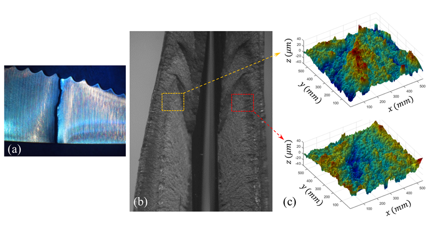
Figure 1: Association of forensic fragments. (a) Visual jigsaw match of the macroscopic crack trajectory. (b) Physical pattern match with comparative microscopy. (c) 3D representation of fracture surface, showing detailed topographic features at relevant scale.

can sometimes be used to recognize a “match” by an examiner or even by a layperson on a jury [5, 10]. However, experience, understanding, and judgment are needed by a forensic expert, to make reliable examination decisions using comparative microscopy and physical pattern match as indicated in Figure 1(b). Indeed, the microscopic details of the non-contiguous crack edges on the observation surface of Figure 1(a, b) cannot always be directly linked to a pair of fractured surfaces, except possibly by a highly experienced examiner. There are many published studies and case reports concerning fracture matching of different materials such as rubber shoe soles, wood, glass, tape, paper, skin, fishing line, cable, and, most commonly, metal [11, 12, 13, 14, 15, 16, 17, 18, 19, 20, 21, 22, 23, 24, 25, 26]. However, the microscopic details imprinted on the topological fracture surface of Figure 1(c) carry considerable information that could provide a quantitative forensic comparison with higher evidentiary value. Forensically, glass and metal fracture surfaces were shown to have highly stochastic fracture-branches due to the randomness of the microstructure and grain sizes [7, 27], with limited prior attempts to quantitatively match two measured fracture surface topologies [13, 9].

The rough and irregular metallic fracture surfaces carry many details of the metal microstructure and its loading history. Mandelbrot et al. [28] first showed the self-affine scaling properties of fractured surfaces to quantitatively correlate the material resistance to fracture with the resulting surface roughness. The self-affine nature of the fracture surface roughness has been experimentally verified for a wide range of materials and loading conditions. A key finding is the variation of such surface descriptors when measured parallel to the crack front and along the direction of propagation [29, 30, 31, 32]. Additionally, while self-affine characterization of the crack surface roughness exists at a length scale smaller than the fracture process scale (where stresses ahead of the crack tip reach critical value)  [33], the surface character becomes more complex and non-self-affine at larger length scales [34].

We first present an overview of the method and the study objectives. Then we describe the sample generation method and the imaging process used to create the data. We then provide a description of the statistical model which discriminates the matching fracture surfaces from the non-matching surfaces. We provide an evaluation of the method and several experiments to guide choices in imaging and in the parameters for the statistical model. Finally, we provide a discussion of the results and an illustration of how it would be applied in a forensic context. In the supplementary materials, we provide the underlying data, code to reproduce the analysis and figures, and additional information about the methods and materials. An R software package to perform the model fitting and analysis, MixMatrix, is available [35].

Method Overview and Study Objectives

Our objective is to find the scale of unique features on a fracture surface and then create a statistical method which uses the features to match them in a way which is suitable for use as evidence in court. Motivated by the observations about the self-affine nature of fracture surfaces, it can be speculated that a randomly propagating crack will exhibit unique fracture surface topological details when observed from a global coordinate that does not recognize the direction of crack propagation. This work explores the existence of such uniqueness of a randomly generated fracture surface at some relevant length scales. The uniqueness of these topological features implies that they can be used to individualize and distinguish the association of paired fracture surfaces. Our approach uses the fact that the microscopic features of the fracture surface in Figure 1(c) possess unique attributes at some relevant length scale that arise from the interaction of the propagating crack-tip process-zone and the microstructure details. The corresponding surface roughness analysis of this surface is shown in

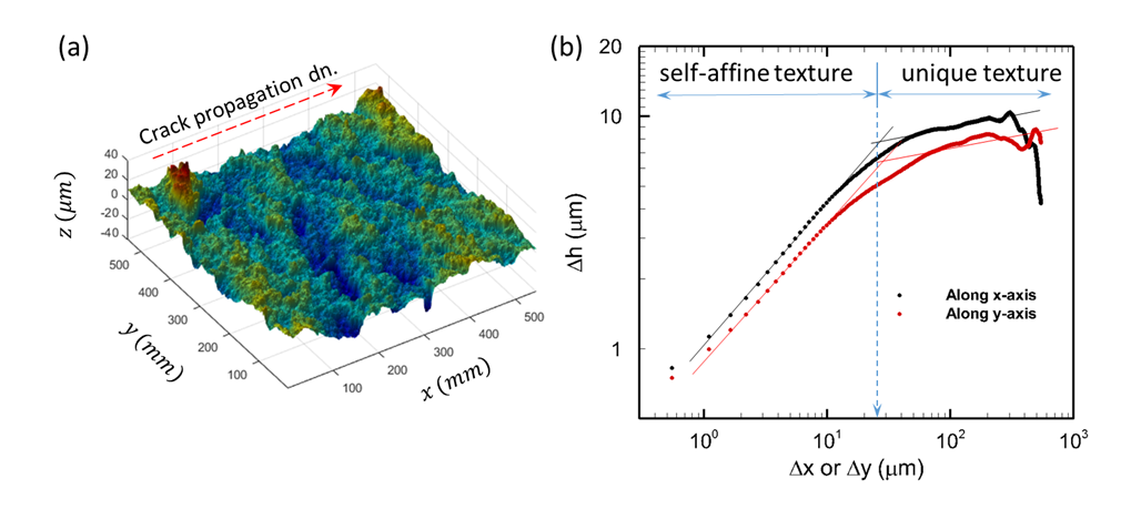
Figure 2: Fracture surface characteristics. (a) 3D surface topology rendering of fractured surface, showing a biased orientation of the low-frequency texture of the fracture surface. The direction of crack propagation is along the $x$-axis (b) Height-height correlation variation with the size of the imaging window, showing the domain of the self-affine deformation and the deviation of the fracture surface characteristics at higher length scales ($>100\mu m$), which could be used for matching purposes.

Figure 2 using a height-height correlation function, $\delta h(\delta\mathbf{x})=\sqrt{\langle[h(\mathbf{x}+\delta\mathbf{x})-h(\mathbf{x})]^{2}\rangle_{\mathbf{x}}}$, where $\langle\rangle$ denotes averaging over the $x$-direction. We see that at the small length scale of less than 10 – 20 $\mu m$, the roughness characteristic is self-affine (i.e. proportional to the analysis window scale). However, at larger length scales ($\approx 100\mu m$), this characteristic deviates, showing the individuality of the surface at that scale. These microscopic feature signatures exist on the entire fracture surface as it is influenced by three primary factors; namely the material microstructure, the intrinsic material resistance to fracture, and the direction of the applied load. This work explores the existence of such a length scale and the corresponding unique attributes of the fracture surface, as well as their applications to forensic comparison of fractured surfaces.

The height-height correlation function at this transition scale captures the uniqueness of the fracture surfaces, so we can use that function’s behavior in setting the observation scales for comparing matching and non-matching surfaces to produce a statistical model of each topological class’s behavior for use in classification. We can further combine multiple observations at different length scales or topological frequencies of a single surface into one model in order to improve the ability to discriminate between surfaces of the same class or materials and manufacturing processes (for instance, individualization of a pry tool from a similar batch of identical tools). The statistical model can produce a likelihood ratio or log-odds ratio of a new set of surfaces belonging to either class, which are common outputs of forensic matching methods [36, 37, 38, 39, 40, 41]. The creation of this model can also be used to estimate probabilities of misclassification and compare to the empirically observed rates of misclassification. Conceptually, this is similar to forensic matching models which are used in fingerprint identification and bullet matching. In fingerprint identification, features (minutiae) on the reference print and the latent print are marked and then the pair is given a score based on how well the two match, which may be part of a probabilistic model reporting a likelihood ratio or other probabilistic output [42]. The Congruent Matching Cells approach for matching breech face impressions on cartridge cases in ballistics takes a similar approach: it divides the scanned surfaces into cells and searches for matching cells on the other surface. It then uses this as an input to a statistical model which outputs a likelihood ratio [43, 44].

Materials and Methods

Sample Generation and Imaging

We consider two main material classes: sets of rectangular rods of a common tool steel material (SS-440C) and sets of knives from the same manufacturer fractured under control tension and bending configurations, respectively. The average grain size for both groups was approximately $dg$ = 25–35 $\mu m$. Four different sets of samples were established with nine specimens in the two sets of knives and ten specimens in the two sets of steel rods. Each knife specimen was fractured at random, in a manner similar to Figure 1(a).

For clarity, we refer to the surface attached to the knife handle as the base and the surface from the tip portion of the knife as the tip and apply the same terminology to samples from the rectangular steel rods. The microscopic features of pairs of fracture surfaces were analyzed by a standard non-contact 3D optical interferometer (Zygo-NewView 6300), which provides a height resolution of 20 $nm$ and spatial inter-point resolution of $0.45\mu m$ (Figure 2(a)) at an optical magnification of 20X. Surface height 3D topographic maps were acquired from the pairs of fracture surfaces, and quantized using Fourier transform based spectral analysis as summarized in Figure 3 in the image analysis step. Further details are given in the Supplement. The unique implementation of frequency space analysis provides a greater tolerance for the alignment of the pair of images. Further, it provides a straightforward segmentation of the surface topological frequency ranges for comparison.

The analysis first identified the scale of the significant features on each image pair and their distributions. It is established in fracture mechanics that the fracture process zone ahead of the crack tip typically extends to 2-3 times the grain size  [33], or around 50–75 $\mu m$ for the tested material system. This is the scale wherein the local stresses ahead of the crack tip reach a critical level, sufficient to overcome the intrinsic resistance of the material to fracture  [33]. Typically, a field of view (FOV) that covers at least 10 periods of the fracture process zone or about 20-30 grain diameters should be utilized to avert signal aliasing. An extended set of nine topological images with a $550\mu m$ FOV was collected on each fracture surface.

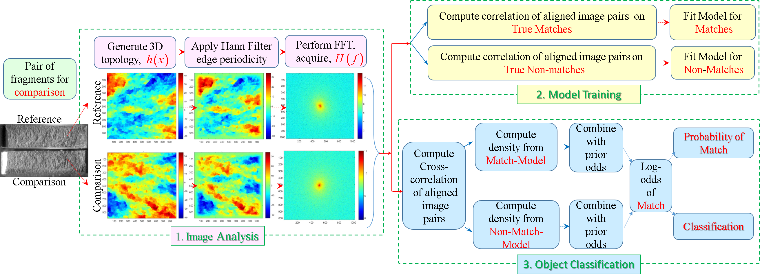
Figure 3: Flow chart showing the image analysis steps and model fitting/calibration step, followed by classification of new objects to provide classification probabilities. For a new field object, an examiner would use Step 1 to image the object and perform Step 3 using a model trained in Step 2 on samples of the same class to guide forensic conclusions.

Physical Matching by Spectral Analysis and Image Correlation

The measured height distribution function $h(\boldsymbol{x})$, defines the topology of the fracture surface at every spatial point, $\boldsymbol{x}$ on the fracture surface. Each wavelength on the fracture surface has a population, on the frequency domain $H(\boldsymbol{f})$, which is acquired using a Fast Fourier Transform (FFT) operator. For example, grain size has a distribution of frequencies across the spectrum rather than one specific frequency. Similarly, other microscopic fracture features would have a range of spectral distributions [45, 46]. For a pair of fractured surfaces, the population of these features contains relevant information about the physical processes present at each length-scale. After calculating the spectra of each pair of images, each spectrum was divided into multiple radial sectors. The segmented angular sectors for the frequency range ($0^{\circ}$, $180^{\circ}$) represents the entire data set, because the amplitude of $H(\boldsymbol{f})$ exhibits inversion symmetry. The spectral array size is proportional to $2^{n}$, as this is a mathematical feature of the FFT. For the image size employed in this work, a spectral array of 1024 by 1024 is acquired, although only the upper half is utilized because of symmetry. The radial segments for comparison on the frequency domain are chosen to reflect the physical process scales and the corresponding wavelength.

For comparison, we use the frequency amplitude, $\bar{H}(\boldsymbol{f})$ for each surface spectral frequency. To compare two surfaces, two-dimensional statistical correlations between their spectra are computed in banded radial frequencies, with increments in the bands determined by the scale of the image and the material microstructure, yielding a similarity measure on each frequency band for the corresponding pairs of images. To estimate the distribution for both the population of true matches and true non-matches, this is done for images from matching fracture surfaces and non-matching fracture surfaces as shown in Figure 4. On every fracture surface, a series of up to $k$-overlapping images were collected for the comparison process and the establishment of a statistical match. We used $k=9$ images with 75% overlap between successive images. The choice of overlap means there are three full independent sequential images on a surface.

The classification and matching process strategy is summarized in Figure 3, and is carried out in two steps; (a) Model training on an initial data set and (b) performing classification of new sample(s).

(a) Model Training/Fitting:

After determining which frequency bands are relevant for the comparison of fracture surfaces in a given material class, a model to distinguish matching from non-matching fracture surfaces can be developed. The behavior of the frequency band correlations in the population of matches and non-matches has to be estimated and modeled. The proposed framework provides a separate model for each class (i.e. match and non-match). The model training process is highlighted in Figure 3 and entails:

1. Choose a set of experimental fracture pairs to train the model.

2. Compute the correlations of the frequency bands for the sets of images for all matching and non-matching surface pairs.

3. Use the Fisher’s $z$ transformation on the correlation data to stabilize variance [47].

4. Fit models to describe the distribution of true matches and true non-matches, which account for the difference in location of the correlations and account for the covariance of the repeated observations across the surface.

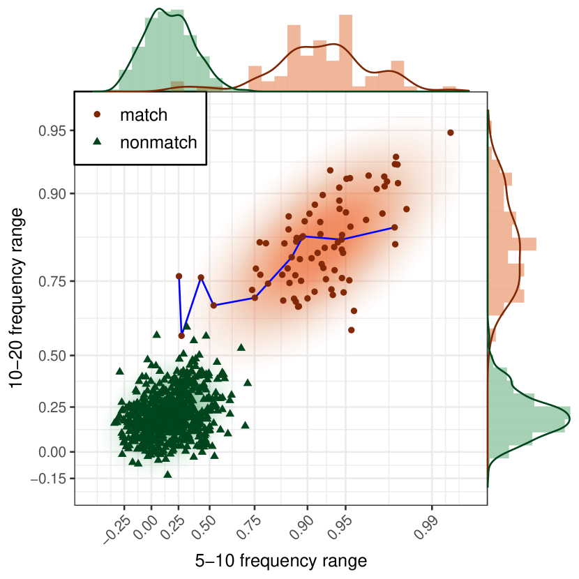
Figure 4: Scatter plot of correlations for 81 matched pairs and 648 non-matched pairs for the 5–10 and 10–20 $mm^{-1}$ frequency ranges on a Fisher-z (nonlinear) axis. The plot shows that true matches and true non-matches are distinguished in this example by features in the 5-10 and 10-20 $mm^{-1}$ frequency ranges. The connected points show the values of nine images from the same surface, indicating that while some individual images may not distinguish matches from non-matches, taking an ensemble of images from the surface helps perfectly discriminate the two classes.

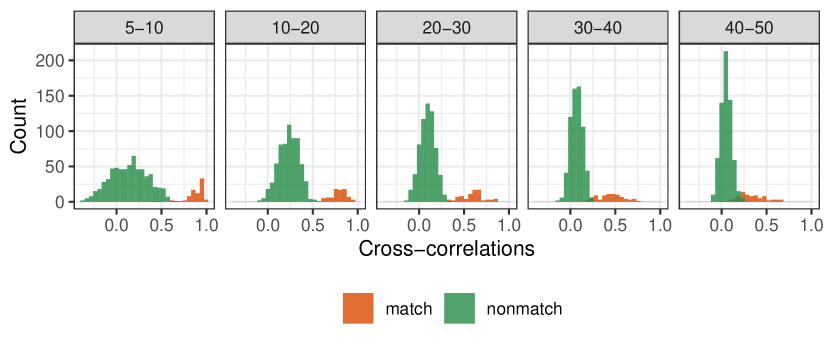
Figure 5: Histograms of correlations of true matches and true non-matches in one set of 9 surfaces with 9 images per surface split by frequency band. Lower frequencies are well-separated, but higher frequencies begin to have more substantial overlap.

Figure 4 illustrates the discrimination ability of the proposed method. The data in this illustration were derived from nine base-tip pairs from fractured knives. Nine images were taken from each base and tip fracture surface, resulting in 162 total images (81 from the tips and 81 from the bases). In this example, image pairs for when the tip and base surfaces were from the same knife are true matches (81 matched-pairs), while those pairs for which the tip and base surfaces were from different knives are true non-matches (648 unmatched-pairs). Correlation analysis showed clear separation (lower values for the true non-matches and higher values for the true matches) for the 5–10 and 10–20$mm^{-1}$ frequency-band range, as shown in Figure 5. At the lower frequency ranges, there is some overlap. Beyond these frequency ranges, the true match and the true non-match correlation distributions become less distinct and overlap more. In the set displayed in Figure 4, there is one image pair among the true matches which cannot be distinguished from the true non-matches and three other pairs that are ambiguous. To further improve the discrimination, considering multiple observations from the same surface would distinguish it from the non-matches, since the other observations on that surface are well-separated from the non-matches.

Because we have nine overlapping images for each specimen and two (or more) comparison frequencies, each comparison between two specimens provides a $2\times 9$ matrix of correlations. Accordingly, we propose using a matrix-variate distribution [48, 49] to model the densities of the matching and non-matching populations, and, specifically, a matrix-variate $t$ distribution (MxV$t$) because the data for the individual comparisons are approximately elliptically distributed but have heavier tails than a normal distribution. A definition of the distribution is in the supplement and the density is defined in Equation S-1 in the Supplement.

We use matrix-variate distributions to model the relationship between the two frequency bands in each image comparison and across the images being compared in the base and tip pair (e.g. Figure 4). Because of the overlapping-image structure of the data source, our model allows between-image correlations in the matrix-variate model to be related according to an autoregressive model of order 1 (or AR(1)) model (implying that immediately adjacent images can be correlated). We specify that the mean correlations in the two frequency bands remain the same across the images on a surface in the model. The fit of the model is estimated using an expectation-maximization (EM) algorithm developed for the matrix-variate $t$ distribution [50].

Classification of a new object

Suppose the fitted model has been trained on a set of $k$-images per fracture surface, yielding probability density functions $f_{1}$ corresponding to the population of true matches and $f_{2}$ corresponding to the population of true non-matches. Suppose also that there is a new pair of fracture surfaces that may or may not match. First, the correlations for the $k$-aligned image pairs in the chosen frequency bands are computed and transformed, yielding a new observation $X$, which is a matrix of observations of correlations with one row for each frequency band and one column for each pair of images—here, a $2\times k$ matrix. Then, presuming prior probability $p$ of being a true match and prior probability $1-p$ of being a true non-match, we can find, by combining prior probabilities and the match and non-match densities from the model, the posterior probability that the two surfaces match as follows:

$$P(X=match)=\frac{pf_{1}(X)}{pf_{1}(X)+(1-p)f_{2}(X)}$$

In the absence of prior information of the probability of a match, we are using an equal prior ($p=0.5$). A classification decision can then be made based on the posterior probability. The results can be expressed as a log-odds ratio. Changing the prior probabilities changes the log-odds ratio by adding a constant, so the specification of a prior at this point is unnecessary. If an equal prior is used, this expression can also be converted to a likelihood ratio (LR), which is a common method in forensic applications [36, 37, 38, 39, 40, 41], and these LR results can be incorporated into a framework for evaluating the strength of evidence under different sets of assumptions  [51]. Classification decisions can then be made under the rules of evidence relevant to the case. In this discussion, we will make classification decisions using a cutoff value of $0.5$.

Results and Discussion

Classification performance

There are two datasets from the knives and two from the steel bars: “K-1-1” is the first set of images from the first set of knives, and the imaging is independently repeated generating additional sets of images “K-1-2”and “K-1-3” for repeat analysis. “K-2” indicates the other set of knives, whereas “S-1” and “S-2” indicate the two steel bar samples. Figure 6 shows the classifications obtained by training on each of the four datasets, represented by one of the color boxes, with all 9 images per sample and classifying on all the sets of surfaces using the matrix-variate $t$ distribution and a common degrees of freedom parameter, $\nu=3,5,10,15,20$, and $30$. The output given in terms of the log-odds of being a match – log-odds larger than zero $(p=0.5)$ indicate classification as a match. While initially there are no false positives or false negatives, as the degrees of freedom parameter (DF or $\nu$) increases, there is one false positive, though this probability is very close to 0.5 and all of the true positives have a probability close to 1, which suggests using a classification threshold other than 0.5 would yield perfect classification. A different threshold can be chosen by selecting a low probability (such as $10^{-4}$) as a probability of false alarm and using the distribution of log-odds of the true non-matches to fix that threshold conservatively by selecting an upper confidence bound of that quantile [52]. Using the upper $95\%$ confidence bound for the threshold at which the false alarm probability based on the distribution of true negatives is $10^{-4}$ sets the threshold at a probability of 0.8375 for the most conservative training set at the setting of $\nu=10$, for example, which still results in perfect classification.

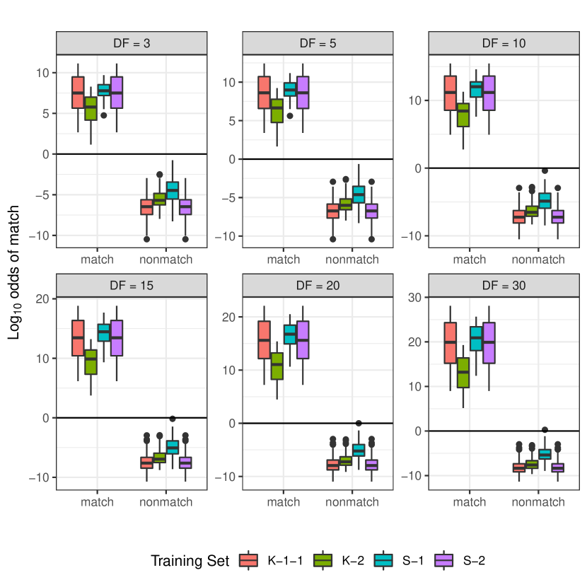
Figure 6: Log-odds of being a match split by training set and true class membership for matrix $t$ distributions with 3, 5, 10, 15, 20, and 30 degrees of freedom. Log-odds greater than 0 indicates greater odds of being a match than a non-match. The predictions for each training set are on all four sets of surfaces.

Reproducibility of results

In order to determine the reproducibility of results for a given sample, we re-imaged one of the knife samples three times and examined the distributions of the true match image correlations in Figure 7. The different re-imaged sets are labeled “K-1-1”, “K-1-2”, and “K-1-3”. The means of the distributions (indicated by the large shapes) are similar and the covariance matrices, visualized using 99% confidence ellipses, are also similar. Using the two-sample Peacock test, a two-dimensional extension of the Kolmogorov-Smirnov test [53, 54], there is no evidence these distributions differ ($p$-values: 1 and 2, $p=0.21$; 1 and 3, $p=0.32$; 2 and 3, $p=0.25$). We conclude, then, the imaging and analysis process are reproducible for the analyzed samples.

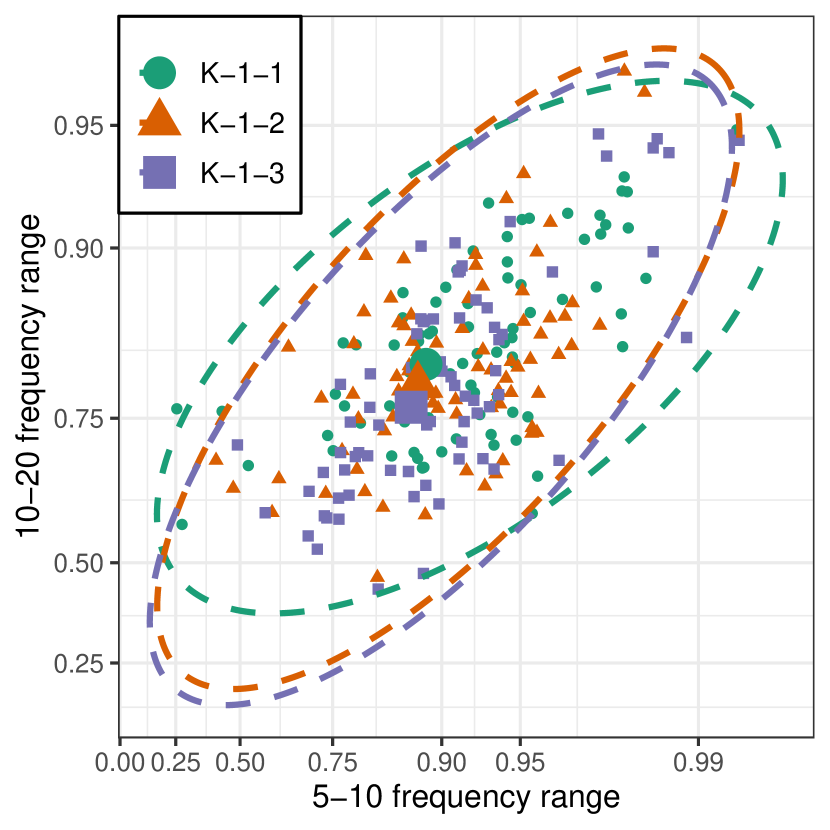
Figure 7: Individual true match correlations for three repetitions of images of the same set of 9 knives with 9 images per knife. This demonstrates that similar results will be obtained upon re-imaging the same surface, which is important in forensic applications. The large dots indicate the means of the sets and the ellipses are 99% tolerance ellipses, which provide a representation of the covariance matrices.

Selecting DF ($\nu$)

The training sets do not have a sufficient number of observations in both classes to estimate $\nu$ in the MxV$t$ model. However, the analysis in the previous section indicates it has some influence on the results. We performed a leave-one-out cross validation (LOOCV) procedure to provide guidance about the effects of changing the parameter. For each surface in a training set, a model was trained on the set of observations excluding that surface and tested on the observations using the excluded surface. This was done for $k=9$ images on training sets S-1 and S-2 and using $k=5$ images (restricting to the images with only 50% overlap) and $k=3$ images (restricting to the non-overlapping images) on all four training sets. The procedure was performed only on sets S-1 and S-2 for $k=9$ because nine surfaces are needed to fit the model and K-1-1 and K-2 have only nine surfaces, while S-1 and S-2 have ten. Figure 8 shows the results for $k=3$, $5$, and $9$ respectively. The parameter $\nu$ varied from $3$ to $30$. In all cases, the true matches and true non-matches were perfectly classified using a threshold probability of $0.5$ (log-odds of $0$). Higher values of $\nu$ had more separation between the classes. Using 9 images with 75% overlap had greater separation than 5 images with 50% overlap and greater separation between the identification of true matches. However, given that there is perfect classification in all cases, this does not provide much guidance on the selection of $\nu$.

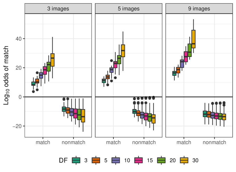
Figure 8: Cross-validation results for models fit using $k=3$, $5$, and $9$ images of each surface. The cross-validation was done to provide guidance about the number of images and the choice of DF ($\nu$). There were no false positives or false negatives in this analysis, so it did not provide any conclusive results.

Number of images needed for discrimination and model selection

Due to unique topological disturbance in some images (e.g. grains fall out from the fracture surface or significantly large out of plane curvature within the range of comparisons), there is not perfect separation between all image pairs for the matches and non-matches. This can be noticed on Figure 7 where some image pairs have a correlation coefficient of less than 0.50 for the two bands of frequency analysis. To mitigate the influence of local topological disturbances when deciding whether a pair of fragments represent a match or not, multiple observations are needed. To determine how many images are needed to optimize classification performance, we started by training models using all nine images on each training set as before. We again used the MxV$t$ model with $\nu=3,5,10,15,20$, and $30$,

and then tested them on subsets of consecutive images of size $k$, for $k=2,3,\ldots 9$ with the model reduced to considering only the selected images. A summary of the complete results are given in the Supplement.

In Figure 9, models with higher $\nu$ have higher false negative rates for all values of $k$. For values of $k$ over 4, only $20$ and $30$ DF have false negatives. Low values of the degrees of freedom parameter have false positives. All of this suggests that choosing a value near $\nu=10$ and $k\geq 5$ images are sufficient for optimal classification. Figure 10 displays complete results for a model with 10 DF. As $k$ increases, the typical classification results become more separated. However, even with only two images considered in the test cases for the 10 DF model, the accuracy is very high and the worst case of a false positive is classified with only a probability of 0.921 and the worst case of a false negative is classified with a probability of 0.504.

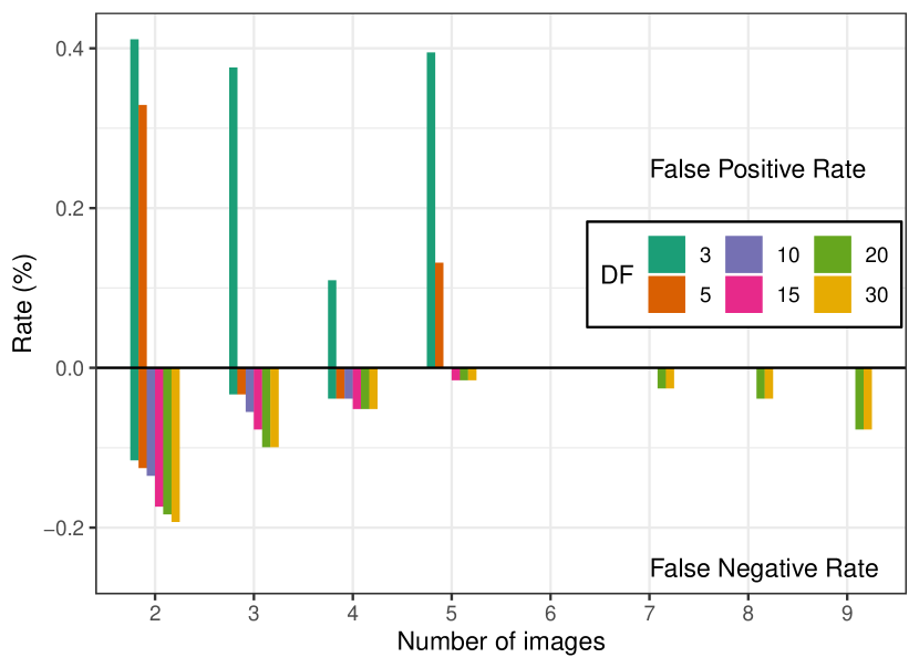
Figure 9: Rates of false positive and false negative classifications (in %) using models trained on the four different sets of surfaces and tested on consecutive subsets of those images for $k=2,3,\ldots,9$.

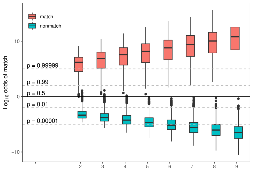
Figure 10: Distributions of the log-odds of a match using models trained on the four different sets of surfaces and tested on subsets of $k$ consecutive images for $k=2,3,\ldots,9$ for a model with 10 degrees of freedom.

Amount of overlap

Guided by the results of Figure 10, it is apparent that we need at least 5 to 6 images for adequate discrimination. We reassessed the imaging procedure to gauge the role of the image-overlap ratio. The initial experiment involved imaging surfaces using nine images with 75% overlap between images, which provides three observations for each point on the surface, apart from the edges. However, a similar area can be imaged using 5 images with 50% overlap, which produces two observations of each point on the surface apart from the edges, or using 3 non-overlapping images, which raises the question of whether anything is gained by having an additional third image of the same area and, if so, what level of overlap is optimal.

We can evaluate this by providing an analysis similar to that done previously: looking at the classification results when restricted to cases with the specified overlap. We train classifiers on the same sets as before, except using 5 images with 50% overlap instead of 9 images with 75% overlap and then test the models by classifying pairs of surfaces using all possible subsets of those images on the surface of sizes 2, 3, 4, and 5. When restricted to the case of 50% overlap, there is only perfect classification when all five images are included and the degrees of freedom ($\nu$) are less than 20 (Figure 11). In all cases, there are no false negatives.

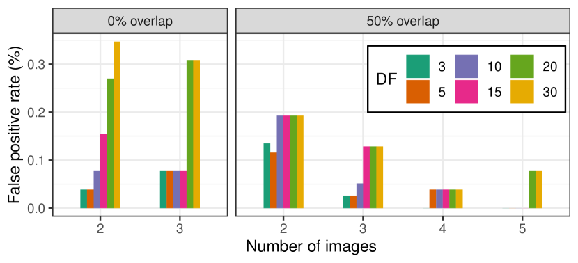
Figure 11: Rates of false positive classifications (in %) using models trained on the four different sets of surfaces using only the images with at most 50% overlap and tested on subsets of $k$ consecutive images for $k=2,3,4,5$ and using only the 3 non-overlapping images and tested on subsets of $k$ consecutive images for $k=2,3$.

We perform a similar exercise in the case of the non-overlapping images. There are three non-overlapping images per surface which can be used to train classifiers and the models can then be tested on subsets of those images on each surface of sizes 2 and 3. In the case of non-overlapping images, none of the models results in perfect classification. The false positives for each model are also shown in Figure 11. There are no false negatives in the classification decisions.

This suggests that, while having more images is generally better, using 5 images with 50% overlap appears to be sufficient if all the images are used. Imaging the entire surface with 50% overlap outperforms imaging the entire surface with 75% overlap in the sense that it works for all of the classes of model. However, if training with 9 images with 75% overlap is possible, testing on new surfaces is feasible with as few as 5 test images with an appropriate choice of the degrees of freedom parameter in the model.

Conclusions

This paper provides a formal quantitative basis for matching metal fragments found at crime scenes. Our novel approach combines fracture mechanics with statistics and machine learning to quantify the probability that two candidate specimens are a match. Our methodology utilizes 3D spectral analysis of the fracture surface topography, mapped by white light non-contact surface profilometers. Specifically, our framework realizes the unique attributes of fracture surfaces at a length scale defined by the fracture process zone, and uses them to do a quantitative physical match analysis of metal fragments. Fracture surface morphology has been analyzed for many classes of materials and shown to be self-affine within a scale relevant to the microscopic scale of the fracture process. We exploit these unique features to quantitatively distinguish the microscopic features on fracture surfaces. Statistical learning tools are used to classify specimens.

Using at least 5-6 images in the case of 75% image overlap or five images with 50% image overlap, we found that the matrix-variate t-distribution with 10-15 degrees of freedom, and a first-order autoregressive correlation structure to describe between-image correlation provides highly-effective discrimination between matching and non-matching surface pairs. Our results show the unique individuality of a pair of fractured surfaces at wavelengths in the range of $2-8$ grain diameters ($50-200\mu m$, or the frequency range of $5-20mm^{-1}$ for examined tool-steel). Near-perfect discrimination was achieved, even when the quality of some of the image pairs deteriorated. Such low-quality images arise from high topological details with a large aspect ratio that might shadow the surrounding details, and might disturb one of the frequency bands. Despite these difficulties, our statistical methods using two frequency bands and an extended number of base-tip image pairs yielded highly-accurate match decisions. Among the broad range of training sample sets, this domain of unique individuality was found to be persistent and easily identified. Our results provide a method for performing matching of fragments with recommendations for model parameters, procedures for training models on a similar class of materials with the same grain sizes, and procedures for testing new samples. Repeated imaging on the same surfaces consistently provided similar results. Our framework provided near-perfect matching with high confidence and so has the potential to be of significant impact, providing the ability to introduce more formality into how forensic match comparisons are conducted, through a rigorous mathematical framework. Our framework is also general enough to be applied, after suitable modifications, to a broad range of fractured materials and/or toolmarks, with diverse textures and mechanical properties. In doing so, we expect our novel methodology and findings to help forensic scientists and practitioners place forensic decision-making on a firmer scientific footing. This can help formalize the scientific basis for conclusive matching of fragments leading to quantitative and more objective forensic decisions.

Supplementary Materials

-A Details on Sample Generation and Imaging

Two main material classes are considered: two sets of nine single serrated edged knives from the same manufacturer (Chicago Cutlery), and two sets of ten rectangular (0.25" wide, and 1/16" thick) rods of a common tool steel material (SS-440C) cut from the same metal sheet to minimize any variability from the manufacturer. The knives were fractured at random using a controlled bend fixture shown in Figure 12(a). a set of fractured pairs of knives is shown in Figure 12(b). The two sets of the tool steel were loaded under either controlled tensile loading at 1 mm/ min displacement rate (Figure 13(a)) or controlled bending loading at 1.5 $mm/min$ displacement rate (Figure 13(c)) until fracture. The pairs of tool steel samples fractured by tension and bending are shown in Figure 12(b,d), respectively. The average grain size for both groups was approximately $dg$ = 25–35 $\mu m$. For clarity, we refer to the surface attached to the knife handle as the base and the surface from the top portion of the knife as the tip. The same terminology was applied to the tool steel samples as well. The microscopic features of pairs of fracture surfaces were aligned and analyzed by a standard non-contact 3D optical interferometer (Zygo-NewView 6300), which provides a height resolution of 20 $nm$ and spatial inter-point resolution of 0.45$\mu m$ (Figure 2(a)). Surface height 3D topographic maps were acquired from the pairs of fracture surfaces and quantized using spectral analysis, as summarized in Figure 3. An extended set of nine topological images with a 550 $\mu m$ field of view were collected on each fracture surface, provides a mapping of 0.55 $\mu m/pixel$ is shown in Figure 14. For the collected set of images, digital filters for surface tilt correction and spike noise removal were applied.

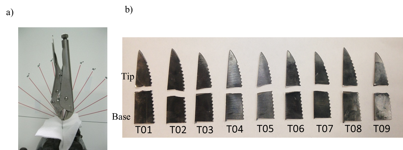
Figure 12: Knife-breaking protocol. (a) Loading fixture. (b) Pairs of knives from the same manufacturer fractured by bending.

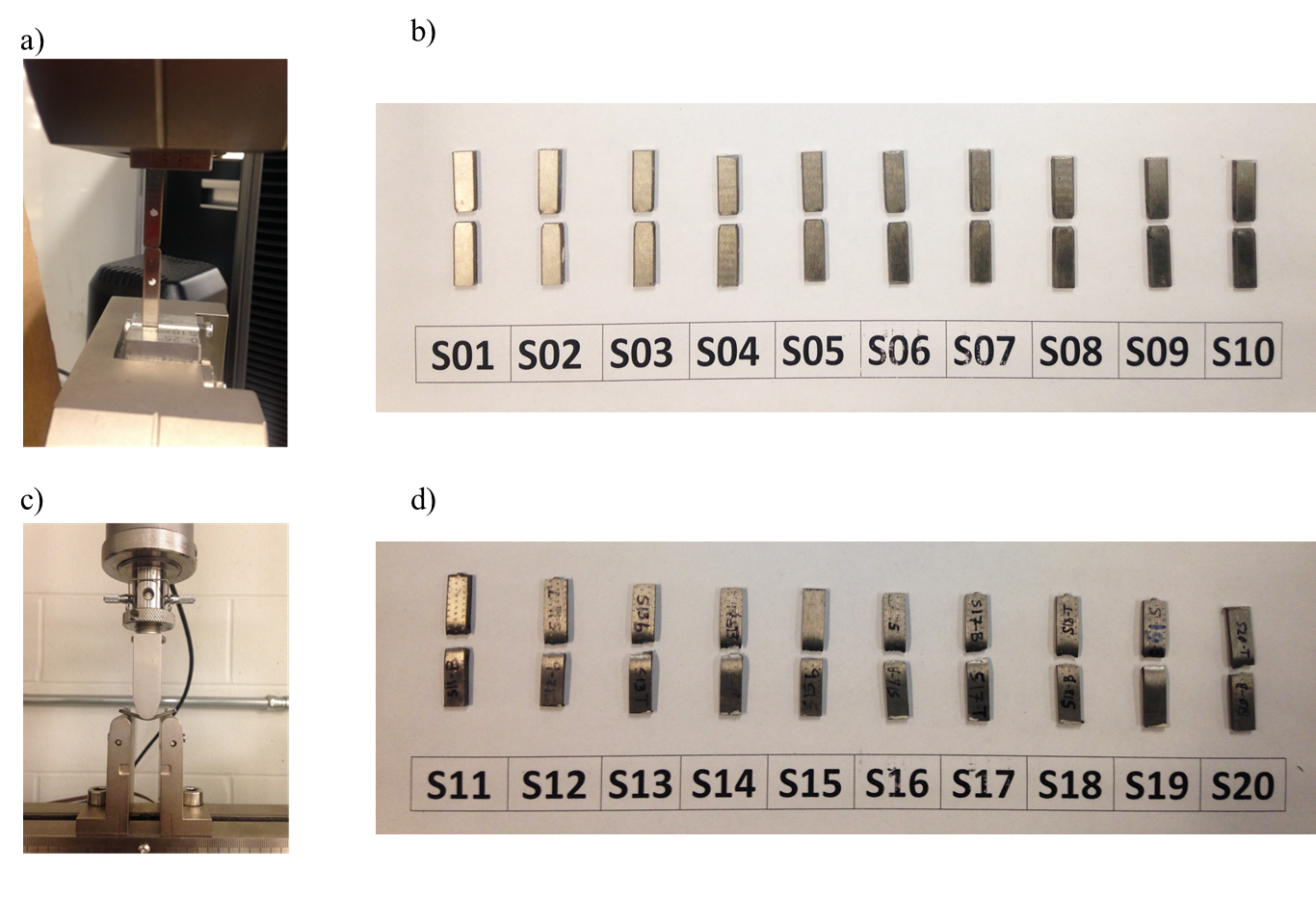
Figure 13: Sample generation protocol. (a) sample fracture under a controlled tensile loading, (b) pairs of steel samples fractured by tensile loading, (c) sample fracture under three point bending loading, (d) pairs of steel samples fractured under bending.

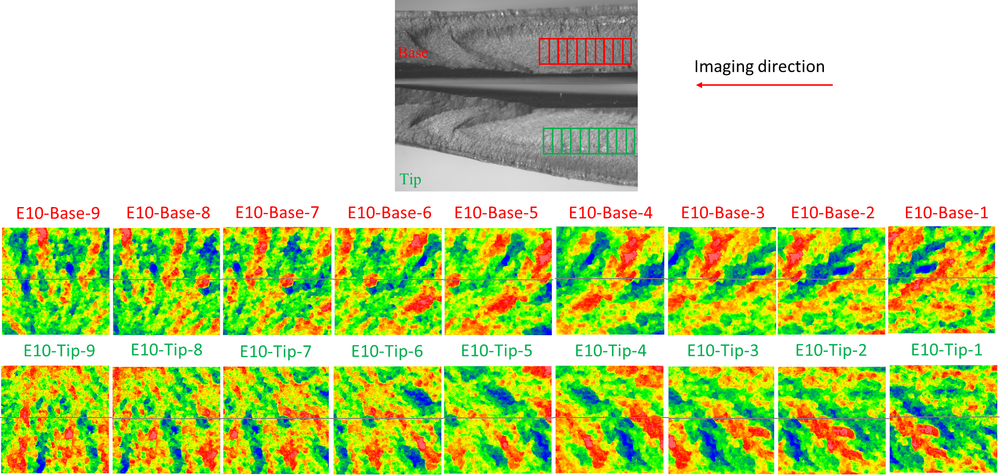
Figure 14: Nine overlapped and aligned images from a pair of fracture surfaces.

-B Matrix Variate Normal and Matrix Variate t Distributions

The matrix variate normal distribution is related to the matrix variate $t$ distribution and is used to construct it. In this section, we define these distributions as used in the paper.

Definition 1.

A random $p\times q$ (in this example, $p=2$ and $q=9$) matrix $\boldsymbol{X}$ has a matrix-variate normal distribution with parameters $(\mathbf{M},\boldsymbol{\Sigma},\boldsymbol{\Omega}$), with $\mathbf{M}$ a $p\times q$ matrix specifying the mean, $\boldsymbol{\Sigma}$ a $p\times p$ covariance matrix defining the relationship between the rows, $\boldsymbol{\Omega}$ a $q\times q$ covariance matrix defining the relationship between the columns, if it has the probability density function (PDF)

$$f(\boldsymbol{X};\mathbf{M},\boldsymbol{\Sigma},\boldsymbol{\Omega}) =\frac{\exp\left(-\frac{1}{2}\,\mathrm{tr}\left[\boldsymbol{\Omega}^{-1}(\boldsymbol{X}-\mathbf{M})^{T}\boldsymbol{\Sigma}^{-1}(\boldsymbol{X}-\mathbf{M})\right]\right)}{(2\pi)^{pq/2}|\boldsymbol{\Omega}|^{p/2}|\boldsymbol{\Sigma}|^{q/2}},$$

where $|\cdot|$ denotes the determinant, $\mathbf{M}$ is a $p\times q$ matrix that is the mean of $\boldsymbol{X}$, and $\boldsymbol{\Sigma}$ and $\boldsymbol{\Omega}>0$ describing the covariances between, respectively, each of the $p$ rows and the $q$ columns of $\boldsymbol{X}$. We write $\boldsymbol{X}\sim\mathcal{N}_{p,q}(\mathbf{M},\boldsymbol{\Sigma},\boldsymbol{\Omega})$. For identifiability, we set the first element of $\boldsymbol{\Sigma}$ to be unity.

The matrix variate normal distribution can be considered, after rearranging into a vector (denoted by vec($\boldsymbol{X}$)), to be from a multivariate normal (MVN) distribution with a Kronecker product covariance structure [55]. So, if $\boldsymbol{X}\sim\mathcal{N}_{p,q}(\mathbf{M},\boldsymbol{\Sigma},\boldsymbol{\Omega})$, then $\mathrm{vec}(\boldsymbol{X})\sim\mathcal{N}_{pq}(\mathrm{vec}(\mathbf{M}),\boldsymbol{\Omega}\otimes\boldsymbol{\Sigma}).$

In the case of over-dispersion, that is, higher variance than can be explained by a normal model, it may be appropriate to use a distribution with fatter tails, such as a $t$ distribution. A matrix variate $t$ distribution, here abbreviated as MxV$t$, can be defined as follows:

Definition 2.

A random $p\times q$ matrix $\boldsymbol{X}$ has a MxV$t$ distribution with parameters $(\mathbf{M},\boldsymbol{\Sigma},\boldsymbol{\Omega}$) of similar order as in Definition 1 (with $\boldsymbol{\Sigma}$ and $\boldsymbol{\Omega}>0$) and degrees of freedom (df) $\nu\geq 1$ if its PDF is

$$f(\boldsymbol{X};\nu,\mathbf{M},\boldsymbol{\Sigma},\boldsymbol{\Omega})={\frac{\Gamma_{p}\left({\frac{\nu+p+q-1}{2}}\right)}{(\pi)^{{\frac{pq}{2}}}\Gamma_{p}\left({\frac{\nu+p-1}{2}}\right)}}|\boldsymbol{\Omega}|^{{-{\frac{p}{2}}}}|\boldsymbol{\Sigma}|^{{-{\frac{q}{2}}}}\left|{\mathbf{I}}_{p}+\boldsymbol{\Sigma}^{{-1}}(\boldsymbol{X}-{\mathbf{M}})\boldsymbol{\Omega}^{{-1}}(\boldsymbol{X}-{\mathbf{M}})^{{{\rm{T}}}}\right|^{{-{\frac{\nu+p+q-1}{2}}}}.$$ (S1)

We use the notation $\boldsymbol{X}\sim t_{p,q}(\nu,\mathbf{M},\boldsymbol{\Sigma},\boldsymbol{\Omega})$ to indicate that $\boldsymbol{X}$ has this density.

We mention some properties of the MxV$t$ distribution relevant to this paper.

1. For $p=1$ and $\boldsymbol{\Sigma}\equiv\nu$ (or $q=1$ and $\boldsymbol{\Omega}\equiv\nu$), the MxV$t$ distribution reduces to its vector-multivariate $t$ (MVT) cousin.

2. Let the random matrix $\boldsymbol{S}\sim{\mathcal{W}}_{p}(\nu+p-1,\boldsymbol{\Sigma}^{-1})$, where ${\mathcal{W}}_{p}(\kappa,\boldsymbol{\Psi})$ is the $p\times p$-dimensional Wishart distribution with d.f. $\kappa$ and scale matrix $\boldsymbol{\Psi}$. If $\boldsymbol{X}\mid\boldsymbol{S}\sim{\mathcal{N}}_{p,q}(\mathbf{M},\boldsymbol{S}^{-1},\boldsymbol{\Omega})$, then $\boldsymbol{X}\sim t_{p,q}(\nu,\mathbf{M},\boldsymbol{\Sigma},\boldsymbol{\Omega})$ (see [55], page 135). Further, $\boldsymbol{S}\mid\boldsymbol{X}\sim{\mathcal{W}}_{p}(\nu+p+q-1,[(\boldsymbol{X}-\mathbf{M})\boldsymbol{\Omega}^{-1}(\boldsymbol{X}-\mathbf{M})^{T}+\boldsymbol{\Sigma}]^{-1})$ [49].

As $\nu\to\infty$, the MxV$t$ converges to a matrix variate normal distribution. In this application, the correlations between individual images are taken to be identically distributed within each class (true matches and true non-matches), which implies for each class the $\mathbf{M}$ matrix is constant along its rows and that the $\boldsymbol{\Omega}$ matrix can be expressed as a correlation matrix with a unit diagonal. We further assume that the covariance of the observations between neighbors remain the same across the imaged surface (e.g., the relationship between the first and second images is the same as the relationship between the eighth and ninth images). Because of the overlapping structure, we use an autoregressive covariance structure to describe the covariance and use an AR(1) model in this application. In an AR(1) correlation matrix, the correlation of any two adjacent elements is $\rho$ and for two elements, $a_{i}$ and $a_{j}$, the correlation between them is $\rho^{|i-j|}$, with $|\rho|<1$.

-C Tables of Results

Each table contains classification results for different settings of the $\nu$ parameter and $k$ parameter. Four different data sets were used as training sets: two sets with 9 samples and 9 images per sample (with 75% overlap) and two sets with 10 samples and 9 images per sample (with 75% overlap). The sets with 9 samples, then, had 81 sets of comparisons between base and tip: 9 true matches and 72 true non-matches. The sets with 10 samples had 100 sets of comparisons between base and tip: 10 true matches and 90 true non-matches. In the first table, all 9 images (with 75% overlap) for every surface are included in the model training. In the second table, only 5 images with 50% overlap are included in the model training. In the final table, only 3 non-overlapping images are included. For each setting of $\nu$ and for each of the four different datasets, we train a model and then test on all four datasets by classifying all consecutive subsets of images of size $k$. In the tables, the first two columns indicate the value of $\nu$ and the number of consecutive images, $k$, used to classify test samples. The final two columns tally how many were truly matching or truly non-matching comparisons. All models used equal priors and a classification threshold of 0 log-odds (equivalent to a posterior probability of 0.5).

To compute the False Positive Rate (FPR) for any row, divide the number in the False Pos column by the number of True Non-Matches (equivalently, by the sum of False Pos and True Neg columns). Other statistics can be computed in a similar manner for each row.

TABLE I: Summary of match and non-match decisions for the models fitted using all 9 images and tested on all consecutive subsets of images of size $k$.

Model	k	False Pos	False Neg	True Pos	True Neg	True Match	True Non-Match
$\nu$ = 3	2	12	5	1211	10356	1216	10368
$\nu$ = 3	3	3	4	1060	9069	1064	9072
$\nu$ = 3	4	3	1	911	7773	912	7776
$\nu$ = 3	5	0	3	757	6480	760	6480
$\nu$ = 3	6	0	0	608	5184	608	5184
$\nu$ = 3	7	0	0	456	3888	456	3888
$\nu$ = 3	8	0	0	304	2592	304	2592
$\nu$ = 3	9	0	0	152	1296	152	1296
$\nu$ = 5	2	13	4	1212	10355	1216	10368
$\nu$ = 5	3	3	0	1064	9069	1064	9072
$\nu$ = 5	4	3	0	912	7773	912	7776
$\nu$ = 5	5	0	1	759	6480	760	6480
$\nu$ = 5	6	0	0	608	5184	608	5184
$\nu$ = 5	7	0	0	456	3888	456	3888
$\nu$ = 5	8	0	0	304	2592	304	2592
$\nu$ = 5	9	0	0	152	1296	152	1296
$\nu$ = 10	2	14	0	1216	10354	1216	10368
$\nu$ = 10	3	5	0	1064	9067	1064	9072
$\nu$ = 10	4	3	0	912	7773	912	7776
$\nu$ = 10	5	0	0	760	6480	760	6480
$\nu$ = 10	6	0	0	608	5184	608	5184
$\nu$ = 10	7	0	0	456	3888	456	3888
$\nu$ = 10	8	0	0	304	2592	304	2592
$\nu$ = 10	9	0	0	152	1296	152	1296
$\nu$ = 15	2	18	0	1216	10350	1216	10368
$\nu$ = 15	3	7	0	1064	9065	1064	9072
$\nu$ = 15	4	4	0	912	7772	912	7776
$\nu$ = 15	5	1	0	760	6479	760	6480
$\nu$ = 15	6	0	0	608	5184	608	5184
$\nu$ = 15	7	0	0	456	3888	456	3888
$\nu$ = 15	8	0	0	304	2592	304	2592
$\nu$ = 15	9	0	0	152	1296	152	1296
$\nu$ = 20	2	19	0	1216	10349	1216	10368
$\nu$ = 20	3	9	0	1064	9063	1064	9072
$\nu$ = 20	4	4	0	912	7772	912	7776
$\nu$ = 20	5	1	0	760	6479	760	6480
$\nu$ = 20	6	0	0	608	5184	608	5184
$\nu$ = 20	7	1	0	456	3887	456	3888
$\nu$ = 20	8	1	0	304	2591	304	2592
$\nu$ = 20	9	1	0	152	1295	152	1296
$\nu$ = 30	2	20	0	1216	10348	1216	10368
$\nu$ = 30	3	9	0	1064	9063	1064	9072
$\nu$ = 30	4	4	0	912	7772	912	7776
$\nu$ = 30	5	1	0	760	6479	760	6480
$\nu$ = 30	6	0	0	608	5184	608	5184
$\nu$ = 30	7	1	0	456	3887	456	3888
$\nu$ = 30	8	1	0	304	2591	304	2592
$\nu$ = 30	9	1	0	152	1295	152	1296

TABLE II: Summary of match and non-match decisions for the models fitted using 5 images with at most 50% overlap and tested on all consecutive subsets of images of size $k$.

Model	k	False Pos	False Neg	True Pos	True Neg	True Match	True Non-Match
$\nu$ = 3	2	7	0	608	5177	608	5184
$\nu$ = 3	3	1	0	456	3887	456	3888
$\nu$ = 3	4	0	0	304	2592	304	2592
$\nu$ = 3	5	0	0	152	1296	152	1296
$\nu$ = 5	2	6	0	608	5178	608	5184
$\nu$ = 5	3	1	0	456	3887	456	3888
$\nu$ = 5	4	1	0	304	2591	304	2592
$\nu$ = 5	5	0	0	152	1296	152	1296
$\nu$ = 10	2	10	0	608	5174	608	5184
$\nu$ = 10	3	2	0	456	3886	456	3888
$\nu$ = 10	4	1	0	304	2591	304	2592
$\nu$ = 10	5	0	0	152	1296	152	1296
$\nu$ = 15	2	10	0	608	5174	608	5184
$\nu$ = 15	3	5	0	456	3883	456	3888
$\nu$ = 15	4	1	0	304	2591	304	2592
$\nu$ = 15	5	0	0	152	1296	152	1296
$\nu$ = 20	2	10	0	608	5174	608	5184
$\nu$ = 20	3	5	0	456	3883	456	3888
$\nu$ = 20	4	1	0	304	2591	304	2592
$\nu$ = 20	5	1	0	152	1295	152	1296
$\nu$ = 30	2	10	0	608	5174	608	5184
$\nu$ = 30	3	5	0	456	3883	456	3888
$\nu$ = 30	4	1	0	304	2591	304	2592
$\nu$ = 30	5	1	0	152	1295	152	1296

TABLE III: Summary of match and non-match decisions for the models fitted using 3 adjacent non-overlapping images and tested on all consecutive subsets of images of size $k$.

Model	k	False Pos	False Neg	True Pos	True Neg	True Match	True Non-Match
$\nu$ = 3	2	1	0	304	2591	304	2592
$\nu$ = 3	3	1	0	152	1295	152	1296
$\nu$ = 5	2	1	0	304	2591	304	2592
$\nu$ = 5	3	1	0	152	1295	152	1296
$\nu$ = 10	2	2	0	304	2590	304	2592
$\nu$ = 10	3	1	0	152	1295	152	1296
$\nu$ = 15	2	4	0	304	2588	304	2592
$\nu$ = 15	3	1	0	152	1295	152	1296
$\nu$ = 20	2	7	0	304	2585	304	2592
$\nu$ = 20	3	4	0	152	1292	152	1296
$\nu$ = 30	2	9	0	304	2583	304	2592
$\nu$ = 30	3	4	0	152	1292	152	1296

References

- [1] H. O. Fradella and A. L. Fogary, “The impact of Daubert on forensic science,” Pepperdine Law Review, vol. 31, p. 323, 2003–2004.
- [2] N. R. Council, Strengthening Forensic Science in the United States: A Path Forward. Washington, DC: The National Academies Press, 2009. [Online]. Available: https://www.nap.edu/catalog/12589/strengthening-forensic-science-in-the-united-states-a-path-forward
- [3] J. Almirall, H. Arkes, J. Lentini, F. Mowrer, and J. Pawliszyn, Forensic science assessments: a quality and gap analysis–fire examination. Washington, DC: American Association for the Advancement of Science, 2017.
- [4] W. Thompson, J. Black, A. Jain, and J. Kadane, Forensic science assessments: a quality and gap analysis–latent fingerprint examination. Washington, DC: American Association for the Advancement of Science, 2017.
- [5] J. Vanderkolk, Forensic Comparative Science: Qualitative Quantitative Source Determination of Unique Impressions, Images, and Objects. Cambridge, MA: Academic Press, jul 2009. [Online]. Available: https://www.xarg.org/ref/a/B074CCCQJC/
- [6] T. Van Dijk and P. Sheldon, The Practice Of Crime Scene Investigation (International Forensic Science and Investigation Book 10). Boca Raton, Florida: CRC Press, apr 2004. [Online]. Available: https://www.xarg.org/ref/a/B00UVAK1NA/
- [7] H. W. Katterwe, “Fracture matching and repetitive experiments: a contribution of validation,” AFTE JOURNAL, vol. 37, no. 3, p. 229, 2005.
- [8] J. Miller and H. Kong, “Metal fractures: Matching and non-matching patterns,” AFTE Journal, vol. 38, no. 2, pp. 133–165, 2006.
- [9] L. K. Claytor and A. L. Davis, “A validation of fracture matching through the microscopic examination of the fractured surfaces of hacksaw blades,” AFTE JOURNAL, vol. 42, no. 4, p. 323, 2010.
- [10] T. Van Dijk and P. Sheldon, “Physical comparative evidence,” in The Practice Of Crime Scene Investigation. CRC Press, 2004, pp. 393–418.
- [11] A. Klein, L. Nedivi, and H. Silverwater, “Physical match of fragmented bullets,” Journal of Forensic Science, vol. 45, no. 3, pp. 722–727, May 2000.
- [12] K. Walsh, T. Gummer, and J. Buckleton, “Matching vehicle parts back to the vehicle,” AFTE Journal, vol. 26, no. 4, pp. 287–289, October 1994.
- [13] V. R. Matricardi, M. S. Clarke, and F. S. DeRonja, “The comparison of broken surfaces: A scanning electron micrscopic study,” Journal of Forensic Science, vol. 20, no. 3, pp. 507–523, May 1975.
- [14] E. A. McKinstry, “Fracture match – a case study,” AFTE Journal, vol. 30, no. 2, pp. 343–344, Spring 1998.
- [15] D. J. Verbeke, “An indirect identification,” AFTE Journal, vol. 7, no. 1, pp. 18–19, March 1975.
- [16] D. Townshend, “Identification of fracture marks,” AFTE Journal, vol. 8, no. 2, pp. 74–75, July 1976.
- [17] D. J. Dillon, “Comparisons of extrusion striae to individualize evidence,” AFTE Journal, vol. 8, no. 2, pp. 69–70, July 1976.
- [18] G. Karim, “A pattern-fit identification of severed exhaust tailpipe sections in a homicide case,” AFTE Journal, vol. 36, no. 1, pp. 65–66, Winter 2004.
- [19] E. D. Smith, “Bullet and fragment identified through impression mark,” AFTE Journal, vol. 36, no. 3, p. 243, Summer 2004.
- [20] H. Katterwe, R. Goebel, and K. D. Gross, “The comparison scanning electron microscope within the field of forensic science,” AFTE Journal, vol. 15, no. 3, pp. 141–146, July 1983.
- [21] R. Goebel, K. D. Gross, H. Katterwe, and W. Kammrath, “The comparison scanning electron microscope: First experiments in forensic application,” AFTE Journal, vol. 15, no. 2, pp. 47–55, April 1983.
- [22] B. Moran, “Physical match/toolmark identification involving rubber shoe sole fragments,” AFTE Journal, vol. 16, no. 3, pp. 126–128, July 1984.
- [23] D. Rawls, “A rare identification of glass,” AFTE Journal, vol. 20, no. 2, pp. 154–156, April 1988.
- [24] R. A. Hathaway, “Physical wood match of a broken pool cue stick,” AFTE Journal, vol. 26, no. 3, pp. 185–186, July 1994.
- [25] X. Zheng, J. Soons, T. V. Vorburger, J. Song, T. Renegar, and R. Thompson, “Applications of surface metrology in firearm identification,” Surface Topography: Metrology and Properties, vol. 2, no. 1, p. 014012, jan 2014. [Online]. Available: https://doi.org/10.1088%2F2051-672x%2F2%2F1%2F014012
- [26] N. D. K. Petraco, P. Shenkin, J. Speir, P. Diaczuk, P. A. Pizzola, C. Gambino, and N. Petraco, “Addressing the national academy of sciences’ challenge: a method for statistical pattern comparison of striated tool marks,” Journal of Forensic Sciences, vol. 57, no. 4, pp. 900–911, 2012. [Online]. Available: https://doi.org/10.1111/j.1556-4029.2012.02115.x
- [27] H. Katterwe, R. Goebel, and K. Grooss, “The comparison scanning electron microscope within the field of forensic science.” Scanning Electron Microscopy, vol. 1982, no. Pt 2, pp. 499–504, 1982.
- [28] B. B. Mandelbrot, D. E. Passoja, and A. J. Paullay, “Fractal character of fracture surfaces of metals,” Nature, vol. 308, no. 5961, pp. 721–722, Apr. 1984. [Online]. Available: https://doi.org/10.1038/308721a0
- [29] L. Ponson, “Crack propagation in disordered materials: how to decipher fracture surfaces,” Annals of Physics, vol. 32, pp. 1–120, 2007.
- [30] M. J. Alava, P. K. V. V. Nukala, and S. Zapperi, “Statistical models of fracture,” Advances in Physics, vol. 55, no. 3–4, pp. 349–476, 2006. [Online]. Available: https://doi.org/10.1080/00018730300741518
- [31] D. Bonamy and E. Bouchaud, “Failure of heterogeneous materials: A dynamic phase transition?” Physics Reports, vol. 498, no. 1, pp. 1–44, 2011. [Online]. Available: https://www.sciencedirect.com/science/article/pii/S0370157310002115
- [32] D. Yavas and A. F. Bastawros, “Correlating interfacial fracture toughness to surface roughness in polymer-based interfaces,” Journal of Materials Research, 2021.
- [33] T. L. Anderson, Fracture Mechanics: Fundamentals and Applications. Academic Press, 2017.
- [34] G. P. Cherepanov, A. S. Balankin, and V. S. Ivanova, “Fractal fracture mechanics—a review,” Engineering Fracture Mechanics, vol. 51, no. 6, pp. 997–1033, 1995. [Online]. Available: https://www.sciencedirect.com/science/article/pii/001379449400323A
- [35] G. Z. Thompson, MixMatrix: Classification with Matrix Variate Normal and t Distributions, 2020, http://github.com/gzt/MixMatrix/, https://gzt.github.io/MixMatrix/.
- [36] C. G. Aitken and F. Taroni, Statistics and the Evaluation of Evidence for Forensic Scientists. John Wiley & Sons, Ltd, 2004. [Online]. Available: https://doi.org/10.1002/0470011238
- [37] R. Meester, “Why the effect of prior odds should accompany the likelihood ratio when reporting DNA evidence,” Law, Probability and Risk, vol. 3, no. 1, pp. 51–62, 2004. [Online]. Available: https://doi.org/10.1093/lpr/3.1.51
- [38] J. de Keijser and H. Elffers, “Understanding of forensic expert reports by judges, defense lawyers and forensic professionals,” Psychology, Crime & Law, vol. 18, no. 2, pp. 191–207, 2012. [Online]. Available: https://doi.org/10.1080/10683161003736744
- [39] K. Martire, R. Kemp, M. Sayle, and B. Newell, “On the interpretation of likelihood ratios in forensic science evidence: Presentation formats and the weak evidence effect,” Forensic Science International, vol. 240, no. nil, pp. 61–68, 2014. [Online]. Available: https://doi.org/10.1016/j.forsciint.2014.04.005
- [40] G. Zadora, A. Martyna, D. Ramos, and C. Aitken, Likelihood Ratio Models for Classification Problems, ser. []. John Wiley & Sons Ltd, 2013. [Online]. Available: https://doi.org/10.1002/9781118763155
- [41] F. Taroni, A. Biedermann, S. Bozza, P. Garbolino, and C. Aitken, Bayesian Networks for Probabilistic Inference and Decision Analysis in Forensic Science. John Wiley & Sons, Ltd, 2014. [Online]. Available: https://doi.org/10.1002/9781118914762
- [42] C. Champod, C. Lennard, P. Margot, and M. Stoilovic, Fingerprints and Other Ridge Skin Impressions, Second Edition. CRC Press, Jun. 2016, ch. 2.7. [Online]. Available: https://doi.org/10.1201/b20423
- [43] J. Song, “Proposed "NIST ballistics identification system (NBIS)" based on 3d topography measurements on correlation cells,” AFTE Journal, vol. 45, pp. 184–193, 01 2013.
- [44] Z. Chen, J. Song, W. Chu, M. Tong, and X. Zhao, “A normalized congruent matching area method for the correlation of breech face impression images,” Journal of Research of the National Institute of Standards and Technology, vol. 123, Aug. 2018. [Online]. Available: https://doi.org/10.6028/jres.123.015
- [45] T. Kobayashi and D. A. Shockey, “Fracture surface topography analysis (FRASTA)-development, accomplishments, and future applications,” Engineering Fracture Mechanics, vol. 77, no. 12, pp. 2370–2384, 2010. [Online]. Available: https://doi.org/10.1016/j.engfracmech.2010.05.016
- [46] T. D. B. Jacobs, T. Junge, and L. Pastewka, “Quantitative characterization of surface topography using spectral analysis,” Surface Topography: Metrology and Properties, vol. 5, no. 1, p. 013001, jan 2017. [Online]. Available: https://iopscience.iop.org/article/10.1088/2051-672X/aa51f8
- [47] R. Fisher, “Frequency distribution of the values of the correlation coefficient in samples from an indefinitely large population,” Biometrika, vol. 10, no. 4, pp. 507–521, 1915.
- [48] A. Gupta and D. Nagar, Matrix Variate Distributions. CRC Press, 2018, vol. 104.
- [49] A. Iranmanesh, M. Arashi, and S. Tabatabaey, “On conditional applications of matrix variate normal distribution,” Iranian Journal of Mathematical Sciences and Informatics, vol. 5, no. 2, pp. 33–43, 2010. [Online]. Available: http://ijmsi.ir/article-1-139-en.html
- [50] G. Z. Thompson, R. Maitra, W. Q. Meeker, and A. F. Bastawros, “Classification with the matrix-variate-t distribution,” Journal of Computational and Graphical Statistics, vol. 29, no. 3, pp. 668–674, 2020. [Online]. Available: https://doi.org/10.1080/10618600.2019.1696208
- [51] S. P. Lund and H. Iyer, “Likelihood ratio as weight of forensic evidence: A closer look,” Journal of Research of the National Institute of Standards and Technology, vol. 122, Oct. 2017. [Online]. Available: https://doi.org/10.6028/jres.122.027
- [52] W. Q. Meeker, G. J. Hahn, and L. A. Escobar, Statistical Intervals: a Guide for Practitioners and Researchers. John Wiley & Sons, 2017, vol. 541.
- [53] J. A. Peacock, “Two-dimensional goodness-of-fit testing in astronomy,” Monthly Notices of the Royal Astronomical Society, vol. 202, no. 3, pp. 615–627, 1983. [Online]. Available: https://doi.org/10.1093/mnras/202.3.615
- [54] Y. Xiao, “A fast algorithm for two-dimensional Kolmogorov-Smirnov two sample tests,” Computational Statistics & Data Analysis, vol. 105, no. nil, pp. 53–58, 2017. [Online]. Available: https://doi.org/10.1016/j.csda.2016.07.014
- [55] A. K. Gupta and D. K. Nagar, Matrix Variate Distributions. CRC Press, 1999, vol. 104.